Perturbative corrections to power suppressed effects in $\bar{B}\to X_{u}\ell\nu$

Abstract

We compute the $O(\alpha_{s})$ corrections to the Wilson coefficients of the dimension five operators in inclusive semileptonic $B$ decays in the limit of a massless final quark. Our calculation agrees with reparametrization invariance and with previous results for the total width and improves the constraints on the shape functions that enter those decays.

1 Introduction

Despite a significant experimental effort at the $B$ factories, the current status of the determination of the CKM matrix element $V_{ub}$ is far from satisfactory. The magnitude of $V_{ub}$ is determined from semileptonic $B$ decays without charm and in the inclusive case stringent phase-space cuts must be employed to suppress the dominant $B\to X_{c}\ell\nu$ background. The modern description of these inclusive decays is based on a non-local Operator Product Expansion (OPE) Neubert:1993ch ; Bigi:1993ex , where nonperturbative shape functions (SFs) play the role of parton distribution functions of the $b$ quark inside the $B$ meson. Among the theoretical frameworks that incorporate this formalism, BLNP Lange:2005yw , GGOU Gambino:2007rp , and DGE Andersen:2005mj are currently employed by the Heavy Flavour Averaging Group (HFLAV) Amhis:2019ckw . The latest average values of $|V_{ub}|$ in these three frameworks,

$$|V_{ub}|^{\rm BLNP}\!\!=4.44(26)\times 10^{-3},\quad|V_{ub}|^{\rm GGOU}\!\!=4.32(18)\times 10^{-3},\quad|V_{ub}|^{\rm DGE}\!\!=3.99(14)\times 10^{-3},$$

do not agree well with each other. Moreover, the values obtained from different experimental analyses are not always compatible within their stated theoretical and experimental uncertainties. The latest endpoint analysis by BaBar TheBABAR:2016lja , in particular, shows a strong dependence on the model used to simulate the signal and leads to sharply different results in BLNP and GGOU. This is the most precise analysis to date; in GGOU and DGE it favours a lower $|V_{ub}|$ and it is therefore in better agreement with

$$|V_{ub}|_{av}^{B\to\pi\ell\nu}=3.70(16)\times 10^{-3},$$ (1.1)

the value extracted from $B\to\pi\ell\nu$ data together with lattice QCD determinations of the relevant form factor Amhis:2019ckw . It is also worth mentioning that a preliminary tagged analysis based on the full Belle data set Cao:2021xqf indicates a better agreement both among theoretical frameworks and with Eq. (1.1).

The large statistics available at Belle II should help clarify the matter in various ways, see Gambino:2020jvv . In particular, it should be possible to calibrate and validate the different frameworks directly on data, especially on differential distributions which are sensitive to the SFs. The SIMBA Ligeti:2008ac ; Bernlochner:2020jlt and NNVub Gambino:2016fdy methods both aim at a model-independent parametrisation of the relevant SFs and are well posed to analyse the future Belle II data in an efficient way.

In view of these interesting prospects, various improvements are necessary on the theoretical side, among which the inclusion of $O(\alpha_{s}^{2})$ corrections not enhanced by $\beta_{0}$ Brucherseifer:2013cu and of $O(\alpha_{s}/m_{b}^{2})$ effects that modify the OPE constraints on the SFs. The latter corrections have been computed at the level of form factors (and therefore of the triple differential distribution) for the inclusive decays to charm Alberti:2012dn ; Alberti:2013kxa , see also Becher:2007tk ; Mannel:2015jka , but due to the intricate interplay of soft and collinear singularities the limit of $m_{c}\to 0$ is far from trivial, especially since in the case at hand the infrared singularities are power-like. One possibility is to repeat the calculation setting $m_{c}=0$ from the start, but we will show instead that the $m_{c}\to 0$ limit can be taken in a conceptually simple manner, reproducing the expected pattern of collinear and soft-collinear singularities, as well as a few existing results.

Our method consists in systematically disentangling all singularities that emerge in the $m_{c}\to 0$ limit at the level of the form factors $W_{i}$; since the phase space integrals of the form factors are infrared safe, one can reorganise them in such a way to remove the mass singularities completely. In this way we obtain analytic results for both $O(\alpha_{s}\mu_{\pi}^{2}/m_{b}^{2})$ and $O(\alpha_{s}\mu_{G}^{2}/m_{b}^{2})$ corrections to the form factors and therefore to the triple differential distribution. Our results for the $O(\alpha_{s}\mu_{\pi}^{2}/m_{b}^{2})$ corrections satisfy the reparametrization invariance relations obtained in Manohar:2010sf , while the $O(\alpha_{s}\mu_{G}^{2}/m_{b}^{2})$ corrections reproduce the shift in the total width computed at $m_{c}=0$ in Ref. Mannel:2015jka . We also use our results to compute the $O(\alpha_{s})$ corrections to the $q_{0}$-moments of the individual form factors, which place crucial constraints on the SFs.

The outline of this paper is as follows. In section 2 we introduce our notation and review the known $O(\alpha_{s})$ corrections to the triple differential rate in the charmed case. Section 3 gives an elementary illustration of our method, taking the limit $m_{c}\to 0$ of the $O(\alpha_{s})$ corrections and recovering the known results. In section 4 we apply the method to the $O(\alpha_{s}\Lambda^{2}/m_{b}^{2})$ corrections, with all analytic results given in the Appendix. In section 5 we check that our results for the $O(\alpha_{s}\mu_{\pi}^{2}/m_{b}^{2})$ satisfy the reparametrization invariance relations. Section 6 is devoted to a few applications: we compute the total decay rate, the $q^{2}$ spectrum, and the first moments of the form factors. Finally, section 7 summarises our findings.

2 Notation and ${O(\alpha_{s})}$ corrections

We will consider the decay of a $B$ meson of four-momentum $p_{B}=M_{B}v$ into a lepton pair with momentum $q$ and a hadronic final state with momentum $p^{\prime}=p_{B}-q$. Let us first assume that the hadronic final state contains a charm quark with mass $m_{c}$ and express the $b$-quark decay kinematics in terms of the dimensionless quantities

$$\rho=\frac{m_{c}^{2}}{m_{b}^{2}},\qquad\quad\hat{u}=\frac{(p-q)^{2}-m_{c}^{2}}{m_{b}^{2}},\quad\qquad\hat{q}^{2}=\frac{q^{2}}{m_{b}^{2}},$$ (2.1)

where $p=m_{b}v$ is the momentum of the $b$ quark and the physical range is given by

$$0\leq\hat{u}\leq\hat{u}_{+}=(1-\sqrt{\hat{q}^{2}})^{2}-\rho\qquad{\rm and}\qquad 0\leq\hat{q}^{2}\leq(1-\sqrt{\rho})^{2}.$$ (2.2)

We will also employ the energy of the hadronic system normalized to the $b$ mass

$$E=\frac{1}{2}(1+\rho+\hat{u}-\hat{q}^{2}).$$ (2.3)

The case of tree-level kinematics corresponds to $\hat{u}=0$; we indicate the corresponding energy of the hadronic final state as

$$E_{0}=\frac{1}{2}(1+\rho-\hat{q}^{2}).$$ (2.4)

The normalized total leptonic energy is

$$\hat{q}_{0}=1-E\quad\quad{\rm from\ which\ follows}\quad\quad\hat{u}=2\,(1-E_{0}-\hat{q}_{0}).$$ (2.5)

We also introduce a threshold factor

$$\lambda=4\,(\hat{q}_{0}^{2}-\hat{q}^{2})=4\,(E^{2}-\rho-\hat{u}).$$ (2.6)

In the case of tree-level kinematics, the threshold factor becomes $\lambda_{0}=4(E_{0}^{2}-\rho)$. It is convenient to introduce a short-hand notation for the square root of $\lambda$:

$$t=\frac{\sqrt{\lambda}}{2\,E},\qquad\quad t_{0}=\frac{\sqrt{\lambda_{0}}}{2\,E_{0}}.$$ (2.7)

The differential $B\to X\ell\nu$ decay rate is proportional to the product of a leptonic and a hadronic rank-2 tensors, where the hadronic tensor $W^{\mu\nu}$ describes all the QCD dynamics in the decay. It is customary to decompose $W^{\mu\nu}$ into form factors,

$$m_{b}\,W^{\mu\nu}(p_{B},q)=-W_{1}\,g^{\mu\nu}+W_{2}\,v^{\mu}v^{\nu}+iW_{3}\,\epsilon^{\mu\nu\rho\sigma}v_{\rho}\hat{q}_{\sigma}+W_{4}\hat{q}^{\mu}\hat{q}^{\nu}+W_{5}\left(v^{\mu}\hat{q}^{\nu}\!+\!v^{\nu}\hat{q}^{\mu}\right),$$ (2.8)

where $\hat{q}^{\mu}=q^{\mu}/m_{b}$, $v^{\mu}$ is the four-velocity of the $B$ meson, and the $W_{i}$ are functions of $\hat{q}^{2}$ and $\hat{q}_{0}$, or equivalently of $\hat{q}^{2}$ and $\hat{u}$.

In the limit of massless leptons only $W_{1,2,3}$ contribute to the decay rate and one has

$$\frac{d\Gamma}{\,d\hat{E}_{\ell}\,d\hat{q}^{2}\,d\hat{u}} = \frac{G_{F}^{2}m_{b}^{5}|V_{cb}|^{2}}{16\pi^{3}}\theta(\hat{u}_{+}-\hat{u})\theta(\hat{E}_{\ell})\theta(\hat{q}^{2})\times$$

$$\times\left\{\hat{q}^{2}\,W_{1}-\left[2\hat{E}_{\ell}^{2}-2\hat{E}_{\ell}\hat{q}_{0}+\frac{\hat{q}^{2}}{2}\right]W_{2}+\hat{q}^{2}(2\hat{E}_{\ell}-\hat{q}_{0})\,W_{3}\right\},$$

where $\hat{u}_{+}$, defined in (2.2), represents the kinematic boundary on $\hat{u}$, and $\hat{E}_{\ell}=E_{\ell}/m_{b}$ is the normalized charged lepton energy. Thanks to the OPE, the structure functions can be expanded in series of $\alpha_{s}$ and $\Lambda_{\rm QCD}/m_{b}$. There is no term linear in $\Lambda_{\rm QCD}/m_{b}$ and therefore

$$W_{i}=W_{i}^{(0)}+\frac{\mu_{\pi}^{2}}{2m_{b}^{2}}W_{i}^{(\pi,0)}+\frac{\mu_{G}^{2}}{2m_{b}^{2}}W_{i}^{(G,0)}+\frac{\alpha_{s}}{\pi}\left[C_{F}W_{i}^{(1)}+C_{F}\frac{\mu_{\pi}^{2}}{2m_{b}^{2}}W_{i}^{(\pi,1)}+\frac{\mu_{G}^{2}}{2m_{b}^{2}}W_{i}^{(G,1)}\right]$$ (2.10)

where we have neglected terms of higher order in the expansion parameters. $\mu_{\pi}^{2}$ and $\mu_{G}^{2}$ are the $B$-meson matrix elements of the only gauge-invariant dimension 5 operators that can be formed from the $b$ quark and gluon fields Bigi:1992su ; Blok:1993va . In the Standard Model the leading order coefficients are given by

$$W_{i}^{(0)}=w_{i}^{(0)}\,\delta(\hat{u});\qquad\qquad w_{1}^{(0)}=2E_{0},\qquad w_{2}^{(0)}=4,\qquad w_{3}^{(0)}=2.$$ (2.11)

The tree-level nonperturbative coefficients $W_{i}^{(\pi,0)}$ and $W_{i}^{(G,0)}$ Blok:1993va are given in compact form in Alberti:2012dn ; Alberti:2013kxa . The leading perturbative corrections to the free quark decay have been computed in Aquila and refs. therein. They read

$$W^{(1)}_{i}=w_{i}^{(0)}\left\{S_{i}\,\delta(\hat{u})-2\left(1-E_{0}I_{1}\right)\left[\frac{1}{\hat{u}}\right]_{+}+\frac{\theta(\hat{u})}{(\rho+\hat{u})}\right\}+R_{i}\,\theta(\hat{u}),$$ (2.12)

where $S_{i}=S+\Delta_{i}$ and

$$S = 2E_{0}\left(I_{2,0}-I_{4,0}\right)-1-\frac{1-\rho-6\hat{q}^{2}}{4\hat{q}^{2}}\ln\rho-\frac{(1-\rho)^{2}-6\,\hat{q}^{2}(1+\rho)+5(\hat{q}^{2})^{2}}{4\hat{q}^{2}}I_{1,0}\,;$$

$$\Delta_{1}\! = \!\!-\frac{\rho}{E_{0}}I_{1,0};\qquad\Delta_{2}=\frac{1-\rho}{4\hat{q}^{2}}\ln\rho+\left(\frac{(1-\rho)^{2}}{4\hat{q}^{2}}-\frac{1+\rho}{4}\right)I_{1,0};\qquad\Delta_{3}=0,$$ (2.13)

and the functions $R_{i}$ are given in Eqs. (2.32-2.34) of Ref. Aquila . The integrals $I_{1}$, $I_{1,0}$, $I_{2,0}$, and $I_{4,0}$ are given in Eqs. (A.6-8) of Alberti:2012dn and the plus distribution is defined by its action on a generic test function $f(\hat{u})$:

$$\int f(\hat{u})\left[\frac{1}{\hat{u}}\right]_{+}d\hat{u}=\int_{0}^{1}\frac{f(\hat{u})-f(0)}{\hat{u}}\,d\hat{u}.$$ (2.14)

3 The massless limit

We now take the limit $m_{c}\to 0$, i.e. $\rho\to 0$, of the $O(\alpha_{s})$ corrections to the form factors, $W_{i}^{(1)}$. Of course, collinear divergences emerge in this way, leading to $\ln\rho$ and $\ln^{2}\rho$ in $W_{i}^{(1)}$, which however are compensated upon integration over $\hat{u}$, as collinear logs arise from the phase space integration as well. As the phase space integrals of $W_{i}$ are infrared safe, one can therefore reorganise the expressions for $W_{i}$ in order to remove completely the mass singularities. In practice it is sufficient to consider the integral

$$\int f(\hat{u})\,W_{i}^{(1)}(\hat{u},\hat{q}^{2})\,d\hat{u},$$ (3.1)

where $f(\hat{u})$ is a generic test function.

Let us first consider the limit for $\rho\to 0$ of the coefficient of the $\delta(\hat{u})$, the function $S$ given in (2.13). The integrals $I_{k,0}$ admit the simple expansions

$$I_{1,0} = \frac{2\ln(1-\hat{q}^{2})-\ln\rho}{1-\hat{q}^{2}}+O(\rho)$$ (3.2)

$$I_{2,0} = \frac{{\rm Li}_{2}(\hat{q}^{2})-\frac{\pi^{2}}{6}}{1-\hat{q}^{2}}+O(\rho)$$ (3.3)

$$I_{4,0} = \frac{2\ln^{2}(1-\hat{q}^{2})+2{\rm Li}_{2}(\hat{q}^{2})-\frac{1}{2}\ln^{2}\rho}{1-\hat{q}^{2}}+O(\rho)$$ (3.4)

and we therefore have

$$S=\frac{\ln\rho}{4}+\frac{\ln^{2}\rho}{2}-\frac{\pi^{2}}{6}-{\rm Li}_{2}(\hat{q}^{2})-2\ln^{2}(1-\hat{q}^{2})-1-\frac{1-5\hat{q}^{2}}{2\hat{q}^{2}}\ln(1-\hat{q}^{2})+O(\rho)$$ (3.5)

We now consider the real emission contributions given by $R_{i}$. Their structure is

$$R_{i}=\frac{r_{i}^{(1)}\hat{u}+r_{i}^{(2)}\rho}{(\hat{u}+\rho)^{2}}+\frac{s_{i}}{\hat{u}+\rho}+t_{i}$$ (3.6)

where $r_{i},s_{i},t_{i}$ are functions of $\hat{q}^{2}$ and $\hat{u}$ that are regular in the limit $\hat{u},\rho\to 0$. Clearly, the collinear singularities at $\hat{u}=0$ are regulated by $\rho$. To expose them, let us start with the second term in (3.6) and observe that for a test function $f(\hat{u})$

$$\int_{0}^{1}f(\hat{u})\,\frac{1}{\hat{u}+\rho}\,d\hat{u}=\int_{0}^{1}\frac{f(\hat{u})-f(0)+f(0)}{\hat{u}+\rho}\,d\hat{u}=\int_{0}^{1}f(\hat{u})\left(\left[\frac{1}{\hat{u}}\right]_{+}\!-\ln\rho\,\delta(\hat{u})\right)d\hat{u}+O(\rho)$$

and therefore in the second term of (3.6) and in the last term in the universal part of (2.12) we can safely make the replacement

$$\frac{1}{\hat{u}+\rho}\to\left[\frac{1}{\hat{u}}\right]_{+}-\ln\rho\,\delta(\hat{u})$$ (3.7)

and take the limit of $s_{i}$ for $\rho\to 0$. This extracts one of the singularities we were looking for. Let us now turn to the first term in (3.6). In the limit $\rho\to 0$ the coefficient of $r_{i}^{(2)}$ in (3.6) is proportional to $\delta(\hat{u})$. Taking into account that

$$\int_{0}^{1}\frac{\rho}{(\hat{u}+\rho)^{2}}\ d\hat{u}=1+O(\rho),$$ (3.8)

we can therefore use the replacement

$$\frac{\rho}{(\hat{u}+\rho)^{2}}\to\delta(\hat{u}),$$ (3.9)

and take the limit of $r_{i}^{(2)}$ for $\rho\to 0$. A linear combination of the two above replacement rules deals with the coefficient of $r_{i}^{(1)}$, $\hat{u}/(\hat{u}+\rho)^{2}$.

Let us now consider the plus distribution in (2.12), and in particular the part involving $I_{1}$. Here the singularity is hidden in the integral $I_{1}$ and in its $\hat{u}\to 0$ limit. They are given by

$$I_{1}=I_{1}(\hat{q}^{2},\hat{u})=\frac{\ln\frac{1+t}{1-t}}{\sqrt{\lambda}},\qquad\qquad I_{1,0}=I_{1}(\hat{q}^{2},0)=\frac{\ln\frac{1+t_{0}}{1-t_{0}}}{\sqrt{\lambda_{0}}},$$ (3.10)

where $t$ and $t_{0}$ have been introduced in (2.7). Let us first focus on

$$\frac{I_{1}-I_{1,0}}{\hat{u}}$$ (3.11)

which is a function of $\hat{u},\rho$, and $\hat{q}^{2}$ and is non-analytic at $\hat{u}=\rho=0$. Indeed, expanding (3.11) for $w=1-\hat{q}^{2}\gg\hat{u},\rho$ we find that its leading singularity is

$$\frac{I_{1}-I_{1,0}}{\hat{u}}\Big{|}_{sing}=\frac{\ln\frac{\rho}{\hat{u}+\rho}}{w\hat{u}}.$$ (3.12)

The difference of (3.11) and (3.12) is however regular in the limit $\rho\to 0$, and we can split (3.11) into a singular and a regular piece,

$$\frac{I_{1}-I_{1,0}}{\hat{u}}=\frac{1}{w\hat{u}}\ln\frac{\rho}{\hat{u}+\rho}+B(\hat{q}^{2},\hat{u})+O(\rho).$$ (3.13)

Denoting by ${\cal I}_{1}$ the limit of $I_{1}$ for $\rho\to 0$, the function $B$ is given by

$$B(\hat{q}^{2},\hat{u})=\frac{\ln(\hat{u}/w^{2})+w{\cal I}_{1}}{w\hat{u}}\simeq\frac{w-2}{w^{3}}\ln\frac{\hat{u}}{w^{2}}+\frac{2(w-1)}{w^{3}}+O(\hat{u})$$ (3.14)

which has only a logarithmic (integrable) singularity in $\hat{u}$ and can be considered regular for our purposes. We can now use the definition of the plus distribution with a test function $f(\hat{u})$ and reorganize the integral as follows:

$$\int f(\hat{u})\ I_{1}\Big{[}\frac{1}{\hat{u}}\Big{]}_{+}d\hat{u}=\int_{0}^{1}\frac{f(\hat{u})I_{1}(\hat{u})-f(0)I_{1,0}}{\hat{u}}d\hat{u}$$ (3.15)

$$=f(0)\int_{0}^{1}\frac{I_{1}-I_{1,0}}{\hat{u}}d\hat{u}+\int_{0}^{1}\frac{(f(\hat{u})-f(0))(I_{1}-I_{1,0})}{\hat{u}}d\hat{u}+I_{1,0}\int_{0}^{1}\frac{f(\hat{u})-f(0)}{\hat{u}}d\hat{u}.$$

Keeping in mind that we can drop all $O(\rho)$ terms, the first term in the last line is the sum of the integrals of the first two terms on the rhs of (3.13). We can simplify the second term by using (3.13) again, and obtain several terms, among which a logarithmic plus distribution, which signals the appearance of the soft-collinear divergence. Finally, in the last term we can use the $\rho\to 0$ expansion of $I_{1,0}$ given in (3.2). The result is

$$\int f(\hat{u})\ I_{1}\Big{[}\frac{1}{\hat{u}}\Big{]}_{+}d\hat{u}=\int f(\hat{u})\Big{[}a\,\delta(\hat{u})+b\,\Big{[}\frac{\ln\hat{u}}{\hat{u}}\Big{]}_{+}+c\,\Big{[}\frac{1}{\hat{u}}\Big{]}_{+}+d\,\theta(\hat{u})\Big{]}d\hat{u}$$ (3.16)

with

$$a=-\frac{\frac{\pi^{2}}{3}+\ln^{2}\rho}{2w},\qquad b=-\frac{1}{w},\qquad c=\frac{2\ln w}{w},\qquad d=B(\hat{q}^{2},\hat{u}).$$ (3.17)

Notice that the integrals of $B(\hat{q}^{2},\hat{u})$ in the first and second term of the second line of (3.15) cancel each other.

We are now in the position to take the limit for $\rho\to 0$ of the whole $W_{i}^{(1)}$. Collecting all terms we verify that the mass singularities cancel completely and obtain, with $w=1-\hat{q}^{2}$,

$$W^{(1)}_{i}=w_{i}^{(0)}\left\{{\cal S}_{i}\,\delta(\hat{u})-\left[\frac{\ln\hat{u}}{\hat{u}}\right]_{+}-\Big{(}\frac{7}{4}-2\ln w\Big{)}\left[\frac{1}{\hat{u}}\right]_{+}+w\,B(\hat{q}^{2},\hat{u})\,\theta(\hat{u})\right\}+{\cal R}_{i}^{(1)}\,\theta(\hat{u}),$$ (3.18)

where

$${\cal S}_{i}=-\frac{5}{4}-\frac{\pi^{2}}{3}-{\rm Li}_{2}(1-w)-2\ln^{2}w-\frac{5w-4}{2(1-w)}\ln w+\frac{\ln w}{2(1-w)}\,\delta_{i2}$$ (3.19)

and the functions ${\cal R}_{i}^{(1)}$ are given by

$${\cal R}_{1}^{(1)} = \frac{3}{4}+\frac{\hat{u}(12-w-\hat{u})}{2\tilde{\lambda}}+\Big{(}w+\frac{\hat{u}}{2}-\frac{\hat{u}(2\hat{u}+3w)}{\tilde{\lambda}}\Big{)}{\cal I}_{1}$$ (3.20)

$${\cal R}_{2}^{(1)} = \frac{6\hat{u}(\hat{u}^{2}-(3-w)\hat{u}-12+13w)}{\tilde{\lambda}^{2}}+\frac{\hat{u}-38+21w}{\tilde{\lambda}}$$ (3.21)

$$-4\frac{\frac{w}{2}\hat{u}^{3}+(2w^{2}-6)\hat{u}^{2}+(7-3w+\frac{5}{2}w^{2})w\hat{u}+w^{3}(w-4)}{\tilde{\lambda}^{2}}\,{\cal I}_{1}$$

$${\cal R}_{3}^{(1)} = \frac{3\hat{u}-8+5w}{\tilde{\lambda}}+\frac{\hat{u}^{2}-(6-w)\hat{u}+4w}{\tilde{\lambda}}{\cal I}_{1}$$ (3.22)

with

$${\cal I}_{1}=\frac{1}{\sqrt{\tilde{\lambda}}}\ln\frac{\hat{u}+w+\sqrt{\tilde{\lambda}}}{\hat{u}+w-\sqrt{\tilde{\lambda}}}$$ (3.23)

and $\tilde{\lambda}=(\hat{u}+w)^{2}-4\hat{u}$. These results are in complete agreement with the calculation of $W_{i}^{(1)}$ with $m_{c}=0$ performed in Ref. DeFazio:1999ptt .

4 The $O(\alpha_{s}\Lambda^{2}/m_{b}^{2})$ results

The method employed in the previous section can be readily extended to take the $m_{c}\to 0$ limit of the $O(\alpha_{s}\Lambda^{2}/m_{b}^{2})$ results obtained in Refs. Alberti:2012dn ; Alberti:2013kxa . The main difference is that perturbative corrections to power suppressed effects induce power-like divergences, including collinear power divergences in the $m_{c}\to 0$. On the other hand, the most complicated features of these singularities are determined by the same integral $I_{1}$ that we have encountered in the previous section, as the calculations of the $O(\alpha_{s})$ and $O(\alpha_{s}\Lambda^{2}/m_{b}^{2})$ corrections are based on the same building blocks (master integrals). The divergences in the corrections related to the kinetic operator and proportional to $\mu_{\pi}^{2}$ are stronger than in those proportional to $\mu_{G}^{2}$. It is therefore instructive to start reviewing the structure of the $O(\alpha_{s}\mu_{\pi}^{2}/m_{b}^{2})$ contributions for finite charm mass:

$$W^{(\pi,1)}_{i} = w_{i}^{(0)}\frac{\lambda_{0}}{3}\Big{(}S_{i}+3(1-E_{0}I_{1,0})\Big{)}\delta^{\prime\prime}(\hat{u})+b_{i}\,\delta^{\prime}(\hat{u})+c_{i}\,\delta(\hat{u})$$

$$+\,d_{i}\left[\frac{1}{\hat{u}^{3}}\right]_{+}+e_{i}\left[\frac{1}{\hat{u}^{2}}\right]_{+}+f_{i}\left[\frac{1}{\hat{u}}\right]_{+}+R_{i}^{(\pi)}\,\theta(\hat{u}),$$

where the generalized plus distributions are defined by

$$\int\left[\frac{\ln^{n}{\hat{u}}}{{\hat{u}}^{m}}\right]_{+}f({\hat{u}})\,d{\hat{u}}=\int^{1}_{0}\frac{\ln^{n}{\hat{u}}}{{\hat{u}}^{m}}\left[f({\hat{u}})-\sum_{p=0}^{m-1}\frac{{\hat{u}}^{p}}{p!}f^{(p)}(0)\right]d{\hat{u}}$$ (4.2)

with $f^{(p)}({\hat{u}})=\frac{d^{p}f({\hat{u}})}{d{\hat{u}}^{p}}$, and $d_{i},e_{i},f_{i}$ are functions of $\hat{q}^{2}$ and $\hat{u}$ linear in $I_{1}$. The remainder terms $R_{i}^{(\pi)}$ can be written as

$$R_{i}^{(\pi)}=\frac{p_{i}^{(1)}\hat{u}+p_{i}^{(2)}\rho}{(\hat{u}+\rho)^{4}}+\frac{q_{i}}{(\hat{u}+\rho)^{3}}+\frac{r_{i}}{(\hat{u}+\rho)^{2}}+\frac{s_{i}}{\hat{u}+\rho}+t_{i},$$ (4.3)

where $p_{i}^{(j)},q_{i},r_{i},s_{i},t_{i}$ are also functions of $\hat{q}^{2}$ and $\hat{u}$ that are regular in the limit $\hat{u},\rho\to 0$. Notice that the expressions for the $R_{i}^{(\pi)}$ given in Alberti:2012dn have a different form, as they also contain powers of $\hat{u}$ in the denominators. This is because Ref. Alberti:2012dn reduces the coefficients of the plus distributions by Taylor expanding them around $\hat{u}=0$, namely employs

$$f(\hat{u})\left[\frac{1}{\hat{u}^{2}}\right]_{+}=f(0)\left[\frac{1}{\hat{u}^{2}}\right]_{+}+f^{\prime}(0)\left[\frac{1}{\hat{u}}\right]_{+}+\frac{f(\hat{u})-f(0)-\hat{u}f^{\prime}(0)}{\hat{u}^{2}},$$ (4.4)

and similar identities which simplify the coefficients of the plus distributions. However, in Ref. Alberti:2012dn such identities have been applied for finite $\rho$. The non-analyticity of $I_{1}$ at $\rho=\hat{u}=0$ implies that the limit $\rho\to 0$ should be taken before simplifying the coefficients of the plus distributions. We have therefore used the results of the calculation Alberti:2012dn before the final simplifications.

Working in the same way as we did after (3.6) and using the definition (4.2) of the generalized plus distributions, we can isolate the divergences in $R_{i}^{(\pi)}$. For instance, let us consider

$$K=\int_{0}^{1}f(\hat{u})\,\frac{1}{(\hat{u}+\rho)^{2}}\,d\hat{u}$$ (4.5)

where $f({\hat{u}})$ is again a generic test function. Subtraction of the divergent parts leads to

$$K=\int_{0}^{1}\frac{f(\hat{u})-f(0)-\hat{u}f^{\prime}(0)}{(\hat{u}+\rho)^{2}}\,d\hat{u}+f(0)\int_{0}^{1}\frac{1}{(\hat{u}+\rho)^{2}}\,d\hat{u}+f^{\prime}(0)\int_{0}^{1}\frac{\hat{u}}{(\hat{u}+\rho)^{2}}\,d\hat{u}$$ (4.6)

where the last two integrals can be solved and expanded in $\rho$, while the first has no mass singularity and after setting $\rho=0$ corresponds to the action of $[1/(\hat{u}^{2})]_{+}$ on $f(\hat{u})$. We therefore find the replacement rule

$$\frac{1}{(\hat{u}+\rho)^{2}}\to\Big{[}\frac{1}{\hat{u}^{2}}\Big{]}_{+}+\Big{(}\frac{1}{\rho}-1\Big{)}\,\delta(\hat{u})+(\ln\rho+1)\ \delta^{\prime}(\hat{u})$$ (4.7)

and proceeding in a similar way we also find

$$\frac{1}{(\hat{u}+\rho)^{3}} \to \Big{[}\frac{1}{\hat{u}^{3}}\Big{]}_{+}+\frac{1}{2}\Big{(}\frac{1}{\rho^{2}}-1\Big{)}\,\delta(\hat{u})-\Big{(}\frac{1}{2\rho}-1\Big{)}\ \delta^{\prime}(\hat{u})-\frac{1}{2}\Big{(}\ln\rho+\frac{3}{2}\Big{)}\,\delta^{\prime\prime}(\hat{u})$$ (4.8)

$$\frac{\rho}{(\hat{u}+\rho)^{4}} \to \frac{1}{3\rho^{2}}\delta(\hat{u})-\frac{1}{6\rho}\ \delta^{\prime}(\hat{u})+\frac{1}{6}\delta^{\prime\prime}(\hat{u})$$ (4.9)

where the power divergences in $\rho$ have become apparent. These rules together with (3.7) allow us to isolate the singularities of $R_{i}^{(\pi)}$ in the limit of vanishing $\rho$. Like in the case studied in the previous section, the coefficients of the plus distributions contain the integral $I_{1}$ and one has to disentangle the collinear singularities starting from the definition of the plus distributions.

As a preliminary step in that direction let us consider the action of a third-order plus-distribution on the product of $I_{1}$ and a generic test-function $f({\hat{u}})$. It can be rearranged in the following way

$$\int f(\hat{u})I_{1}\left[\dfrac{1}{\hat{u}^{3}}\right]_{+}d\hat{u}= \;f(0)\int_{0}^{1}\dfrac{I_{1}-I_{1,0}-\hat{u}\,I_{1,1}-\frac{1}{2}\hat{u}^{2}\,I_{1,2}}{\hat{u}^{3}}\,d\hat{u}$$

$$+f^{\prime}(0)\int_{0}^{1}\dfrac{I_{1}-I_{1,0}-\hat{u}\,I_{1,1}}{\hat{u}^{2}}\,d\hat{u}$$ (4.10)

$$+\dfrac{f^{\prime\prime}(0)}{2}\int_{0}^{1}\dfrac{I_{1}-I_{1,0}}{\hat{u}}\,d\hat{u}+I_{1,0}\int_{0}^{1}f(\hat{u})\left[\dfrac{1}{\hat{u}^{3}}\right]_{+}d\hat{u}$$

$$+\int_{0}^{1}\dfrac{(f(\hat{u})-f(0)-\hat{u}\,f^{\prime}(0)-\frac{\hat{u}^{2}}{2}f^{\prime\prime}(0))(I_{1}-I_{1,0})}{\hat{u}^{3}}\,d\hat{u}\,,$$

where $I_{1,1}$ and $I_{1,2}$ indicate the first and second derivatives of $I_{1}$ with respect to $\hat{u}$ evaluated at $\hat{u}=0$. If we now denote by $P_{I_{1}}^{(n)}$ the Taylor expansion of $I_{1}$ around $\hat{u}=0$ through order $\hat{u}^{n-1}$, we see that the structures

$$\dfrac{I_{1}-P_{I_{1}}^{(n)}}{\hat{u}^{n}}$$ (4.11)

are regular at $\hat{u}=0$ for finite $\rho$ and determine the form of the resulting distributions. In analogy with what we did in Eq. (3.13) they can be expressed in terms of a divergent piece with power singularities in $\hat{u}$ and a residual finite (or integrable-divergent) function

$$\dfrac{I_{1}-P_{I_{1}}^{(n)}}{\hat{u}^{n}}=D_{n}(\hat{q}^{2},\hat{u},\rho)+B_{n}(\hat{q}^{2},\hat{u})+O(\rho),$$ (4.12)

where $D_{1}(\hat{q}^{2},\hat{u},\rho)=\ln(\rho/(\hat{u}+\rho))/\hat{u}w$ and $B_{1}(\hat{q}^{2},\hat{u})=B(\hat{q}^{2},\hat{u})$, following the notation of Eq. (3.13). The integrals of the divergent pieces

$$\mathcal{D}_{n}=\int_{0}^{1}D_{n}(1-w,\hat{u},\rho)\,d\hat{u}$$ (4.13)

converge for $\rho\neq 0$ and can be expanded in powers of $\rho$. The relevant ones are given by

$$\mathcal{D}_{1} = a=-\frac{\pi^{2}+3\ln^{2}\rho}{6w}+O(\rho),$$ (4.14)

$$\mathcal{D}_{2} = \!\!-\frac{1+\ln\rho}{w\rho}+\frac{w-2}{2w^{3}}\Big{(}\ln^{2}\rho+\frac{\pi^{2}}{3}\Big{)}-\frac{w^{2}-w+2}{w^{3}}\ln\rho$$ (4.15)

$$+\frac{w^{2}+w-4+2\ln w}{w^{3}}+O(\rho),$$

$$\mathcal{D}_{3} = \!\!\frac{1\!+\!2\ln\rho}{4w\rho^{2}}+\frac{2(w\!-\!2)\ln\rho-4w^{2}+3w-6}{4w^{3}\rho}-\frac{w^{2}-6w+6}{2w^{5}}\Big{(}\!\ln^{2}\rho+\frac{\pi^{2}}{3}\!\Big{)}+\frac{25\!-\!2w}{w^{5}}\ln w$$ (4.16)

$$-\frac{w^{4}-2w^{3}+7w^{2}-18w+18}{2w^{5}}\ln\rho+\frac{3w^{4}-21w^{2}+158w-316}{12w^{5}}+O(\rho).$$

Let us now return to (4) and consider the last term on the rhs. We can rewrite $I_{1}-I_{1,0}$ using (3.13) as

$$I_{1}-I_{1,0}=\frac{1}{w}\Big{(}\ln\rho-\ln\hat{u}\Big{)}+\hat{u}\,B_{1}(\hat{q}^{2},\hat{u})+O(\rho)$$ (4.17)

because the rest of the integral is regular at $\hat{u}=0$. The first two terms correspond to plus distributions, and using also the $\rho$ expansion of $I_{1,0}$ (3.2) we arrive at

$$\int f(\hat{u})I_{1}\left[\dfrac{1}{\hat{u}^{3}}\right]_{+}d\hat{u}\;\!\!\! = \!\!\!\int_{0}^{1}f(\hat{u})\bigg{[}\frac{2\ln w}{w}\Big{[}\frac{1}{\hat{u}^{3}}\Big{]}_{+}\!-\frac{1}{w}\Big{[}\frac{\ln\hat{u}}{\hat{u}^{3}}\Big{]}_{+}\!+\!\mathcal{D}_{3}\delta(\hat{u})-\mathcal{D}_{2}\delta^{\prime}(\hat{u})+\frac{\mathcal{D}_{1}}{2}\delta^{\prime\prime}(\hat{u})\bigg{]}d\hat{u}$$ (4.18)

$$+\int_{0}^{1}\bigg{[}\dfrac{f(\hat{u})-f(0)-\hat{u}\,f^{\prime}(0)}{\hat{u}^{2}}\,B_{1}+f(0)B_{3}+f^{\prime}(0)B_{2}\bigg{]}d\hat{u}$$

where the arguments $(\hat{q}^{2},\hat{u})$ of the $B_{i}$ are understood. We can then expand $B_{1}$ in powers of $\hat{u}$, as reported in (3.14),

$$B_{1}=B_{1}^{(0)}+B_{1}^{(1)}\hat{u}+...,$$ (4.19)

and notice that the higher orders in the $\hat{u}$ expansion of $B_{2,3}$ have to be related to those of $B_{1}$, see (4.12). In particular, one finds

$$a_{2}=B_{2}-\frac{B_{1}-B_{1}^{(0)}}{\hat{u}}=\frac{3+\ln\frac{\hat{u}}{w^{2}}}{w^{3}},$$ (4.20)

$$a_{3}=B_{3}-\frac{B_{1}-B_{1}^{(0)}-B_{1}^{(1)}\hat{u}}{\hat{u}}=\frac{78-11w-3(w-12)\ln\frac{\hat{u}}{w^{2}}}{3w^{5}}+\frac{25+6\ln\frac{\hat{u}}{w^{2}}}{6w^{5}}\,\hat{u},$$

so that the second line of (4.18) becomes

$$\int_{0}^{1}\bigg{[}f(\hat{u})\bigg{(}B_{1}^{(0,c)}\Big{[}\frac{1}{\hat{u}^{2}}\Big{]}_{+}+B_{1}^{(0,l)}\Big{[}\frac{\ln\hat{u}}{\hat{u}^{2}}\Big{]}_{+}+B_{1}^{(1,c)}\Big{[}\frac{1}{\hat{u}}\Big{]}_{+}+B_{1}^{(1,l)}\Big{[}\frac{\ln\hat{u}}{\hat{u}}\Big{]}_{+}$$

$$\qquad\qquad\qquad+\frac{B_{1}-B_{1}^{(0)}-B_{1}^{(1)}\hat{u}}{\hat{u}^{2}}\bigg{)}+a_{2}\,f^{\prime}(0)+a_{3}\,f(0)\bigg{]}d\hat{u},$$ (4.21)

where $B_{1}^{(n,l)}$ is the coefficient of $\ln\hat{u}$ in $B_{1}^{(n)}$, and $B_{1}^{(n,c)}$ its remainder: $B_{1}^{(n)}=B_{1}^{(n,l)}\ln\hat{u}+B_{1}^{(n,c)}$. Combining Eqs. (4.18) and (4.21) we see that in the massless limit $I_{1}[\frac{1}{\hat{u}^{3}}]_{+}$ can be expressed in terms of various distributions, with coefficients that contain divergences as strong as $1/\rho^{2}$. We recall that similar lower order plus distributions can be reduced using (for $n\geq 1$)

$$\hat{u}\Big{[}\frac{1}{\hat{u}^{n}}\Big{]}_{+}=\Big{[}\frac{1}{\hat{u}^{n-1}}\Big{]}_{+}\,.$$ (4.22)

It is also worth noting that the coefficients $d_{i},e_{i},f_{i}$ in (4) contain inverse powers of $\hat{u}+\rho$, which may generate additional divergences. However, combining algebraic manipulations like

$$\frac{\rho}{(\hat{u}+\rho)^{4}}=\frac{1}{(\hat{u}+\rho)^{3}}-\frac{\hat{u}}{(\hat{u}+\rho)^{4}}$$ (4.23)

with (4.22), one can remove any such inverse power from the coefficients of the plus distributions.

We are finally ready to take the massless limit for all the terms in (4). As expected all power and logarithmic divergences in $\rho$ cancel out in the form factors $W_{i}^{(\pi,1)}$. The final results are given in the Appendix.

For what concerns the $O(\alpha_{s})$ corrections to the coefficients of the chromomagnetic matrix element, namely $W_{i}^{(G,1)}$, they can be computed from the results of Ref. Alberti:2013kxa using the same procedure we have followed for $W_{i}^{(\pi,1)}$. The results are also given in the Appendix.

5 Reparametrization Invariance relations

Reparametrization Invariance (RI) RPI ; Manohar:2000dt connects different orders in the heavy quark expansion. This in general implies relations among the coefficients of a number of operators, see e.g. Fael:2018vsp , but we are interested only in the way RI links the coefficient of the kinetic operator to the coefficient of the leading, dimension 3 operator. In the total rate this corresponds to a rescaling factor $1-\mu_{\pi}^{2}/2m_{b}^{2}$ on the leading power result, which corresponds to the relativistic dilation factor of the lifetime of a moving quark and applies at any order in perturbation theory. The relations for differential distributions have been studied by Manohar who has derived RI relations Manohar:2010sf directly at the level of the structure functions $W_{i}$. They are valid to all orders in perturbation theory and give the coefficient of the $O(\alpha_{s}\mu_{\pi}^{2}/m_{b}^{2})$ corrections in terms of the $O(\alpha_{s})$ coefficient and its derivatives:

$$W_{1}^{(\pi,1)} = -W_{1}^{(n)}+\frac{2}{3}W_{2}^{(1)}-2\hat{q}_{0}\,\frac{d\,W_{1}^{(1)}}{d\,\hat{u}}+\frac{\lambda}{3}\frac{d^{2}W_{1}^{(1)}}{d\,\hat{u}^{2}},$$

$$W_{2}^{(\pi,1)} = \frac{5}{3}W_{2}^{(1)}-\frac{14}{3}\hat{q}_{0}\,\frac{d\,W_{2}^{(1)}}{d\,\hat{u}}+\frac{\lambda}{3}\frac{d^{2}W_{2}^{(1)}}{d\,\hat{u}^{2}},$$ (5.1)

$$W_{3}^{(\pi,1)} = -\frac{10}{3}\hat{q}_{0}\,\frac{d\,W_{3}^{(1)}}{d\,\hat{u}}+\frac{\lambda}{3}\frac{d^{2}W_{3}^{(1)}}{d\,\hat{u}^{2}}.$$

These relations have been verified in Alberti:2012dn for decays to charm. Here we verify them in the massless case as well. To this purpose we need the first two derivatives of the plus distributions in Eq. (3.18). They can be re-expressed in terms of the higher order plus distributions introduced in Eq. (4.2) and of delta functions:

$$\left[\frac{1}{\hat{u}}\right]^{\prime}_{+} = -\left[\frac{1}{\hat{u}^{2}}\right]_{+}+\delta(\hat{u})-\delta^{\prime}(\hat{u}),$$ (5.2)

$$\left[\frac{1}{\hat{u}}\right]^{\prime\prime}_{+} = 2\left[\frac{1}{\hat{u}^{3}}\right]_{+}-\delta(\hat{u})+2\,\delta^{\prime}(\hat{u})-\frac{3}{2}\delta^{\prime\prime}(\hat{u}),$$ (5.3)

$$\left[\frac{\ln\hat{u}}{\hat{u}}\right]^{\prime}_{+} = \left[\frac{1}{\hat{u}^{2}}\right]_{+}-\left[\frac{\ln\hat{u}}{\hat{u}^{2}}\right]_{+},$$ (5.4)

$$\left[\frac{\ln\hat{u}}{\hat{u}}\right]^{\prime\prime}_{+} = -3\left[\frac{1}{\hat{u}^{3}}\right]_{+}+2\left[\frac{\ln\hat{u}}{\hat{u}^{3}}\right]_{+}+\delta(\hat{u})-\delta^{\prime}(\hat{u})+\dfrac{1}{2}\delta^{\prime\prime}(\hat{u}),$$ (5.5)

where we have neglected terms that do not contribute upon integration in the physical range (2.2). The coefficients $W_{i}^{(\pi,1)}$ obtained from Eq. (3.18) using the RI relations agree with the results given in the Appendix. On the other hand, the coefficients $W_{i}^{(G,1)}$ cannot be derived from RI relations.

6 Applications

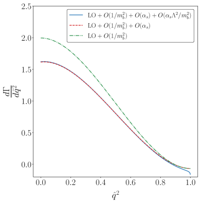
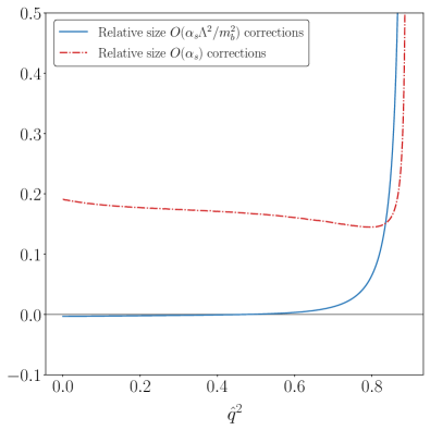
Figure 1: Left panel: $\hat{q}^{2}$ distribution in units $\Gamma_{0}$ at tree level (dashed-dotted line), including $O(\alpha_{s})$ corrections (dashed line) and including also $O(\alpha_{s}\Lambda^{2}/m_{b}^{2})$ corrections (solid line). Right panel: relative size of the $O(\alpha_{s})$ (dashed-dotted line) and $O(\alpha_{s}\Lambda^{2}/m_{b}^{2})$ (solid line) corrections.

The results for $W_{i}^{(\pi,1)}$ and $W_{i}^{(G,1)}$ in the massless case can be employed in Eq. (2) to compute the $O(\alpha_{s}\Lambda^{2}/m_{b}^{2})$ corrections to the total rate and to the moments of various differential distributions in $B\to X_{u}\ell\nu$. We first compute the total rate in the pole mass scheme and find

$$\Gamma(B\to X_{u}\ell\nu)=\Gamma_{0}\Big{[}\Big{(}1-2.41\frac{\alpha_{s}}{\pi}\Big{)}\Big{(}1-\frac{\mu_{\pi}^{2}}{2m_{b}^{2}}\Big{)}-\Big{(}\frac{3}{2}+4.98\frac{\alpha_{s}}{\pi}\Big{)}\frac{\mu_{G}^{2}(m_{b})}{m_{b}^{2}}\Big{]},$$ (6.1)

where $\Gamma_{0}=G_{F}^{2}|V_{ub}|^{2}m_{b}^{5}/192\pi^{3}$ is the lowest order result, and the $O(\alpha_{s})$ contributions are a standard result, see DeFazio:1999ptt . As already discussed, the $O(\alpha_{s}\mu_{\pi}^{2}/m_{b}^{2})$ corrections are dictated by RI. The non-trivial $O(\alpha_{s}\mu_{G}^{2}/m_{b}^{2})$ correction to the total width is sizeable and amounts to almost a quarter of the $O(\mu_{G}^{2}/m_{b}^{2})$ correction, but comes with a sign opposite to the $O(\alpha_{s}\mu_{\pi}^{2}/m_{b}^{2})$ correction and tends to cancel it. Using $\alpha_{s}=0.22$, $m_{b}=4.55$GeV, $\mu_{\pi}^{2}=0.43$GeV² and $\mu_{G}^{2}(m_{b})=0.35$GeV², the total shift induced by $O(\alpha_{s}\Lambda^{2}/m_{b}^{2})$ contributions amounts to -0.4%. Our result for the $O(\alpha_{s}\mu_{G}^{2}/m_{b}^{2})$ correction to the total width agrees with Ref. Mannel:2015jka , where the $O(\alpha_{s}\mu_{G}^{2}/m_{b}^{2})$ correction to the total width and to a few $q^{2}$ moments has been computed in an expansion in $m_{c}/m_{b}$, and the limit $m_{c}\to 0$ can be read from the first term in the expansion.

We have also computed the $\hat{q}^{2}$ distribution. It is displayed in Fig. 1, using the same inputs as above. One observes that the total correction is very small over the whole $\hat{q}^{2}$ range, except close to the endpoint, which is a region dominated by soft dynamics.

As explained in the Introduction, the rate subject to experimental cuts is determined by shape functions (SFs) that satisfy OPE constraints. Indeed, the corrections we have computed in this paper have an important effect on these constraints, which are related to the $\hat{q}_{0}$-moments of the form factors $W_{i}$. In the GGOU framework of Ref. Gambino:2007rp , a $q^{2}$-dependent SF is associated to each form factor $W_{i}$, which is in turn described by the convolution formula

$$W_{i}(\hat{q}_{0},\hat{q}^{2},\hat{\mu})=\int F_{i}(\kappa,\hat{q}^{2},\hat{\mu})W_{i}^{pert}\left[\hat{q}_{0}-\frac{\kappa}{2}\left(1-\frac{\hat{q}^{2}m_{b}}{m_{B}}\right),\hat{q}^{2},\hat{\mu}\right]d\kappa.$$ (6.2)

Here $W_{i}^{pert}$ represents the purely perturbative part of the structure functions in the kinetic scheme, and the structure function $W_{i}$ depends on a hard cutoff $\mu=\hat{\mu}m_{b}\sim 1$GeV that is meant to separate perturbative and non-perturbative contributions. While the SFs $F_{i}$ describe all nonperturbative physics, the $\hat{q}_{0}$-moments (or equivalently ${\hat{u}}$-moments) of (6.2) must match their OPE prediction, which can be shown to place constraints on the SFs moments, $\int\kappa^{n}F_{i}(\kappa,\hat{q}^{2},\hat{\mu})d\kappa$. This matching has been performed at the tree-level in Gambino:2007rp but the $O(\alpha_{s}\Lambda^{2}/m_{b}^{2})$ calculation of this paper permits to extend it at $O(\alpha_{s})$.

In the following we compute the first three $\hat{q}_{0}$-moments up to $O(\alpha_{s}\Lambda^{2}/m_{b}^{2})$ for fixed $\hat{q}^{2}$, leaving a detailed discussion of the constraints on the SFs to a future publication, which will also deal with the phenomenological consequences.

Let us consider the central moments of the power suppressed contributions

$$J_{i,X}^{(n,j)}(\hat{q}^{2}) =\int_{0}^{\infty}(\hat{q}_{0}-\hat{q}_{0}^{\,max})^{n}\,W_{i}^{(X,j)}(\hat{q}_{0},\hat{q}^{2})\,d\hat{q}_{0},$$ (6.3)

where $j=0,1$ and $X=\pi,G$. While the upper endpoint in the real radiation contributions is

$$\hat{q}_{0}^{\,max}=\frac{1+\hat{q}^{2}}{2},$$ (6.4)

and follows from the $\theta(\hat{u})$ in the expressions for $W_{i}^{(X,j)}$, the lower boundary for the integrals in Eq. (6.3) is an arbitrary choice, which coincides with the physical range of the semileptonic $B$ decay

$$\sqrt{\hat{q}^{2}}\leq\hat{q}_{0}\leq\frac{1+\hat{q}^{2}}{2}$$ (6.5)

only at $\hat{q}^{2}=0$. On the other hand, we note that the physical range (6.5) becomes narrower for larger $\hat{q}^{2}$ and vanishes at the maximal value, $\hat{q}^{2}=1$. In order to include in the integration most of the nonperturbative part of the spectral function, we therefore consider a larger range. This will be important for placing meaningful constraints on the SFs in the GGOU framework Gambino:2007rp , where there is a $q^{2}$-dependent SF associated to each form factor $W_{i}$, and the $J_{i,X}^{(n,i)}$ are the building blocks necessary to achieve that.

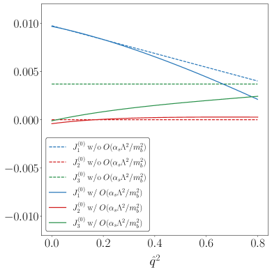
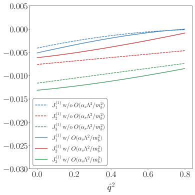
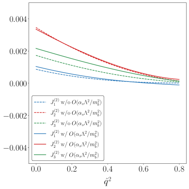
Figure 2: Power corrections to the lowest, first and second $\hat{q}_{0}$-moments of the form factors $W_{i}(\hat{q}_{0},\hat{q}^{2})$ on $\hat{q}^{2}$, with (solid lines) and without (dashed lines) the $O(\alpha_{s}\Lambda^{2}/m_{b}^{2})$ corrections.

The tree-level expressions $J_{i,X}^{(n,0)}(\hat{q}^{2})$ are given in the Appendix of Ref. Gambino:2007rp , while the $O(\alpha_{s})$ and $O(\alpha_{s}\Lambda^{2}/m_{b}^{2})$ corrections can be computed from the expressions for $W_{i}^{(1)}$ and $W_{i}^{(X,1)}$, respectively. In the Appendix we provide analytic results for $J_{i,\pi}^{(n,1)}(0)$ and $J_{i,G}^{(n,1)}(0)$. Let us also introduce

$$J_{i}^{(n)}(\hat{q}^{2}) =\dfrac{\mu_{\pi}^{2}}{2m_{b}^{2}}J_{i,\pi}^{(n,0)}(\hat{q}^{2})+\dfrac{\mu_{G}^{2}}{2m_{b}^{2}}J_{i,G}^{(n,0)}(\hat{q}^{2})+\dfrac{\alpha_{s}}{\pi}\left[\dfrac{\mu_{\pi}^{2}}{2m_{b}^{2}}C_{F}J_{i,\pi}^{(n,1)}(\hat{q}^{2})+\dfrac{\mu_{G}^{2}}{2m_{b}^{2}}J_{i,G}^{(n,1)}(\hat{q}^{2})\right].$$

In Fig. 2 we compare the moments $J_{i}^{(n)}$ with and without the $O(\alpha_{s}\Lambda^{2}/m_{b}^{2})$ corrections. We employ again the same inputs as before. The $O(\alpha_{s}\Lambda^{2}/m_{b}^{2})$ corrections to the zeroth moments are relatively small in most of the $\hat{q}^{2}$ range for $J_{1,2}^{(0)}$, and significant for $J_{3}^{(0)}$. We observed that if we compute the zeroth moments in the physical range (6.5), the impact of $O(\alpha_{s}\Lambda^{2}/m_{b}^{2})$ corrections is much larger, with the exception of the smallest values of $\hat{q}^{2}$. The reason why this does not imply large $O(\alpha_{s}\Lambda^{2}/m_{b}^{2})$ corrections to the total width and the $q^{2}$ spectrum has to do with the prefactors of $W_{i}$ in the differential width. For what concerns the higher moments, the $O(\alpha_{s}\Lambda^{2}/m_{b}^{2})$ corrections are generally moderate, but significant in a few cases, as a consequence of cancellations occurring at the tree level.

7 Summary

We have presented an analytic calculation of the $O(\alpha_{s})$ corrections to the Wilson coefficient of the kinetic and chromomagnetic operators in inclusive semileptonic decays without charm. Our results agree with reparametrization invariance relations and with a previous result on the total width. We find small corrections to the total rate and to the $q^{2}$ spectrum, generally below 1% and more significant corrections to some of the moments of the form factors. Our results place constraints on the SFs that describe $B\to X_{u}\ell\nu$ decays, and in particular allow for a determination of the perturbative corrections to their moments. This may prove useful in view of the higher precision expected at Belle II.

Appendix

In this Appendix we report the main results of our calculation. In particular, the perturbative corrections to the power corrections related to the kinetic operator are given by

$$W_{1}^{(\pi,1)} \!\!\!= \!\!w\Big{[}B_{1}-\frac{C}{2}+\frac{5w-2}{12}\Big{[}\frac{1}{\hat{u}^{2}}\Big{]}_{+}+\Big{(}\frac{16+3w-10w^{2}}{12}-\frac{8w^{3}-w^{2}-14w+8}{6(1-w)}\ln w\Big{)}\delta^{\prime}(\hat{u})\Big{]}$$ (A.1)

$$\!\!\!-\frac{4}{3}(2\!-\!w)\Big{(}\Big{[}\frac{\ln\hat{u}}{\hat{u}}\Big{]}_{+}\!\!+L_{w}\delta(\hat{u})\Big{)}+\Big{(}\frac{8}{3}(2\!-\!w)\ln w-\frac{4+\!18w\!-\!13w^{2}}{6w}\Big{)}\Big{[}\frac{1}{\hat{u}}\Big{]}_{+}\!\!+{\cal R}_{1}^{(\pi)}\theta(\hat{u})$$

$$\!\!\!+\Big{(}\frac{13w}{12}-\frac{1}{6}-\frac{1}{3w}-\frac{w^{2}}{12}+\frac{w^{3}}{4}+\frac{4+6w-13w^{2}+3w^{3}+2w^{5}}{3w(1-w)}\ln w\Big{)}\delta(\hat{u})$$

$$W_{2}^{(\pi,1)}\!\! = \!4B_{2}+6C+\frac{9w-10}{3}\Big{[}\frac{1}{\hat{u}^{2}}\Big{]}_{+}+\Big{(}\frac{4+6w+16w^{2}}{3}\ln w-\frac{22-21w+10w^{2}}{3}\Big{)}\delta^{\prime}(\hat{u})$$ (A.2)

$$\!\!\!+\Big{(}w^{2}+\frac{116}{3w^{2}}-7w-\frac{50}{w}+\frac{88}{3}-4\,\frac{42-34w+17w^{2}-6w^{3}+2w^{4}}{3w^{2}}\ln w\Big{)}\delta(\hat{u})$$

$$\!\!\!+\Big{(}\frac{10}{3}-\frac{68}{3w}+\frac{28}{w^{2}}\Big{)}\Big{[}\frac{1}{\hat{u}}\Big{]}_{+}+{\cal R}_{2}^{(\pi)}\theta(\hat{u})$$

$$W_{3}^{(\pi,1)} \!\!= \!\!2B_{3}+C+\Big{(}\frac{7w}{6}-1\Big{)}\Big{[}\frac{1}{\hat{u}^{2}}\Big{]}_{+}+\Big{(}\frac{5}{3}(1-w)w+\frac{w(6+3w-8w^{2})}{3(1-w)}\ln w\Big{)}\delta^{\prime}(\hat{u})$$ (A.3)

$$\!\!\!+2\Big{[}\frac{\ln\hat{u}}{\hat{u}}\Big{]}_{+}\!\!+\Big{(}\frac{19}{6}-\frac{2}{w}+\frac{4}{w^{2}}-4\ln w\Big{)}\Big{[}\frac{1}{\hat{u}}\Big{]}_{+}\!\!+\Big{[}2L_{w}+\frac{w^{2}}{2}+\frac{14}{3w^{2}}-\frac{11w}{6}-\frac{20}{3w}$$

$$\!\!\!+\frac{41}{6}+\Big{(}\frac{7w-6}{1-w}+\frac{4}{3}w-\frac{4}{3}w^{2}-\frac{8}{w^{2}}+\frac{4}{w}\Big{)}\ln w\Big{]}\delta(\hat{u})+{\cal R}_{3}^{(\pi)}\theta(\hat{u})$$

$$B_{i}=\frac{w^{2}}{6}\bigg{(}\Big{[}\frac{7}{4}-2L_{w}-\frac{2-w}{1-w}\ln w+\delta_{i2}\frac{\ln w}{1-w}\Big{]}\delta^{\prime\prime}(\hat{u})-4\Big{[}\frac{\ln\hat{u}}{\hat{u}^{3}}\Big{]}_{+}+(8\ln w-1)\Big{[}\frac{1}{\hat{u}^{3}}\Big{]}_{+}\bigg{)},$$

$$C=\frac{2(2-w)}{3}\bigg{(}-\Big{[}\frac{\ln\hat{u}}{\hat{u}^{2}}\Big{]}_{+}+2\ln w\Big{[}\frac{1}{\hat{u}^{2}}\Big{]}_{+}+L_{w}\,\delta^{\prime}(\hat{u})\bigg{)}$$ (A.4)

$$L_{w}={\rm Li}_{2}(1-w)+2\ln^{2}w+\frac{\pi^{2}}{3}$$

$${\cal R}_{1}^{(\pi)} \!\!\!= \!\!\frac{(4\hat{u}-w)(2-w)\hat{u}+2w^{3}}{3\hat{u}^{3}}\ln\frac{\hat{u}}{w^{2}}+\Big{[}\frac{2w^{6}}{3\hat{u}^{3}}+\frac{7w^{5}}{3\hat{u}^{2}}-\frac{14-5\hat{u}}{3\hat{u}^{2}}w^{4}-\frac{13\hat{u}+32}{6\hat{u}}w^{3}$$

$$-\frac{23\hat{u}^{2}-36\hat{u}-48}{6\hat{u}}w^{2}-(13\hat{u}^{2}-58\hat{u}+36)\frac{w}{6}-\frac{\hat{u}}{6}(3\hat{u}^{2}-26\hat{u}+8)\Big{]}\frac{{\cal I}_{1}}{\tilde{\lambda}}$$

$$-\frac{4w^{2}}{3\hat{u}^{2}}+\frac{2\hat{u}^{2}+2\hat{u}w-13\hat{u}+17w-28}{3\tilde{\lambda}}+\frac{4w}{3\hat{u}^{2}}+\frac{2}{3\hat{u}w}-\frac{7\hat{u}+8}{12\hat{u}}$$

$${\cal R}_{2}^{(\pi)}\!\! \!= \!\!\frac{12(2\!-\!w)\hat{u}+8w^{2}}{3\hat{u}^{3}}\ln\frac{\hat{u}}{w^{2}}+\bigg{[}w\Big{(}\frac{8w^{4}}{3\hat{u}^{3}}-\!\frac{40}{3}-\!\frac{14w}{3}\!-\!2\hat{u}+\frac{(4w\!-\!8)w^{2}}{\hat{u}^{2}}-4\frac{8-8w+w^{2}}{\hat{u}}\Big{)}$$

$$+68+\!60\hat{u}-\!\frac{4}{\tilde{\lambda}}\big{(}15\hat{u}^{3}-35\hat{u}^{2}-76\hat{u}+14w+63w\hat{u}+19w\hat{u}^{2}\big{)}\bigg{]}\frac{{\cal I}_{1}}{\tilde{\lambda}}+\frac{16(1+2\hat{u})}{3\hat{u}^{2}}$$

$$-\frac{16w}{3\hat{u}^{2}}-\frac{28}{\hat{u}w^{2}}+\frac{68}{3\hat{u}w}-\frac{2\left(9\hat{u}^{2}+50\hat{u}w-201\hat{u}+86w-78\right)}{3\hat{u}\tilde{\lambda}}$$

$$-\frac{4\left(2\hat{u}^{2}w+2\hat{u}^{3}+11\hat{u}^{2}+49\hat{u}w-81\hat{u}+45w-28\right)}{\tilde{\lambda}^{2}}$$

$${\cal R}_{3}^{(\pi)} \!\!\!= \!-\frac{2(3\hat{u}^{2}-(2-w)\hat{u}-2w^{2})}{3\hat{u}^{3}}\ln\frac{\hat{u}}{w^{2}}+\Big{(}8w-\frac{13}{3}w^{2}-4-\frac{10}{3}\hat{u}(w-2)-\hat{u}^{2}$$

$$+\frac{10\hat{u}(w-2)w^{3}+4w^{5}}{3\hat{u}^{3}}\Big{)}\frac{{\cal I}_{1}}{\tilde{\lambda}}-\frac{2\left(7\hat{u}^{2}+11\hat{u}w-19\hat{u}+17w-16\right)}{3\hat{u}\tilde{\lambda}}$$

$$-\frac{8w}{3\hat{u}^{2}}+\frac{8(\hat{u}+1)}{3\hat{u}^{2}}-\frac{4}{\hat{u}w^{2}}+\frac{2}{\hat{u}w}$$

In the above expressions the coefficients of the derivatives of $\delta(\hat{u})$ have been reduced using integration by parts identities like

$$f(\hat{u})\,\delta^{\prime\prime}(\hat{u})=f(0)\,\delta^{\prime\prime}(\hat{u})-2f^{\prime}(0)\,\delta^{\prime}(\hat{u})+f^{\prime\prime}(0)\,\delta(\hat{u}),$$ (A.8)

as well as identities such as (4.4) and (4.22).

The analogous results for the coefficients of the matrix element of the chromomagnetic operator are

$$W_{1}^{(G,1)} \!\!\!= \!\!-\frac{2}{3}w\bigg{[}G_{1}+\Big{(}\mbox{\small$\frac{C_{F}}{4}$}\Big{(}1+8w-5\frac{w^{2}\ln w}{1-w}\Big{)}-\mbox{\small$\frac{C_{A}}{4}$}(1+2w)\Big{)}\delta^{\prime}(\hat{u})$$

$$\!\!+\mbox{\small$C_{F}(5+\frac{2}{w^{2}}-\frac{2}{w})$}\Big{(}\Big{[}\frac{\ln\hat{u}}{\hat{u}}\Big{]}_{+}\!\!-\!2\ln w\Big{[}\frac{1}{\hat{u}}\Big{]}_{+}\!\!+\!L_{w}\delta(\hat{u})\Big{)}\Big{]}$$

$$\!\!-\frac{2}{3}\Big{(}\mbox{\small$\frac{C_{A}}{4}$}(8\!-\!5w)+C_{F}\big{(}\frac{4}{w}-3+\frac{5w}{4}\big{)}\Big{)}\Big{[}\frac{1}{\hat{u}}\Big{]}_{+}$$

$$\!\!-\frac{1}{3}\big{(}\mbox{\small$C_{A}\frac{5w^{3}-34w^{2}+51w-20}{2(w-1)^{2}}+C_{F}\frac{10w^{5}-21w^{4}+7w^{3}-10w^{2}+28w-16}{(w-1)^{2}w}$}\big{)}\ln w\,\delta(\hat{u})$$

$$\!\!-\frac{1}{3}\big{(}\mbox{\small$C_{A}\frac{2w^{4}+2w^{3}-3w^{2}+5w-4}{2(1-w)w}+C_{F}\frac{35w^{3}-25w^{2}-10w-8}{4(1-w)}$}\big{)}\delta(\hat{u})+{\cal R}_{1}^{(G)}\theta(\hat{u})$$

$$W_{2}^{(G,1)} \!\!= \!\!-\frac{8}{3}\Big{[}G_{2}+\Big{(}\mbox{\small$C_{F}$}\Big{(}\frac{1}{w}-\frac{11}{4}+2w-(1-\frac{5w}{4})\ln w\Big{)}+\mbox{\small$\frac{C_{A}}{4}$}(3-2w)\Big{)}\delta^{\prime}(\hat{u})$$

$$\!\!\!\!+\mbox{\small$2C_{F}\frac{w^{2}-w-1}{w^{3}}$}\Big{(}\Big{[}\frac{\ln\hat{u}}{\hat{u}}\Big{]}_{+}\!\!-\!2\ln w\Big{[}\frac{1}{\hat{u}}\Big{]}_{+}\!\!+\!L_{w}\delta(\hat{u})\Big{)}$$

$$\!\!\!\!+\!\big{(}\mbox{\small$C_{A}(\frac{8}{w}-\frac{9}{2w^{2}}-\frac{2}{w^{3}}-\frac{9}{4})$}+\mbox{\small$C_{F}(\frac{7}{w^{2}}-\frac{6}{w^{3}}-\frac{5}{2})$}\big{)}\Big{[}\frac{1}{\hat{u}}\Big{]}_{+}$$

$$\!\!\!\!+\big{(}\mbox{\small$C_{A}\frac{9w^{3}-56w^{2}+40w+16}{4w^{3}}+C_{F}\frac{5w^{4}-6w^{3}+3w^{2}-12w+12}{w^{3}}$}\big{)}\ln w\,\delta(\hat{u})$$

$$\!\!\!\!-\big{(}\mbox{\small$C_{A}\frac{2w^{3}+4w^{2}-23w+16}{4w^{2}}+C_{F}\frac{35w^{4}-98w^{3}+134w^{2}-120w+32}{8w^{3}}$}\big{)}\delta(\hat{u})\Big{]}+{\cal R}_{2}^{(G)}\theta(\hat{u})$$

$$W_{3}^{(G,1)} \!\!\!\!= \!\!-\frac{4}{3}\Big{[}G_{3}+\Big{(}\mbox{\small$C_{F}$}\Big{(}\frac{1}{4}+\frac{5w}{2}-\frac{5w^{2}\ln w}{4(1-w)}\Big{)}-\mbox{\small$\frac{C_{A}}{4}$}(1+w)\Big{)}\delta^{\prime}(\hat{u})\Big{]}$$

$$\!\!-\frac{2}{3}\mbox{\small$C_{F}\frac{5w^{2}+4w+4}{w^{2}}$}\Big{(}\Big{[}\frac{\ln\hat{u}}{\hat{u}}\Big{]}_{+}\!\!-\!2\ln w\Big{[}\frac{1}{\hat{u}}\Big{]}_{+}\!+L_{w}\delta(\hat{u})\Big{)}$$

$$\!\!-\frac{2}{3}\big{(}\mbox{\small$C_{A}(\frac{2}{w^{2}}+\frac{5}{w}-\frac{7}{2})$}+\mbox{\small$C_{F}(\frac{4}{w^{2}}-\frac{5}{4})$}\big{)}\Big{[}\frac{1}{\hat{u}}\Big{]}_{+}$$

$$\!\!-\frac{1}{3}\big{(}\mbox{\small$C_{A}\frac{7w^{4}-40w^{3}+49w^{2}-6w-8}{(w-1)^{2}w^{2}}+C_{F}\frac{(20w^{5}-37w^{4}-w^{3}+6w^{2}+24w-16)}{(w-1)^{2}w^{2}}$}\big{)}\ln w\,\delta(\hat{u})$$

$$\!\!-\frac{2}{3}\big{(}\mbox{\small$C_{A}\frac{w^{2}-w+1}{1-w}+C_{F}\frac{35w^{4}-85w^{3}+66w^{2}-8w-16}{4(1-w)w^{2}}$}\big{)}\delta(\hat{u})+{\cal R}_{3}^{(G)}\theta(\hat{u})$$

$$G_{i} = \!\!\Big{(}1+\frac{5}{2}w-4\delta_{i2}\Big{)}\bigg{[}\mbox{\small$C_{F}$}\Big{(}\frac{3-8\ln w}{4}\Big{[}\frac{1}{\hat{u}^{2}}\Big{]}_{+}+\Big{[}\frac{\ln\hat{u}}{\hat{u}^{2}}\Big{]}_{+}-L_{w}\delta^{\prime}(\hat{u})\Big{)}+\mbox{\normalsize$\frac{C_{A}}{2}$}\ln\frac{\mu}{m_{b}}\delta^{\prime}(\hat{u})\bigg{]}$$ (A.12)

$$\!\!\!\!+C_{A}\bigg{[}\frac{1\!+\!w}{2}\Big{[}\Big{[}\frac{1}{\hat{u}^{2}}\Big{]}_{+}\!\!+\ln w\,\delta^{\prime}(\hat{u})\Big{]}\!-\!\delta_{i2}\Big{(}\frac{1\!+\!2w}{2w}\Big{[}\frac{1}{\hat{u}^{2}}\Big{]}_{+}\!\!+\!\frac{\ln w}{w}\delta^{\prime}(\hat{u})\Big{)}\bigg{]}\!-\!\mbox{\normalsize$\frac{3C_{A}}{4}$}\frac{w_{i}^{(G,0)}}{w_{i}^{(0)}}\ln\frac{\mu}{m_{b}}\delta(\hat{u})$$

$$\!\!\!\!+C_{A}\Big{(}\frac{1+4w}{2w^{2}}-\frac{1+2w}{w^{3}}\delta_{i2}\Big{)}\bigg{[}\Big{[}\frac{\ln\hat{u}}{\hat{u}}\Big{]}_{+}-2\ln w\Big{[}\frac{1}{\hat{u}}\Big{]}_{+}+L_{w}\delta(\hat{u})\bigg{]}$$

where

$$w_{1}^{(G,0)}=-\frac{2}{3}(4-5w),\qquad w_{2}^{(G,0)}=0,\qquad w_{3}^{(G,0)}=\frac{10}{3},$$ (A.13)

and

$${\cal R}_{1}^{(G)}\!\! = \!\!\frac{C_{A}}{3}\Big{[}\mbox{$\frac{1}{2}+\frac{\hat{u}+13w-16}{\tilde{\lambda}}+\frac{4w+1}{\hat{u}w}\ln\frac{\hat{u}}{w^{2}}$}+\Big{(}\mbox{$\frac{4w+1-6\hat{u}}{\hat{u}}+2\frac{3\hat{u}(\hat{u}-3+w)+4w}{\tilde{\lambda}}$}\Big{)}{\cal I}_{1}\Big{]}$$

$$\!\!\!+\frac{C_{F}}{3}\Big{[}\mbox{$\frac{15\hat{u}-5\hat{u}w-5\hat{u}^{2}-11w+20}{\tilde{\lambda}}-\frac{4w}{\hat{u}\tilde{\lambda}}-\frac{10w}{\hat{u}}+\frac{8}{\hat{u}w}+\frac{11\hat{u}+24}{4\hat{u}}$}+\Big{(}\mbox{$\frac{5w^{2}}{\hat{u}^{2}}+\frac{2(5\hat{u}+1)w}{\hat{u}^{2}}+\frac{4-4w}{\hat{u}w}$}\Big{)}\ln\frac{\hat{u}}{w^{2}}$$

$$\!\!\!+\Big{(}\mbox{$\frac{8-3\hat{u}^{2}-13\hat{u}w+10\hat{u}-12w}{\tilde{\lambda}}+\frac{5w^{3}}{\hat{u}^{2}}+\frac{(15\hat{u}+2)w^{2}}{\hat{u}^{2}}+\frac{3(5\hat{u}-8)w}{2\hat{u}}+\frac{5\hat{u}}{2}-2$}\Big{)}{\cal I}_{1}\Big{]}$$

$${\cal R}_{2}^{(G)} \!\!\!= \!4C_{A}\Big{[}\mbox{$\frac{16-13\hat{u}^{2}-25\hat{u}w+51\hat{u}-29w}{\tilde{\lambda}^{2}}+\frac{22-15\hat{u}w-9\hat{u}^{2}+112\hat{u}-32w}{6\tilde{\lambda}\hat{u}}+\frac{w}{3\tilde{\lambda}\hat{u}^{2}}+\frac{16\hat{u}-1}{3\hat{u}^{2}w}-\frac{3}{\hat{u}w^{2}}-\frac{4}{3\hat{u}w^{3}}$}$$

$$\!\!\!+\mbox{$\frac{4w^{2}-3w-2}{3w^{3}\hat{u}}$}\ln\frac{\hat{u}}{w^{2}}+\Big{(}\mbox{$\frac{14\hat{u}^{2}-26\hat{u}w+58\hat{u}-3w-2}{3\tilde{\lambda}\hat{u}}-\frac{2\left(3\hat{u}^{2}w+3\hat{u}^{3}-5\hat{u}^{2}+20\hat{u}w-25\hat{u}\right)}{\tilde{\lambda}^{2}}-\frac{8w}{\tilde{\lambda}^{2}}+\frac{4}{3\hat{u}}$}\Big{)}{\cal I}_{1}\Big{]}$$

$$\!\!\!+4C_{F}\Big{[}\mbox{$\frac{5\hat{u}^{2}w+42\hat{u}w+5\hat{u}^{3}-4\hat{u}^{2}-55\hat{u}+39w-36}{\tilde{\lambda}^{2}}+\frac{4w}{\tilde{\lambda}^{2}\hat{u}}+\frac{53\hat{u}w-20\hat{u}^{2}-155\hat{u}+44w-52}{6\tilde{\lambda}\hat{u}}+\!\frac{14}{3\hat{u}w^{2}}\!-\!\frac{4}{\hat{u}w^{3}}\!-\!\frac{10}{3\hat{u}}$}$$

$$\!\!\!+\mbox{$\frac{4\hat{u}\left(w^{2}-w-1\right)+(5w-6)w^{3}}{3\hat{u}^{2}w^{3}}$}\ln\frac{\hat{u}}{w^{2}}+\Big{(}\mbox{$\frac{23\hat{u}^{2}w+13\hat{u}^{3}-37\hat{u}^{2}+47\hat{u}w-58\hat{u}+20w-8}{\tilde{\lambda}^{2}}$}$$

$$\!\!\!+\mbox{$\frac{25\hat{u}^{2}w+15\hat{u}^{3}-114\hat{u}^{2}+76\hat{u}w-150\hat{u}+16w-8}{6\tilde{\lambda}\hat{u}}+\frac{5w^{2}}{3\hat{u}^{2}}+\frac{(5\hat{u}-6)w}{3\hat{u}^{2}}-\frac{5\hat{u}+8}{2\hat{u}}$}\Big{)}{\cal I}_{1}\Big{]}$$

$${\cal R}_{3}^{(G)} \!\!\!=\!\!\! \frac{4C_{A}}{3}\Big{[}\mbox{$\frac{15\hat{u}-3\hat{u}^{2}-3\hat{u}w-5w-2}{2\tilde{\lambda}\hat{u}}+\frac{1}{\hat{u}w^{2}}+\frac{5}{2\hat{u}w}+\frac{1+4w}{2w^{2}\hat{u}}\ln\frac{\hat{u}}{w^{2}}+\frac{w-5\hat{u}-2w\hat{u}+4w^{2}}{2\tilde{\lambda}\hat{u}}$}{\cal I}_{1}\Big{]}\quad\qquad\qquad$$

$$+\frac{4C_{F}}{3}\Big{[}\mbox{$\frac{2\hat{u}^{2}+7\hat{u}w-9\hat{u}+3w}{\tilde{\lambda}\hat{u}}+\frac{2}{\hat{u}w^{2}}-\frac{5}{\hat{u}}+\Big{(}\frac{5w}{2\hat{u}^{2}}+\frac{5\hat{u}+2}{2\hat{u}^{2}}+\frac{2}{\hat{u}w^{2}}+\frac{2}{\hat{u}w}\Big{)}\ln\frac{\hat{u}}{w^{2}}$}$$

$$+\Big{(}\mbox{$\frac{5\hat{u}^{2}+5\hat{u}w-16\hat{u}+12w-12}{2\tilde{\lambda}}+\frac{5w^{2}}{2\hat{u}^{2}}+\frac{(5\hat{u}+1)w}{\hat{u}^{2}}-\frac{5\hat{u}+8}{4\hat{u}}$}\Big{)}{\cal I}_{1}\Big{]}$$

The $\hat{q}_{0}$-moments of the form factors are defined in Eq. (6.3). We first recall the tree-level results

$$J_{1}^{(0)}=\frac{1-\hat{q}^{2}}{2}+\frac{1+\hat{q}^{2}}{3}\frac{\mu_{\pi}^{2}}{m_{b}^{2}}+\frac{1-5\hat{q}^{2}}{6}\frac{\mu_{G}^{2}}{m_{b}^{2}},\qquad J_{2}^{(0)}=2,\qquad J_{3}^{(0)}=1-\frac{\mu_{\pi}^{2}}{2m_{b}^{2}}+\frac{5}{6}\frac{\mu_{G}^{2}}{m_{b}^{2}},$$

$$J_{1}^{(1)}=\frac{1-\hat{q}^{4}}{24}\frac{\mu_{\pi}^{2}}{m_{b}^{2}}-\frac{7-12\hat{q}^{2}+5\hat{q}^{4}}{24}\frac{\mu_{G}^{2}}{m_{b}^{2}},\qquad J_{2}^{(1)}=-\frac{1+\hat{q}^{2}}{2}\frac{\mu_{\pi}^{2}}{m_{b}^{2}}+\frac{1+5\hat{q}^{2}}{6}\frac{\mu_{G}^{2}}{m_{b}^{2}},$$

$$J_{3}^{(1)}=-\frac{1+\hat{q}^{2}}{12}\frac{\mu_{\pi}^{2}}{m_{b}^{2}}+\frac{5\hat{q}^{2}-7}{12}\frac{\mu_{G}^{2}}{m_{b}^{2}},\qquad J_{1}^{(2)}=\frac{(1-\hat{q}^{2})^{3}}{24}\frac{\mu_{\pi}^{2}}{m_{b}^{2}},$$

$$J_{2}^{(2)}=\frac{(1-\hat{q}^{2})^{2}}{6}\frac{\mu_{\pi}^{2}}{m_{b}^{2}},\qquad J_{3}^{(2)}=\frac{(1-\hat{q}^{2})^{2}}{12}\frac{\mu_{\pi}^{2}}{m_{b}^{2}}.$$ (A.17)

Finally, here we report the results of the $O(\alpha_{s}\Lambda^{2}/m_{b}^{2})$ corrections at $q^{2}=0$ with $\mu=m_{b}$:

$$J_{1,\pi}^{(0,1)}(0)=-\frac{\pi^{2}}{18},\qquad J_{1,\pi}^{(1,1)}(0)=\frac{151}{48}-\frac{25\pi^{2}}{72},\qquad J_{1,\pi}^{(2,1)}(0)=-\frac{191}{48}+\frac{7\pi^{2}}{18},$$

$$J_{2,\pi}^{(0,1)}(0)=0,\qquad J_{2,\pi}^{(1,1)}(0)=-\frac{5}{4}+\frac{\pi^{2}}{4},\qquad J_{2,\pi}^{(2,1)}(0)=\frac{35}{12}-\frac{11\pi^{2}}{36},$$ (A.18)

$$J_{3,\pi}^{(0,1)}(0)=-\frac{3}{4}+\frac{\pi^{2}}{12},\qquad J_{3,\pi}^{(1,1)}(0)=\frac{3}{8}+\frac{\pi^{2}}{72},\qquad J_{3,\pi}^{(2,1)}(0)=-\frac{11}{16}+\frac{7\pi^{2}}{144},$$

$$J_{1,G}^{(0,1)}(0)=\frac{121}{18}-\frac{65\pi^{2}}{108},\qquad J_{1,G}^{(1,1)}(0)=-\frac{11}{16}-\frac{13\pi^{2}}{216},\qquad J_{1,G}^{(2,1)}(0)=\frac{707}{2592}+\frac{11\pi^{2}}{432},$$

$$J_{2,G}^{(0,1)}(0)=-\frac{59}{6}+\frac{25\pi^{2}}{27},\quad J_{2,G}^{(1,1)}(0)=\frac{109}{36}-\frac{7\pi^{2}}{27},\quad J_{2,G}^{(2,1)}(0)=-\frac{317}{72}+\frac{4\pi^{2}}{9},$$ (A.19)

$$J_{3,G}^{(0,1)}(0)=\frac{28}{3}-\frac{29\pi^{2}}{18},\qquad J_{3,G}^{(1,1)}(0)=-\frac{29}{9}-\frac{\pi^{2}}{54},\qquad J_{3,G}^{(2,1)}(0)=\frac{371}{144}-\frac{11\pi^{2}}{72},$$

References

- (1) M. Neubert, Phys. Rev. D 49 (1994), 3392-3398 [arXiv:hep-ph/9311325 [hep-ph]].
- (2) I. I. Y. Bigi, M. A. Shifman, N. G. Uraltsev and A. I. Vainshtein, Int. J. Mod. Phys. A 9 (1994), 2467-2504 [arXiv:hep-ph/9312359 [hep-ph]].
- (3) B. O. Lange, M. Neubert and G. Paz, Phys. Rev. D 72 (2005), 073006 [arXiv:hep-ph/0504071 [hep-ph]].
- (4) P. Gambino, P. Giordano, G. Ossola and N. Uraltsev, JHEP 10 (2007), 058 [arXiv:0707.2493 [hep-ph]].
- (5) J. R. Andersen and E. Gardi, JHEP 01 (2006), 097 [arXiv:hep-ph/0509360 [hep-ph]].
- (6) Y. S. Amhis et al. [HFLAV], [arXiv:1909.12524 [hep-ex]].
- (7) J. P. Lees et al. [BaBar], Phys. Rev. D 95 (2017) no.7, 072001 [arXiv:1611.05624 [hep-ex]].
- (8) L. Cao et al. [Belle], [arXiv:2102.00020 [hep-ex]].
- (9) P. Gambino, A. S. Kronfeld, M. Rotondo, C. Schwanda, F. Bernlochner, A. Bharucha, C. Bozzi, M. Calvi, L. Cao and G. Ciezarek, et al. Eur. Phys. J. C 80 (2020) no.10, 966 [arXiv:2006.07287 [hep-ph]].
- (10) Z. Ligeti, I. W. Stewart and F. J. Tackmann, Phys. Rev. D 78 (2008), 114014 [arXiv:0807.1926 [hep-ph]].
- (11) F. U. Bernlochner et al. [SIMBA], arXiv:2007.04320 [hep-ph].
- (12) P. Gambino, K. J. Healey and C. Mondino, Phys. Rev. D 94 (2016) no.1, 014031 [arXiv:1604.07598 [hep-ph]].
- (13) M. Brucherseifer, F. Caola and K. Melnikov, Phys. Lett. B 721 (2013), 107-110 doi:10.1016/j.physletb.2013.03.006 [arXiv:1302.0444 [hep-ph]].
- (14) A. Alberti, T. Ewerth, P. Gambino and S. Nandi, Nucl. Phys. B 870 (2013), 16-29 [arXiv:1212.5082 [hep-ph]].
- (15) A. Alberti, P. Gambino and S. Nandi, JHEP 01 (2014), 147 [arXiv:1311.7381 [hep-ph]].
- (16) T. Becher, H. Boos and E. Lunghi, JHEP 0712 (2007) 062 [arXiv:0708.0855].
- (17) T. Mannel, A. A. Pivovarov and D. Rosenthal, Phys. Rev. D 92 (2015) no.5, 054025 [arXiv:1506.08167 [hep-ph]].
- (18) A. V. Manohar, Phys. Rev. D 82 (2010) 014009 [arXiv:1005.1952 [hep-ph]].
- (19) I. I. Y. Bigi, N. G. Uraltsev and A. I. Vainshtein, Phys. Lett. B 293 (1992) 430 [Erratum-ibid. B 297 (1993) 477] [arXiv:hep-ph/9207214]; I. I. Y. Bigi, M. A. Shifman, N. G. Uraltsev and A. I. Vainshtein, Phys. Rev. Lett. 71 (1993) 496 [arXiv:hep-ph/9304225].
- (20) B. Blok, L. Koyrakh, M. A. Shifman and A. I. Vainshtein, Phys. Rev. D 49 (1994) 3356 [Erratum-ibid. D 50 (1994) 3572] [arXiv:hep-ph/9307247]; A. V. Manohar and M. B. Wise, Phys. Rev. D 49 (1994) 1310 [arXiv:hep-ph/9308246].
- (21) V. Aquila, P. Gambino, G. Ridolfi and N. Uraltsev, Nucl. Phys. B 719 (2005) 77 [arXiv:hep-ph/0503083].
- (22) F. De Fazio and M. Neubert, JHEP 06 (1999), 017 [arXiv:hep-ph/9905351 [hep-ph]].
- (23) M. E. Luke and A. V. Manohar, Phys. Lett. B 286 (1992) 348 [hep-ph/9205228].
- (24) A. V. Manohar and M. B. Wise, Camb. Monogr. Part. Phys. Nucl. Phys. Cosmol. 10 (2000) 1.
- (25) M. Fael, T. Mannel and K. Keri Vos, JHEP 02 (2019), 177 [arXiv:1812.07472 [hep-ph]].