VVV survey near-infrared colour catalogue of known variable stars

Abstract

Context. The Vista Variables in the Via Lactea (VVV) near-infrared variability survey explores some of the most complex regions of the Milky Way bulge and disk in terms of high extinction and high crowding.

Aims. We add a new wavelength dimension to the optical information available at the American Association of Variable Star Observers International Variable Star Index (VSX-AAVSO) catalogue to test the VVV survey near-infrared photometry to better characterise these objects.

Methods. We cross-matched the VVV and the VSX-AAVSO catalogues along with Gaia Data Release 2 photometry and parallax.

Results. We present a catalogue that includes accurate individual coordinates, near-infrared magnitudes ($ZYJHK{\rm s}$), extinctions $A_{Ks}$, and distances based on Gaia parallaxes. We also show the near-infrared CMDs and spatial distributions for the different VSX types of variable stars, including important distance indicators, such as RR Lyrae, Cepheids, and Miras. By analysing the photometric flags in our catalogue, we found that about 20% of the stars with measured and verified variability are flagged as non-stellar sources, even when they are outside of the saturation and/or noise regimes. Additionally, we pair-matched our sample with the VIVA catalogue and found that more than half of our sources are missing from the VVV variability list, mostly due to observations with low signal-to-noise ratio or photometric problems with a low percentage due to failures in the selection process.

Conclusions. Our results suggest that the current knowledge of the variability in the Galaxy is biased to nearby stars with low extinction. The present catalogue also provides the groundwork for characterising the results of future large variability surveys such as the Vera C. Rubin Observatory Legacy Survey of Space and Time in the highly crowded and reddened regions of the Galactic plane, as well as follow-up campaigns for characterising specific types of variables. The analysis of the incorrectly flagged stars can be used to improve the photometric classification of the VVV data, allowing us to expand the amount of data considered useful for science purposes. In addition, we provide a list of stars that are missed by the VIVA procedures for which the observations are good and which were missed due to some failure in the VIVA selection process.

1 Introduction

The variable stars in the Milky Way are almost countless. Since the discovery of the first of these objects, the number of variable stars has increased consistently. Pigott & Englefield (1786) provided one of the first catalogues of stellar variability, containing a total of 12 objects known as being variable at that time. Many other catalogues have been released since then, especially within the past two decades, when large digital survey telescopes became operational, scanning the sky night after night, such as the Infrared Astronomical Satellite (IRAS, Neugebauer et al., 1984), the Two Micron All-Sky Survey (2MASS, Kleinmann et al., 1994), the Sloan Digital Sky Survey (SDSS, York et al., 2000), the Catalina Sky Surveys (Drake et al., 2014, 2017), the Panoramic Survey Telescope and Rapid Response System (Pan-STARRS, Kaiser et al., 2002), the UKIRT Infrared Deep Sky Survey (UKIDSS, Lawrence et al., 2007), the AKARI Far-infrared All-Sky Survey (AKARI, Ishihara et al., 2010), the Wide-field Infrared Survey Explorer (WISE, Wright et al., 2010; Chen et al., 2018a, b), and the Gaia spectroscopic survey (Gaia, Gilmore et al., 2012; Gaia Collaboration et al., 2016), as well the ongoing All-Sky Automated Survey for Supernovae (ASAS-SN; Jayasinghe et al., 2018). In addition, the large microlensing surveys, such as the Massive Astrophysical Compact Halo Objects (MACHO; Alcock et al., 1993), the Optical Gravitational Lensing Experiment (OGLE; Udalski et al., 1993), the Experience pour la Recherche d’Objets Sombres (EROS; Aubourg et al., 1993), the Microlensing Observations in Astrophysics (MOA; Bond et al., 2001), the Disk Unseen Objects (DUO; Alard et al., 1995), and the Korea Microlensing Telescope Network (KMTNet; Kim et al., 2016), have discovered hundreds of thousands of variable stars in the past decades.

These projects provide a new view of the variability in the Galaxy, and this subject is expected to become yet more interesting. The future of this field of study in the Milky Way will be revolutionised by the Vera C. Rubin Observatory Legacy Survey of Space and Time (LSST, Ivezic et al. 2008), which is expected to discover millions of variables. Another important aspect to consider is the contrast between near-infrared and optical variability. The searches performed at different wavelengths result in different relative numbers, and this must be considered when the number of variable stars that will be present in the LSST catalogues is predicted (e.g. Pietrukowicz et al., 2012).

However, most of the current projects searching for variables operate with optical telescopes, thus avoiding the innermost Milk Way plane, where high extinction and crowding limit the depth at optical wavelengths. Therefore an infrared survey is more suitable for the mission of observing deeper into the Galaxy plane, as does the VISTA Variables in The Vía Láctea (VVV), which is an European Southern Observatory (ESO) public survey that mapped the bulge ($-10.0^{\circ}\lesssim l\lesssim+10.5^{\circ}$ and $-10.3^{\circ}\lesssim b\lesssim+5.1^{\circ}$) and the inner southern part of the disk ($294.7^{\circ}\lesssim l\lesssim+350.0^{\circ}$ and $-2.25^{\circ}\lesssim b\lesssim+2.25^{\circ}$) of our Galaxy using five near-infrared bands ($Z$, $Y$, $J$, $H$ and $K_{\rm s}$; Minniti et al., 2010) plus a variability campaign in $K_{\rm s}$ band with typically 100 epochs per field in the period 2010-2017. The VVV Survey was completed in 2017 when its extension, the VVV eXtended Survey (Minniti, 2018), started observing to increase the observed area of VVV from 562 to 1700 sq. deg., filling the gaps between the VVV and the VISTA Hemisphere Survey (VHS McMahon et al., 2013).

Near-infrared surveys such as the VVV are very efficient at low Galactic latitudes close to the plane, where existing optical variability surveys are usually blinded by the absorption in the interstellar medium. For instance, VVV data were used to find RR Lyrae stars within 100 arcmin from the Galactic Centre (Contreras Ramos et al., 2018). In the same way that Baade’s Window was important for optical studies of the Galactic bulge, the near-infrared surveys also profit from the study of the windows that have recently been found in the Milky Way plane (e.g. Dante’s Window; Minniti et al., 2018).

Focusing on the subject of variables stars, the International Variable Star Index (VSX), provided by the American Association of Variable Star Observers (AAVSO), compiles a large number of known variable objects into a single database containing 1 432 563 objects as of February 1, 2020. This work compiles information from various catalogues such as those mentioned before, together with a brief analysis of missed sources in one of the more complete variability catalogues for the galactic bulge existing to date, the VISTA Variables in the Vía Láctea infrared variability catalogue (VIVA, Ferreira Lopes et al., 2020).

Here we present a catalogue with near-infrared colours for the VSX sources based on VVV data. This work provides useful information such as the colours in the $ZYJHK_{\rm s}$ bands, the extinction in the near-infrared ($A_{K\mathrm{s}}$), and the distances based on the parallaxes of Gaia Data Release 2 (Gaia DR2; Gaia Collaboration et al., 2018, 2019). Near-infrared colour-magnitude diagrams (CMDs) and the surface density distribution for the different types of variable stars include important distance indicators such as RR Lyrae, Cepheids and Miras. Section 2 presents the data we used and some statistics of our sample, in Section 3 we classify the variable stars in our catalogue in context with distance and period ($P$), in Section 4 we discuss the sources that were missed in the construction of the VIVA catalogue, and in Section 5 we summarise our results.

2 Data

Many catalogues of variable stars are available electronically, such as the General Catalogue of Variable Stars (GCVS, Samus’ et al. 2017), the All-Sky Automated Survey (ASAS, Pojmanski et al. 2005), and the Catalog and Atlas of Cataclysmic Variables (Downes et al., 2001). As part of this sample of catalogues, objects are discovered by important variability surveys of the inner Milky Way such as OGLE (e.g. Udalski et al., 2015), MOA (Alcock et al., 1997) , and even VVV. The VSX catalogue contains names, positions, period, the VSX type, and astronomical information, such as the constellation they belong to, and the passband that was used to measure the variability, which is mostly observed in the optical.

2.1 Cross-matching the VVV data with the VSX catalogue

While the VSX catalogue contains data for the whole sky, the VVV survey covered a total of 562 sq. deg., which is about 1.4 $\%$ of the celestial sphere. Although it covers only a small fraction of the sky, the VVV concentrated its observations on the most crowded regions of the southern sky, which are the Milk Way bulge and southern plane. The projected cone of view covers $\sim$30 $\%$ of the Milk Way stars, thus providing one of the most complete catalogues of the inner Milk Way: almost a billion sources have been detected (Alonso-García et al., 2018).

We matched the VSX catalogue, containing 1 432 563 sources, with the VVV catalogues for the 348 individual tiles covering the bulge and disk portions, which contain 428 260 599 sources. This resulted in 701 256 objects that match to within 1 arcsec. We refer to them as the V⁴SX sample. Table 1 shows the first few stars of the resulting match (the full table is available in the complementary data). The full description of all columns appearing in the table is given in Section 2.4. VVV data include the coordinates (equatorial and Galactic) and the standard single-epoch aperture photometry for the VVV Data Release 4 (VVV-DR4) provided by the Cambridge Astronomical Survey Unit (CASU) in the five VISTA filters ($ZYJHK{\rm s}$), with photometric flags indicating the likely morphological type based on the aperture curve of growth (Saito et al., 2012). The $K$s-band values are mean magnitudes calculated from the multi-epoch observations (typically 50-100), while the $ZYJH$-band magnitudes are averages of a few (typically 2-4) observations taken at random phases for the periodic variables. The CASU reduction process produces a flag to identify the quality of the source, where -1 means best quality photometry of stellar objects, -2 means borderline stellar objects, 0 means noise, +1 indicates non-stellar objects, -7 indicates sources containing bad pixels, and -9 means saturated sources (Saito et al., 2012). Using these flags to select unsaturated, noisy, and extended sources in the $JK{\rm s}$ bands, we collected a sample of 281 536 variables stars that can be reliably studied and whose unsaturated light curves are available through the VISTA Science Archive (VSA) (we call these CVVS, for “constrained VISTA variable sources”).

While this paper focuses on the near-infrared colours, VVV $K{\rm s}$-bands light curves are publicly available and can be retrieved through the VSA by querying the VVV DR4 synoptic source table. A search for new variable stars in the VVV light curves was performed using different techniques (e.g. Ferreira Lopes & Cross, 2016a, 2017a; Ferreira Lopes et al., 2018) and resulted in the discovery of a large number of previously unknown variable stars. These discoveries are beyond the scope of this paper, and the resulting catalogue is presented in Ferreira Lopes et al. (2020).

Table 1: V⁴SX catalogue. In this sample table we suppressed a few columns from the original AAVSO catalogue (AUID, Period, Type, and Mag.), VVV (errors and flags), and from Gaia (parallax). RA/DEC coordinates are J2000 from VVV. Blank entries indicate unavailable data.

VSX	RA	DEC	L	B	$Z$	$Y$	$J$	$H$	$K_{\rm s}$	$A_{Ks}$	Dist_BJ
Name	(deg)	(deg)	(deg)	(deg)	(mag)	(mag)	(mag)	(mag)	(mag)	(mag)	(kpc)
ASAS J123010-6323.5	187.54	-63.39	-59.45	-0.62	10.93	10.74	10.58	10.47	10.34	0.65	…
GDS_J1229509-635129	187.46	-63.86	-59.44	-1.09	12.72	11.84	10.40	10.25	9.01	0.78	…
NSV 5667	187.73	-62.77	-59.41	0.01	13.35	13.15	12.82	12.96	12.54	1.08	0.790
GDS_J1230188-633823	187.58	-63.64	-59.41	-0.86	11.14	10.69	10.12	9.72	9.37	0.67	1.623
GDS_J1230367-632806	187.65	-63.47	-59.39	-0.69	13.50	13.21	12.83	12.38	12.13	0.65	1.696
GDS_J1231003-631727	187.75	-63.29	-59.36	-0.51	12.93	10.79	9.07	8.59	7.62	0.72	5.226
GDS_J1230537-633727	187.72	-63.62	-59.35	-0.84	10.83	9.16	8.38	9.29	8.39	0.67	1.849
NSV 5671	187.77	-63.38	-59.35	-0.60	12.56	12.33	12.05	11.80	11.62	0.65	0.607
NSV 5675	187.88	-62.93	-59.33	-0.15	12.65	12.34	12.24	12.72	12.23	0.91	2.128
GDS_J1231035-633759	187.76	-63.63	-59.33	-0.85	11.85	10.24	9.04	8.70	…	0.88	3.162
GDS_J1231255-633150	187.86	-63.53	-59.30	-0.75	12.62	12.33	11.88	11.57	11.36	0.72	0.846
GDS_J1231445-631137	187.94	-63.19	-59.29	-0.41	12.07	11.88	11.49	11.37	11.07	0.84	0.792
GDS_J1232008-624848	188.00	-62.81	-59.28	-0.03	12.34	12.20	…	…	…	0.96	…
NSV 5684	187.97	-63.21	-59.27	-0.42	13.40	13.17	12.85	12.56	12.38	0.84	0.839
GDS_J1232131-624557	188.05	-62.77	-59.26	0.02	12.29	12.16	12.80	…	…	0.96	1.932
NSV 5689	188.03	-63.07	-59.25	-0.28	13.27	13.06	12.75	12.74	12.45	0.84	1.316
ASAS J123144-6324.3	187.93	-63.41	-59.27	-0.62	10.09	9.89	…	…	…	0.72	1.215
GDS_J1231514-633314	187.96	-63.55	-59.25	-0.77	11.92	10.31	8.98	…	7.58	0.88	4.274
NSV 5683	187.96	-63.83	-59.23	-1.04	12.75	12.31	11.89	11.60	11.30	1.03	2.327
GDS_J1232312-625756	188.13	-62.97	-59.22	-0.17	12.36	11.79	12.03	13.92	11.76	0.91	3.955
GDS_J1232281-630555	188.12	-63.10	-59.21	-0.31	13.56	11.66	10.14	12.43	8.57	0.84	2.840
NSV 5692	188.14	-63.23	-59.19	-0.44	13.33	13.15	12.89	12.67	12.60	0.79	1.319
NSV 5696	188.20	-63.10	-59.18	-0.30	13.62	13.47	13.17	13.10	12.88	0.84	1.431
GDS_J1232513-630146	188.21	-63.03	-59.17	-0.23	13.94	13.70	13.59	13.46	13.10	0.91	0.821
NSV 5710	188.33	-63.02	-59.12	-0.22	12.72	12.56	12.27	12.81	12.30	0.91	0.932
NSV 5701	188.24	-63.81	-59.11	-1.01	17.79	16.16	14.28	12.35	11.55	0.82	3.727
ASAS J123326-6256.2	188.36	-62.94	-59.11	-0.14	12.90	12.40	13.77	…	…	0.91	1.426
NSV 5699	188.24	-63.85	-59.10	-1.05	11.08	10.84	10.45	10.07	9.87	0.82	…
NSV 5713	188.37	-63.26	-59.08	-0.46	13.51	13.29	12.99	13.20	12.96	0.71	0.971
VW Cru	188.33	-63.51	-59.09	-0.71	13.32	13.00	13.74	…	…	0.72	1.235
CM Cru	188.48	-62.83	-59.07	-0.03	14.36	13.49	12.52	12.66	…	0.93	3.656
GDS_J1233486-630008	188.45	-63.00	-59.07	-0.20	12.34	…	12.74	…	…	0.91	2.442
GDS_J1233485-630858	188.45	-63.15	-59.06	-0.35	12.27	12.08	…	…	…	0.72	9.390
GDS_J1233514-631706	188.46	-63.29	-59.04	-0.48	12.29	11.93	12.05	…	…	0.71	6.043
NSV 5716	188.43	-63.82	-59.02	-1.01	12.00	11.57	11.20	10.99	10.79	0.82	1.587
GDS_J1234027-632932	188.51	-63.49	-59.01	-0.69	12.03	11.90	12.33	…	…	0.72	1.715
GDS_J1233526-635121	188.47	-63.86	-59.00	-1.05	11.78	11.26	10.71	10.19	11.41	0.68	0.544
NSV 5719	188.46	-63.93	-59.00	-1.13	12.96	12.64	12.37	12.08	11.83	0.51	0.901
GDS_J1234165-631955	188.57	-63.33	-58.99	-0.52	12.35	11.85	11.91	…	…	0.69	6.543
GDS_J1234253-630811	188.61	-63.14	-58.99	-0.33	12.34	11.92	12.13	…	…	0.83	5.700

2.2 Extinction in the near-infrared from the VVV maps

Complementing the near-infrared colours from the VVV, we also present the total extinction in the $K$s  band ($A_{K\mathrm{s}}$) in our catalogue, integrated along the entire line of sight for each source and provided by the VVV extinction maps. In all cases, the values are the mean $A_{K{\rm s}}$ over an area of $10\times 10$ arcmin around the target position and based on the Cardelli et al. (1989) extinction law. For the bulge area, the total extinction $A_{Ks}$ was taken directly from the Bulge Extinction And Metallicity (BEAM) Calculator (Gonzalez et al., 2012) , and for the disk area, the $A_{Ks}$ values were calculated from the EJK map presented in Minniti et al. (2018), assuming the Cardelli et al. (1989) law. Relative extinction for the other VISTA filters were provided by Catelan et al. (2011) and are listed in Table 2 for the optical V band as well.

Table 2: Relative extinctions for the $ZYJHK_{\rm s}$ VISTA filters, and for the optical V band. Adapted from Catelan et al. (2011).

Relative	Value
extinction
$A_{V}/A_{Ks}$	8.474
$A_{Z}/A_{Ks}$	4.229
$A_{Y}/A_{Ks}$	3.306
$A_{J}/A_{Ks}$	2.373
$A_{H}/A_{Ks}$	1.599

Fig. 1 shows the surface density distribution along with the Galactic coordinates and the CMD for the disk and bulge for the V⁴SX sample, colour-coded by the total extinction (integrated along the entire line of sight for each object) calculated for the VVV data $A_{K\mathrm{s}}$. $A_{K\mathrm{s}}$ values for all objects are available electronically as supplementary material. $A_{K\mathrm{s}}$ varies from $A_{K{\rm s}}<0.01$ mag in the outer bulge up to $A_{K{\rm s}}\sim 3$ mag for objects near the Galactic centre. We note that for nearby objects in the foreground disk, the total extinction as calculated by the VVV maps is certainly overestimated.

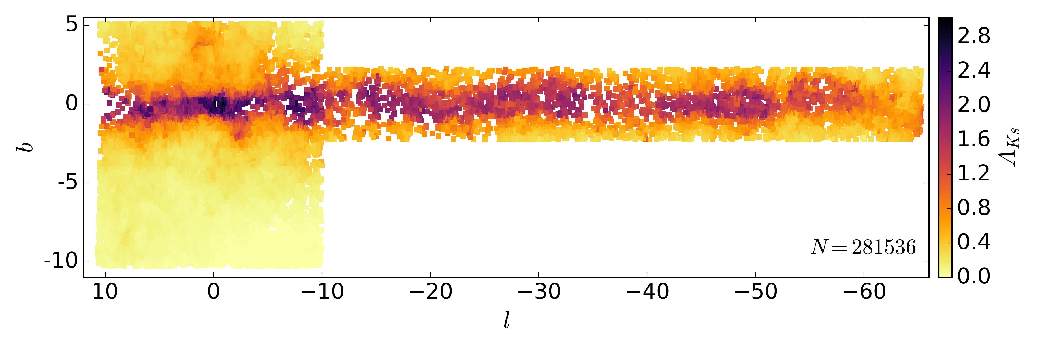
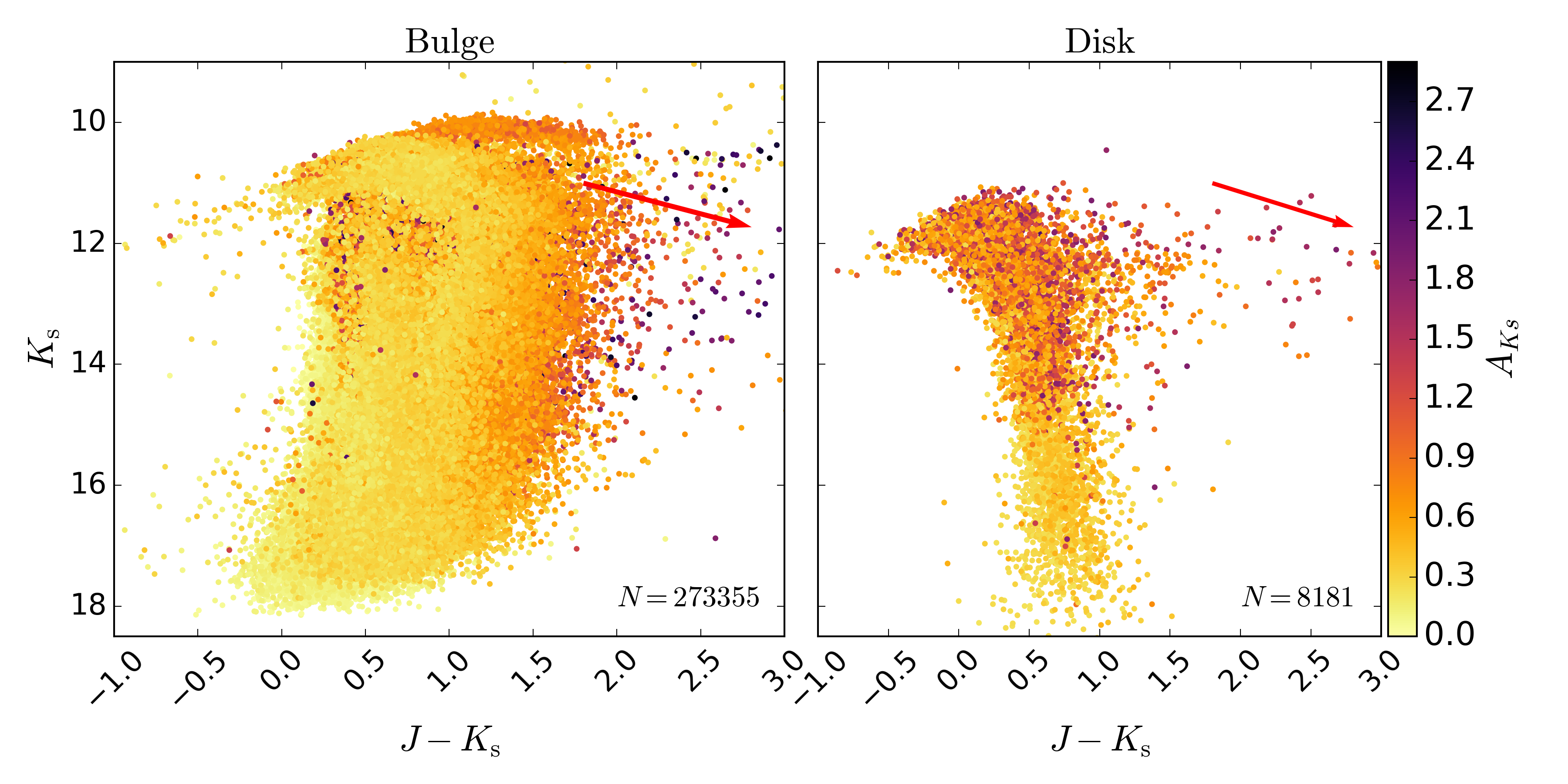
Figure 1: Top: Distribution for all 281 536 stars in the match VVV+VSX. The data points are colour-coded by the total extinction $A_{K\mathrm{s}}$, integrated along the entire line of sight for each object. Values vary from $A_{K{\rm s}}<0.01$ mag to $A_{K{\rm s}}\sim 3$ mag near the Galactic centre. For nearby objects the total extinction as calculated by the VVV maps is certainly overestimated. Bottom: CMD diagram for the bulge (left) and disk (right) containing the variable stars of our sample colour-coded by the $A_{K\mathrm{s}}$ parameter. The arrow shows the reddening vector for the diagram.

2.3 Cross-matching the VVV-VSX catalogue with Gaia-DR2

Recently, another huge database has been publicly released. It is the second data release (DR2) of the optical Gaia mission, which contains positional data for over one billion sources at $G$, $BP,$ and $RP$ bands, as well as precise parallaxes and proper motion measurements (Gaia Collaboration et al., 2018). The dataset allowed us to match the VVV+VSX and Gaia-DR2 catalogues, selecting the matches with the smaller separation within 1 arcsec radius. A total of 590 824 pairs were found within 1 arcsec, for which parallaxes are available in Gaia DR2 (we did not distinguish between positive and negative parallaxes because of the biases that this procedure would introduce in the sample, e.g. Bailer-Jones et al. 2018, BJ18 hereafter), and we can estimate the distance to them assuming a naive value of $d=1/\omega$. Distances based on Gaia parallaxes were also retrieved from BJ18, obtained on the basis of a three-dimensional model of the Galaxy instead of those obtained by simply inverting the parallax. From the total initial variables in our sample, we found 207 439 pairs for which BJ18 distances are available. A comprehensive description of distance estimates based on Gaia parallaxes is presented in Luri et al. (2018). The full description of all columns from Gaia that appear in the catalogue is given in Section 2.4.

Fig. 2 shows these resulting sources coloured by the $A_{K\mathrm{s}}$ as adopted for Fig. 1, but for the distances calculated from the Gaia parallax. Selecting only VVV sources whose $J$ and $K$s magnitudes have flags between -9 and 0 (see Section 2.1 for a more detailed overview of the meaning of the flags) and with the distance measured by BJ18, we obtain a sample containing 113 786 objects. The data we release contain all VVV+VSX matched variables, regardless of whether they are good according to the $JK_{\rm s}$ flag criteria. The discrepancy between the measured distance directly from the parallax and that from taken from BJ18 is quite evident. We can fairly assume that this correction is highly important because many of the Galactic sources in our sample would be located much farther away than they should when only considering the parallax, i.e. Galactic sources have distances bigger than the size of the Milk Way. Fig. 2 also shows the projected distribution of stars along with the height $z$ of the Galaxy as a function of the geometrical distance $y$. It is interesting to note that the stars appear to avoid the Galactic centre (around $b=0^{\circ}$), as is also visible in the spatial distribution of Fig. 1. This is a natural and known phenomenon and is the consequence of the high interstellar extinction along the line of sight of the disk and bulge.

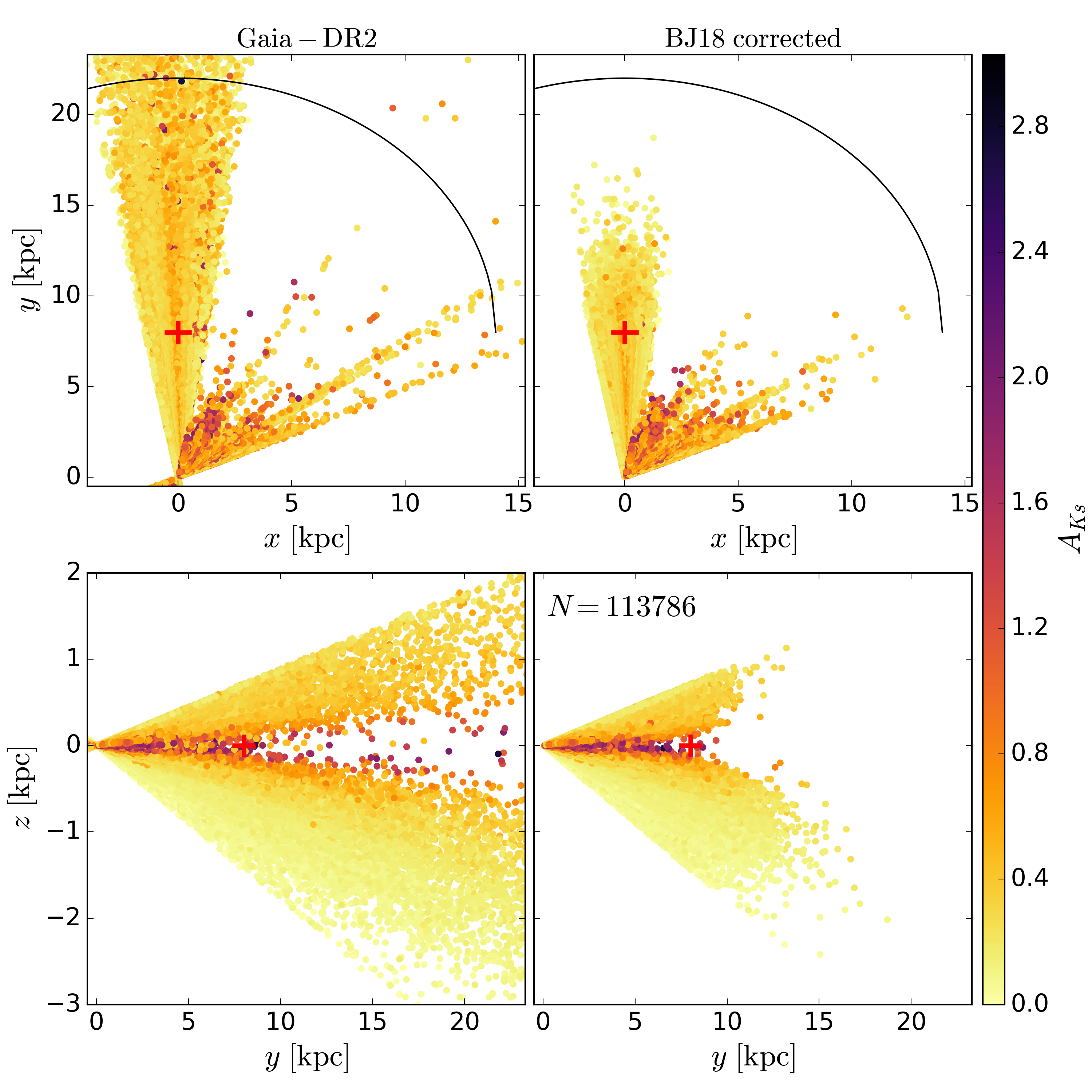
Figure 2: Distances calculated directly from the Gaia parallax (left) and distances from BJ18 (right). Upper panels: $(x,y)$ projection. The black semi-circle identifies the 15 kpc radius from the Galactic centre as a symbolic limit for the disk of the Galaxy. Lower panels: $(y,z)$ projection. The red cross identifies the geometrical position adopted to the centre of the Galaxy assuming $d=8$ kpc. The points are colour-coded by the total extinction in the $K$s band. The sample is constrained in the VVV $J$ and $K$s magnitudes and for those stars with distances measured using BJ18.

2.4 Column description

As Table 1 does not show many of the columns in our catalogue, in this section we describe all the columns from VVV that were modified or created by us that are available electronically as supplementary material (we do not describe those of the already public catalogues such as VSX and Gaia).

The following columns are directly obtained from the VVV catalogue:

• RA_(VVV) and DEC_(VVV): J2000.0 coordinates from the VVV catalogue (in degrees).

• L and B: The Galactic coordinates $l$ and $b$ as obtained for the VVV (in degrees).

• MAG_i: Magnitude of the sources measured by VVV, where $i=\left\{Z,Y,J,H,K\mathrm{s}\right\}$ are the respective bands of the VVV survey.

• ERR_i: Errors of the magnitudes of VVV to the respective bands $i=\left\{Z,Y,J,H,K\mathrm{s}\right\}$.

• F_i: The photometric flags for the bands where $i=\left\{Z,Y,J,H,K{\rm s}\right\}$.

The following columns are obtained from the information of VVV catalogue or from the complete match VVV+VSX+Gaia:

• $A_{Ks}$ : The total extinction in the $K$s  band.

• distance: Distances calculated using the Gaia parallax ($d=1/\omega$, in kpc).

• dist_BJ: Distances from BJ18 (estimated distance ‘r_est’, in kpc).

• (x,y,z)_BJ: Distances based on dist_BJ.

• CandidateType: Variables reclassified in Section 3.

The surface density distribution presented by the Fig. 3 is irregular and allows different interpretations in terms of stellar population and Galactic structure. For instance, a smaller number of objects is seen in the innermost bulge area. This so-called zone of avoidance is also present in the distribution of the VVV Novae catalogue (Saito et al., 2013) and is caused by the high extinction that affects the observations in the optical wavelengths, as seen in most variability surveys. This absence of objects in the innermost regions is even more evident in the distribution of long-period variable candidates from Gaia (Mowlavi et al., 2018), which is also based on optical observations. Observable objects in these regions are mainly from the foreground disk, as can be seen in the $y,z$ projected distances (bottom panels of Fig. 2). On the other hand, closer objects are probably saturated in the VVV observations and thus are not included in our sample.

The highest density of variable sources is seen in the intermediate bulge region ($-10\degree<b-5\degree$) of Fig. 3 and is mostly caused by RR Lyrae that were detected in variability surveys such as OGLE and VVV. Especially for OGLE, the footprint is easily seen across the bulge (see figure 7 in Soszyński et al., 2011). RR Lyrae are metal-poor population II stars that are detected in large numbers in the bulge region, compared to a small fraction that is present throughout the Galactic disk, which should be dominated by metal-rich population I stars (e.g. Dékány et al., 2018; Iorio & Belokurov, 2020).

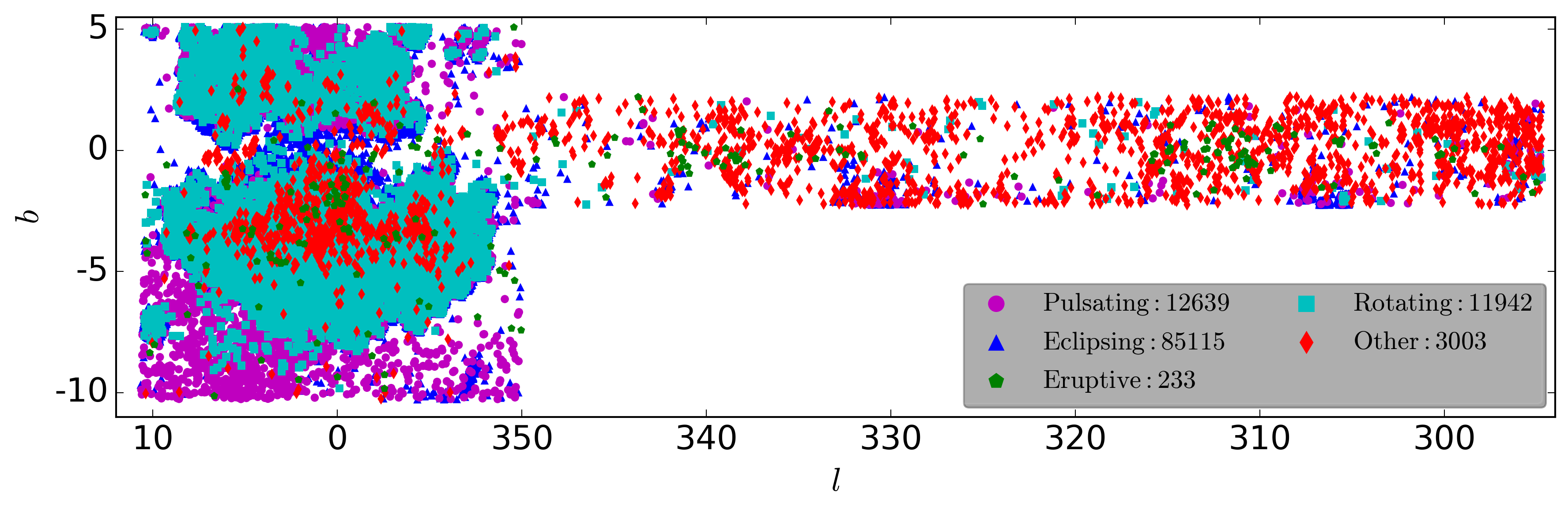
Figure 3: All 112 932 variables of our sample distributed through the five main classes we defined with the Galactic coordinates $l$ and $b$. Symbols are colour-coded following the legend in the figure.

2.5 Some statistics

This section is dedicated to gathering the information available for our VVV+VSX+Gaia catalogue. From the 701 256 variables in the match VSX+VVV, we selected all objects with flags lower than 0 and greater than -9 ( i.e. unsaturated point sources). We have the following numbers: 474 105 in $Z$ band, 420 775 in $Y$, 366 282 in $J$, 353 220 in $H$, and 346 614 in $K_{\rm s}$. There are 195 580 sources with good photometric quality in all five bands.

From the 590 824 objects with Gaia parallaxes, 206 624 have negative measures, with a minimum value of -443.735. These parallaxes are unreliable and hence were not used for any analysis involving distances, although the stars are not excluded from the table. The highest parallax value is for an M-type variable star in the bulge direction: 282.189 arcsec. For the positive values of the parallax, the mean value is 0.468 arcsec with a standard deviation ($\sigma$) of 0.990. The mean corresponding distance from the naive Gaia’s parallax is 28.326 kpc with $\sigma=1711.582$ kpc. For the BJ18 distances, the average is $\overline{d_{\rm BJ18}}=3.246$ kpc with $\sigma=1.625$ kpc.

2.5.1 Analysis of the VVV photo-flags

During the definition of the sample for the analysis of the VIVA catalogue, we realised that a considerable number of stars have flags 0 (noise) and 1 (non-stellar objects), but most of them are compatible and classified as point sources in VSX. We analysed the conditions of these measurements and briefly investigated whether they are misclassifications or spurious data. Fig. 4 shows the histograms of the stars (as identified in VSX) collected for these two flags. Out of 701 256, 2393 (0.34%) that were flagged as noise ($F\_K{\rm s}=0$) and are shown in the green histogram in Fig. 4, about half of them are fainter than the detection limit (the flag for the $K$s band is typically 17.5, although not constant, depending on the extinction of the region being considered). The right side of Fig. 4 shows the number of variables corresponding to each defined VSX class. For this analysis, all objects assigned as suspected variables in VSX (for which a colon is added to the class) were added to the group “Other”.

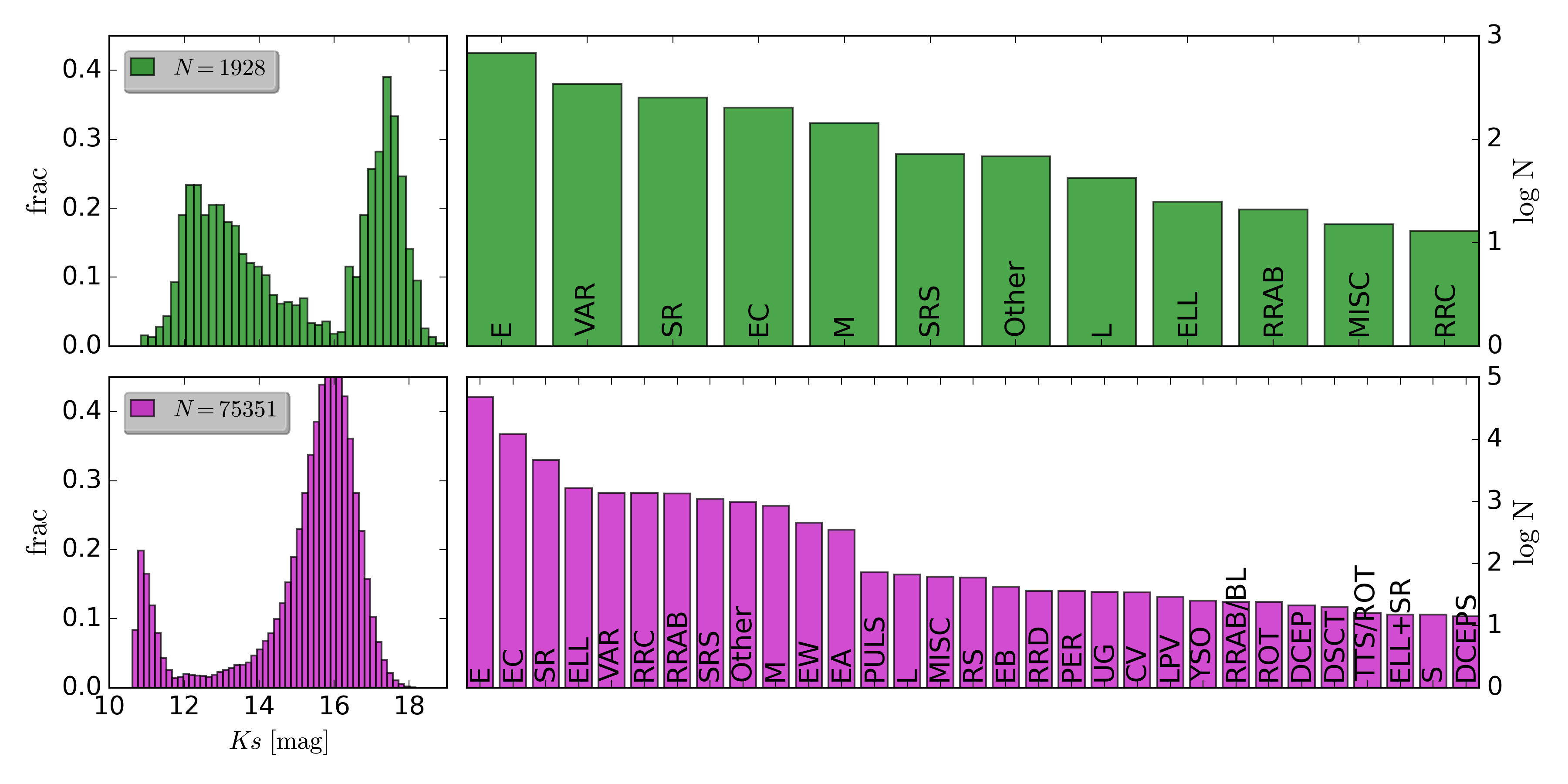
Figure 4: Green: Histogram (left) for the sources with flag 0 (noise) for the $K$s band and their distributions in the VSX classes (right side). Magenta: Same, but for flag 1 (non-stellar objects) for the $K$s band.

While flag 0 contains just a small number of objects, negligible for most purposes, flag 1 has a much more significant number of stars. We found that 133 808 (19%) stars in our main sample are classified as non-stellar objects. Fig. 4 shows the histogram and the distribution per variable class for these objects, and although part of the sample lies beyond (or very close to) the detection limit, these sources are better behaved, and most of them are within the saturation-detection limits. Moreover, most of the sources ($\sim 77$%) with $F\_Ks=1$ are eclipsing variables, with RR Lyrae and Mira following as second and third most common types in the sample.

We verified a similar behaviour for the other VVV bands ZYJH and find the same conclusions with similar numbers. This information can be further used to constrain their definitions and maybe improve the accuracy rate of these flags for future releases of the extended VVV survey (VVVX).

3 Variables through distance and period

As the number of different types of variables is high and thus prevents a clearer view in the diagrams, the similar variable types were merged following the VSX denomination for simplicity. We separated them into the five main groups following the definitions of the VSX for Eruptive, Rotating, Cataclysmic, Pulsating and Other, which contains all objects that are not included in the previous groups. The last group alone does not follow the VSX denomination strictly and might contain a mix of stars with unknown variability type and/or exotic sources such as active galactic nuclei, gama-ray bursts, quasars, and microlensing events. We did not add the composite types from VSX to these group (e.g. Algol systems, in which the low-mass component is close to its inner Roche lobe, EA/SD ), for instance.

We here then present some results using the period from VSX and other properties in terms of the five groups we just defined. For instance, we only used the $K$s magnitude and selected the good sources accordingly using only the flags in this band to constrain our sample. As a result, we have a higher number of variables, with a total of 130 855 objects, of which we show 129 938 in Fig. 5. The missing objects are stars that we were unable to classify into any of the five main classes defined here.

Fig. 5 shows the histograms normalised to 1 at their maximum for the defined classes of variables as a function of the distance calculated using the BJ18 distances. The Eruptive stars have two peaks at 1.3 kpc and 2.1 kpc, while the Other group exhibits a broad distribution from $\sim$0.5 kpc to $\sim$3 kpc and a tail extending up to 10 kpc. As this group contains different types of variables, this is an expected effect, possibly composed of a mix of Pulsating and Rotating stars. This assumption is being explored by other works.

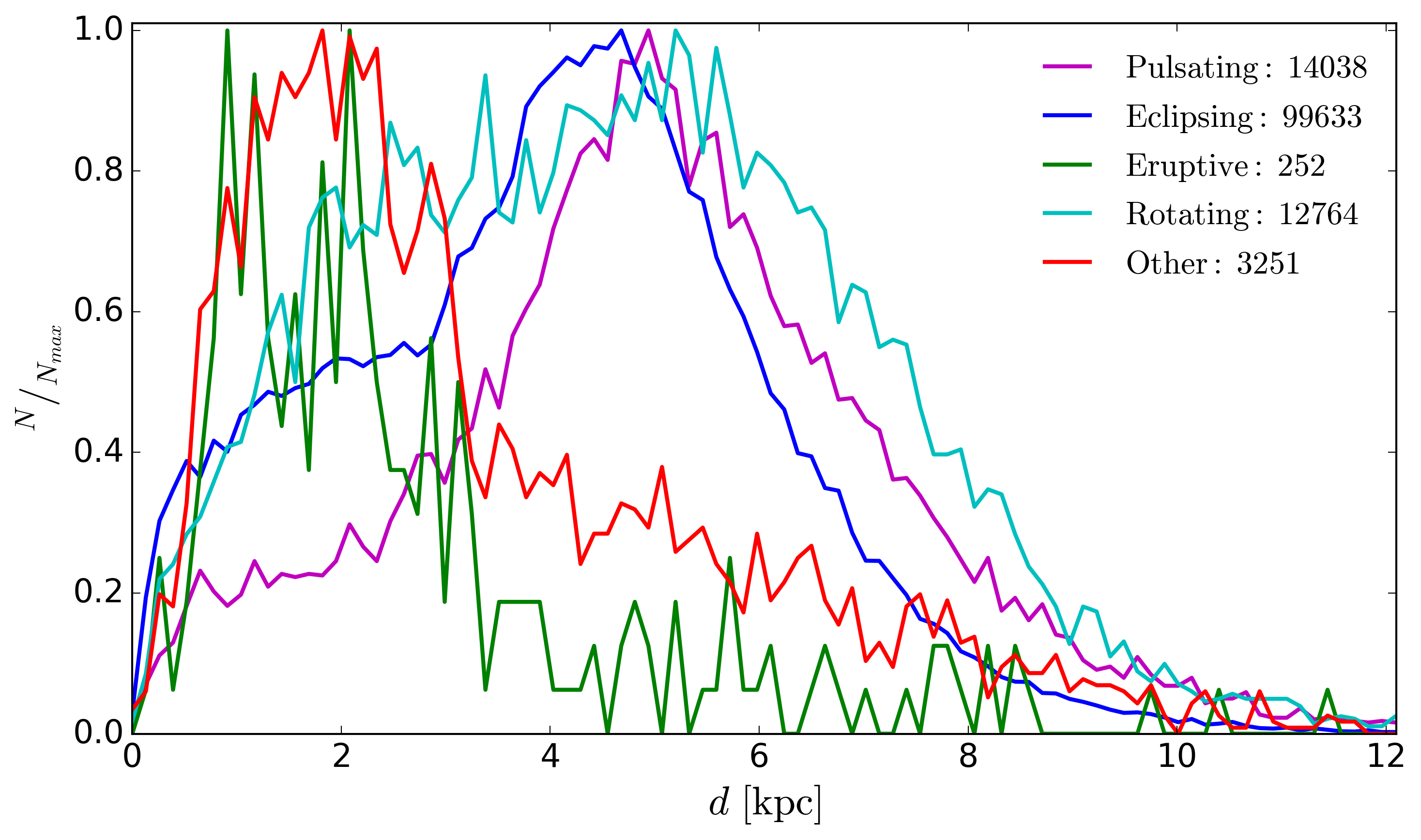
Figure 5: Histograms for the VSX classes of variables normalized to 1 relative to the distance calculated as in the Section 2.3.

Because exploring all the VSX classes, which are fundamentally related to our five main groups, is beyond of the scope of this work, we concentrated on one large group, the Pulsating stars, and three particular VSX types from the group Other. They are the VSX types MISC (stars whose classification was not precise enough with the automatic methods that were applied and they can be either red variables or irregular types stars), S (variables with rapid light changes that have not been studied so far), and VAR (unclassified variable stars).

The result of this selection are the 167 892 stars (here we introduce another cut to the sample because of the $A_{K\mathrm{s}}$ measurements, which cause 507 stars to be dropped from consideration) shown in Fig. 6 for the extinction-corrected $K$s magnitude ($K{\rm s}^{c}$) as a function of the BJ18 distance and colour-coded by the extinction $A_{K\mathrm{s}}$. We can identify five main groups: four horizontal groups ($K{\rm s}^{c}>16$, $K{\rm s}^{c}\sim 14.5$, $K{\rm s}^{c}\sim 12.5$, and $K{\rm s}^{c}<12$) for all distance ranges, and the fifth group, which spans from $9<K{\rm s}^{c}\lesssim 14$ but is concentrated at smaller distances ($d<3$ kpc).

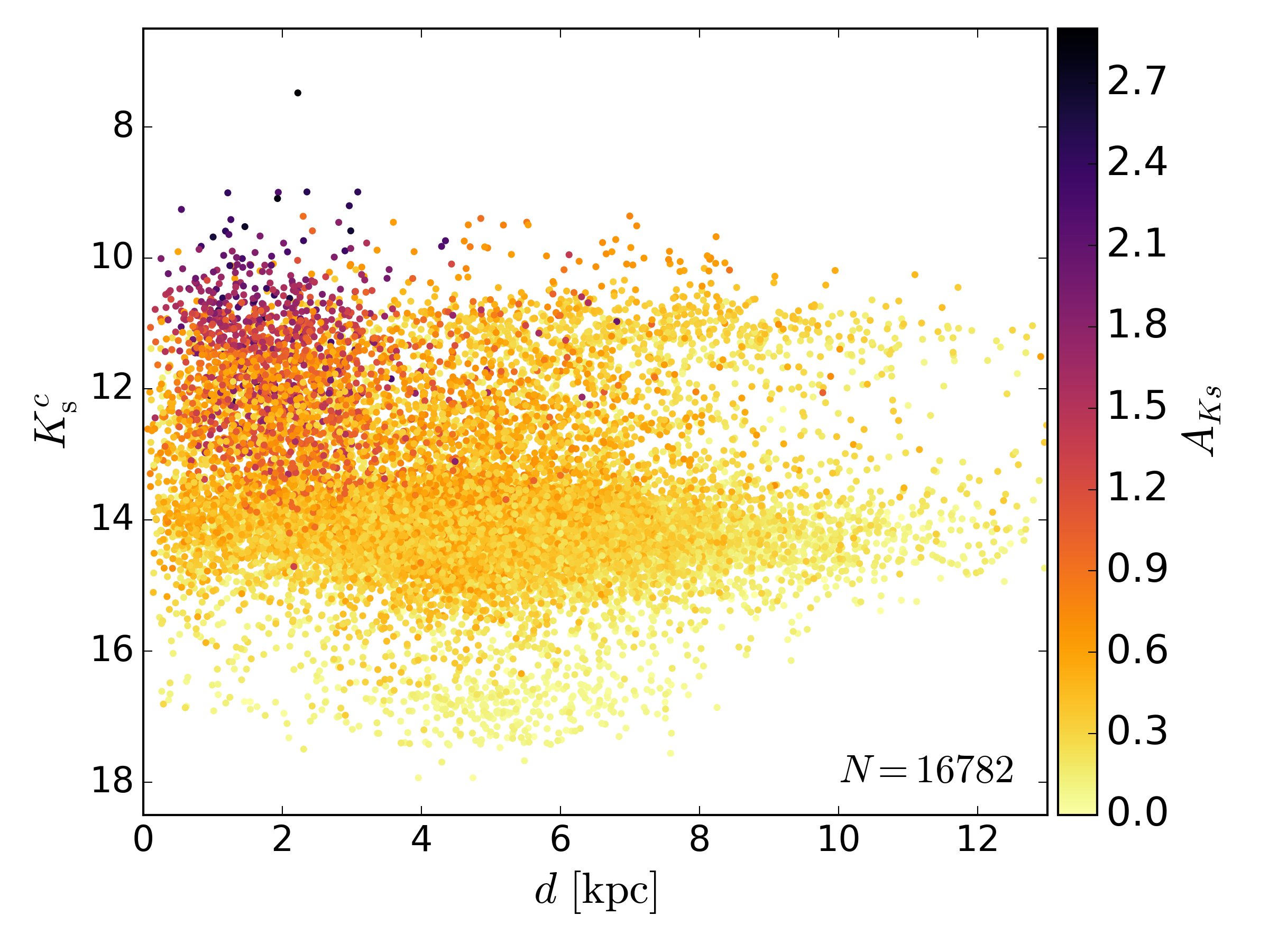
Figure 6: Distance of the group defined as Pulsating stars along with the VSX types MISC, S, UNC, and VAR from the group Other as a function of the extinction-corrected magnitude $K$s colour-coded by extinction $A_{K\mathrm{s}}$.

In the same manner, Fig. 7 shows the diagram of the period retrieved from the VSX catalogue as a function of the extinction-corrected $K$s magnitude for all variables shown in Fig. 6, except for those that do not have a measured period in the VSX catalogue for a total of 14 727 objects. The 2055 objects that are missing in this sample relative to those shown by Fig.  6 correspond to the stars with undetermined periods, and Fig. 6 and Fig. 7 show that they are mostly objects of high extinction that are mainly located at the centre of Galactic plane (see Fig. 1). Fig. 7 shows two dominant groups, most composed of RR Lyrae (shorter periods) and Cepheid stars (longer periods). We study the VSX classes individually in this projection.

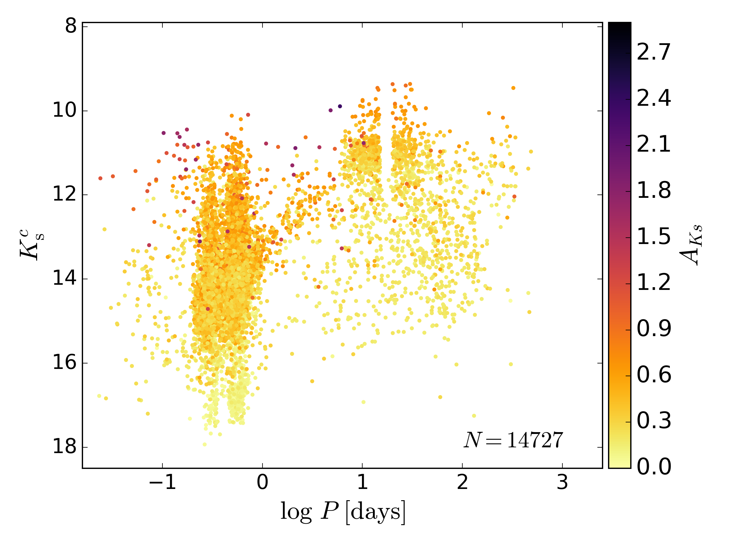
Figure 7: Extinction-corrected $K$s magnitude as a function of the period from the VSX catalogue, colour-coded by $A_{K\mathrm{s}}$.

To extend the study of Pulsating stars and the VSX variables types, we plot them in a diagram of magnitude $K$s (the apparent and the absolute) as a function of the period, but identifying the variable types that are considered (see Appendix B for the full names and descriptions of each type in Fig. 8). The results are shown in Fig. 8 along with the contours representing the $1\,\sigma$ boundary for the more populous groups. We easily identify two main distinct regions populated by RR Lyrae on one side and the semi-regular variables on the other. In between these two main groups lie the W Virginis variables (CWA and CWB), which occupy the upper portion of the diagram and several unstudied variables that occupy the lower portion (e.g. the unstudied variables with rapid light changes, S, form a well-defined group in this region along with other non-classified variables of the types MISC, PULS, and VAR).

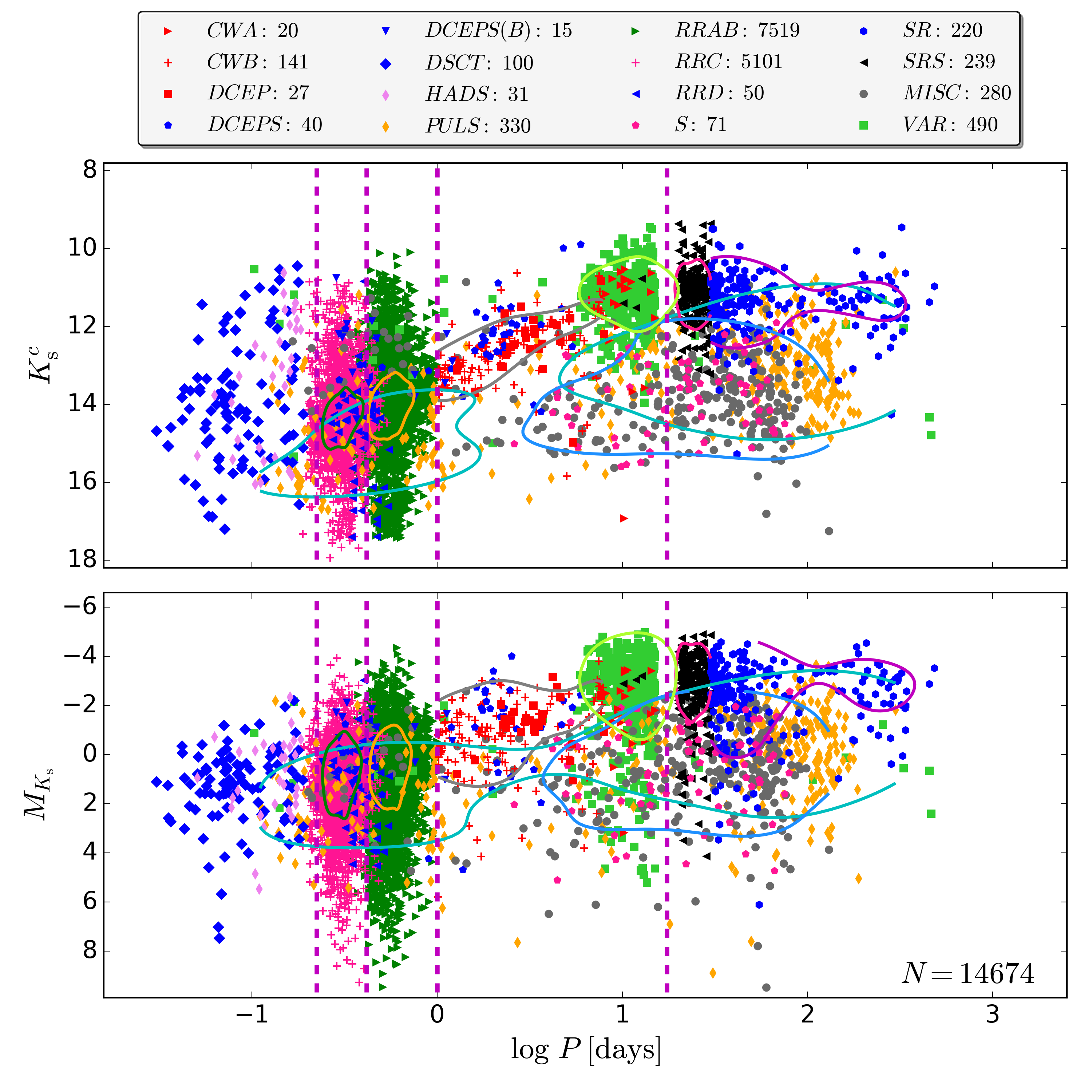
Figure 8: Diagram for the period as a function of the extinction-corrected $K$s (top panel) and absolute $M_{K{\rm s}}$ (bottom panel) magnitudes. The VSX variable types are highlighted. VSX types with fewer than ten stars were removed because they are not statistically relevant. The group called LPV (long-period variables) was removed because the measurement of its period in the VSX catalogue has low precision. Contours represent the 68th percentile (the contour colour differs from the point colour) of the types with more than 100 points and are represented as RRAB by the yellow contour, RRC in dark green, PULS in cyan, CWB in gray, MISC in blue, SR by the purple line, and VAR by the golden line. The vertical dashed purple lines represent the separation limits between DSCT and RRC ($\log\ P=-0.65$), RRC and RRAB ($\log\ P=-0.38$), above RRAB ($\log\ P=0$), and SR from short-period variables ($\log\ P=1.24$). The number $N$ in the bottom panel is the total number of variables shown.

The apparent magnitude of the types shown in Fig. 8 appears to be very well-defined in different regions of the diagram, they become more inhomogeneous when distributed over the period versus absolute magnitude plane, at least on the magnitude axis. We can still draw vertical lines in both panels of Fig. 8 using the contours as parameters for the divisor line. The first line is drawn at $\log\ P=-0.65$ and separates the $\delta$ Scuti type of variables (DSCT and HADS) from the RR Lyrae with symmetric light curves (RRC). The second line is located at $\log\ P=-0.38$ and separates the two RR Lyrae groups RRC and RRAB, the second being the RR Lyrae with asymmetric light curves. The third stands for all variables with higher periods than the RRAB and is positioned at $\log\ P=0$. Finally, the fourth line is drawn at $\log\ P=1.24$ and separates the semi-regular variables (SR) from those with shorter periods.

Based on these definitions, we can now identify the unclassified stars from our sample into the most populous VSX types, at least as a first approximation. We can then classify the types called MISC, PULS, and VAR depending upon which side of the lines they occupy. We did not classify type S when they occupy a region of the diagram that is not populated by any other well-defined VSX type in our sample (at $0<\log\ d<1.24$ and just below where the CWA, CWB, and SRS are located). They might be W Virginis or semi-regular pulsating variables or even more probably, they are variables other than pulsating stars and are to be classified accurately through other observations. We considered type S as a variability type of stars and included MISC, PULS, and VAR located at $0<\log\ d<1.24$ as S types. Our classification is loosely based on about two parameters: period and $K$s magnitude, and the term can be misread as a determination when in fact we intend to provide candidates that need to be studied in more detail to confirm their final type. Applying the definitions above (for the entire table) with good $K$s photometry and well-determined periods, we account for a total of 337 559 stars that are available for a reclassification, we find the number of candidates listed in Table 3. No PULS were considered. These results are included in the supplementary material as a new column in the table called CandidateType. We call attention to the stars of VAR type, however, which are by definition variables of undefined type. This nomenclature is also used for variable candidates, which makes the period found in the VSX database not completely reliable and implies that the strange gap around $\log\ P=1.24$ might be an artefact due to incorrect estimates of the period (we thank the anonymous referee for pointing this out). As a consequence, we must be careful when these stars are used for science. On the other hand, we consider them important objects to be targeted by variability surveys and/or follow-ups, therefore we kept them in the analysis of Fig. 8.

Table 3: Candidates to VSX variable types for the unclassified classes MISC, PULS, and VAR using the period vs. $K$s magnitude space from Fig. 8.

Type	DSCT	RRC	RRAB	S	SR
MISC	17	22	27	122	371
VAR	5	1	6	23 681	24

4 VIVA comparison

The VIVA catalogue (Ferreira Lopes et al., 2020) is based on a variability analysis of the VVV-DR4 Data Release that is the same as we used here. It was compiled following a series of recommendations in the New Insight into Time Series Analysis (NITSA - Ferreira Lopes & Cross, 2016b, 2017b; Ferreira Lopes et al., 2018). These criteria provide a good prescription for selecting variable stars. We caution that the VIVA catalogue only considered stars with more than ten non-flagged observations (number of good observations, or $\texttt{NG}>10$), that is, detection-flag (ppErBits) smaller than 256 and stack-flag (flag) equal to 0. The first is related to the archive curation procedures and the second to potential matching problems. These thresholds were adopted to reduce problems regarding the integrity of the detection. On the other hand, all VVV sources having at least one observation and at least one counterpart with VSX catalogue within an 1-arcsec radius are considered in V⁴SX.

By matching with V⁴SX within a radius of 1 arcsec, we found that 330838 single-detection point sources are not present in the VIVA catalogue. Three main reasons might be the origin of these differences: (a) our sample contains sources with fewer than ten non-flagged observations, (b) the signals reported in other wavelengths are not clear in the IR, and (c) the procedures used by Ferreira Lopes et al. (2020) fail. To understand these differences, we analysed the stars whose periods are reported in the literature, using the signal-to-noise ratio (S/N) estimated with harmonic fits to select our sample (e.g. Ferreira Lopes et al., 2015a, b).

We selected a sample of 10 793 stars considering two criteria: $\mathrm{S/N}>3$ and a number of good observations exceeding $20$ or $\mathrm{S/N}>2$ and NG higher than $100$. Following the VSX classification, this sample is composed mainly of eclipsing binaries ($\sim 63.5\%$), semi-regular variable stars ($\sim 23.5\%$), variables of unknown type ($\sim 8.4\%$), and RR Lyrae type stars ($\sim 3.2\%$). From these, we selected 1 195 sources by visual inspection of the phase diagram and light curve (side by side, as shown in Fig. 9). The flagged observations were also displayed to verify their weight on the data. During this process, we observed many objects that appeared to be similar to Algol-type stars, whose periods might be inaccurate (Carmo et al., 2020), as well as some that appeared to have a very low amplitude signal.

On the other hand, for the selected objects displaying good signals (for which three examples are shown in Fig. 9), we observed that $\sim 98\%$ of them belong to the VVV bulge fields. These regions are more crowded and dustier than those located in the disk area, and as a consequence, the number of missed sources is expected to be higher. Additionally, noting that the peak of the magnitude distribution of our sample is at $K{\rm s}\sim 15$ mags, the missed sources are in general faint objects with a low S/N (see middle panel of Fig. 9). These correspond to less than $0.5\%$ of the variable stars with more than ten non-flagged observations. We also observed that some flagged observations may be useful for identifying LPVs (see the top diagrams in Fig. 9). Only the LPVs appear to show variability at the flagged measurements. On the other hand, the flagged observations might also indicate the zero-point error (see the middle panels in Fig. 9). We caution that these observations must be used carefully because they can also increase the noise of the signal.

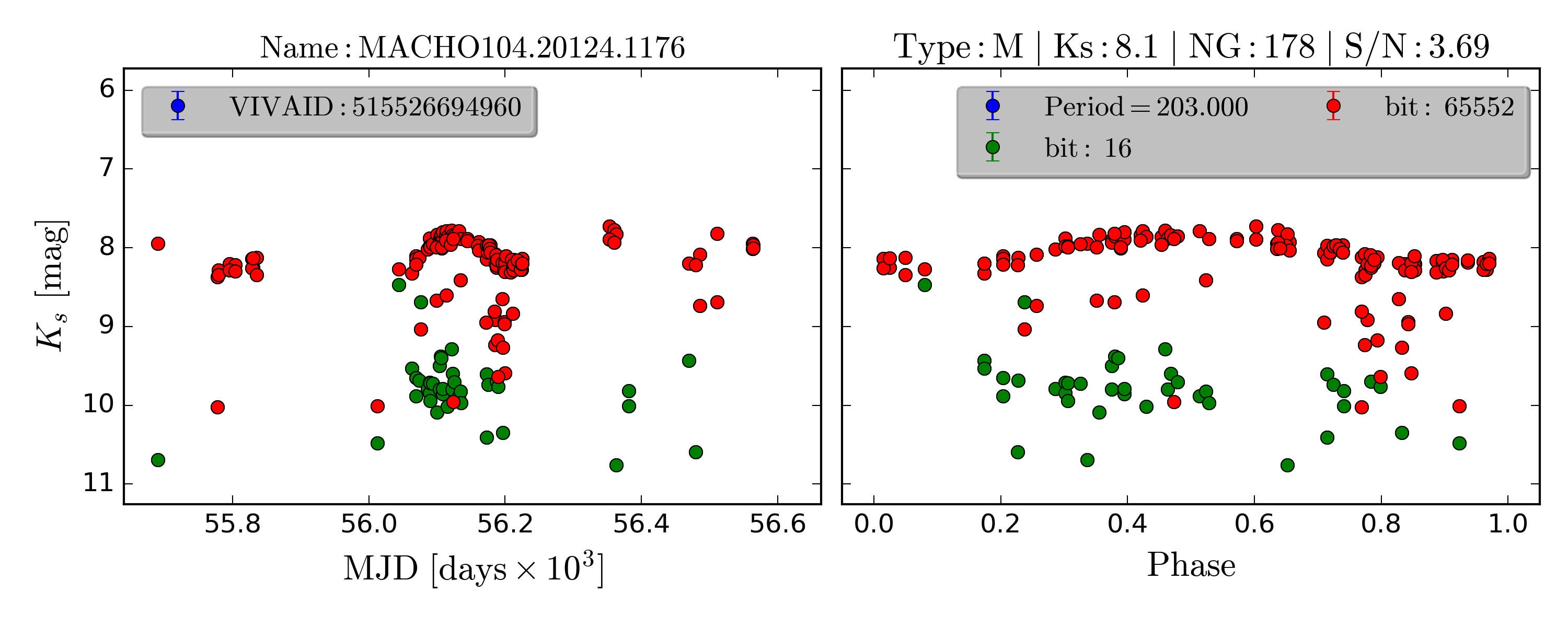
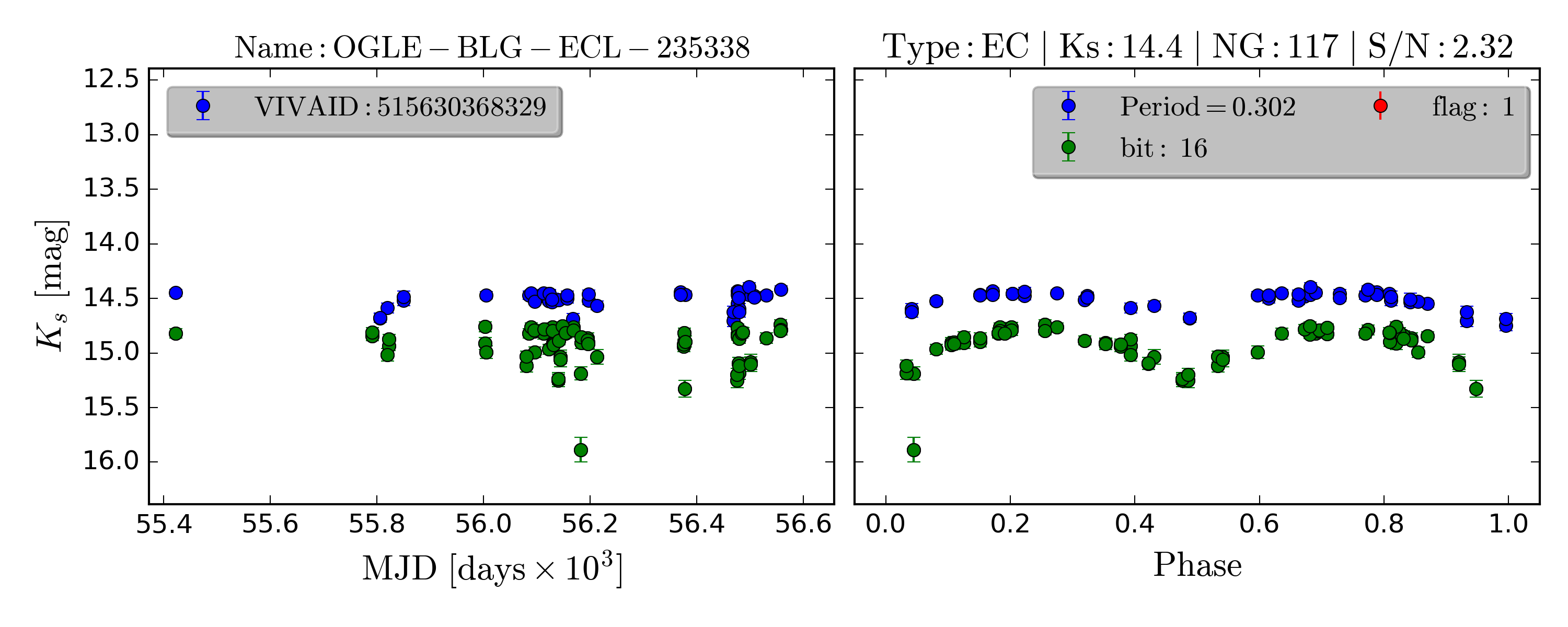
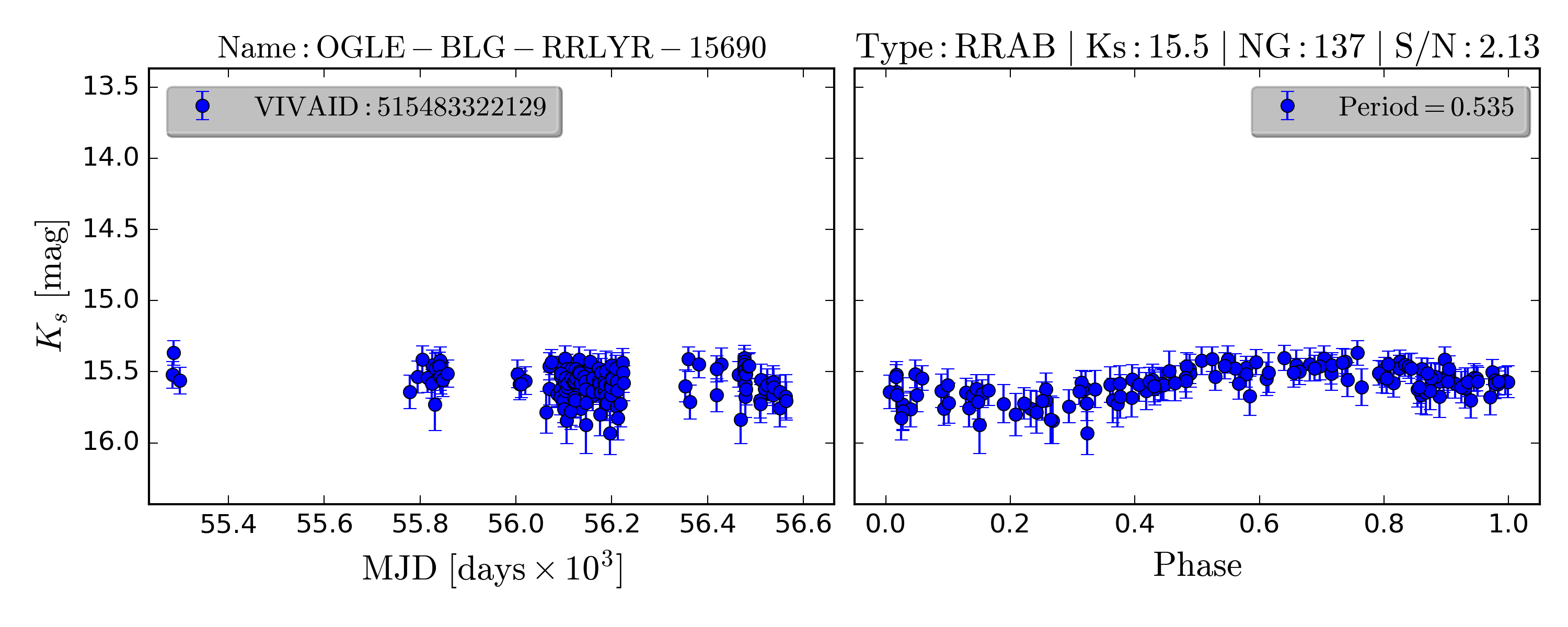
Figure 9: Time domain (on the left side) and phased light curves (on the right side) for examples of variable stars that are missing in the VIVA catalogue. The light curves display the VSX nameat the top and the VIVA ID inside the legend box, and the corresponding phase diagram shows the VSX type (Type), the VVV $K$s magnitude, the number of good observations NG, and the S/N estimated with harmonic fits at the top, with the VSX period and the ppErrbits flags in the legend box inside the diagram. Blue points represent $\texttt{ppErrbits}=0$ for good observations, and red and green stand for observations with $\texttt{ppErrbits}\neq 0$.

In summary, our results agree with those of Ferreira Lopes et al. (2020), that is, the VIVA catalogue includes about $99\%$ of all variable stars found in the VVV Data Release 4 that have good signal. The missed sources correspond to faint stars mainly with a low S/N. Additional observations from VVVX can help solve this matter. Moreover, Hajdu et al. (2020) identified two independent types of bias in the photometric zero-points in VVV data that can also improve the data quality.

5 Conclusions

We presented a near-infrared catalogue that includes accurate individual coordinates, magnitudes, and extinctions as well as distances based on Gaia parallaxes for variable stars presented in the VSX catalogue and also in the VVV near-infrared colour catalogue. Our CMDs, colour-colour diagrams, and surface density distributions for the different types allow us to give a global characterization of Galactic variables stars, including important distance indicators such as RR Lyrae, Cepheids, abd Miras.

Our results suggest that the current knowledge of variability in the Galaxy is biased to nearby low extinct stars and that therefore the larger part of the Galaxy disk and bulge is still unexplored by stellar variability studies.

We provide a set of several thousand candidates to different VSX types of variables using the period space to constrain the region they occupy in the period versus magnitude diagram. This result can be used to target specific samples of stars to determine the characteristics through follow-up campaigns.

Future studies of the Milky Way variable stars will be revolutionised by the LSST survey in the next decade, for which the discovery of hundreds of thousands of variables is expected. Thus, the present catalogue also provides the groundwork to characterise the results of future projects. Another important aspect to consider is the near-infrared versus optical variability. The searches performed at different wavelengths result in different relative numbers of variables, and this must be considered when the number of Rubin Observatory findings in this field is predicted (e.g. Pietrukowicz et al., 2012).

Near-infrared surveys such as the VVV are efficient at low Galactic latitudes close to the plane, where optical surveys are usually blinded by the absorption in the interstellar medium. In the same way that Baade’s Window was important for optical studies of the Galactic bulge, the near-infrared surveys also profit from the study of the windows that have recently been found in the Milky Way plane (Minniti et al., 2018).

By analysing the photometric flags from the VVV catalogue, we identified a misclassification regarding noise and mainly non-stellar objects. These stars are misclassified even inside the magnitude range that allows a good verification of the data and typically corresponded to $\sim$20% of our sample for all VVV bands.

Additionally, we identified a considerable number of variables inside our sample that were missed during the selection of the VIVA catalogue. They are mostly sources with low signal-to-noise ratio, stars with photometric problems, and for about 1% of them, the procedure used to identify the variability failed. These sources can help to improve the variability analysis of the VVV survey and to verify the accuracy of the VVV photometric flags. This information is valuable to improve the procedures and completeness of future releases.

Appendix A Merged classes and what they contain

In this section we list all VSX types that were merged into the five large classes discussed in Section 3. The classes include the following types:

• Eclipsing: E, EA, EB, EP, EW, EC, ED, ESD, AR, D, DM, DS, DW, EL, GS, HW, K, KE, KW, PN, SD, WD.

• Rotating: ACV, BY, CTTS/ROT, ELL, FKCOM, HB, LERI, NSIN ELL, PSR, R, ROT, RS, SXARI, SXARI/E, TTS/ROT, WTTS/ROT.

• Pulsating: ACEP, ACYG, AHB1, (B), BCEP, BCEPS, BL, BLAP, BXCIR, CEP, CW, CWA, CWB, CWB(B), CWBS, GWLIB, CW-FO, CW-FU, DCEP, DCEP(B), DCEPS, DCEPS(B), DCEP-FO, DCEP-FU, DSCT, DSCTC, DSCTr, DWLYN, GDOR, HADS, HADS(B), L, LB, LC, LPV, M, O, PPN, PULS, PVTEL, PVTELI, PVTELII, PVTELIII, roAm, roAp, RR, RRAB, RRC, RRD, RV, RVA, RVB, SPB, SR, SRA, SRB, SRC, SRD, SRS, SXPHE, SXPHE(B), V361HYA, V1093HER, ZZ, ZZA, ZZB, ZZ/GWLIB, ZZO, ZZLep.

• Eruptive: BE, cPNB[e], CTTS, DIP, DPV, DYPer, EXOR, FF, FSCMa, FUOR, GCAS, I, IA, IB, IN, INA, INAT, INB, INS, INSA, INSB, INST, INT, IS, ISA, ISB, RCB, SDOR, TTS, UV, UVN, UXOR, WR, WTTS, YSO, (YY), ZZA/O.

• Other: Includes all Cataclismic Variables (AM, CBSS, CBSS/V, CV, DQ, IBWD, N, NA, NB, NC, NL, NL/VY, NR, S, SN, SN I, SN Ia, SN Iax, SN Ib, SN Ic, SN Ic-BL, SN II, SN IIa, SN IIb, SN IId, SN II-L, SN IIn, SN II-P, SN-pec, UG, UGER, UGSS, UGSU, UGWZ, UGZ, UGZ/IW, V, V838MON, VY, ZAND), X-Ray (BHXB, HMXB, IMXB, LMXB, X, XB, XBR, XJ, XN, XP, XPR), and other objects (AGN, APER, BLLAC, CST, GRB, Microlens, MISC, non-cv, NSIN, PER, QSO, S, SIN, Transient, UNC, VAR, VBD).

Appendix B Summary of VSX classes

In this section, we list the main features of a few types of variables used in Section 3 along with the full names for all variability classes shown by Fig. 8. The descriptions are taken from the VSX index.

• BCEP : $\beta$ Cephei type variables.

• CWA: W Virginis variables with periods longer than eight days.

• CWB: W Virginis variables with periods shorter than eight days (also known as BL Herculis variables).

• DCEP: Classical Cepheids

• DSCT : Variables of the $\delta$ Scuti type.

• HADS: High-amplitude $\delta$ Scuti stars.

• M: o (omicron) Ceti-type (Mira) variables.

• MISC: Miscellaneous variables stars. Usually red variables (L or SR) or other types of irregular stars, I or BE) that cannot be classified more specifically by the automatic analysis made in the surveys.

• PULS: Pulsating variables of unspecified type.

• RR: Variables of the RR Lyrae type.

• RRAB: RR Lyrae variables with asymmetric light curves, periods from 0.3 to 1.2 days, and amplitudes from 0.5 to 2 mag. in V.

• RRC: RR Lyrae variables with nearly symmetric sometimes sinusoidal light curves, periods from 0.2 to 0.5 days, and amplitudes not greater than 0.8 mag. in V.

• RRD: Double-mode RR Lyrae stars that pulsate in the fundamental mode as well as in the first overtone with a period ratio of 0.74 and a fundamental period near 0.5 days.

• RV: Variables of the RV Tauri type.

• RVA: RV Tauri variables that do not vary in mean magnitude.

• S: Unstudied variables stars with rapid light changes.

• SPB: Slowly pulsating B stars showing both light and line profile variability.

• SR: Semi-regular variables, which are giants or supergiants of intermediate and late spectral types showing noticeable periodicity in their light changes, accompanied or sometimes interrupted by various irregularities.

• SRA: Semi-regular late-type (M, C, and S or Me, Ce, and Se) giants displaying persistent periodicity and usually small (¡2.5 mag. in V) light amplitudes.

• SRB: Semi-regular late-type (M, C, and S or Me, Ce, and Se) giants with poorly defined periodicity (mean cycles in the range of 20 to 2300 days) or with alternating intervals of periodic and slow irregular changes, and even with light constancy intervals.

• SRS: Semi-regular pulsating red giants with short periods (several days to a month), probably high-overtone pulsators.

• VAR: Variables stars of unspecified type.