Transverse loop oscillations via vortex shedding: a self oscillating process

Abstract

Identifying the underlying mechanisms behind the excitation of transverse oscillations in coronal loops is essential for their role as diagnostic tools in coronal seismology and their potential use as wave heating mechanisms of the solar corona. In this paper, we explore the concept of these transverse oscillations being excited through a self-sustaining process, caused by Alfvénic vortex shedding from strong background flows interacting with coronal loops. We show for the first time in 3D simulations that vortex shedding can generate transverse oscillations in coronal loops, in the direction perpendicular to the flow due to periodic “pushing” by the vortices. By plotting the power spectral density we identify the excited frequencies of these oscillations. We see that these frequencies are dependent both on the speed of the flow, as well as the characteristics of the oscillating loop. This, in addition to the fact that the background flow is constant and not periodic, makes us treat this as a self-oscillating process. Finally, the amplitudes of the excited oscillations are near constant in amplitude, and are comparable with the observations of decay-less oscillations. This makes the mechanism under consideration a possible interpretation of these undamped waves in coronal loops.

1 Introduction

In recent years, observations by the Coronal Multi-channel Polarimeter, the Solar Dynamics Observatory, and Hinode spacecraft have already proven the ubiquity of transverse perturbations and waves in magnetic structures in the solar corona (e.g. Tomczyk et al., 2007; McIntosh et al., 2011). The importance of these waves and oscillations is connected to their use in coronal seismology (e.g. Nakariakov & Ofman, 2001; Nakariakov & Verwichte, 2005), as well as their potential role as heating mechanisms for the solar corona (for a review, see Van Doorsselaere et al., 2020).

Kink oscillations of coronal loops have been intensively studied ever since they were firstly observed (Aschwanden et al., 1999; Nakariakov et al., 1999). Following the theory of waves in a magnetized cylindrical flux tube (Zajtsev & Stepanov, 1975; Edwin & Roberts, 1983), these observed perturbations have been treated as standing kink modes (Van Doorsselaere et al., 2008). These first observations were of oscillations with amplitudes of a few megameters, which were decaying over time after an being excited by external energetic phenomena (e.g. Nakariakov et al., 1999; Zimovets & Nakariakov, 2015; Nechaeva et al., 2019). The damping of these oscillations has been attributed to the phenomena of resonant absorption and phase mixing (Ionson, 1978; Heyvaerts & Priest, 1983; Goossens et al., 2011) and have been studied both analytically and numerically in 3D MHD setups, where the effects of gravity, radiation, and the Kelvin-Helmholtz instability (KHi) has also been considered (e.g. Terradas et al., 2008; Antolin et al., 2014; Magyar et al., 2015; Hillier et al., 2019).

Alongside those larger-amplitude decaying oscillations, a second category of low-amplitude, transverse waves occurring in coronal loops has also been observed in recent years. These waves were first detected by Wang et al. (2012) and Tian et al. (2012), and were proven to be omnipresent in active region coronal loops (Anfinogentov et al., 2013, 2015), making them possible tools for coronal seismology (Anfinogentov & Nakariakov, 2019; Yang et al., 2020). These decay-less oscillations have a near constant amplitude over the course of many periods, with frequencies equal to that of the fundamental standing kink mode (Nisticò et al., 2013), as well as its second harmonic (Duckenfield et al., 2018).

While the mechanism exciting these decay-less oscillations is still not identified, different explanations have been studied over the years. In Antolin et al. (2016), they were treated as line-of-sight effects created by the KHi vortices from impulsively oscillating coronal loops. Decay-less oscillations have also been modeled numerically as driven standing waves from footpoint drivers, both from monoperiodic (e.g. Karampelas et al., 2017, 2019; Afanasyev et al., 2019; Guo et al., 2019; Shi et al., 2021) and broadband drivers (Afanasyev et al., 2020). Another interpretation was considered in Nakariakov et al. (2016), in the form of a self-sustained oscillation. Unlike periodically driven oscillations, where the input of energy is done periodically and the frequency is imposed by the driver, self-oscillations are excited from (near) constant drivers, and the oscillation frequency is set by the system itself, and not the external driver. In short, self-oscillations are processes that can turn a nonperiodic driving mechanism into a periodic signal. Such a process was modeled in Karampelas & Van Doorsselaere (2020), where a slow constant flow around a loop’s footpoint eventually led to the excitation of a weak oscillation. Despite the numerical limitations, that study has provided a first proof-of-concept for this process in a 3D simulation.

In the current work we will continue to explore the concept of self-oscillations of coronal loops, by considering the excitation of a transversely polarized wave through the mechanism of Alfvénic vortex shedding. Evidence of vortex shedding in the solar corona was reported in Samanta et al. (2019), in the vicinity of a shrinking loop in a post-flare region. Vortex shedding due to solar wind has also been proposed by Nisticò et al. (2018), to explain the observed oscillations of cometary plasma tails. In a 0D model first proposed by Nakariakov et al. (2009), it was described how vortices generated by an upflow passing by a loop can excite an oscillation through a quasi-periodic horizontal force. The phenomenon of Alfvénic vortex shedding has already been explored numerically for a bluff body in 2D in Gruszecki et al. (2010). However, a coronal loop will behave differently than a fixed and rigid bluff body, thus making a 3D study essential. In this work we will study for the first time the excitation of kink-mode oscillations by vortex shedding for a full 3D setup of a coronal loop. We will focus on the decay-less regime, although this method can also be applied to decaying oscillations. We will show that the mechanism under consideration can be a possible interpretation of these undamped loop oscillations. Finally, we will explore how this mechanism is affected by the characteristics of both the flow and the oscillator, making it essentially a self-oscillation that can be initiated in solar coronal loops.

2 Numerical setup

We use a model of a straight flux tube of (minor) radius $R=1$ Mm and length $L=200$ Mm. This model corresponds to a semicircular coronal loop with a major radius or $\sim 64$ Mm. The radial density profile for our model is given by the relation

$$\rho(x,y)=\rho_{e}+(\rho_{i}-\rho_{e})\zeta(x,y),$$ (1)

$$\zeta(x,y)=0.5(1-\tanh((\sqrt{x^{2}+y^{2}}/R-1)\,b)),$$ (2)

where $b$ sets the width of the boundary layer. We consider $b=20$, which gives us an inhomogeneous layer of width $\ell\approx 0.3R$. The index $i(e)$ corresponds to the internal (external) values with respect to our flux tube. The coronal background (or external) density is equal to $\rho_{e}=0.836\times 10^{-12}$ kg m^-3, three times lower than the loop (internal) density ($\rho_{i}$). Similarly to Karampelas & Van Doorsselaere (2020), the temperature varies across the tube axis (in the $xy$-plane), ranging from $0.9$ MK inside the loop to $1.35$ MK outside (see Figure 1), effectively modeling a loop during a cooling phase, as observed for loops in thermal nonequilibrium (Froment et al., 2017). The scale height for our model ($H\sim 55$ Mm) is comparable to the major radius or the corresponding coronal loop, which allows us to approximate the temperature as constant with height, along the flux tube. For our primary setup, we consider a straight magnetic field $B_{z}$, parallel to the loop axis ($z$-axis) with internal and external field values of $B_{zi}=22.8$ G and $B_{ze}=22.9$ G respectively. The magnetic field distribution is set in such a way that it maintains a total (magnetic + gas) pressure balance across our domain. This prevents any unwanted perturbations from developing at the start of the simulation.

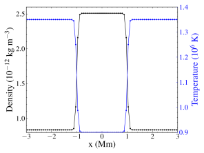
Figure 1: Density (in black) and temperature profile (in blue) of the flux tube cross-section along the $x$-axis at time $t=0$. The grid points are depicted as dots on the two curves.

Our setup has domain dimensions of $x\in[-7,17]$ Mm, $y\in[-20,20]$ Mm and $z\in[-100,100]$ Mm, with a resolution of $(\delta x,\delta y,\delta z)=(80,80,2000)$ km. The loop footpoints are placed at positions $z=-100$ and $z=100$ Mm, while $z=0$ is the location of the loop apex. This resolution allows us to study the motion of the loop and the development of larger scale flow instabilities, like vortex-shedding, in the $xy$-plane.

The side boundaries in the $y$ direction, as well as at $x=17$ Mm are set to have Neumann-type, zero-gradient conditions for all quantities. On the “left” side boundary (at $x=-7$ Mm), we apply zero-gradient conditions for the pressure and density, the three components of the magnetic field, and the $v_{y}$ and $v_{z}$ components of the velocity field. For the $x$ velocity component at $x=-7$ Mm, we apply a fixed value of $v_{x}=5\times 10^{4}$  m s^-1, for a total duration of $\Delta t=1012$ s. This leads to the development of a horizontal flow along the $x$ direction, which is also free to evolve along the $y$ direction as well (see Figure 2). After a time $t=1012$ s we switch the boundary condition for $v_{x}$ at $x=-7$ Mm to zero-gradient, letting the initiated flow to evolve freely.

At the “bottom” and “top” boundaries ($z=-100$ and $z=100$ Mm), we apply zero-gradient conditions for the pressure, density, and the three components of the magnetic field. The $v_{z}$ velocity component (along the axis of the loop) is set as antisymmetric, to prevent any outflows from the top and bottom boundaries, where the bases of the loop are located. Inside the loop ($\sqrt{x^{2}+y^{2}}\leq R$), the $v_{x}$ and $v_{y}$ are set as antisymmetric, to fix the loop endpoints. Outside the loop at $z=-100$ and $z=100$ Mm we set the $v_{x}$ and $v_{y}$ components as zero-gradient (outflow conditions) in order to let the flow evolve freely along the $xy$-plane, in a way that allows for the development of vortices.

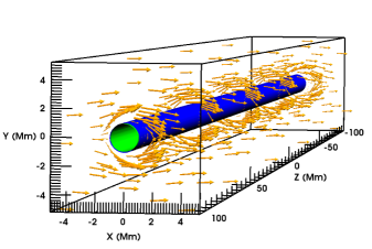
Figure 2: Schematic representation of the flow along the $x$ direction, originating from the “left” side boundary at $x=-7$ Mm (not shown here).

All calculations were performed in ideal MHD in the presence of numerical dissipation, using the PLUTO code (Mignone et al., 2012). We use the second-order characteristic tracing method to calculate the timestep, and the finite volume piecewise parabolic method (PPM) with a second-order spatial global accuracy and the Roe solver. Finally, to keep the solenoidal constraint on the magnetic field, we employ Powell’s $8$-wave scheme.

3 Results

Following the basic idea from Nakariakov et al. (2009), we try to model an upflow around a coronal loop, originating from the propagation of a CME. To that end, we initiate a flow from one of the side boundaries (at $x=-7$ Mm) for a duration of $t=1012$ s or $t=4\cdot P$, where $P=253$ s is the period of the fundamental kink mode (Edwin & Roberts, 1983) for a loop with the characteristics of our primary setup, as described in Section 2. A schematic representation of that flow, is shown in Figure 2. Driving with a constant background flow, equal for all heights, is a rather unlikely physical scenario, which can render a straight flux tube unstable. This is due to the strong excitation of higher harmonics due to the spatial profile of the flow over the loop height. To prevent this, we “switch off” the side boundary driver for $t>1012$ s and replace it with a zero-gradient boundary condition at $x=-7$ Mm. This allows the flow to evolve freely through its interaction with the loop.

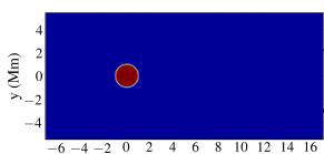
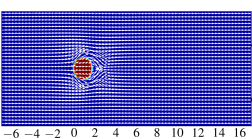
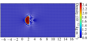
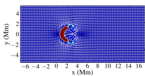
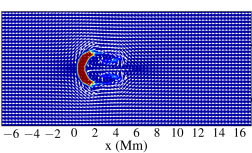
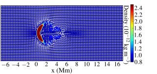
Figure 3: Contour plots of density ($\times 10^{-12}$ kg m^-3) for our loop, at the apex. The velocity field is also overplotted. From left to right, starting from the top panels, we show the contours at the first six snapshots of the simulation, between $t=0$ and $t=189.8$ s, for every $31.62$ s. An animation of the density evolution is included in the online version of this manuscript.

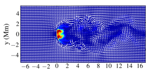
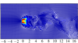
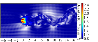
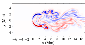
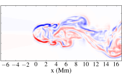
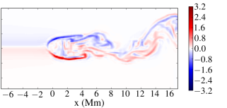
Figure 4: Top panels: contour plots of density ($\times\,10^{-12}$ kg m^-3) for our loop at the apex, with the overplotted velocity field in white. Bottom panels: contour plots of the plasma $z$-vorticity ($\times\,0.1285$ Hz) for our loop at the apex. From left to right, snapshots are shown at $t=1012$, $1265$ and $1518$ s. An animation of the $z$-vorticity ($\omega_{z}$) evolution is included in the online version of this manuscript.

The phenomenon of Alfvénic vortex shedding was studied in 2D for a coronal environment in Gruszecki et al. (2010). In that study, a bluff (fixed and rigid) body was introduced in the path of a uniform plasma flow, initiating vortex shedding. The hydrodynamical relation for the Strouhal number (St) was tested, which is a dimensionless parameter depending on the period ($P$) of the vortex shedding, the size (here diameter, $d$) of the blunt body and the flow velocity ($V_{0}$):

$$St=\frac{d}{PV_{0}}.$$ (3)

In Gruszecki et al. (2010) it was found that the Strouhal number in MHD for coronal parameters has values between $0.15$ and $0.25$. Considering a loop with diameter $d=2$  Mm (minor radius of $1$  Mm) and a period for the fundamental kink-mode equal to $253$ s, flow speeds of $V_{0}\sim 30-50$ km s^-1 would be required for the initiation of vortex shedding with the same periodicity. This would be essential in order for the loop to resonate with and be driven by the vortices. Assuming an average value of St$\sim 0.2$ for the Strouhal number, we chose to initiate a flow from the side boundaries with a velocity of $v_{x}=V_{0}=50$ km s^-1, in order to excite an oscillation with a frequency close to that of the fundamental kink mode.

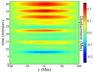
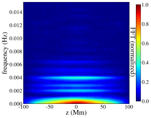
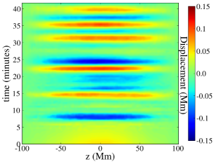
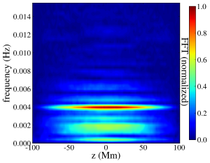
Figure 5: Left panels: displacement of the loop center of mass at each height, for the duration of the simulation. The top panel is for the full time-series, and the bottom panel is for the detrended time series. Right panels: the corresponding normalized power spectral density plots for the two signals.

In Gruszecki et al. (2010), a bluff body was used, which would interact with the flow, but would not be affected by it. For our 3D setup, where our obstacle is not a bluff body but a loop allowed to oscillate, we expected that the background flow will deform the initial circular loop cross-section. Indeed, this can be seen in the panels of Figure 3, where the first six snapshots of the simulation are shown, between $t=0$ and $t=189.8$ s, for every $31.62$ s. Eventually, vortex shedding is initiated, as we can see for the density and $z$-vorticity in Figure 4, for snapshots at $t=1012$, $1265$ and $1518$ s. Although vortex shedding is indicated from the evolution of the velocity field and the vorticity, the loop cross-section only shows vague signs of displacement in the $y$ direction, perpendicular to the flow.

To test whether vortex shedding can initiate an oscillation, we tracked the center of mass of the loop cross-section at the $xy$-plane at every height along the $z$ axis. The results are plotted in the top left panel of Figure 5, where the temporal evolution of the loop displacement along the $y$-direction is shown along the loop length. We observe a clear oscillatory pattern, which provides us with the first proof-of-concept for the validity of the mechanism proposed in Nakariakov et al. (2009). This oscillatory pattern occurs on top of a mean displacement of the loop center of mass at the later stages of the simulation. By plotting the normalized power spectral density along the loop in the top right panel of Figure 5, we can identify the spatial and temporal harmonic structure of our oscillator. This height-frequency ($z-f$) diagram shows a local maximum $\sim 0.004$ Hz, which is the eigenfrequency of the fundamental kink mode for our loop $f_{0}=1/P\sim 0.0039$  where $P=253$ s. Due to the limits imposed by the relatively short time series, and the overall broadband nature of our driving mechanism, many additional frequencies are shown to be excited. We can see the inclusion of some very low frequencies presumably due to the measured mean displacement of the loop center of mass. Identifying some of these additional frequencies in a future study could be very useful for coronal seismology.

In order to remove the effects of the loop mean displacement along the $y$ direction from our power spectra density plots, we detrend our time-series using the scipy.signal.detrend command for Python. This performs a linear least-squares fit to the data, and then subtracts that result (i.e. the mean displacement) from the initial data (i.e. the overall displacement). As we can see from Figure 6 for the displacement of the center of mass across the background flow at the apex, the signal is detrended once the oscillation starts, although we end up with falsely pronounced values at the very beginning of the simulation.

Applying that detrending to the entire time series we get the detrended displacement of the entire loop over time, at the bottom left panel of Figure 5. As we see from that panel, the oscillation amplitudes on the detrended signal are of the order of $0.1$ Mm, which are comparable with those of the observed decay-less oscillations (Anfinogentov et al., 2015). This brings the 0D model of Nakariakov et al. (2009) to the level of 3D simulations. In addition, we do not see an obvious and consistent decay of this amplitude over time, due to the continuous presence of the background flow. Despite the simplicity of this model, this agreement indicates that vortex shedding can potentially be a mechanism sustaining decay-less oscillations in loops. From the power spectra on the bottom right panel of the same figure, we can clearly see that the frequency of the fundamental kink mode is the one excited the most. Finally, it is safe to assume that once the background flow weakens substantially, vortex shedding will not be able to sustain the oscillation and the amplitude will decay.

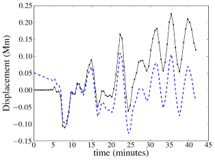
Figure 6: Solid black line: displacement of the center of mass at the apex, in the y-direction. Dashed blue line, the oscillating signal after the mean displacement is subtracted.

In the same figure, we see that there is an additional band of frequencies near $f=2$ mHz in the normalized power spectral density plot. From the equation of the Strouhal number, and assuming that its values are $St\sim 0.2$, this frequency can be obtained for velocities of the order of $20\times 10^{4}$ m s^-1. As we can see from the velocity profile at the apex (Figure 7; also hinted from the velocity field in Figure 4), the velocity field in front of the loop drops to values around $20-25$ km s^-1. This could potentially explain the peak near $2$ mHz, as the frequency imposed by the flow. Additionally, the fact that the loop cross-section changes over time will inevitably affect the frequency imposed by vortex shedding, explaining the width of the frequency band around $2$ mHz. Also, it is possible that the value of the Strouhal number in 3D environments in the presence of magnetic field needs is different from the one calculated in Gruszecki et al. (2010) for the 2D case. A full 3D parameter study was outside the scope of this work, and therefore not addressed here. However, the aforementioned frequency band near $2$ mHz seems to be dictated by the Strouhal number of the flow, as shown in the following paragraph.

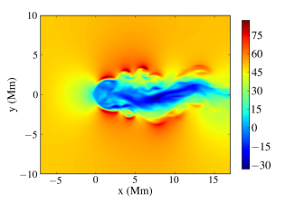
Figure 7: Profile of the $v_{x}$ ($\times 10^{3}$ m s^-1) velocity at the apex, for part off our datacube depicting the loop at $t=1012$ s.

As the final step, we want to test whether driving an oscillation via vortex shedding is a self-oscillating process. For that, we have considered a secondary setup, identical to the one described in section 2, but with internal and external magnetic field values of $B_{zi}=45.6$ G and $B_{ze}=45.64$ G, respectively, doubling the Alfvén speed and halving the period of the fundamental kink oscillation. In this new setup, we chose to drive the background flow for the whole duration of the simulation $\Delta t=2536$ s, because the stronger magnetic field makes the loop “stiffer,” delaying the start of the oscillation. This new loop has a fundamental kink mode frequency of $\sim 7.9$ mHz, represented by a strong peak in the normalized power spectral density plot for its nondetrended oscillating displacement, seen in Figure 8. This peak is different from the one dictated by the Strouhal number of the flow, which has the same velocity as before. The strong signal at near-zero frequencies due to the loop mean displacement is also shown here, as was in the case in the nondetrended signal from Figure 5. A wide frequency band between $2$ and $4$ mHz is also visible in this setup, showing that it is indeed dictated by the Strouhal number of the flow, as was previously mentioned, rather than the loop. The fact that the loop eigenfrequency is prominent, while the flow velocity is the same as before, shows that the loop is amplifying or imposing its own preferred frequency. Additionally, since the driving comes from an initially uniform and steady background flow, this process fits the definition of a self-oscillation (Jenkins, 2013).

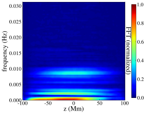
Figure 8: Plot of the normalized power spectral density for the oscillation of the loop with internal and external magnetic field values of $B_{zi}=45.6$ G and $B_{ze}=45.64$ G (secondary setup).

4 Summary and Conclusion

Although the idea that vortex shedding can excite standing waves in coronal loops has been proposed in Nakariakov et al. (2009), this mechanism had not been properly explored in a full 3D MHD model. The phenomenon of Alfvénic vortex shedding has already been studied for a bluff body in 2D by Gruszecki et al. (2010). However, a coronal loop will interact differently with a background flow than a fixed and rigid bluff body, and thus a study in 3D was essential. In the current work we see that a nonrigid loop will be deformed when interacting with a background flow. In addition, we see for the first time in a 3D simulation that the vortex shedding will eventually force the loop into an oscillation in the direction perpendicular to the flow, as was first proposed in Nakariakov et al. (2009).

The long duration of the vortex-shedding driving and the oscillation amplitudes comparable to the those found in Anfinogentov et al. (2015) make this mechanism a good candidate for generating decay-less oscillations. However, once the background flow is no longer present, the oscillations would start decaying. Thus, also decaying oscillations could potentially be generated via vortex shedding for short-lived background flows.

The mechanism of vortex shedding induced oscillations seems to fall into the self-oscillation processes. These, as was described in Jenkins (2013), are processes that can turn a nonperiodic driving (like a background steady flow) into a periodic signal (like a loop oscillation). Although vortex shedding has a preferred periodicity, as described by the flow Strouhal number (Gruszecki et al., 2010), the spectral densities of two different loops have clearly shown strong peaks around the corresponding frequencies of their fundamental standing kink-modes and not near the peak dictated by the Strouhal number. This shows that the oscillating loop imposes its own frequency, which is a characteristic of self-oscillations. Future studies could also help identify some of the additional frequencies and harmonics observed, which could be important for coronal seismology.

Despite its successes though, our very simple model still only provides a proof-of-concept for sustaining decay-less oscillations through the vortex shedding, and additional studies are necessary. Although the results of Gruszecki et al. (2010) for the Strouhal number seem to match the hydrodynamical case, a full parameter study in 3D MHD should be performed, as this was outside the scope of the current study. In order to compare with observations, gravitationally stratified loops and realistic flow profiles should be considered. Changing the flow speed would change the location of frequency peak dictated by the Strouhal number, but it could also have catastrophic effects on the loop cross-section, should the flow be too strong or the loop not “stiff” enough (i.e. having a weaker magnetic field). In addition, the loop characteristics are expected to affect the resulting oscillation amplitudes, and thus the strength of the different frequency peaks.

References

- Afanasyev et al. (2019) Afanasyev, A., Karampelas, K., & Van Doorsselaere, T. 2019, ApJ, 876, 100, doi: 10.3847/1538-4357/ab1848
- Afanasyev et al. (2020) Afanasyev, A. N., Van Doorsselaere, T., & Nakariakov, V. M. 2020, A&A, 633, L8, doi: 10.1051/0004-6361/201937187
- Anfinogentov et al. (2013) Anfinogentov, S., Nisticò, G., & Nakariakov, V. M. 2013, A&A, 560, A107, doi: 10.1051/0004-6361/201322094
- Anfinogentov & Nakariakov (2019) Anfinogentov, S. A., & Nakariakov, V. M. 2019, ApJ, 884, L40, doi: 10.3847/2041-8213/ab4792
- Anfinogentov et al. (2015) Anfinogentov, S. A., Nakariakov, V. M., & Nisticò, G. 2015, A&A, 583, A136, doi: 10.1051/0004-6361/201526195
- Antolin et al. (2016) Antolin, P., Moortel, I. D., Doorsselaere, T. V., & Yokoyama, T. 2016, The Astrophysical Journal Letters, 830, L22. http://stacks.iop.org/2041-8205/830/i=2/a=L22
- Antolin et al. (2014) Antolin, P., Yokoyama, T., & Van Doorsselaere, T. 2014, The Astrophysical Journal Letters, 787, L22
- Aschwanden et al. (1999) Aschwanden, M. J., Fletcher, L., Schrijver, C. J., & Alexander, D. 1999, ApJ, 520, 880, doi: 10.1086/307502
- Duckenfield et al. (2018) Duckenfield, T., Anfinogentov, S. A., Pascoe, D. J., & Nakariakov, V. M. 2018, ApJ, 854, L5, doi: 10.3847/2041-8213/aaaaeb
- Edwin & Roberts (1983) Edwin, P. M., & Roberts, B. 1983, Sol. Phys., 88, 179, doi: 10.1007/BF00196186
- Froment et al. (2017) Froment, C., Auchère, F., Aulanier, G., et al. 2017, ApJ, 835, 272, doi: 10.3847/1538-4357/835/2/272
- Goossens et al. (2011) Goossens, M., Erdélyi, R., & Ruderman, M. S. 2011, Space science reviews, 158, 289
- Gruszecki et al. (2010) Gruszecki, M., Nakariakov, V. M., van Doorsselaere, T., & Arber, T. D. 2010, Phys. Rev. Lett., 105, 055004, doi: 10.1103/PhysRevLett.105.055004
- Guo et al. (2019) Guo, M., Van Doorsselaere, T., Karampelas, K., et al. 2019, ApJ, 870, 55, doi: 10.3847/1538-4357/aaf1d0
- Heyvaerts & Priest (1983) Heyvaerts, J., & Priest, E. R. 1983, A&A, 117, 220
- Hillier et al. (2019) Hillier, A., Barker, A., Arregui, I., & Latter, H. 2019, MNRAS, 482, 1143, doi: 10.1093/mnras/sty2742
- Ionson (1978) Ionson, J. A. 1978, ApJ, 226, 650, doi: 10.1086/156648
- Jenkins (2013) Jenkins, A. 2013, Phys. Rep., 525, 167, doi: 10.1016/j.physrep.2012.10.007
- Karampelas & Van Doorsselaere (2020) Karampelas, K., & Van Doorsselaere, T. 2020, ApJ, 897, L35, doi: 10.3847/2041-8213/ab9f38
- Karampelas et al. (2017) Karampelas, K., Van Doorsselaere, T., & Antolin, P. 2017, A&A, 604, A130, doi: 10.1051/0004-6361/201730598
- Karampelas et al. (2019) Karampelas, K., Van Doorsselaere, T., Pascoe, J. D., Guo, M., & Antolin, P. 2019, Frontiers in Astronomy and Space Sciences, 6, 38, doi: 10.3389/fspas.2019.00038
- Magyar et al. (2015) Magyar, N., Van Doorsselaere, T., & Marcu, A. 2015, A&A, 582, A117, doi: 10.1051/0004-6361/201526287
- McIntosh et al. (2011) McIntosh, S. W., de Pontieu, B., Carlsson, M., et al. 2011, Nature, 475, 477, doi: 10.1038/nature10235
- Mignone et al. (2012) Mignone, A., Zanni, C., Tzeferacos, P., et al. 2012, ApJS, 198, 7, doi: 10.1088/0067-0049/198/1/7
- Nakariakov et al. (2016) Nakariakov, V. M., Anfinogentov, S. A., Nisticò, G., & Lee, D.-H. 2016, A&A, 591, L5, doi: 10.1051/0004-6361/201628850
- Nakariakov et al. (2009) Nakariakov, V. M., Aschwanden, M. J., & van Doorsselaere, T. 2009, A&A, 502, 661, doi: 10.1051/0004-6361/200810847
- Nakariakov & Ofman (2001) Nakariakov, V. M., & Ofman, L. 2001, A&A, 372, L53, doi: 10.1051/0004-6361:20010607
- Nakariakov et al. (1999) Nakariakov, V. M., Ofman, L., Deluca, E. E., Roberts, B., & Davila, J. M. 1999, Science, 285, 862, doi: 10.1126/science.285.5429.862
- Nakariakov & Verwichte (2005) Nakariakov, V. M., & Verwichte, E. 2005, Living Reviews in Solar Physics, 2, 3, doi: 10.12942/lrsp-2005-3
- Nechaeva et al. (2019) Nechaeva, A., Zimovets, I. V., Nakariakov, V. M., & Goddard, C. R. 2019, ApJS, 241, 31, doi: 10.3847/1538-4365/ab0e86
- Nisticò et al. (2013) Nisticò, G., Nakariakov, V. M., & Verwichte, E. 2013, A&A, 552, A57, doi: 10.1051/0004-6361/201220676
- Nisticò et al. (2018) Nisticò, G., Vladimirov, V., Nakariakov, V. M., Battams, K., & Bothmer, V. 2018, A&A, 615, A143, doi: 10.1051/0004-6361/201732474
- Samanta et al. (2019) Samanta, T., Tian, H., & Nakariakov, V. M. 2019, Phys. Rev. Lett., 123, 035102, doi: 10.1103/PhysRevLett.123.035102
- Shi et al. (2021) Shi, M., Van Doorsselaere, T., Guo, M., et al. 2021, arXiv e-prints, arXiv:2101.01019. https://arxiv.org/abs/2101.01019
- Terradas et al. (2008) Terradas, J., Andries, J., Goossens, M., et al. 2008, ApJ, 687, L115, doi: 10.1086/593203
- Tian et al. (2012) Tian, H., McIntosh, S. W., Wang, T., et al. 2012, ApJ, 759, 144, doi: 10.1088/0004-637X/759/2/144
- Tomczyk et al. (2007) Tomczyk, S., McIntosh, S. W., Keil, S. L., et al. 2007, Science, 317, 1192, doi: 10.1126/science.1143304
- Van Doorsselaere et al. (2008) Van Doorsselaere, T., Nakariakov, V. M., & Verwichte, E. 2008, The Astrophysical Journal Letters, 676, L73
- Van Doorsselaere et al. (2020) Van Doorsselaere, T., Srivastava, A. K., Antolin, P., et al. 2020, arXiv e-prints, arXiv:2012.01371. https://arxiv.org/abs/2012.01371
- Wang et al. (2012) Wang, T., Ofman, L., Davila, J. M., & Su, Y. 2012, ApJ, 751, L27, doi: 10.1088/2041-8205/751/2/L27
- Yang et al. (2020) Yang, Z., Bethge, C., Tian, H., et al. 2020, Science, 369, 694, doi: 10.1126/science.abb4462
- Zajtsev & Stepanov (1975) Zajtsev, V. V., & Stepanov, A. V. 1975, Issledovaniia Geomagnetizmu Aeronomii i Fizike Solntsa, 37, 3
- Zimovets & Nakariakov (2015) Zimovets, I. V., & Nakariakov, V. M. 2015, A&A, 577, A4, doi: 10.1051/0004-6361/201424960