Symbolic Models for Infinite Networks of Control Systems: A Compositional Approach

Abstract.

This paper presents a compositional framework for the construction of symbolic models for a network composed of a countably infinite number of finite-dimensional discrete-time control subsystems. We refer to such a network as infinite network. The proposed approach is based on the notion of alternating simulation functions. This notion relates a concrete network to its symbolic model with guaranteed mismatch bounds between their output behaviors. We propose a compositional approach to construct a symbolic model for an infinite network, together with an alternating simulation function, by composing symbolic models and alternating simulation functions constructed for subsystems. Assuming that each subsystem is incrementally input-to-state stable and under some small-gain type conditions, we present an algorithm for orderly constructing local symbolic models with properly designed quantization parameters. In this way, the proposed compositional approach can provide us a guideline for constructing an overall symbolic model with any desired approximation accuracy. A compositional controller synthesis scheme is also provided to enforce safety properties on the infinite network in a decentralized fashion. The effectiveness of our result is illustrated through a road traffic network consisting of infinitely many road cells.

1. Introduction

Over the past few decades, large-scale interconnected systems have emerged in a wide range of safety-critical applications, such as traffic networks, smart manufacturing, and power networks. In such applications, the number of agents can be extremely large, possibly unknown, or even vary over time as agents plug in and out. Unless rigorously addressed, such scalability issues may dramatically degrade system performance [1, 2]. It is a reasonable strategy to over-approximate the original network with the limit case in size, in the sense that we introduce a network having infinitely many subsystems which includes the original network. We call this over-approximated network an infinite network [3, 4, 5]. Note that as a special class of infinite-dimensional systems, infinite networks require a rigorous treatment with careful choice of the infinite-dimensional state space of the overall network. It is widely acknowledged that infinite networks capture the essence of the original network, in the sense that functionality indices, e.g. transient and steady-states behaviors, of an infinite network are preserved for its corresponding original finite network; see, e.g., [1, 6]. In that way, one can eventually develop scale-free (i.e., independent of the system size) approaches for the analysis and control of a finite, but arbitrarily large network [7, 8, 6, 9].

This paper is mainly concerned with symbolic controller synthesis for infinite networks. In the past few years, symbolic model (a.k.a. finite abstraction) based techniques have been widely developed to assist in the analysis/synthesis of controllers enforcing complex specifications which are difficult to handle using classical control design methods [10, 11, 12]. Specifically, symbolic models are abstract descriptions of original dynamics. In this regard, one can first build up a symbolic model of the original complex system, then perform analysis or synthesis over the symbolic model in an automated fashion (employing automata-theoretic techniques developed in the computer science literatures [13]), and finally translate the results back to the original system with correctness guarantees. A major challenge in the construction of symbolic models for large-scale networks is the curse of dimensionality, i.e., the computational complexity of constructing symbolic models grows exponentially with the dimension of the system. In this paper, we aim at proposing a scale-free approach to alleviate the computational complexity in the construction of symbolic models for arbitrarily large-scale (potentially infinite) networks. A promising solution is to apply a divide and conquer scheme, namely, compositional approach. In this framework, the overall network is decomposed into a set of finite lower-dimensional subsystems, for which symbolic models can be individually constructed in a computationally efficient way. Then, a symbolic model for the overall network can be obtained by aggregating those of the subsystems. Various compositional approaches have been explored in the past decade for the construction of symbolic models; see, e.g., [14, 15, 16, 17, 18, 19, 20]. The results in [14, 15, 17, 18] leverage small-gain type conditions to compositionally construct so-called complete abstractions for a finite network. The results presented in [16] introduce a different compositionality framework based on dissipativity theory. The recent results in [19, 20] provide compositional construction of so-called sound abstractions for a large-scale system without imposing compositionality conditions. Although promising, all of the above-mentioned compositional approaches are typically tailored to a network composed of a finite number of subsystems and do not address the scalability issues discussed earlier.

In this paper, we develop a compositional approach for the construction of symbolic models for infinite networks. We first introduce a notion of so-called alternating simulation functions used to relate an infinite network to its symbolic model with bounded mismatch between the output behaviors of them. Then, we provide a compositionality result showing that an overall symbolic model can be obtained by composing those of subsystems. Particularly, for a network composed of infinitely many incrementally input-to-state stable control subsystems, we leverage a recently presented small-gain theorem [4] and present an algorithm to design quantization parameters for the construction of local symbolic models and local simulation functions in a systematic way. In particular, we give a top-down, still compositional, algorithm computing local quantization parameters with the guarantee of obtaining an overall symbolic model with any desired precision. This differentiates our approach from existing ones as discussed in the sequel (cf. Related Works below). Moreover, we present a decentralized controller synthesis approach for an infinite network that needs to meet safety specifications. It is shown that by composing local safety controllers which are synthesized for subsystems individually, the resulting overall controller enforces the safety specification on the overall infinite network with a formal guarantee. Finally, the effectiveness of our proposed framework is verified through a road traffic network containing infinitely many road cells.

Related Works. There have been several attempts on the construction of symbolic models for infinite-dimensional systems [21, 22]. The result in [21] deals with continuous time-delay systems, for which symbolic models are obtained by projecting the infinite-dimensional functional state-space on a finite-dimensional subspace. The result in [22] provides a state-space discretization-free approach which can be applied to possibly infinite-dimensional incrementally stable control systems. Although the results in [21, 22] are developed for (time-delay) infinite-dimensional systems, either state or input sets can be infinite dimensional. Here, we allow both state and input sets to be in infinite-dimensional space. Moreover, the results in [21, 22] take a monolithic view of the systems while constructing symbolic models. Therefore, in the case of potential application to an infinite network, the results in [21, 22] lose the network structure, and hence, they cannot be used for distributed control purposes. Here, we propose a compositional approach for the construction of symbolic models for infinite networks, such that the network structures are preserved. A preliminary investigation of our proposed method appeared in [9]. Our results here improve and extend those in [9] in three directions: 1) In this paper, we provide a detailed and mature description of the results presented in [9], including all proofs. 2) Here, we provide a top-down compositional framework: under certain small-gain type conditions, an algorithm is provided as a guideline to orderly design local quantization parameters with the guarantee of obtaining an overall symbolic model with any desired precision. Whereas [9] presents a bottom-top design approach, in the sense that one needs to first design local quantization parameters for subsystems and then use them to compute the overall approximation error. 3) In comparison with the proposed results in [9], due to the less conservatism in the definitions of alternating simulation functions in our work (cf. Definitions 3 and 5), our compositional approach can potentially provide symbolic models for infinite networks with much smaller approximation errors (cf. case study in Section 5).

2. Preliminaries

Notation: We denote by $\mathbb{R}$, $\mathbb{N}_{0}$, and $\mathbb{N}$ the sets of real numbers, non-negative integers, and positive integers, respectively. We denote the closed, open, and half-open intervals in $\mathbb{R}$ by $[a,b]$, $(a,b)$, $[a,b)$, and $(a,b]$, respectively. For $a,b\in\mathbb{N}_{0}$ and $a\leq b$, we use $[a;b]$, $(a;b)$, $[a;b)$, and $(a;b]$ to denote the corresponding intervals in $\mathbb{N}_{0}$. Given any $\nu=(\nu_{1},\cdots,\nu_{n})\in\mathbb{R}^{n}$, we define by $|\nu|=\max_{1\leq i\leq n}|\nu_{i}|$ the infinity norm of $\nu$. We denote by $\text{card}(\cdot)$ the cardinality of a given set and by $\varnothing$ the empty set. For any set $S\subseteq\mathbb{R}^{n}$ of the form of finite union of boxes, e.g., $S=\bigcup_{j=1}^{M}S_{j}$ for some finite number $M\in\mathbb{N}$, where $S_{j}=\prod_{i=1}^{n}[c_{i}^{j},d_{i}^{j}]\subseteq\mathbb{R}^{n}$ with $c^{j}_{i}<d^{j}_{i}$, we define $\emph{span}(S)=\min_{j=1,\ldots,M}\eta_{S_{j}}$ and $\eta_{S_{j}}=\min\{|d_{1}^{j}-c_{1}^{j}|,\ldots,|d_{n}^{j}-c_{n}^{j}|\}$. Moreover, for a set in the form of $X=\prod_{i=1}^{N}X_{i}$, where $X_{i}\subseteq\mathbb{R}^{n_{i}}$, $\forall i\in[1;N]$, are of the form of finite union of boxes, and any positive (component-wise) vector $\phi=[\phi_{1};\dots;\phi_{N}]$ with $\phi_{i}\leq\emph{span}(X_{i})$, $\forall i\in[1;N]$, we define $[X]_{\phi}=\prod_{i=1}^{N}[X_{i}]_{\phi_{i}}$, where $[X_{i}]_{\phi_{i}}=[\mathbb{R}^{n_{i}}]_{\phi_{i}}\cap{X_{i}}$ and $[\mathbb{R}^{n_{i}}]_{\phi_{i}}=\{a\in\mathbb{R}^{n_{i}}\mid a_{j}=k_{j}\phi_{i},k_{j}\in\mathbb{Z},j=1,\ldots,n_{i}\}$. Note that if $\phi=[\eta;\dots;\eta]$, where $0\leq\eta\leq\emph{span}(S)$, we simply use notation $[S]_{\eta}$ rather than $[S]_{\phi}$. Note that $[S]_{\eta}\neq\emptyset$ for any $0\leq\eta\leq\emph{span}(S)$. We use the notations $\mathcal{K}$ and $\mathcal{K}_{\infty}$ to denote different classes of comparison functions, as follows: $\mathcal{K}=\{\alpha:\mathbb{R}_{\geq 0}\rightarrow\mathbb{R}_{\geq 0}|$ $\alpha$ is continuous, strictly increasing, and $\alpha(0)=0\}$; $\mathcal{K}_{\infty}=\{\alpha\in\mathcal{K}|$ $\lim\limits_{r\rightarrow\infty}\alpha(r)=\infty\}$. For $\alpha,\gamma\!\in\!\mathcal{K}_{\infty}$ we write $\alpha\!\leq\!\gamma$ if $\alpha(r)\!\leq\!\gamma(r)$, and, with a slight abuse of the notation, $\alpha\!=\!c$ if $\alpha(r)\!=\!cr$ for all $c,r\!\geq\!0$. Finally, we denote by $\mathrm{id}$ the identity function over $\mathbb{R}_{\geq 0}$, i.e., $\mathrm{id}(r)=r$ for all $r\in\mathbb{R}_{\geq 0}$.

2.1. Infinite networks

In this paper, we study the interconnection of a countably infinite number of discrete-time control subsystems. Using $\mathbb{N}$ as the index set, the $i$-th subsystem is denoted by a tuple $\Sigma{{}_{i}}=(X{{}_{i}},U{{}_{i}},W{{}_{i}},f{{}_{i}},Y{{}_{i}},h{{}_{i}})$, where $X{{}_{i}}\subseteq\mathbb{R}^{n_{i}}$, $U{{}_{i}}\subseteq\mathbb{R}^{m_{i}}$, $W{{}_{i}}\subseteq\mathbb{R}^{p_{i}}$, $Y{{}_{i}}\subseteq\mathbb{R}^{q_{i}}$, are the state, external input, internal input, and output set, respectively. The set valued map $f{{}_{i}}:X{{}_{i}}\times U{{}_{i}}\times W{{}_{i}}\rightrightarrows X{{}_{i}}$ is the state transition function and $h{{}_{i}}:X{{}_{i}}\rightarrow Y{{}_{i}}$ is the output map. The discrete-time control subsystem $\Sigma{{}_{i}}$ is described by difference inclusions of the form

$$\Sigma_{i}:\left\{\begin{array}[]{rl}{\mathbf{x}}{{}_{i}}(k+1)\in&f{{}_{i}}(\mathbf{x}{{}_{i}}(k),\nu{{}_{i}}(k),\omega{{}_{i}}(k)),\\ \mathbf{y}{{}_{i}}(k)=&h{{}_{i}}(\mathbf{x}{{}_{i}}(k)),\end{array}\right.$$ (3)

where $\mathbf{x}_{i}:\mathbb{N}_{0}\rightarrow X_{i}$, $\mathbf{y}_{i}:\mathbb{N}_{0}\rightarrow Y_{i}$, $\nu_{i}:\mathbb{N}_{0}\rightarrow U_{i}$, and $\omega_{i}:\mathbb{N}_{0}\rightarrow W_{i}$ are the state, output, external input, and internal input signals, respectively. System $\Sigma_{i}$ is called deterministic if $\text{card}(f_{i}(x_{i},u_{i},w_{i}))\leq 1$, $\forall x_{i}\in X_{i},\forall u_{i}\in U_{i},\forall w_{i}\in W_{i}$, and non-deterministic otherwise. System $\Sigma_{i}$ is called discrete if $X_{i},U_{i},W_{i}$ are finite sets, and continuous otherwise.

Throughout the paper, we assume that each subsystem $\Sigma_{i}$ is affected by finitely many neighbors. For each $i\in\mathbb{N}$, the set of in-neighbors of $\Sigma_{i}$ is denoted by $\mathcal{N}_{i}\subset\mathbb{N}\setminus\{i\}$, i.e. the set of subsystems $\Sigma_{j}$, $j\in\mathcal{N}_{i}$, directly influencing $\Sigma_{i}$. On the other hand, the set of out-neighbors of $\Sigma_{i}$, denoted by $\mathcal{M}_{i}\subset\mathbb{N}\setminus\{i\}$, is the set of $\Sigma_{j}$, $j\in\mathcal{M}_{i}$, directly affected by $\Sigma_{i}$. Sets $\mathcal{N}_{i}$ and $\mathcal{M}_{i}$ are finite, though not necessarily uniformly. Formally, the input-output structure of each subsystem $\Sigma_{i}$, $i\in\mathbb{N}$, is given by

$$w_{i} =(w_{ij})_{j\in\mathcal{N}_{i}}\in W_{i}:=\prod_{j\in{\mathcal{N}_{i}}}W_{ij},$$ (4)

$$y_{i} =(y_{ij})_{j\in(i\cup{\mathcal{M}_{i}})}\in Y_{i}:=\prod_{j\in(i\cup{\mathcal{M}_{i}})}\!\!Y_{ij},$$ (5)

$$h_{i}(x_{i}) =(h_{ij}(x_{i}))_{j\in(i\cup{\mathcal{M}_{i}})},$$ (6)

with $w_{ij}\in W_{ij}$, $y_{ij}=h_{ij}(x_{i})\in Y_{ij}$. The outputs $y_{ii}$ are considered as external ones, whereas $y_{ij}$, $j\in\mathcal{M}_{i}$, are interpreted as internal ones which are used to construct an interconnection of subsystems.

In the sequel, we denote by $\ell^{\infty}$ the Banach space of all uniformly bounded sequences $s=(s_{i})_{i\in\mathbb{N}}\in\ell^{\infty}$, where $s_{i}\in\mathbb{R}^{n_{i}}$ denotes the $i$-th position of a sequence $s\in\ell^{\infty}$. The $\ell^{\infty}$ space is defined as

$$\ell^{\infty}(\mathbb{N},(n_{i})):=\left\{s=(s_{i})_{i\in\mathbb{N}}:s_{i}\in\mathbb{R}^{n_{i}},\sup_{i\in\mathbb{N}}|s_{i}|<\infty\right\},$$ (7)

endowed with the norm $\|s\|:=\sup_{i\in\mathbb{N}}|s_{i}|$. Moreover, we use $\ell^{\infty}_{+}$ to denote the positive cone in $\ell^{\infty}$ consisting of all vectors $s\in\ell^{\infty}$ with $s_{i}\geq 0,i\in\mathbb{N}$. We denote by $\textup{int}(\ell^{\infty}_{+})$ the interior of $\ell^{\infty}_{+}$.

Now, we are ready to provide a formal definition of the infinite network.

Definition 1.

Consider subsystems $\Sigma_{i}=(X_{i},U_{i},W_{i},f_{i},Y_{i},h_{i}),~{}i\in\mathbb{N},$ with input-output structure given by (4) to (6). An infinite network is formally a tuple $\Sigma=(X,U,f,Y,h)$, where $X=\{x=(x_{i})_{i\in\mathbb{N}}:x_{i}\in X_{i}\}$, $U=\{u=(u_{i})_{i\in\mathbb{N}}:u_{i}\in U_{i}\}$, $f(x,u)=\{(x^{+}_{i})_{i\in\mathbb{N}}|x_{i}^{+}\in f_{i}(x_{i},u_{i},w_{i})\}$, $Y=\prod_{i\in\mathbb{N}}Y_{ii}$, $h(x)=(h_{ii}(x_{i}))_{i\in\mathbb{N}}$. A concrete infinite network $\Sigma=(X,U,f,Y,h)$, denoted by $\Sigma=\mathcal{I}(\Sigma_{i})_{i\in\mathbb{N}}$, consists of infinitely many continuous subsystems $\Sigma_{i}$, with the interconnection variables constrained by

$$\forall i\in\mathbb{N},\forall j\in\mathcal{N}_{i},w_{ij}=y_{ji},Y_{ji}\subseteq W_{ij}.$$ (8)

An abstract infinite network $\hat{\Sigma}=(\hat{X},\hat{U},\hat{f},\hat{Y},\hat{h})$, denoted by $\hat{\Sigma}=\mathcal{I}(\hat{\Sigma}_{i})_{i\in\mathbb{N}}$, is composed of infinitely many discrete subsystems, with the interconnection variables constrained by

$$\forall i\in\mathbb{N},\forall j\in\mathcal{N}_{i},|\hat{y}_{ji}-\hat{w}_{ij}|\leq\phi_{ij},[\hat{{Y}}_{ji}]_{\phi_{ij}}\subseteq\hat{{W}}_{ij},$$ (9)

where $\phi_{ij}\in\mathbb{R}_{\geq 0}$ is an internal input quantization parameter designed later (cf. Definition 9).

Throughout the paper, we assume that $f(x,u)\in X$ for all $(x,u)\in X\times U$, which ensures that the infinite network is well-posed.

Remark 2.

Note that in Definition 1, the interconnection constraint in (8) for the concrete network is different from (9) for the abstract network. For a network of symbolic models, we allow for possibly different granularities of finite internal input sets $\hat{W}_{ij}$ and output sets $\hat{Y}_{ji}$, and introduce parameters $\phi_{ij}$ in (9) for having a well-posed interconnection. The values of $\phi_{ij}$ will be designed later in Definition 9 while constructing local symbolic models of subsystems. $\diamond$

2.2. Alternating simulation functions

Here, we provide a notion of alternating simulation functions which quantitatively relate two infinite networks.

Definition 3.

Consider infinite networks $\Sigma\!=(X,U,f,Y,h)$ and $\hat{\Sigma}\!=(\hat{{X}},\hat{{U}},\hat{f},$ $\hat{{Y}},\hat{h})$, where $\hat{{Y}}\subseteq{{Y}}$. For $\varpi\in\mathbb{R}_{\geq 0}$, a function $\tilde{V}:X\times\hat{{X}}\rightarrow\mathbb{R}_{\geq 0}$ is called an $\varpi$-approximate alternating simulation function ($\varpi$-ASF) from $\hat{\Sigma}$ to $\Sigma$, if there exists a function $\alpha\in\mathcal{K_{\infty}}$ such that

1. For all $x\in X$, $\hat{x}\in\hat{X}$, one has

   $$\alpha(\|h(x)-\hat{h}(\hat{x})\|)\leq\tilde{V}(x,\hat{x});$$ (10)

2. For all $x\in X$ and $\hat{x}\in\hat{X}$ with $\tilde{V}(x,\hat{x})\leq\varpi$, for all $\hat{u}\in\hat{{U}}$, there exists $u\in U$ such that for all $x^{+}\in f(x,u)$, there exists $\hat{x}^{+}\in\hat{f}(\hat{x},\hat{u})$ so that

   $$\tilde{V}(x^{+},\hat{x}^{+})\leq\varpi.$$ (11)

If there exists an alternating simulation function from $\hat{\Sigma}$ to $\Sigma$, $\hat{\Sigma}$ is called an abstraction of $\Sigma$. Additionally, if $\hat{\Sigma}$ is discrete ($\hat{X}$ and $\hat{U}$ are finite sets), $\hat{\Sigma}$ is called a symbolic model (or finite abstraction) of the concrete network $\Sigma$.

Remark 4.

Definition 3 implies that the relation $R\subseteq{X}\times\hat{{X}}$ defined by $R=\left\{(x,\hat{x})\in{X}\times\hat{{X}}|\tilde{V}(x,\hat{x})\leq\varpi\right\}$ is an $\hat{\varepsilon}$-approximate alternating simulation relation, defined in [11], from $\hat{\Sigma}$ to $\Sigma$ with $\hat{\varepsilon}=\alpha^{-1}(\varpi)$. As shown in [11], the existence of an $\varpi$-ASF enables us to design a controller for the abstract network $\hat{\Sigma}$, and refine the controller back to the concrete network $\Sigma$. $\diamond$

3. Compositional Construction of Symbolic Models

In this section, we provide a method for compositional construction of an alternating simulation function between two infinite networks $\Sigma=\mathcal{I}(\Sigma_{i})_{i\in\mathbb{N}}$ and $\hat{\Sigma}=\mathcal{I}(\hat{\Sigma}_{i})_{i\in\mathbb{N}}$. Here, we assume that each pair of subsystems $\Sigma_{i}=(X_{i},W_{i},U_{i},f_{i},Y_{i},h_{i})$ and $\hat{\Sigma}_{i}\!=(\hat{{X}}_{i},\hat{{W}}_{i},\hat{{U}}_{i},\hat{f}_{i},\hat{{Y}}_{i},\hat{h}_{i})$ admit a local alternating simulation function as defined next.

Definition 5.

Consider subsystems $\Sigma_{i}=(X_{i},U_{i},W_{i},f_{i},Y_{i},h_{i})$ and $\hat{\Sigma}_{i}=(\hat{{X}}_{i},$ $\hat{{U}}_{i},\hat{{W}}_{i},\hat{f}_{i},\hat{{Y}}_{i},\hat{h}_{i})$ where $\hat{{W}}_{i}\subseteq{W_{i}}$ and $\hat{{Y}}_{i}\subseteq{Y_{i}}$. Given $\varpi_{i}\in\mathbb{R}_{\geq 0}$, a function $V_{i}:X_{i}\times\hat{X}_{i}\rightarrow\mathbb{R}_{\geq 0}$ is called a local $\varpi_{i}$-ASF from $\hat{\Sigma}_{i}$ to $\Sigma_{i}$, if there exist a constant $\vartheta_{i}\in\mathbb{R}_{\geq 0}$, and functions $\underline{\alpha}_{i},\overline{\alpha}_{i}\in\mathcal{K_{\infty}}$ such that

1. For all $x_{i}\in X_{i}$, all $\hat{x}_{i}\in\hat{X}_{i}$, one has

   $$\underline{\alpha}_{i}(|h_{i}(x_{i})-\hat{h}_{i}(\hat{x}_{i})|)\leq V_{i}(x_{i},\hat{x}_{i})\leq{\overline{\alpha}}_{i}(|x_{i}-\hat{x}_{i}|).$$ (12)

2. For all $x_{i}\in X_{i}$, all $\hat{x}_{i}\in\hat{X}_{i}$ with $V_{i}(x_{i},\hat{x}_{i})\leq\varpi_{i}$, for all $w_{i}\in W_{i}$, all $\hat{w}_{i}\in\hat{{W}}_{i}$ with $|w_{i}-\hat{w}_{i}|\leq\vartheta_{i}$, for all $\hat{u}_{i}\in\hat{{U}}_{i}$, there exists $u_{i}\in U_{i}$ such that for all $x_{i}^{+}\in f_{i}(x_{i},u_{i},w_{i})$, there exists $\hat{x}_{i}^{+}\in\hat{f}_{i}(\hat{x}_{i},\hat{u}_{i},\hat{w}_{i})$ so that

   $$V_{i}(x_{i}^{+},\hat{x}_{i}^{+})\leq\varpi_{i}.$$ (13)

If there exists a local alternating simulation function from $\hat{\Sigma}_{i}$ to $\Sigma_{i}$, $\hat{\Sigma}_{i}$ is called an abstraction of $\Sigma_{i}$. Additionally, if $\hat{\Sigma}_{i}$ is discrete ($\hat{X}_{i}$, $\hat{U}_{i}$, and $\hat{W}_{i}$ are finite sets), $\hat{\Sigma}_{i}$ is called a symbolic model (or finite abstraction) of the concrete subsystem $\Sigma_{i}$.

The next theorem provides a compositional approach for the construction of an alternating simulation function between two infinite networks using the above-defined local alternating simulation functions.

Theorem 6.

Consider an infinite network $\Sigma=\mathcal{I}(\Sigma_{i})_{i\in\mathbb{N}}$. Assume that each $\Sigma_{i}$ and its abstraction $\hat{\Sigma}_{i}$ admit a local $\varpi_{i}$-ASF $V_{i}$ equipped with functions $\underline{\alpha}_{i},\overline{\alpha}_{i}\in\mathcal{K_{\infty}}$ and constants $\varpi_{i},\vartheta_{i}\in\mathbb{R}_{\geq 0}$ as in Definition 5. Suppose that there exist $\underline{\alpha},\overline{\alpha}\in\mathcal{K}_{\infty}$, and constants $\underline{\varpi},\varpi\in\mathbb{R}_{\geq 0}$ such that for each $i\in\mathbb{N}$

$$\underline{\alpha}\leq\underline{\alpha}_{i}\leq\overline{\alpha}_{i}\leq\overline{\alpha},$$ (14)

$$\underline{\varpi}\leq{\varpi_{i}}\leq{\varpi}.$$ (15)

For each $i\in\mathbb{N}$ and $j\in\mathcal{N}_{i}$, let functions $\underline{\alpha}_{j}$, constants $\varpi_{j},\vartheta_{i}$, and constants $\phi_{ij}$ as in (9) satisfy the following inequality

$${\underline{\alpha}}^{-1}_{j}(\varpi_{j})+\phi_{ij}\leq\vartheta_{i}.$$ (16)

Then, function

$$\tilde{V} (x,\hat{x}):=\sup\limits_{i\in\mathbb{N}}\{\frac{{\varpi}}{\varpi_{i}}V_{i}(x_{i},\hat{x}_{i})\},$$ (17)

is well-defined and it is an $\varpi$-ASF from $\hat{\Sigma}=\mathcal{I}(\hat{\Sigma}_{i})_{i\in\mathbb{N}}$ to $\Sigma=\mathcal{I}(\Sigma_{i})_{i\in\mathbb{N}}$.

Proof.

First we show that function $\tilde{V}$ constructed as in (17) is well-defined. Note that for all $x\in X$ and for all $\hat{x}\in\hat{X}$ we have

$$\tilde{V}(x,\hat{x}) :=\sup\limits_{i\in\mathbb{N}}\{\frac{\varpi}{\varpi_{i}}V_{i}(x_{i},\hat{x}_{i})\}\stackrel{{\scriptstyle\eqref{localineq1}}}{{\leq}}\varpi\sup\limits_{i\in\mathbb{N}}\{\varpi^{-1}_{i}\overline{\alpha}_{i}(|x_{i}-\hat{x}_{i}|)\}$$

$$\leq\varpi\sup\limits_{i\in\mathbb{N}}\{\varpi^{-1}_{i}\overline{\alpha}_{i}(|x_{i}|+|\hat{x}_{i}|)\}\stackrel{{\scriptstyle\eqref{mainineq2}}}{{\leq}}\varpi\sup\limits_{i\in\mathbb{N}}\{\underline{\varpi}^{-1}\overline{\alpha}(|x_{i}|+|\hat{x}_{i}|)\}$$

$$\leq\frac{\varpi}{\underline{\varpi}}\overline{\alpha}\sup\limits_{i\in\mathbb{N}}\{|x_{i}|+|\hat{x}_{i}|\}\leq\frac{\varpi}{\underline{\varpi}}\overline{\alpha}(\sup\limits_{i\in\mathbb{N}}\{|x_{i}|\}+\sup\limits_{i\in\mathbb{N}}\{|\hat{x}_{i}|\})$$

$$\stackrel{{\scriptstyle\eqref{infnorm}}}{{\leq}}\frac{\varpi}{\underline{\varpi}}\overline{\alpha}(\|x\|+\|\hat{x}\|)<\infty.$$

Next, we show that there exists ${\alpha}\in\mathcal{K}_{\infty}$ such that condition (i) of Definition 3 holds. Consider any $x\in X$, $\hat{x}\in{\hat{X}}$, one gets

$$\|h(x)-\hat{h}(\hat{x})\| =\sup\limits_{i\in\mathbb{N}}\{|h_{ii}(x_{i})-\hat{h}_{ii}(\hat{x}_{i})|\}\stackrel{{\scriptstyle\eqref{outputfunction}}}{{\leq}}\sup\limits_{i\in\mathbb{N}}\{|h_{i}(x_{i})-\hat{h}_{i}(\hat{x}_{i})|\}$$

$$\stackrel{{\scriptstyle\eqref{localineq1}}}{{\leq}}\sup\limits_{i\in\mathbb{N}}\{\underline{\alpha}^{-1}_{i}(V_{i}(x_{i},\hat{x}_{i}))\}=\sup\limits_{i\in\mathbb{N}}\{\underline{\alpha}^{-1}_{i}(\varpi_{i}\varpi^{-1}_{i}V_{i}(x_{i},\hat{x}_{i}))\}$$

$$\stackrel{{\scriptstyle\eqref{mainineq1}\eqref{mainineq2}}}{{\leq}}\underline{\alpha}^{-1}\sup\limits_{i\in\mathbb{N}}\{\varpi\varpi^{-1}_{i}(V_{i}(x_{i},\hat{x}_{i}))\}\stackrel{{\scriptstyle\eqref{defVinit}}}{{=}}\underline{\alpha}^{-1}(\tilde{V}(x,\hat{x})).$$

Hence, condition (i) holds with $\alpha:=\underline{\alpha}$. Next, we show that condition (ii) of Definition 3 is satisfied. Let us consider any $x=(x_{i})_{i\in\mathbb{N}}\in X$ and $\hat{x}=(\hat{x}_{i})_{i\in\mathbb{N}}\in\hat{{X}}$ such that $\tilde{V}(x,\hat{x})\leq\varpi$. It can be seen that from the construction of $\tilde{V}$ in (17), we have $V_{i}(x_{i},\hat{x}_{i})\leq\varpi_{i}$, for each $i\in\mathbb{N}$. For each pair of subsystems $\Sigma_{i}$ and $\hat{\Sigma}_{i}$, the internal inputs satisfy the following inequality

$$|w_{i}-\hat{w}_{i}|= \max\limits_{j\in\mathcal{N}_{i}}\{|w_{ij}-\hat{w}_{ij}|\}\stackrel{{\scriptstyle\eqref{const}}}{{=}}\max\limits_{j\in\mathcal{N}_{i}}\{|y_{ji}-\hat{y}_{ji}+\hat{y}_{ji}-\hat{w}_{ij}|\}$$

$$\stackrel{{\scriptstyle\eqref{const1}}}{{\leq}} \max\limits_{j\in\mathcal{N}_{i}}\{|y_{ji}-\hat{y}_{ji}|+\phi_{ij}\}\leq\max\limits_{j\in\mathcal{N}_{i}}\{|h_{j}(x_{j})-\hat{h}_{j}(\hat{x}_{j})|+\phi_{ij}\}$$

$$\stackrel{{\scriptstyle\eqref{localineq1}}}{{\leq}} \max\limits_{j\in\mathcal{N}_{i}}\{{\underline{\alpha}}^{-1}_{j}V_{j}(x_{j},\hat{x}_{j})+\phi_{ij}\}\leq\max\limits_{j\in\mathcal{N}_{i}}\{{\underline{\alpha}}^{-1}_{j}(\varpi_{j})+\phi_{ij}\}.$$

Using (16), one has $|w_{i}-\hat{w}_{i}|\leq\vartheta_{i}$ for each $i\in\mathbb{N}$. Therefore, by Definition 5 for each pair of subsystems $\Sigma_{i}$ and $\hat{\Sigma}_{i}$, one has for any $\hat{u}_{i}\in\hat{U}_{i}$, there exists $u_{i}\in U_{i}$ such that for any $x_{i}^{+}\in f_{i}(x_{i},u_{i},w_{i})$, there exists $\hat{x}_{i}^{+}\in\hat{f}_{i}(\hat{x}_{i},\hat{u}_{i},\hat{w}_{i})$ such that $V_{i}(x_{i}^{+},\hat{x}_{i}^{+})\leq\varpi_{i}$. As a result, we get for any $\hat{u}=(\hat{u}_{i})_{i\in\mathbb{N}}\in\hat{{U}}$, there exists $u=(u_{i})_{i\in\mathbb{N}}\in U$, such that for any $x^{+}=(x_{i}^{+})_{i\in\mathbb{N}}\in f(x,u)$, there exists $\hat{x}^{+}=(\hat{x}_{i}^{+})_{i\in\mathbb{N}}\in\hat{f}(\hat{x},\hat{u})$ such that $\tilde{V}(x^{+},\hat{x}^{+})=\sup\limits_{i\in\mathbb{N}}\{\frac{\varpi}{\varpi_{i}}V_{i}(x_{i},\hat{x}_{i})\}\leq\varpi$. Therefore, condition (ii) of Definition 3 is satisfied with $\varpi=\sup\limits_{i\in\mathbb{N}}\varpi_{i}$. Therefore, we conclude that $\tilde{V}$ is an $\varpi$-ASF from $\hat{\Sigma}=\mathcal{I}(\hat{\Sigma}_{i})_{i\in\mathbb{N}}$ to $\Sigma=\mathcal{I}(\Sigma_{i})_{i\in\mathbb{N}}$. ∎

Remark 7.

Note that practically speaking, the computation of a symbolic model consisting of infinite subsystems requires an infinite memory usage, which prevents us from having a central entity to handle the construction of a symbolic model for the overall network. However, the proposed compositional framework is still needed to formally establish the alternating simulation relation between infinite networks in terms of preserving desired properties. On this basis, one can develop decentralized (or distributed) schemes to solve controller synthesis problems compositionally using symbolic models of subsystems. $\diamond$

Next we provide a method to construct local symbolic models together with corresponding local alternating simulation functions for the concrete subsystems under incremental stability-type conditions.

3.1. Construction of local symbolic models

In this subsection, we present a method to construct a symbolic model $\hat{\Sigma}_{i}$, together with the corresponding local alternating simulation function, for a given finite-dimensional deterministic subsystem $\Sigma_{i}$. Consider a subsystem $\Sigma_{i}=(X_{i},U_{i},W_{i},f_{i},Y_{i},h_{i})$ as in (3). Assume that there exists $\ell\in\mathcal{K}$ such that the output map $h_{i}$ satisfies $|h_{i}(x_{i})-h_{i}(x_{i}^{\prime})|\leq\ell(|x_{i}-x_{i}^{\prime}|)$ for all $x_{i},x_{i}^{\prime}\in X_{i}$. Additionally, let $\Sigma_{i}$ be incrementally input-to-state stable ($\delta$-ISS) [23] as defined next.

Definition 8.

System $\Sigma_{i}$ is incrementally input-to-state stable ($\delta$-ISS) if there exist a so-called $\delta$-ISS Lyapunov function $\mathcal{V}_{i}:X_{i}\times X_{i}\to\mathbb{R}_{\geq 0}$, and functions ${\underline{\psi}_{i}},{\overline{\psi}_{i}},\kappa_{i},\rho_{w_{i}},\rho_{u_{i}}\in\mathcal{K}_{\infty}$, with $\kappa_{i}<\mathrm{id}$ such that for all $x_{i},x^{\prime}_{i}\in X_{i}$, all $w_{i},w^{\prime}_{i}\in W_{i}$, and all $u_{i},u^{\prime}_{i}\in U_{i}$

$$\underline{\psi}_{i}(|x_{i}-x^{\prime}_{i}|)\leq \mathcal{V}_{i}(x_{i},x^{\prime}_{i})\leq\overline{\psi}_{i}(|x_{i}-x^{\prime}_{i}|),$$ (18)

$$\mathcal{V}_{i}(f_{i}(x_{i},u_{i},w_{i}),f_{i}(x^{\prime}_{i},u^{\prime}_{i},w^{\prime}_{i}))\leq \kappa_{i}(\mathcal{V}_{i}(x_{i},{x_{i}^{\prime}}))+\varrho_{w_{i}}(|w_{i}-w^{\prime}_{i}|)+\varrho_{u_{i}}(|u_{i}-u^{\prime}_{i}|).$$ (19)

We further assume that there exists $\hat{\gamma}_{i}\in\mathcal{K}_{\infty}$ such that for all $x_{i},x_{i}^{\prime},x_{i}^{\prime\prime}\in{X}_{i}$

$$\mathcal{V}_{i}(x_{i},x_{i}^{\prime})\leq\mathcal{V}_{i}(x_{i},x_{i}^{\prime\prime})+\hat{\gamma}_{i}(|x_{i}^{\prime}-x_{i}^{\prime\prime}|).$$ (20)

Note that a typical $\delta$-ISS Lyapunov function [23] does not require condition (20). However, in most real-world applications, the state set ${X}_{i}$ of a concrete subsystem is restricted to a compact subset of $\mathbb{R}^{n}$, and hence, condition (20) is not restrictive [24].

Now, we construct a symbolic model $\hat{\Sigma}_{i}$ of a $\delta$-ISS subsystem $\Sigma_{i}$ as follows.

Definition 9.

Let $\Sigma_{i}=(X_{i},U_{i},W_{i},f_{i},Y_{i},h_{i})$ be $\delta$-ISS, where $X_{i},U_{i},W_{i}$ are assumed to be finite unions of boxes. Consider a symbolic model $\hat{\Sigma}_{i}=(\hat{{X}}_{i},\hat{{U}}_{i},\hat{{W}}_{i},$ $\hat{f}_{i},\hat{{Y}}_{i},\hat{h}_{i})$ with a tuple of parameters $q_{i}=(\eta^{x}_{i},\eta^{u}_{i},\phi_{i})$, where:

1. ${\hat{X}_{i}}=[X_{i}]_{\eta^{x}_{i}}$, where $0\leq\eta^{x}_{i}\leq\emph{span}(X_{i})$ is the state set quantization parameter;

2. ${\hat{U}_{i}}=[U_{i}]_{\eta^{u}_{i}}$, where $0\leq\eta^{u}_{i}\leq\emph{span}(U_{i})$ is the external input set quantization parameter;

3. $\hat{W}_{i}=[{W}_{i}]_{{\phi}_{i}}$, where $\phi_{i}$, satisfying $0\leq|\phi_{i}|\leq\emph{span}({W}_{i})$, is the internal input set quantization parameter;

4. $\hat{x}^{+}_{i}\in\hat{f}_{i}(\hat{x}_{i},\hat{u}_{i},\hat{w}_{i})$ if and only if $|\hat{x}^{+}_{i}-f_{i}(\hat{x}_{i},\hat{u}_{i},\hat{w}_{i})|\leq\eta^{x}_{i}$;

5. $\hat{Y}_{i}=\{h_{i}(\hat{x}_{i})\,\,|\,\,\hat{x}_{i}\in\hat{X}_{i}\}$;

6. $\hat{h}_{i}=h_{i}$.

Now we are ready to establish a local alternating simulation relation between a $\delta$-ISS subsystem $\Sigma_{i}$ and its symbolic model $\hat{\Sigma}_{i}$ constructed as in Definition 9 with suitably chosen quantization parameters.

Theorem 10.

Let $\Sigma_{i}$ be $\delta$-ISS with the corresponding $\delta$-ISS Lyapunov function $\mathcal{V}_{i}$ satisfying (18) to (20) with functions ${\underline{\psi}_{i}},{\overline{\psi}_{i}},\kappa_{i},\rho_{w_{i}},\rho_{u_{i}},\hat{\gamma}_{i}\in\mathcal{K}_{\infty}$. For design parameters $\varpi_{i}$ and $\vartheta_{i}$, let $\hat{\Sigma}_{i}$ be a symbolic model constructed as in Definition 9 with the quantization parameters $\eta^{x}_{i}$ and $\eta^{u}_{i}$ satisfying

$$\eta^{x}_{i}\leq{\hat{\gamma}_{i}^{-1}[(\mathrm{id}-\kappa_{i})(\varpi_{i})-\rho_{w_{i}}(\vartheta_{i})-\rho_{u_{i}}(\eta^{u}_{i})]}.$$ (21)

Then, $\mathcal{V}_{i}$ is a local $\varpi_{i}$-ASF both from $\hat{\Sigma}_{i}$ to $\Sigma_{i}$ and from $\Sigma_{i}$ to $\hat{\Sigma}_{i}$.

Proof.

First, we show that condition (i) in Definition 5 holds. Given the Lipschitz assumption on $h_{i}$ and by (18), for all $x_{i}\in{X}_{i}$ and $\hat{x}_{i}\in{\hat{X}_{i}}$, one gets the left inequality of (12) as

$$|h_{i}(x_{i})-\hat{h}_{i}(\hat{x}_{i})|\leq\ell(|x_{i}-\hat{x}_{i}|)\leq\ell\circ\underline{\psi}_{i}^{-1}(\mathcal{V}(x_{i},\hat{x}_{i})),$$

and the right inequality (12) holds with $\mathcal{V}(x_{i},\hat{x}_{i})\leq\overline{\psi}_{i}(|x_{i}-\hat{x}_{i}|)$. Hence, condition (i) in Definition 5 holds with $\underline{\alpha}_{i}=\underline{\psi}_{i}\circ\ell^{-1}$ and $\overline{\alpha}_{i}=\overline{\psi}_{i}$. Now we show condition (ii) in Definition 5. From (20), for all $x_{i}\in{X}_{i},\hat{x}_{i}\in{\hat{X}_{i}}$, for all $u_{i}\in{{U}_{i}},\hat{u}_{i}\in{\hat{U}_{i}}$, and for all $w_{i}\in{W_{i}},\hat{w}_{i}\in{\hat{W}_{i}}$, we have for any $\hat{x}_{i}^{+}\in\hat{f}_{i}(\hat{x}_{i},\hat{u}_{i},\hat{w}_{i})$:

$$\mathcal{V}_{i}(x^{+}_{i},\hat{x}^{+}_{i}))\leq\mathcal{V}_{i}(x^{+}_{i},f_{i}(\hat{x}_{i},\hat{u}_{i},\hat{w}_{i}))+\hat{\gamma}_{i}(|\hat{x}^{+}_{i}-f_{i}(\hat{x}_{i},\hat{u}_{i},\hat{w}_{i})|),$$

where $x^{+}_{i}=f_{i}(x_{i},u_{i},w_{i})$. By Definition 9, $\hat{x}^{+}_{i}\in\hat{f}_{i}(\hat{x}_{i},\hat{u}_{i},\hat{w}_{i})$ implies $|\hat{x}^{+}_{i}-f_{i}(\hat{x}_{i},\hat{u}_{i},\hat{w}_{i})|\leq\eta^{x}_{i}$, thus, the above inequality reduces to

$$\mathcal{V}_{i} (x^{+}_{i},\hat{x}^{+}_{i})\leq\mathcal{V}_{i}(x^{+}_{i},f_{i}(\hat{x}_{i},\hat{u}_{i},\hat{w}_{i}))+\hat{\gamma}_{i}(\eta^{x}_{i}).$$

Observe that by (19), we obtain

$$\mathcal{V}_{i}(x^{+}_{i},f_{i}(\hat{x}_{i},\hat{u}_{i},\hat{w}_{i}))\leq\kappa_{i}(\mathcal{V}_{i}(x_{i},\hat{x}_{i}))+\varrho_{w_{i}}(|w_{i}-\hat{w}_{i}|)+\varrho_{u_{i}}(|u_{i}-\hat{u}_{i}|).$$

Hence, for all $x_{i}\in{X}_{i},\hat{x}_{i}\in{\hat{X}_{i}}$, for all $u_{i}\in{{U}_{i}},\hat{u}_{i}\in{\hat{U}_{i}}$, and for all $w_{i}\in{W_{i}},\hat{w}_{i}\in{\hat{W}_{i}}$, one obtains

$$\mathcal{V}_{i}(x^{+}_{i},\hat{x}^{+}_{i})\leq\kappa_{i}(\mathcal{V}_{i}(x_{i},\hat{x}_{i}))+\varrho_{w_{i}}(|w_{i}-\hat{w}_{i}|)+\varrho_{u_{i}}(|u_{i}-\hat{u}_{i}|)+\hat{\gamma}_{i}(\eta^{x}_{i}),$$ (22)

for any $\hat{x}_{i}^{+}\in\hat{f}_{i}(\hat{x}_{i},\hat{u}_{i},\hat{w}_{i})$. Take any $x_{i}\in{X}_{i}$ and any $\hat{x}_{i}\in\hat{{X}}_{i}$ satisfying $\mathcal{V}_{i}(x_{i},\hat{x}_{i})\leq\varpi_{i}$, and any $w_{i}\in{{W}_{i}}$ and $\hat{w}_{i}\in\hat{{W}_{i}}$ such that $|w_{i}-\hat{w}_{i}|\leq\vartheta_{i}$. For any $\hat{u}_{i}$, choose $u_{i}=\hat{u}_{i}$. Then, by combining (22) with (21), we get that for ${x}_{i}^{+}={f}_{i}({x}_{i},\hat{u}_{i},{w}_{i})$, there exists $\hat{x}_{i}^{+}\in\hat{f}_{i}(\hat{x}_{i},\hat{u}_{i},\hat{w}_{i})$ such that

$$\mathcal{V}_{i}(x^{+}_{i},\hat{x}^{+}_{i})\leq\kappa_{i}(\varpi_{i})+\varrho_{w_{i}}(\vartheta_{i})+\hat{\gamma}_{i}(\eta^{x}_{i})\leq\varpi_{i}.$$ (23)

This implies that condition (ii) in Definition 5 is satisfied, and thus, $\mathcal{V}_{i}$ is a local $\varpi_{i}$-ASF from $\hat{\Sigma}_{i}$ to $\Sigma_{i}$. Similarly, we can also show that $\mathcal{V}_{i}$ is a local $\varpi_{i}$-ASF from $\Sigma_{i}$ to $\hat{\Sigma}_{i}$. In particular, by the structure of ${\hat{U}_{i}}=[U_{i}]_{\eta^{u}_{i}}$, for any $u_{i}\in{{U}_{i}}$, there always exists $\hat{u}_{i}$ satisfying $|\hat{u}_{i}-u_{i}|\leq\eta^{u}_{i}$. As a result, for any $\hat{x}_{i}^{+}\in\hat{f}_{i}(\hat{x}_{i},\hat{u}_{i},\hat{w}_{i})$, there exists ${x}_{i}^{+}={f}_{i}({x}_{i},{u}_{i},{w}_{i})$ such that $\mathcal{V}_{i}(x^{+}_{i},\hat{x}^{+}_{i})\leq\kappa(\varpi_{i})+\varrho_{w_{i}}(\vartheta_{i})+\varrho_{u_{i}}(\eta^{u}_{i})+\hat{\gamma}_{i}(\eta^{x}_{i})\leq\varpi_{i}$. Therefore, we conclude that $\mathcal{V}_{i}$ is a local $\varpi_{i}$-ASF both from $\hat{\Sigma}_{i}$ to $\Sigma_{i}$ and $\Sigma_{i}$ to $\hat{\Sigma}_{i}$. ∎

Given the results of Theorems 6 and 10, one can observe that inequalities (16) and (21) are competing conditions which may not hold simultaneously. To resolve this issue, we propose a small-gain type condition ensuring the simultaneous satisfaction of both conditions.

4. Compositionality Result

In this section, we employ a small-gain type condition for the infinite network, under which one can always find suitable quantization parameters for the construction of symbolic models so that conditions (16) and (21) are simultaneously satisfied.

Before stating the main result, let us introduce the terminologies that will be used later. In particular, we recall the notion of strongly connected components (SCCs) of graphs. We assume that the infinite network $\Sigma$ is composed of finitely many sub-networks, where each of them is an infinite network by itself, and the graph associated with each sub-network is strongly connected [13].

4.1. Strongly connected components

Consider an infinite network $\Sigma=\mathcal{I}(\Sigma_{i})_{i\in\mathbb{N}}$, as defined in Definition 1. Hereafter, we denote the directed graph associated with $\Sigma=\mathcal{I}(\Sigma_{i})_{i\in\mathbb{N}}$ by $G=(I,E)$, where $I=\mathbb{N}$ is the set of vertices with each vertex $i\in I$ labeled with subsystem $\Sigma_{i}$, and $E\subseteq I\times I$ is the set of ordered pairs $(i,j)$, $\forall i,j\in I$, with $y_{ji}\neq 0$. Note that given the graph of our infinite network, we can formally define the finite index sets $\mathcal{N}_{i}$ and $\mathcal{M}_{i}$ of subsystem $\Sigma_{i}$, as mentioned in Subsection 2.1, i.e., $\mathcal{N}_{i}=\{j\in I|\exists(i,j)\in E\}$ and $\mathcal{M}_{i}=\{j\in I|\exists(j,i)\in E\}$.

The SCCs of a directed graph $G$ are maximal strongly connected subgraphs, i.e., no additional edges or vertices from G can be included in the subgraph without breaking its property of being strongly connected [13]. Given the structure of an infinite network, we denote by $\bar{N}\in\mathbb{N}$ the number of SCCs in the network. In the sequel, we will denote the graphs of the SCCs in $G$ by $\bar{G}_{k}$, $k\in[1;\bar{N}]$, where $\bar{G}_{k}=(I_{k},E_{k})$ with $I_{k}=\mathbb{N}$. In addition, we define set $\mathcal{N}_{k_{i}}=\{j\in I_{k}|\exists(i,j)\in E_{k}\}$ which collects in-neighbors of $\Sigma_{i}$ in $\bar{G}_{k}$, i.e., subsystems in the same subnetwork $\bar{G}_{k}$ who are directly influencing $\Sigma_{i}$. On the other hand, we define set $\mathcal{M}_{k_{i}}=\{j\in I_{k}|\exists(j,i)\in E_{k}\}$ which collects out-neighbors of $\Sigma_{i}$ in $\bar{G}_{k}$, i.e., subsystems in the same subnetwork $\bar{G}_{k}$ that are directly influenced by $\Sigma_{i}$. Intuitively, $\mathcal{N}_{k_{i}}$ and $\mathcal{M}_{k_{i}}$ are the sets of neighboring subsystems of $\Sigma_{i},i\in I_{k}$, in the same SCC. Note that if we regard each SCC in $G$ as a vertex, the resulting directed graph is acyclic. We denote by $\textup{BSCC}(G)$ the collection of bottom SCCs $\bar{G}_{k}$ of graph $G$ from which no vertex in $G$ outside $\bar{G}_{k}$ is reachable.

In the next subsection, we leverage a small-gain type condition to facilitate the compositional construction of a symbolic model for an infinite network.

4.2. Small-gain theorem

Consider an infinite network $\Sigma=\mathcal{I}(\Sigma_{i})_{i\in\mathbb{N}}$ associated with a directed graph $G$. Assume that each $\Sigma_{i}$ and its symbolic model $\hat{\Sigma}_{i}$ admit a local $\varpi_{i}$-ASF $\mathcal{V}_{i}$ with constants $\kappa_{i},\rho_{w_{i}},\underline{\alpha}_{i}\in\mathbb{R}_{>0}$ (as in Definitions 5 and 8). Let $\bar{G}_{k}$, $k\in[1;\bar{N}]$, be the SCCs in $G$ with each $\bar{G}_{k}$ consisting of $\mathbb{N}$ vertices, where each vertex represents a subsystem. For any $\bar{G}_{k}$, we define for each $i,j\in\mathbb{N}$,

$$~{}\gamma_{ij}=\left\{\begin{array}[]{cc}(1-\kappa_{i})^{-1}\rho_{w_{i}}\underline{\alpha}_{j}^{-1}&\mbox{if }j\in\mathcal{N}_{k_{i}},\\ 0&\mbox{otherwise}.\end{array}\right.$$ (26)

For each SCC $\bar{G}_{k}$, we introduce a gain operator $\Gamma_{k}:\ell^{\infty}_{+}\rightarrow\ell^{\infty}_{+}$ by

$$\Gamma_{k}(s)=\big{(}\sup_{j\in\mathbb{N}}\{\gamma_{ij}s_{j}\}\big{)}_{i\in\mathbb{N}},\quad s\in\ell^{\infty}_{+}.$$ (27)

We furthermore assume that the following uniformity conditions hold for the constants introduced above.

Assumption 11.

There are constants $\overline{\kappa}$, $\overline{\rho}_{w}$, $\underline{\alpha}\in\mathbb{R}_{>0}$, so that for all $i\in\mathbb{N}$

$$\kappa_{i}\leq\overline{\kappa},\quad\quad\rho_{w_{i}}\leq\overline{\rho}_{w},\quad\quad\underline{\alpha}_{i}\geq\underline{\alpha}.$$ (28)

Notice that the above assumption guarantees that the operator $\Gamma_{k}$ is well-defined. Accordingly, we have the following result recalled from [4, Proposition 17].

Proposition 12.

Under Assumption 11, the following conditions are equivalent:

1. The spectral radius of $\Gamma_{k}$ satisfies

   $$r(\Gamma_{k})=\lim\limits_{n\rightarrow\infty}\big{(}\sup\limits_{j_{1},\dots,j_{n+1}\in\mathbb{N}}\gamma_{j_{1}j_{2}}\dots\gamma_{j_{n}j_{n+1}}\big{)}^{1/n}<1.$$ (29)

2. There exist a vector $\sigma_{k}\in\textup{int}(\ell^{\infty}_{+})$ and constant $\lambda_{k}\in(0,1)$ satisfying

   $$\Gamma_{k}(\sigma_{k})\leq\lambda_{k}\sigma_{k}.$$ (30)

The following theorem states the main result of this section.

Theorem 13.

Consider a network $\Sigma=\mathcal{I}(\Sigma_{i})_{i\in\mathbb{N}}$. Suppose that Assumption 11 holds. Assume that for each SCC in $\Sigma$, condition (29) holds. Then, for any desired precision $\varpi\in\mathbb{R}_{>0}$ as in Definition 3, and for each $i\in\mathbb{N}$, there exist quantization parameters $\eta^{x}_{i}$, $\eta^{u}_{i}$, $\phi_{i}$, as designed in Algorithm 4.2, such that (16) and (21) are satisfied simultaneously.

Proof.

Note that by Proposition 12, the spectral radius condition (29) implies that for each $\bar{G}_{k}$, there exists a vector $\sigma_{k}=(\sigma_{k_{i}})_{i\in\mathbb{N}}$ satisfying (30). Hence, we get

$$\Gamma_{k}(\sigma_{k})=\big{(}\sup_{j\in\mathbb{N}}\{\gamma_{ij}\sigma_{k_{j}}\}\big{)}_{i\in\mathbb{N}}\leq\lambda_{k}\sigma_{k}\Longrightarrow\sup_{j\in\mathbb{N}}\{\gamma_{ij}\sigma_{k_{j}}\}\leq\lambda_{k}\sigma_{k_{i}}<\sigma_{k_{i}}.$$ (31)

Since (31) holds for all $i\in\mathbb{N}$, one has

$$\sup\limits_{j\in\mathbb{N}}\{\gamma_{ij}\sigma_{k_{j}}\}<\sigma_{k_{i}}\stackrel{{\scriptstyle\eqref{gammadcur}}}{{\Longrightarrow}}\sup\limits_{j\in\mathbb{N}}\{(1-\kappa_{i})^{-1}\rho_{w_{i}}\underline{\alpha}_{j}^{-1}\sigma_{k_{j}}\}<\sigma_{k_{i}}$$

$$\Longrightarrow\rho_{w_{i}}\max\limits_{j\in\mathcal{N}_{k_{i}}}\{\underline{\alpha}_{j}^{-1}\sigma_{k_{j}}\}<(1-\kappa_{i})\sigma_{k_{i}}.$$ (32)

Now, set $\varpi_{k_{i}}=\sigma_{k_{i}}r$, for all $i\in\mathbb{N}$, where $r\in\mathbb{R}_{>0}$ is chosen under the criteria given in lines 5 and 7 of Algorithm 4.2. Choose the internal input quantization parameters $\phi_{ij}$ such that for all $i\in\mathbb{N}$

$$\max\limits_{j\in\mathcal{N}_{k_{i}}}\{\phi_{ij}\}<\rho_{w_{i}}^{-1}(1-\kappa_{i})\varpi_{k_{i}}-\max\limits_{j\in\mathcal{N}_{k_{i}}}\{\underline{\alpha}_{j}^{-1}\varpi_{k_{j}}\}.$$ (33)

By setting $\vartheta_{i}\!=\!\max\limits_{j\in\mathcal{N}_{k_{i}}}\{\underline{\alpha}_{j}^{-1}\varpi_{k_{j}}\!+\!\phi_{ij}\}$ and combining with (33), one has, for all $i\!\in\!\mathbb{N}$,

$$\rho_{w_{i}}\vartheta_{i}=\rho_{w_{i}}\max\limits_{j\in\mathcal{N}_{k_{i}}}\{\underline{\alpha}_{j}^{-1}\varpi_{k_{j}}+\phi_{ij}\}$$

$$\leq\rho_{w_{i}}(\max\limits_{j\in\mathcal{N}_{k_{i}}}\{\underline{\alpha}_{j}^{-1}\varpi_{k_{j}}\}+\max\limits_{j\in\mathcal{N}_{k_{i}}}\{\phi_{ij}\})\stackrel{{\scriptstyle\eqref{wquanti}}}{{<}}(1-\kappa_{i})\varpi_{k_{i}},$$

which implies that one can always find suitable local quantization parameters $\eta^{x}_{i}$ and $\eta^{u}_{i}$ to satisfy (21). Additionally, the selection of $\vartheta_{i}=\max\limits_{j\in\mathcal{N}_{k_{i}}}\{\underline{\alpha}_{j}^{-1}\varpi_{k_{j}}+\phi_{ij}\}$ as in line 9 of Algorithm 4.2, together with the design procedure for $\varpi_{i}$ and $\phi_{ij}$ ensure that (16) is satisfied as well, which concludes the proof. ∎

[t!]    Input: The desired precision $\varpi\in\mathbb{R}_{>0}$; the directed graph $G$ composed of SCCs $\bar{G}_{k}$, $\forall k\in[1;\bar{N}]$, and vectors $\sigma_{k}=(\sigma_{k_{i}})_{i\in\mathbb{N}}$ satisfying (30) for $\bar{G}_{k}$; the functions $\mathcal{V}_{i}$ equipped with $\kappa_{i},\rho_{w_{i}},\underline{\alpha}_{i}\in\mathbb{R}_{\geq 0}$, $\forall i\in\mathbb{N}$. Output: $\eta^{x}_{i},\eta^{u}_{i},\phi_{i}\in\mathbb{R}_{\geq 0}$, $\forall i\in\mathbb{N}$. Set $\varpi_{i}:=\infty$, $\vartheta_{i}:=\infty$, $\forall i\in\mathbb{N}$, $\forall k\in[1;\bar{N}]$, $G^{*}=G$; while $G^{*}\neq\varnothing$ do

2      foreach $\bar{G}_{k}\in\textup{BSCC}(G^{*})$ do

3           if $G^{*}=G$ then

4                choose $r\in\mathbb{R}_{>0}$ s.t. $\sup\limits_{i\in\mathbb{N}}\{\sigma_{k_{i}}r\}=\varpi$;

5                else

6                     choose $r\in\mathbb{R}_{>0}$ s.t. $\sigma_{k_{i}}r\leq\underline{\alpha}_{i}\min\limits_{j\in\mathcal{M}_{i}\backslash\mathcal{M}_{k_{i}}}\{\vartheta_{j}-\phi_{ji}\}$, $\forall i\in\mathbb{N}$;

7                     end if

8                    set $\varpi_{k_{i}}\!=\!\sigma_{k_{i}}r$, choose $\phi_{ij}$, $\forall i,j\in\mathbb{N}$, s.t. $\max\limits_{j\in\mathcal{N}_{k_{i}}}\{\phi_{ij}\}\!<\!\rho_{w_{i}}^{-1}\kappa_{i}\varpi_{k_{i}}\!-\!$ $\max\limits_{j\in\mathcal{N}_{k_{i}}}\{\underline{\alpha}_{j}^{-1}\varpi_{k_{j}}\}$; set $\vartheta_{k_{i}}=$ $\max\limits_{j\in\mathcal{N}_{k_{i}}}\{\underline{\alpha}_{j}^{-1}\varpi_{k_{j}}+\phi_{ij}\}$, $\forall i\in\mathbb{N}$; choose $\phi_{ij}<\vartheta_{i}$, $\forall i\in\mathbb{N}$, $\forall j\in\mathcal{N}_{i}\backslash\mathcal{N}_{k_{i}}$;

9                     end foreach

10                    $G^{*}=G^{*}\backslash\textup{BSCC}(G^{*})$;

11                     end while

Compute $\eta^{x}_{i}$ and $\eta^{u}_{i}$ s.t. $\eta^{x}_{i}\leq\hat{\gamma}_{i}^{-1}[(1-\kappa_{i})\varpi_{i}-\rho_{w_{i}}\vartheta_{i}-\rho_{u_{i}}(\eta^{u}_{i})]$, $\forall i\in\mathbb{N}$. Compositional design of local quantization parameters $\eta^{x}_{i},\eta^{u}_{i},\phi_{i}\in\mathbb{R}_{\geq 0}$, $\forall i\in\mathbb{N}$  

Remark 14.

Note that if $\gamma_{ij}<1$ for any $i,j\in\mathbb{N}$, the spectral radius condition $r(\Gamma_{k})<1$ as in (29) is satisfied automatically. In this case, by Proposition 12, there always exists $\lambda_{k}\in(0,1)$ such that inequality (30) holds with $\sigma_{k}=(1)_{i\in\mathbb{N}}$ and $\sup_{i\in\mathbb{N}}\{\gamma_{ij}\}\leq\lambda_{k}$. Note that by involving the notion of SCCs in the design procedure for the selection of parameters, we are allowed to check the small-gain condition and design local quantization parameters inside each SCC, independently of the entire network. In addition, since the original infinite network is composed of a finite number of SCCs, the algorithm terminates in finite iterations. $\diamond$

4.3. Safety controllers

In this subsection, we consider a safety synthesis problem for an infinite network. Note that classical safety synthesis methods are not applicable any more in this context since they require infinite memory. Here, we show a compositional approach which addresses such a synthesis problem in a decentralized manner.

Consider an infinite network $\Sigma=(X,U,f,Y,h)$ as in Definition 1, consisting of subsystems $\Sigma_{i}=(X_{i},U_{i},W_{i},f_{i},$ $Y_{i},h_{i})$, $i\in\mathbb{N}$, as in (3). Suppose we are given a global decomposable safety specification $S=\prod_{i\in\mathbb{N}}S_{i}$. We define $Out={\ell^{\infty}}\setminus S$ and its projection on the $i$-th subsystem as $Out_{i}={\mathbb{R}^{n_{i}}}\setminus S_{i}$. From Definition 1, the state transition function of the infinite network holds the following relations:
For all $x=(x_{i})_{i\in\mathbb{N}}\in S$, all $u=(u_{i})_{i\in\mathbb{N}}\in U$, all $x^{\prime}=(x_{i}^{\prime})_{i\in\mathbb{N}}\in S$,

$$x^{\prime}\in f(x,u)\Longleftrightarrow x_{i}^{\prime}\in f_{i}(x_{i},u_{i},w_{i}),w_{ij}=h_{ji}(x_{j}),\forall i\in\mathbb{N},\forall j\in\mathcal{N}_{i}.$$ (34)

For all $x=(x_{i})_{i\in\mathbb{N}}\in S$, all $u=(u_{i})_{i\in\mathbb{N}}\in U$,

$$Out\cap\{f(x,u)\}\neq\varnothing\Longleftrightarrow\exists i\in\mathbb{N}:Out_{i}\cap\{f_{i}(x_{i},u_{i},w_{i})\}\neq\varnothing,w_{ij}=h_{ji}(x_{j}),\forall j\in\mathcal{N}_{i}.$$ (35)

Now, we introduce the notion of safety controllers that are used to enforce safety specifications over the subsystems.

Definition 15.

A safety controller for a discrete-time control subsystem $\Sigma_{i}$ and the safe set $S_{i}\subseteq X_{i}$ is a map $C_{i}:X_{i}\rightrightarrows U_{i}$ such that:

1. $\textup{dom}(C_{i})=\{x_{i}\in X_{i}|C_{i}(x_{i})\neq\varnothing\}\subseteq S_{i}$;

2. $f_{i}(x_{i},u_{i},w_{i})\subseteq\textup{dom}(C_{i})$ for all $x_{i}\in\textup{dom}(C_{i})$, all $u_{i}\in C_{i}(x_{i})$, and all $w_{i}\in W_{i}$.

Remark 16.

Note that the safety controllers for subsystems are synthesized by following an assume-guarantee reasoning [25]. In particular, for each subsystem $\Sigma_{i}$, we guarantee that safety controller $C_{i}$ (if existing) enforces the safety specification $S_{i}$ over $\Sigma_{i}$, by assuming that all of its in-neighbors $\Sigma_{j}$, $j\in\mathcal{N}_{i}$, have safety controllers $C_{j}$ enforcing safety specifications $S_{j}$. Moreover, since the interconnection variables of the concrete infinite network are constrained as $w_{ij}=y_{ji}$ (cf. Definition 1), for all $i\in\mathbb{N},j\in\mathcal{N}_{i}$, the internal input set $W_{i}$ considered in Definition 15 is restricted to $W_{i}=\prod_{j\in{\mathcal{N}_{i}}}W_{ij}=\prod_{j\in{\mathcal{N}_{i}}}Y_{ji}$ where $Y_{ji}=\{h_{ji}(x_{j})|x_{j}\in S_{j}\}$. $\diamond$

Similarly, the definition of a safety controller for the overall network is given as follows.

Definition 17.

A safety controller for an infinite network $\Sigma$ and the safe set $S\subseteq X$ is a map $C:X\rightrightarrows U$ such that:

1. $\textup{dom}(C)=\{x\in X|C(x)\neq\varnothing\}\subseteq S$;

2. $f(x,u)\subseteq\textup{dom}(C)$ for all $x\in\textup{dom}(C)$ and all $u\in C(x)$.

Suppose that we are given local safety controllers $C_{i}$ as in Definition 15 for all $i\in\mathbb{N}$, each corresponding to subsystems $\Sigma_{i}$ and safety specification $S_{i}$. Let controller $C:X\rightrightarrows U$ be defined by $C(Out)=\varnothing$ and

$$\forall i\in\mathbb{N}{\kern 1.0pt}{\kern 1.0pt}{\kern 1.0pt}{\kern 1.0pt}{\mathop{\rm with}}{\kern 1.0pt}{\kern 1.0pt}{\kern 1.0pt}{\kern 1.0pt}x_{i}\in X_{i},C(x)=\{u\in U|u_{i}\in C_{i}(x_{i}),{i\in\mathbb{N}}\},$$ (36)

where $x=(x_{i})_{i\in\mathbb{N}}\in X$, $u=(u_{i})_{i\in\mathbb{N}}\in U$.

Now, we provide the next proposition, adapted from [26, Theorem 3.1], which shows that the composed controller as defined above works for the overall infinite network.

Proposition 18.

Controller $C:X\rightrightarrows U$ defined in (36) is a safety controller for the infinite network $\Sigma$ and safe set $S$.

Proof.

We start by showing condition (i) of Definition 17. By (36), it can be readily seen that for all $x\in X$ with $C(x)\neq\varnothing$ we get $x\notin Out$. From the definition of $Out={\ell^{\infty}}\setminus S$, we have that all $x\in X$ where $C(x)\neq\varnothing$ necessarily lie inside $S$, which satisfies condition (i) of Definition 17. We proceed to show condition (ii) of Definition 17. Let $x\in\textup{dom}(C)\subseteq S$, $u\in C(x)$ and $x^{\prime}\in f(x,u)$. First, we show $x^{\prime}\in S$ by contradiction. If $x^{\prime}\notin S$, then $x^{\prime}\in Out$. From (35), there exists $i\in\mathbb{N}$, such that $Out_{i}\cap\{f_{i}(x_{i},u_{i},w_{i})\}\neq\varnothing$, which contradicts the fact that $u_{i}\in C_{i}(x_{i})$ with $C_{i}$ being the safety controller for subsystem $\Sigma_{i}$ and the corresponding safe set $S_{i}$. Therefore, we have $x^{\prime}\in S$. From (34), it is clear that, for each $i\in\mathbb{N}$, $x^{\prime}_{i}\in f_{i}(x_{i},u_{i},w_{i})$. Moreover, by condition (ii) of Definition 15, $u_{i}\in C_{i}(x_{i})$ implies that $x^{\prime}_{i}\in dom(C_{i})$. For all $i\in\mathbb{N}$, let $u^{\prime}_{i}\in C_{i}(x^{\prime}_{i})$ and by (36), we have $u^{\prime}=(u_{i}^{\prime})_{i\in\mathbb{N}}\in C(x^{\prime})$ and $x^{\prime}\in dom(C)$. It follows that condition (ii) of Definition 17 is satisfied as well. Hence, we conclude that $C$ is a safety controller for $\Sigma$ and safe set $S$. ∎

Proposition 18 shows that one can obtain a global safety controller for an infinite network which enforces an overall safety specification by composing local safety controllers designed for subsystems. In that way, one can follow this decentralized controller synthesis strategy to easily design local safety controllers for the local symbolic models, and then refine the controllers back to the concrete subsystems via the corresponding alternating simulation relations across them.

5. Case Study

In this section, we present our results on a road traffic network divided into infinitely many road cells. We first construct a symbolic model of the infinite network in a compositional way. Then we use the constructed symbolic model as a substitute to compositionally synthesize a safety controller to keep the density of traffic in each cell remaining within a desired region. The effectiveness of our results is also shown in comparison with the existing compositional results in [9].

5.1. Road traffic network

In this subsection, let us first introduce the model of this case study which is a variant of the road traffic model in [27]. Here, the traffic flow model is considered as a network divided into infinitely many cells. Each cell, indexed by $i\in\mathbb{N}$, can be modeled as a one-dimensional subsystem, represented as a tuple $\Sigma{{}_{i}}=(X{{}_{i}},U{{}_{i}},W{{}_{i}},f{{}_{i}},X{{}_{i}},\operatorname{id})$. Moreover, each cell is assumed to be equipped with at least one measurable entry and one exit. The traffic flow dynamics of each cell is given by

$$\Sigma_{i}:\left\{\begin{array}[]{rl}\mathbf{x}_{i}(k+1)=&(1-\frac{\tau v}{l}-e)\mathbf{x}_{i}(k)+d_{i}\omega_{i}(k)+b\nu_{i}(k),\\ \mathbf{y}{{}_{i}}(k)=&\mathbf{x}{{}_{i}}(k),\end{array}\right.$$ (39)

where $\tau$ is the sampling time in hour, $l$ is the length of each cell in kilometers, and $v$ is the traffic flow speed in kilometers per hour. For each cell $i\in\mathbb{N}$ in the network, the state $\mathbf{x}_{i}(k)$ of each subsystem $\Sigma_{i}$ represents the density of the traffic in vehicle per cell at a specific time instant indexed by $k$. The scalar $b$ denotes the number of vehicles that are allowed to enter each cell during each sampling time controlled by the input signals $\nu_{i}(\cdot)\in\{0,1\}$, where $\nu_{i}(\cdot)=1$ (resp. $\nu_{i}(\cdot)=0$) corresponds to green (resp. red) traffic light. The constant $e$ denotes the percentage of vehicles that leave the cell during each sampling time through exits.

Figure 1. Model of a road traffic network composed of four subnetworks, each of which consists of infinitely many subsystems.

The left side of Figure 1 shows the structure of the traffic network as a directed graph consisting of $\bar{N}=4$ strongly connected subnetworks, each of which is denoted by $\bar{G}_{k}$, $k\in\{1,2,3,4\}$. Subnetworks are connected through single-directional freeways. The right side of Figure 1 roughly depicts the traffic network topology of subnetwork $\bar{G}_{1}$ consisting of infinitely many cells (modeled by $\Sigma_{i}$) with different link models. The internal inputs of the subsystems satisfy the following interconnection structure:

1. For subsystems $\Sigma_{i}$ in subnetworks $\bar{G}_{1}$ and $\bar{G}_{2}$

   1. $d_{i}=(\frac{1-e}{2})(\frac{\tau v}{l},\frac{\tau v}{l})^{\scriptscriptstyle\top}$, $\omega_{i}=(\mathbf{y}_{i+1},\mathbf{y}_{i+2})$ if $i\in\{2c+1:c\in\mathbb{N}_{0}\}$;

   2. $d_{i}=(1-e)\frac{\tau v}{l},\omega_{i}=\mathbf{y}_{i-1}$ if $i\in\{2\}$;

   3. $d_{i}=(\frac{1-e}{2})(\frac{\tau v}{l},\frac{\tau v}{l})^{\scriptscriptstyle\top}$, $\omega_{i}=(\mathbf{y}_{i-2},\mathbf{y}_{i-1})$ if $i\in\{2c+2:c\in\mathbb{N}\}$.

2. For subsystems $\Sigma_{i}$ in subnetworks $\bar{G}_{3}$ and $\bar{G}_{4}$

   1. $d_{i}=(\frac{1-e}{2})(\frac{\tau v}{l},\frac{\tau v}{l})^{\scriptscriptstyle\top}$, $\omega_{i}=(\mathbf{y}_{i+1},\mathbf{y}_{i+2})$ if $i\in\{2c+1:c\in\mathbb{N}_{0}\}$;

   2. $d_{i}=(\frac{1-e}{2})(\frac{\tau v}{l},\frac{\tau v}{l})^{\scriptscriptstyle\top}$, $\omega_{i}=(\mathbf{y}_{i-2},\mathbf{y}_{i-1})$ if $i\in\{2c+2:c\in\mathbb{N}_{0}\}$,

where $\mathbf{y}_{0}=\mathbf{y}_{n}$, $n\in I_{k-1},k\in\{3,4\}$. By Definition 1, the infinite network $\Sigma=\mathcal{I}(\Sigma_{i})_{i\in\mathbb{N}}$ is denoted by a tuple $\Sigma=(X,U,f,X,\operatorname{id})$, where $X=\{x=(x_{i})_{i\in\mathbb{N}}:x_{i}\in X_{i}\}$, $U=\{u=(u_{i})_{i\in\mathbb{N}}:u_{i}\in U_{i}\}$, $f(x,u)=\{(x^{+}_{i})_{i\in\mathbb{N}}|x_{i}^{+}\in f_{i}(x_{i},u_{i},w_{i})\}$, and $Y=\prod_{i\in\mathbb{N}}X_{i}$. First we show the well-posedness of the overall network by establishing that $\|f(x,u)\|<\infty$. Note that we have

$$\|f(x,u)\| =\sup\limits_{i\in\mathbb{N}}\{|f_{i}(x_{i},u_{i},w_{i})|\}\stackrel{{\scriptstyle\eqref{tsubsys}}}{{=}}\sup\limits_{i\in\mathbb{N}}\{|(1-\frac{\tau v}{l}-e)x_{i}+d_{i}w_{i}+bu_{i}|\}$$

$$\leq|(1-\frac{\tau v}{l}-e)|\sup\limits_{i\in\mathbb{N}}\{|x_{i}|\}+|(1-e)\frac{\tau v}{l}|\sup\limits_{i\in\mathbb{N}}\{|x_{i}|\}+|b|\sup\limits_{i\in\mathbb{N}}\{|u_{i}|\}$$

$$\leq\max\{|(1\!-\!\frac{\tau v}{l}\!-\!e)|,|(1\!-\!e)\frac{\tau v}{l}|,|b|\}(\sup\limits_{i\in\mathbb{N}}\{|x_{i}|\}\!+\!\sup\limits_{i\in\mathbb{N}}\{|x_{i}|\}\!+\!\sup\limits_{i\in\mathbb{N}}\{|u_{i}|\})$$

$$\stackrel{{\scriptstyle\eqref{infnorm}}}{{=}}\max\{|(1\!-\!\frac{\tau v}{l}\!-\!e)|,|(1\!-\!e)\frac{\tau v}{l}|,|b|\}(2\|x\|+\|u\|\})<\infty.$$

Therefore, the infinite network $\Sigma=\mathcal{I}(\Sigma_{i})_{i\in\mathbb{N}}$ is well-posed. Moreover, each subsystem admits a $\delta$-ISS Lyapunov function of the form $\mathcal{V}_{i}(x_{i},\hat{x}_{i})=|x_{i}-\hat{x}_{i}|$ satisfying conditions (18)–(20) for all $i\in\mathbb{N}$ with ${\underline{\psi}_{i}}={\overline{\psi}_{i}}=\operatorname{id}$, $\kappa_{i}=(1-\frac{\tau v}{l}-e)\operatorname{id}$, $\rho_{w_{i}}=|(1-e)\frac{\tau v}{l}|\operatorname{id}$, and $\rho_{u_{i}}=\hat{\gamma}_{i}=\operatorname{id}$.

5.2. Hierarchical compositional construction of symbolic model

Now set the parameter values of the system as $\tau=\frac{10}{60\times 60}$h, $l=0.5$km, $v=60$km/h, $b=5$, and $e=0.1$. We construct a symbolic model that simulates the infinite network through an $\varpi$-ASF as in Definition 3. For a given desired parameter $\varpi$, the output behavior of the constructed symbolic network will mimic that of the original network with a mismatch $\hat{\varepsilon}=\alpha^{-1}(\varpi)$ (cf. Remark 4). By fixing $\varpi=0.8$, we apply our compositionality results to design proper quantization parameters for all the subsystems, so that the overall symbolic network simulates the original infinite network with precision $\hat{\varepsilon}$. First note that for each strongly connected subnetwork $\bar{G}_{k}$, by (26), it can be verified that $\gamma_{ij}<1$, for all $i\in\mathbb{N}$, $j\in\mathcal{N}_{k_{i}}$, and the uniformity conditions in Assumption 11 hold readily. Thus, the spectral radius condition (29) is satisfied, and condition (30) holds as well with a candidate vector $\sigma_{k}=(\sigma_{k})_{i\in\mathbb{N}}=(1)_{i\in\mathbb{N}}$ (cf. Remark 14). Next, given the desired parameter $\varpi$, we apply Algorithm 4.2 to design local quantization parameters compositionally. We start with $G^{*}=G$ and get the bottom strongly connected subnetwork $\textup{BSCC}(G^{*})={\bar{G}}_{4}$ for line 3 in Algorithm 4.2. Consider the subnetwork ${\bar{G}}_{4}$, we choose $r=\varpi=0.8$, $\phi_{ij}=0$, and accordingly $\varpi_{k_{i}}=\vartheta_{k_{i}}=r$ so that the conditions in lines 5 and 9 are satisfied. Now $G^{*}$ is updated in line 11 to $\{{\bar{G}}_{1},{\bar{G}}_{2},{\bar{G}}_{3}\}$ and the BSCC of the updated $G^{*}$ is ${\bar{G}}_{3}$. We proceed by choosing $r=\min_{j\in I_{4}}\vartheta_{j}=0.8$ to satisfy the conditions in lines 7 and 9 with $\varpi_{k_{i}}=\vartheta_{k_{i}}=0.8$ and $\phi_{ij}=0$. Now $G^{*}$ and its BSCCs are updated to $G^{*}=\textup{BSCC}(G^{*})=\{{\bar{G}}_{1},{\bar{G}}_{2}\}$. Similarly, one can choose $\varpi_{k_{i}}=\vartheta_{k_{i}}=0.8$ and $\phi_{ij}=0$ for all of the subsystems in subnetworks ${\bar{G}}_{1}$ and ${\bar{G}}_{2}$ such that conditions in lines 7 and 9 are satisfied. Till here, we obtain local parameters $(\varpi_{i},\vartheta_{i})=(0.8,0.8)$ for all $i\in\mathbb{N}$. Now we proceed to design local quantization parameters $\eta^{x}_{i}$ and $\eta^{u}_{i}$ such that the inequality in line 13 holds with the parameters $(\varpi_{i},\vartheta_{i})$ we just obtained. Here, we take the local quantization parameters as $\eta^{x}_{i}=0.1$ and $\eta^{u}_{i}=0$, for all $i\in\mathbb{N}$, which will be later used to build local symbolic models of all the subsystems. Using the result in Theorem 10, one can readily verify that the $\delta$-ISS Lyapunov function $\mathcal{V}_{i}(x_{i},\hat{x}_{i})=|x_{i}-\hat{x}_{i}|$ is a local $\varpi_{i}$-ASF from each local symbolic model $\hat{\Sigma}_{i}$ to the original subsystem $\Sigma_{i}$. Furthermore, by Theorem 6, $\tilde{\mathcal{V}}(x,\hat{x})=\sup_{i\in\mathbb{N}}\{|x_{i}-\hat{x}_{i}|\}$ is well-defined and is an $\varpi$-ASF from the abstract network $\hat{\Sigma}=\mathcal{I}(\hat{\Sigma}_{i})_{i\in\mathbb{N}}$ to the original infinite network $\Sigma=\mathcal{I}(\Sigma_{i})_{i\in\mathbb{N}}$. We have the guarantee that the mismatch between the output behaviors of the infinite network $\Sigma$ and that of its symbolic model $\hat{\Sigma}$ will not exceed $\hat{\varepsilon}=\alpha^{-1}(\varpi)=0.8$ (cf. Remark 4).

Here, let us compare our compositional technique with the one proposed in [9]. Note that the same traffic network model was also adopted in [9] to illustrate the compositional abstraction technique proposed there. Using same state and input quantization parameters $\eta^{x}_{i}=0.1,\eta^{u}_{i}=0$ as in the present paper, the overall approximation error between related networks obtained in [9] is $\hat{\varepsilon}=1.7$, which is much larger than the one we obtained here ($\hat{\varepsilon}=0.8$ as computed in the last paragraph). The reason is due to the conservatism nature employed there [9, Theorem 4.4] to transfer the additive form of simulation function to a max form (similar arguments can be found also in [17, Remark 4.5]). Thus, our proposed results here outperform the ones in [9] while providing more accurate overall abstractions.

(a) Trajectories in subnetwork $\bar{G}_{1}$

(b) Trajectories in subnetwork $\bar{G}_{2}$

(c) Trajectories in subnetwork $\bar{G}_{3}$

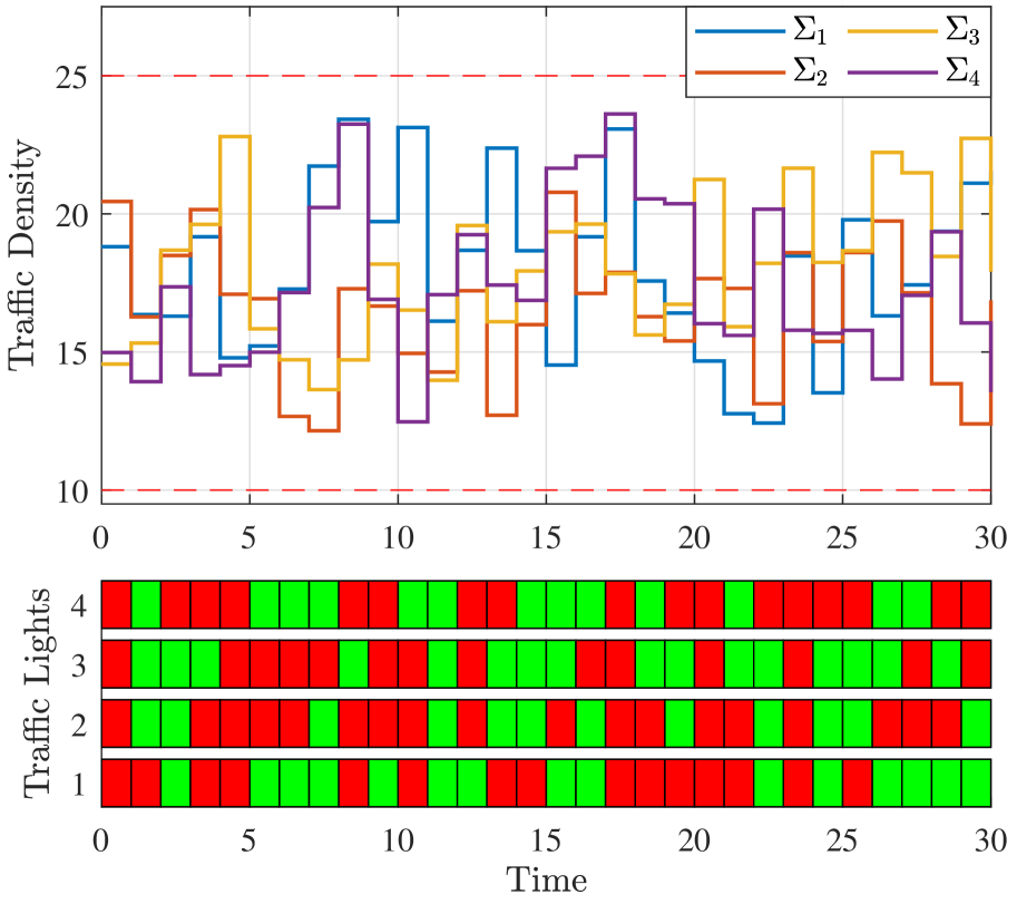
(d) Trajectories in subnetwork $\bar{G}_{4}$

Figure 2. Simulation results: Trajectories of traffic density (upper subplots) and traffic lights (lower subplots) in sample cells from different subnetworks. The traffic density in each cell (subsystem $\Sigma_{i}$) is required to remain in desired safe region $S_{i}$ (indicated by the red dashed lines). The sets $S_{i}$ are given by $S_{i}=[5,15]$ in subnetworks $\bar{G}_{1}$ and $\bar{G}_{2}$, $S_{i}=[10,25]$ in subnetworks $\bar{G}_{3}$ and $\bar{G}_{4}$.

5.3. Compositional safety controller synthesis

Now we synthesize a safety controller for the infinite network via the constructed symbolic model such that the density of traffic in each cell is maintained in a desired safe region. Specifically, we aim at finding a control policy such that in subnetworks $\bar{G}_{k}$, $k\in\{1,2\}$, each subsystem $\Sigma_{i}$ satisfies safety specification $S_{i}=[5,15]$ (vehicles per cell), and in subnetworks $\bar{G}_{k}$, $k\in\{3,4\}$, each subsystem $\Sigma_{i}$ satisfies safety specification $S_{i}=[10,25]$ (vehicles per cell). Note that for the overall network, the overall safety specification $S=\prod_{i\in\mathbb{N}}S_{i}$ is globally decomposable. By Proposition 18, one can design local safety controllers for the subsystems separately with respect to local safety specifications, with the guarantee that the composed controller works as the overall safety controller for the overall infinite network. For each subsystem $\Sigma_{i}$, the idea is to design a local safety controller for its symbolic model $\hat{\Sigma}_{i}$, and then refine the controller back to the original subsystem by choosing $u_{i}=\hat{u}_{i}$. The control strategies are correct-by-construction, in the sense that the safety specification is guaranteed to be satisfied from any initial condition in the safe region.

Here, we employ the software tool SCOTS [28] to compositionally construct symbolic models and compute local safety controllers for subsystems $\Sigma_{i}$ with quantization parameters $\eta^{x}_{i}=0.1$ and $\eta^{u}_{i}=0$, for each $i\in\mathbb{N}$. Computing symbolic models and synthesizing controllers for each subsystem took on average $0.006$s and $0.0004$s, respectively, on a PC with Intel Core i7 3.4 GHz CPU. For each subnetwork, we show in Figure 2 four sample state trajectories (upper plots of the sub-figures) and the corresponding input trajectories (lower plots of the sub-figures) of sample subsystems starting from random initial conditions. As can be seen in the figures, at each time step, the synthesized controllers react to the change in the density of the traffic in the corresponding cells by turning the traffic lights green/red. It can be observed that the density of the traffic using the synthesized controllers always remain in the desired safe regions.

6. Conclusion

In this paper, we proposed a methodology to compositionally construct symbolic models for infinite networks. To do this, we first introduced a notion of so-called alternating simulation functions that can be used to relate infinite networks. A compositional approach was then proposed to construct symbolic models locally for concrete subsystems under incremental input-to-state stability property. By leveraging max-type small-gain type conditions, we provided an algorithm as a guideline for the design of local quantization parameters, such that the symbolic model of the infinite network can satisfy any given desired approximation accuracy. A decentralized controller synthesis approach was presented to enforce safety properties on the overall infinite network. Finally, we applied our results on a road traffic network to verify the effectiveness of our compositionality results.

References

• [1] M. R. Jovanovic and B. Bamieh, “On the ill-posedness of certain vehicular platoon control problems,” IEEE Transactions on Automatic Control, vol. 50, no. 9, pp. 1307–1321, 2005.
• [2] B. Bamieh, F. Paganini, and M. A. Dahleh, “Distributed control of spatially invariant systems,” IEEE Transactions on Automatic Control, vol. 47, no. 7, pp. 1091–1107, 2002.
• [3] C. Kawan, A. Mironchenko, A. Swikir, N. Noroozi, and M. Zamani, “A Lyapunov-based small-gain theorem for infinite networks,” IEEE Transactions on Automatic Control, in press, 2021.
• [4] A. Mironchenko, C. Kawan, and J. Glück, “Nonlinear small-gain theorems for input-to-state stability of infinite interconnections,” arXiv preprint arXiv:2007.05705, 2020.
• [5] S. Dashkovskiy, A. Mironchenko, J. Schmid, and F. Wirth, “Stability of infinitely many interconnected systems,” in Proceedings of 11th IFAC Symposium on Nonlinear Control Systems.   Elsevier, 2019, pp. 937–942.
• [6] N. Noroozi, A. Mironchenko, and F. R. Wirth, “A relaxed small-gain theorem for discrete-time infinite networks,” in 59th IEEE Conference on Decision and Control, 2020, pp. 3102–3107.
• [7] A. Mironchenko and C. Prieur, “Input-to-state stability of infinite-dimensional systems: Recent results and open questions,” SIAM Review, vol. 62, no. 3, pp. 529–614, 2020.
• [8] S. Dashkovskiy and S. Pavlichkov, “Stability conditions for infinite networks of nonlinear systems and their application for stabilization,” Automatica, vol. 112, p. 108643, 2020.
• [9] A. Swikir, N. Noroozi, and M. Zamani, “Compositional synthesis of symbolic models for infinite networks,” in 21st IFAC World Congress, July 2020.
• [10] P. Tabuada, Verification and control of hybrid systems: a symbolic approach.   Boston, MA: Springer, 2009.
• [11] G. Pola and P. Tabuada, “Symbolic models for nonlinear control systems: Alternating approximate bisimulations,” SIAM Journal on Control and Optimization, vol. 48, no. 2, pp. 719–733, 2009.
• [12] G. Pola, A. Girard, and P. Tabuada, “Approximately bisimilar symbolic models for nonlinear control systems,” Automatica, vol. 44, no. 10, pp. 2508–2516, 2008.
• [13] C. Baier and J.-P. Katoen, Principles of model checking.   MIT press, 2008.
• [14] Y. Tazaki and J.-i. Imura, “Bisimilar finite abstractions of interconnected systems,” in International Workshop on Hybrid Systems: Computation and Control.   Springer, 2008, pp. 514–527.
• [15] G. Pola, P. Pepe, and M. D. D. Benedetto, “Symbolic models for networks of control systems,” IEEE Transactions on Automatic Control, vol. 61, no. 11, pp. 3663–3668, Nov. 2016.
• [16] M. Zamani and M. Arcak, “Compositional abstraction for networks of control systems: A dissipativity approach,” IEEE Transactions on Control of Network Systems, vol. 5, no. 3, pp. 1003–1015, 2018.
• [17] A. Swikir and M. Zamani, “Compositional synthesis of finite abstractions for networks of systems: A small-gain approach,” Automatica, vol. 107, no. 11, pp. 551 – 561, 2019.
• [18] K. Mallik, A.-K. Schmuck, S. Soudjani, and R. Majumdar, “Compositional synthesis of finite-state abstractions,” IEEE Transactions on Automatic Control, vol. 64, no. 6, pp. 2629–2636, 2018.
• [19] P. J. Meyer, A. Girard, and E. Witrant, “Compositional abstraction and safety synthesis using overlapping symbolic models,” IEEE Transactions on Automatic Control, vol. 63, no. 6, pp. 1835–1841, 2017.
• [20] E. S. Kim, M. Arcak, and M. Zamani, “Constructing control system abstractions from modular components,” in Proceedings of the 21st International Conference on Hybrid Systems: Computation and Control, 2018, pp. 137–146.
• [21] G. Pola, P. Pepe, M. D. Di Benedetto, and P. Tabuada, “Symbolic models for nonlinear time-delay systems using approximate bisimulations,” Systems & Control Letters, vol. 59, no. 6, pp. 365–373, 2010.
• [22] A. Girard, “Approximately bisimilar abstractions of incrementally stable finite or infinite dimensional systems,” in 53rd IEEE Conference on Decision and Control, 2014, pp. 824–829.
• [23] D. Angeli, “A Lyapunov approach to incremental stability properties,” IEEE Transactions on Automatic Control, vol. 47, no. 3, pp. 410–421, 2002.
• [24] M. Zamani, P. Mohajerin Esfahani, R. Majumdar, A. Abate, and J. Lygeros, “Symbolic control of stochastic systems via approximately bisimilar finite abstractions,” IEEE Transactions on Automatic Control, vol. 59, no. 12, pp. 3135–3150, 2014.
• [25] T. A. Henzinger, S. Qadeer, and S. K. Rajamani, “You assume, we guarantee: Methodology and case studies,” in Computer Aided Verification, 1998, pp. 440–451.
• [26] S. Liu and M. Zamani, “Compositional synthesis of almost maximally permissible safety controllers,” in American Control Conference, 2019, pp. 1678–1683.
• [27] C. Canudas-de Wit, L. L. Ojeda, and A. Y. Kibangou, “Graph constrained-ctm observer design for the grenoble south ring,” IFAC Proceedings Volumes, vol. 45, no. 24, pp. 197–202, 2012.
• [28] M. Rungger and M. Zamani, “SCOTS: A tool for the synthesis of symbolic controllers,” in Proceedings of the 19th International Conference on Hybrid Systems: Computation and Control.   ACM, Apr. 2016.