Abstract

Given the increasing promise of graph neural networks (GNNs) in real-world applications, several methods have been developed for explaining their predictions. Existing methods for interpreting predictions from GNNs have primarily focused on generating subgraphs that are especially relevant for a particular prediction. However, such methods are not counterfactual (CF) in nature: given a prediction, we want to understand how the prediction can be changed in order to achieve an alternative outcome. In this work, we propose a method for generating CF explanations for GNNs: the minimal perturbation to the input (graph) data such that the prediction changes. Using only edge deletions, we find that our method, CF-GNNExplainer, can generate CF explanations for the majority of instances across three widely used datasets for GNN explanations, while removing less than 3 edges on average, with at least 94% accuracy. This indicates that CF-GNNExplainer primarily removes edges that are crucial for the original predictions, resulting in minimal CF explanations.

1 INTRODUCTION

Advances in machine learning (ML) have led to breakthroughs in several areas of science and engineering, ranging from computer vision, to natural language processing, to conversational assistants. Parallel to the increased performance of ML systems, there is an increasing call for the “understandability” of ML models  (Goebel et al., 2018). Understanding why an ML model returns a certain output in response to a given input is important for a variety of reasons such as model debugging, aiding decison-making, or fulfilling legal requirements (EU, 2016). Having certified methods for interpreting ML predictions will help enable their use across a variety of applications (Miller, 2019).

Explainable AI (XAI) refers to the set of techniques “focused on exposing complex AI models to humans in a systematic and interpretable manner” (Samek et al., 2019). A large body of work on XAI has emerged in recent years (Guidotti et al., 2018b; Bodria et al., 2021). Counterfactual (CF) explanations are used to explain predictions of individual instances in the form: “If X had been different, Y would not have occurred” (Stepin et al., 2021; Karimi et al., 2020a; Schut et al., 2021). CF explanations are based on CF examples: modified versions of the input sample that result in an alternative output (i.e., prediction). If the proposed modifications are also actionable, this is referred to as achieving recourse (Ustun et al., 2019; Karimi et al., 2020b).

To motivate our problem, consider an ML application for computational biology: drug discovery is a task that involves generating new molecules that can be used for medicinal purposes (Stokes et al., 2020; Xie et al., 2021). Given a candidate molecule, a GNN can predict if this molecule has a certain property that would make it effective in treating a particular disease (Wieder et al., 2020; Guo et al., 2021; Nguyen et al., 2020). If the GNN predicts it does not have this desirable property, CF explanations can help identify the minimal change required such that the molecule is predicted to have this property. This could help not only inform the design of a new molecule that has this property, but also understand the molecular structures that contribute to this property.

Although GNNs have shown state-of-the-art results on tasks involving graph data (Zitnik et al., 2018; Deac et al., 2019), existing methods for explaining the predictions of GNNs have primarily focused on generating subgraphs that are relevant for a particular prediction (Yuan et al., 2020b; Baldassarre and Azizpour, 2019; Duval and Malliaros, 2021; Lin et al., 2021; Luo et al., 2020; Pope et al., 2019; Schlichtkrull et al., 2021; Vu and Thai, 2020; Ying et al., 2019; Yuan et al., 2021). However, none of these methods are able to identify the minimal subgraph automatically – they all require the user to specify the size of the subgraph, $S$, in advance. We show that even if we adapt existing methods to the CF explanation problem, and try varying values for $S$, such methods are not able to produce valid, accurate CF explanations, and are therefore not well-suited to solve the CF explanation problem. To address this gap, we propose CF-GNNExplainer, a method for generating CF explanations for GNNs.

Similar to other CF methods for tabular or image data proposed in the literature (Verma et al., 2020; Karimi et al., 2020b), CF-GNNExplainer works by perturbing input data at the instance-level. Unlike previous methods, CF-GNNExplainer can generate CF explanations for graph data. In particular, our method iteratively removes edges from the original adjacency matrix based on matrix sparsification techniques, keeping track of the perturbation that leads to a change in prediction, and returning the perturbation with the smallest change w.r.t. the number of edges.

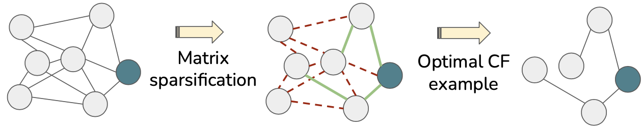
Figure 1: Intuition of counterfactual example generation by CF-GNNExplainer.

We evaluate CF-GNNExplainer on three public datasets for GNN explanations and measure its effectiveness using four metrics: fidelity, explanation size, sparsity, and accuracy. We find that CF-GNNExplainer is able to generate CF examples with at least 94% accuracy, while removing fewer than 3 edges on average. We make the following contributions:

• We formalize the problem of generating CF explanations for GNNs (Section 4).

• We propose CF-GNNExplainer, a novel method for explaining predictions from GNNs (Section 5).

• We propose an experimental setup for holistically evaluating CF explanations for GNNs (Section 6).

The implementation of CF-GNNExplainer is available at https://github.com/cf-gnnexplainer.

2 RELATED WORK

Since our work is a counterfactual XAI approach for GNNs, it is related to GNN explainability (Section 2.1) as well as counterfactual explanations (Section 2.2). It is also related to adversarial attack methods (Section 2.3).

2.1 GNN Explainability

Several GNN XAI approaches have been proposed – a recent survey of the most relevant work is presented by Yuan et al. (2020b). However, unlike our work, none of the methods in this survey generate CF explanations.

The majority of existing GNN XAI methods provide an explanation in the form of a subgraph of the original graph that is deemed to be important for the prediction (Yuan et al., 2020b; Baldassarre and Azizpour, 2019; Duval and Malliaros, 2021; Lin et al., 2021; Luo et al., 2020; Pope et al., 2019; Schlichtkrull et al., 2021; Vu and Thai, 2020; Ying et al., 2019; Yuan et al., 2021). We refer to these as subgraph-generating methods. Such methods are analogous to popular XAI methods such as LIME (Ribeiro et al., 2016) or SHAP (Lundberg and Lee, 2017), which identify relevant features for a particular prediction for tabular, image, or text data. All of these methods require the user to specify the size of the explanation, $S$, in advance: the number of features (or edges) to keep. In contrast, CF-GNNExplainer generates CF explanations, which can find the size of the explanation without requiring input from the user. Although both types of techniques are meant for explaining GNN predictions, they are solving fundamentally different problems: CF explanations generate the minimal perturbation such that the prediction changes, while subgraph-retrieving methods identify a relevant (and not necessarily minimal) subgraph that matches the original prediction.

Kang et al. (2019) also generate CF examples for GNNs, but their work focuses on a different task: link prediction. Other GNN XAI methods identify important node features (Huang et al., 2020) or similar examples (Faber et al., 2020). Yuan et al. (2020a) and Schnake et al. (2020) generate model-level (i.e., global) explanations for GNNs, which differs from our work since we produce instance-level (i.e., local) explanations.

2.2 Counterfactual Explanations

There exists a substantial body of work on CF explanations for tabular, image, and text data (Verma et al., 2020; Karimi et al., 2020b; Stepin et al., 2021). Some methods treat the underlying classification model as a black-box (Laugel et al., 2018; Guidotti et al., 2018a; Lucic et al., 2020), whereas others make use of the model’s inner workings (Tolomei et al., 2017; Wachter et al., 2018; Ustun et al., 2019; Kanamori et al., 2020; Lucic et al., 2022). All of these methods are based on perturbing feature values to generate CF examples – they are not equipped to handle graph data with relationships (i.e., edges) between instances (i.e., nodes). In contrast, CF-GNNExplainer provides CF examples specifically for graph data.

2.3 Adversarial Attacks

CF examples are also related to adversarial attacks (Sun et al., 2018): they both represent instances obtained from minimal perturbations to the input, which induce changes in the prediction made by the learned model. One difference between the two is in the intent: adversarial examples are meant to fool the model, while CF examples are meant to explain the prediction (Freiesleben, 2021; Lucic et al., 2022). In the context of graph data, adversarial attack methods typically make minimal perturbations to the overall graph with the intention of degrading overall model performance, as opposed to attacking individual nodes. In contrast, we are interested in generating CF examples for individual nodes, as opposed to identifying perturbations to the overall graph. We confirm that the CF examples produced by CF-GNNExplainer are informative and not adversarial by measuring the accuracy of our method (see Section 6.3).

3 BACKGROUND

In this section, we provide background information on GNNs (Section 3.1) and matrix sparsification (Section 3.2), both of which are necessary for understanding CF-GNNExplainer.

3.1 Graph Neural Networks

Graphs are structures that represent a set of entities (nodes) and their relations (edges). GNNs operate on graphs to produce representations that can be used in downstream tasks such as graph or node classification. The latter is the focus of this work. We refer to the survey papers by Battaglia et al. (2018) and Chami et al. (2021) for an overview of existing GNN methods.

Let $f(A,X;W)\rightarrow y$ be any GNN, where $y$ is the set of possible predicted classes, $A$ is an $n\times n$ adjacency matrix, $X$ is an $n\times p$ feature matrix, and $W$ is the learned weight matrix of $f$. In other words, $A$ and $X$ are the inputs of $f$, and $f$ is parameterized by $W$.

A node’s representation is learned by iteratively updating the node’s features based on its neighbors’ features. The number of layers in $f$ determines which neighbors are included: if there are $\ell$ layers, then the node’s final representation only includes neighbors that are at most $\ell$ hops away from that node in the graph $\mathcal{G}$. The rest of the nodes in $\mathcal{G}$ are not relevant for the computation of the node’s final representation. We define the subgraph neighborhood of a node $v$ as the set of the nodes and edges relevant for the computation of $f(v)$ (i.e., those in the $\ell$-hop neighborhood of $f$), represented as a tuple: $\mathcal{G}_{v}=(A_{v},X_{v})$, where $A_{v}$ is the subgraph adjacency matrix and $X_{v}$ is the node feature matrix for nodes that are at most $\ell$ hops away from $v$. We then define a node $v$ as a tuple of the form $v=(A_{v},x)$, where $x$ is the feature vector for $v$.

3.2 Matrix Sparsification

CF-GNNExplainer uses matrix sparsification to generate CF examples, inspired by Srinivas et al. (2017), who propose a method for training sparse neural networks. Given a weight matrix $W$, a binary sparsification matrix is learned which is multiplied element-wise with $W$ such that some of the entries in $W$ are zeroed out. In the work by Srinivas et al. (2017), the objective is to remove entries in the weight matrix in order to reduce the number of parameters in the model. In our case, we want to zero out entries in the adjacency matrix (i.e., remove edges) in order to generate CF explanations for GNNs. That is, we want to remove the important edges – those that are crucial for the prediction.

4 PROBLEM FORMULATION

In general, a CF example $\bar{x}$ for an instance $x$ according to a trained classifier $f$ is found by perturbing the features of $x$ such that $f(x)\neq f(\bar{x})$ (Wachter et al., 2018). An optimal CF example $\bar{x}^{*}$ is one that minimizes the distance between the original instance and the CF example, according to some distance function $d$, and the resulting optimal CF explanation is $\Delta^{*}_{x}=\bar{x}^{*}-x$ (Lucic et al., 2022).

For graph data, it may not be enough to simply perturb node features, especially since they are not always available. This is why we are interested in generating CF examples by perturbing the graph structure instead. In other words, we want to change the relationships between instances (i..e, nodes), rather than change the instances themselves. Therefore, a CF example for graph data has the form $\bar{v}=(\bar{A_{v}},x)$, where $x$ is the feature vector and $\bar{A_{v}}$ is a perturbed version of $A_{v}$, the adjacency matrix of the subgraph neighborhood of a node $v$. $\bar{A_{v}}$ is obtained by removing some edges from $A_{v}$, such that $f(v)\neq f(\bar{v})$. Following Wachter et al. (2018) and Lucic et al. (2022), we generate CF examples by minimizing a loss function of the form:

$$\mathcal{L}=\mathcal{L}_{pred}(v,\bar{v}\mid f,g)+\beta\mathcal{L}_{dist}(v,\bar{v}\mid d),$$ (1)

where $v$ is the original node, $f$ is the original model, $g$ is the CF model that generates $\bar{v}$, and $\mathcal{L}_{pred}$ is a prediction loss that encourages $f(v)\neq f(\bar{v})$. $\mathcal{L}_{dist}$ is a distance loss that encourages $\bar{v}$ to be close to $v$, and $\beta$ controls how important $\mathcal{L}_{dist}$ is compared to $\mathcal{L}_{pred}$. We want to find $\bar{v}^{*}$ that minimizes Eq. 1: this is the optimal CF example for $v$.

5 METHOD: CF-GNNExplainer

To solve the problem defined in Section 4, we propose CF-GNNExplainer, which generates $\bar{v}=(\bar{A_{v}},x)$ given a node $v=(A_{v},x)$. Our method can operate on any GNN model $f$. To illustrate our method and avoid cluttered notation, let $f$ be a standard, one-layer Graph Convolutional Network (Kipf and Welling, 2017) for node classification:

$$f(A,X;W)=\operatorname{softmax}\left[\tilde{D}^{-1/2}\tilde{A}\tilde{D}^{-1/2}XW\right],$$ (2)

where $\tilde{A}=A+I$, $I$ is the identity matrix, $\tilde{D}_{ii}=\sum_{j}\tilde{A}_{ij}$ are entries in the degree matrix $\tilde{D}$, $X$ is the node feature matrix, and $W$ is the weight matrix (Kipf and Welling, 2017).

5.1 Adjacency Matrix Perturbation

First, we define $\bar{A_{v}}=P\odot A_{v}$, where $P$ is a binary perturbation matrix that sparsifies $A_{v}$. Our aim is to find $P$ for a given node $v$ such that $f(A_{v},x)\neq f(P\odot A_{v},x$). To find $P$, we build upon the method by Srinivas et al. (2017) for training sparse neural networks (see Section 3), where our objective is to zero out entries in the adjacency matrix (i.e., remove edges). That is, we want to find $P$ that minimally perturbs $A_{v}$, and use it to compute $\bar{A_{v}}=P\odot A_{v}$. If an element $P_{{i,j}}=0$, this results in the deletion of the edge between node $i$ and node $j$. When $P$ is a matrix of ones, this indicates that all edges in $A_{v}$ are used in the forward pass.

Similar to the work by Srinivas et al. (2017), we first generate an intermediate, real-valued matrix $\hat{P}$ with entries in $\left[0,1\right]$, apply a sigmoid transformation, then threshold the entries to arrive at a binary $P$: entries greater than or equal to 0.5 become 1, while those below 0.5 become 0. In the case of undirected graphs (i.e., those with symmetric adjacency matrices), we first generate a perturbation vector which we then use to populate $\hat{P}$ in a symmetric manner, instead of generating $\hat{P}$ directly.

5.2 Counterfactual Generating Model

We want our perturbation matrix $P$ to only act on $A_{v}$, not $\tilde{A_{v}}$, in order to preserve self-loops in the message passing of $f$. This is because we always want a node representation update to include its own representation from the previous layer. Therefore we first rewrite Eq. 2 for our illustrative one-layer case to isolate $A_{v}$:

$$\begin{split}&\mbox{}f(A_{v},X_{v};W)=\\ &\mbox{}\operatorname{softmax}\left[(D_{v}+I)^{-1/2}(A_{v}+I)(D_{v}+I)^{-1/2}X_{v}W\right]\mbox{}\end{split}$$ (3)

To generate CFs, we propose a new function $g$, which is based on $f$, but it is parameterized by $P$ instead of $W$. We update the degree matrix $D_{v}$ based on $P\odot A_{v}$, add the identity matrix to account for self-loops (as in $\tilde{D_{v}}$ in Eq. 2), and call this $\bar{D_{v}}$:

$$\begin{split}&g(A_{v},X_{v},W;P)=\\ &\operatorname{softmax}\left[\bar{D_{v}}^{-1/2}(P\odot A_{v}+I)\bar{D_{v}}^{-1/2}X_{v}W\right]\end{split}$$ (4)

In other words, $f$ learns the weight matrix while holding the data constant, while $g$ generates new data points (i.e., CF examples) while holding the weight matrix (i.e., model) constant. Another distinction between $f$ and $g$ is that the aim of $f$ is to find the optimal set of weights that generalizes well on an unseen test set, while the objective of $g$ is to generate an optimal CF example, given a particular node (i.e., $\bar{v}$ is the output of $g$).

5.3 Loss Function Optimization

We generate $P$ by minimizing Eq. 1, adopting the negative log-likelihood (NLL) loss for $\mathcal{L}_{pred}$:

$$\begin{split}&\mathcal{L}_{pred}(v,\bar{v}|f,g)={}\\ &-\mathds{1}\left[f(v)=f(\bar{v})\right]\cdot\mathcal{L}_{NLL}(f(v),g(\bar{v})).\end{split}$$ (5)

Since we do not want $f(\bar{v})$ to match $f(v)$, we put a negative sign in front of $\mathcal{L}_{pred}$ and include an indicator function to ensure the loss is active as long as $f(\bar{v})=f(v)$. Note that $f$ and $g$ have the same weight matrix $W$ – the main difference is that $g$ also includes the perturbation matrix $P$.

$\mathcal{L}_{dist}$ can be based on any differentiable distance function. In our case, we take $d$ to be the element-wise difference between $v$ and $\bar{v}$, corresponding to the difference between $A_{v}$ and $\bar{A_{v}}$: the number of edges removed. For undirected graphs, we divide this value by 2 to account for the symmetry in the adjacency matrices. When updating $P$, we take the gradient of Eq. 1 with respect to the intermediate $\hat{P}$, not the binary $P$.

Algorithm 1 CF-GNNExplainer: given a node $v=(A_{v},x)$ where $f(v)=y$, generate the minimal perturbation, $\bar{v}=(\bar{A_{v}},x)$, such that $f(\bar{v})\neq y$.

  Input: node $v=(A_{v},x)$, trained GNN model $f$, CF model $g$, loss function $\mathcal{L}$, learning rate $\alpha$, number of iterations $K$, distance function $d$.

  

  $f(v)=y$ # Get GNN prediction

  $\hat{P}\leftarrow J_{n}$ # Initialization

  $\bar{v}^{*}=\left[\>\right]$

  

  for $K$ iterations do

     $\bar{v}$ = get_cf_example()

     $\mathcal{L}\leftarrow\mathcal{L}(v,\bar{v},f,g)$ # Eq 1 & Eq 5

     $\hat{P}\leftarrow\hat{P}+\alpha\nabla_{\hat{P}}\mathcal{L}$ # Update $\hat{P}$

  end for

  

  Function get_cf_example()

  $P\leftarrow\text{threshold}(\sigma(\hat{P}))$

  $\bar{A_{v}}\leftarrow P\odot A_{v}$

  $\bar{v}_{cand}\leftarrow(\bar{A_{v}},x)$

  if $f(v)\neq f(\bar{v}_{cand})$ then

        $\bar{v}\leftarrow\bar{v}_{cand}$

        if not $\bar{v}^{*}$ then

              $\bar{v}^{*}\leftarrow\bar{v}$ # First CF

        else if $d(v,\bar{v})\leq d(v,\bar{v}^{*})$ then

              $\bar{v}^{*}\leftarrow\bar{v}$ # Keep track of best CF

        end if

  end if

  return  $\bar{v}^{*}$

5.4 CF-GNNExplainer

We call our method CF-GNNExplainer and summarize its details in Algorithm 1. Given an node in the test set $v$, we first obtain its original prediction from $f$ and initialize ${\hat{P}}$ as a matrix of ones, $J_{n}$, to initially retain all edges. Next, we run CF-GNNExplainer for $K$ iterations. To find a CF example, we use Eq. LABEL:eq:cf.

First, we compute $P$ by thresholding $\hat{P}$ (see Section 5.1). Then we use $P$ to obtain the sparsified adjacency matrix that gives us a candidate CF example, $\bar{v}_{cand}$. This example is then fed to the original GNN, $f$, and if $f$ predicts a different output than for the original node, we have found a valid CF example, $\bar{v}$. We keep track of the “best” CF example (i.e., the most minimal according to $d$), and return this as the optimal CF example $\bar{v}^{*}$ after $K$ iterations. Between iterations, we compute the loss following Eqn 1 and 5, and update $\hat{P}$ based on the gradient of the loss. In the end, we retrieve the optimal CF explanation $\Delta_{v}^{*}=v-\bar{v}^{*}$.

5.5 Complexity

CF-GNNExplainer has time complexity $O(KN^{2})$, where $N$ is the number of nodes in the subgraph neighbourhood and $K$ is the number of iterations. We note that high complexity is common for local XAI methods (i.e., SHAP, GNNExplainer, etc), but in practice, one typically only generates explanations for a subset of the dataset.

6 EXPERIMENTAL SETUP

In this section, we outline our experimental setup for evaluating CF-GNNExplainer, including the datasets and models used (Section 6.1), the baselines we compare against (Section 6.2), the evaluation metrics (Section 6.3), and the hyperparameter search method (Section 6.4). In total, we run approximately 375 hours of experiments on one Nvidia TitanX Pascal GPU with access to 12GB RAM.

6.1 Datasets and Models

Given the challenges associated with defining and evaluating the accuracy of XAI methods (Doshi-Velez and Kim, 2018), we first focus on synthetic tasks where we know the ground-truth explanations. Although there exist real graph classification datasets with ground-truth explanations (Debnath et al., 1991), there do not exist any real node classification datasets with ground-truth explanations, which is the task we focus on in this paper. Building such a dataset would be an excellent contribution, but is outside the scope of this paper.

In our experiments, we use the tree-cycles, tree-grids, ba-shapes datasets from Ying et al. (2019). These datasets were created specifically for the task of explaining node classification predictions from GNNs. Each dataset consists of (i) a base graph, (ii) motifs that are attached to random nodes of the base graph, and (iii) additional edges that are randomly added to the overall graph. They are all undirected graphs. The classification task is to determine whether or not the nodes are part of the motif. The purpose of these datasets is to have a ground-truth for the “correctness” of an explanation: for nodes in the motifs, the explanation is the motif itself (Luo et al., 2020). The dataset statistics are available in Table 1.

tree-cycles consists of a binary tree base graph with 6-cycle motifs, tree-grids also has a binary tree as its base graph, but with 3$\times$3 grids as the motifs. For ba-shapes, the base graph is a Barabasi-Albert (BA) graph with house-shaped motifs, where each motif consists of 5 nodes (one for the top of the house, two in the middle, and two on the bottom). Here, there are four possible classes (not in motif, in motif: top, middle, bottom). We note that compared to the other two datasets, the ba-shapes dataset is much more densely connected – the node degree is more than twice as high as that of the tree-cycles or tree-grid datasets, and the average number of nodes and edges in each node’s computation graph is order(s) of magnitude larger. We use the same experimental setup (i.e., dataset splits, model architecture) as Ying et al. (2019) to train a 3-layer GCN (hidden size = 20) for each task. Our GCNs have at least 87% accuracy on the test set.

Table 1: Dataset statistics. The # edges in the motif indicates the size of the ground truth (GT) explanation.

	Tree	Tree	BA
	Cycles	Grid	Shapes
# classes	2	2	4
# nodes in motif	6	9	5
# edges in motif (GT)	6	12	6
# nodes in total	871	1231	700
# edges in total	1950	3410	4100
Avg node degree	2.27	2.77	5.87
Avg # nodes in $A_{v}$	19.12	30.69	304.40
Avg # edges in $A_{v}$	18.99	33.94	1106.24

6.2 Baselines

Since existing GNN XAI methods give explanations in the form of relevant subgraphs as opposed to CF examples, it is not straightforward to identify baselines for our experiments that ensure a fair comparison between methods. To evaluate CF-GNNExplainer, we compare against 4 baselines: random, 1hop, rm-1hop, and GNNExplainer. The random perturbation is meant as a sanity check. We randomly initialize the entries of $\hat{P}\in\left[-1,1\right]$ and apply the same sigmoid transformation and thresholding as described in Section 5.1. We repeat this $K$ times and keep track of the most minimal perturbation resulting in a CF example. Next, we compare against baselines that are based on the ego graph of $v$ (i.e., its 1-hop neighbourhood): 1hop keeps all edges in the ego graph of $v$, while rm-1hop removes all edges in the ego graph of $v$.

Our fourth baseline is based on GNNExplainer by Ying et al. (2019), which identifies the $S$ most relevant edges for the prediction (i.e., the most relevant subgraph of size $S$). To generate CF explanations, we remove the subgraph generated by GNNExplainer. We include this method in our experiments in order to have a baseline based on a prominent GNN XAI method, but we note that subgraph-retrieving methods like GNNExplainer are not meant for generating CF explanations. Unlike our method, GNNExplainer cannot automatically find a minimal subgraph and therefore requires the user to determine the number of edges to keep in advance (i.e., the value of $S$). As a result, we cannot evaluate how minimal its CF explanations are, but we can compare it against our method in terms of (i) its ability to generate valid CF examples, and (ii) how accurate those CF examples are. We report results on GNNExplainer for $S\in\{1,2,3,4,5,$ GT$\}$, where GT is the size of the ground truth explanation (i.e., the number of edges in the motif, see Table 1).

6.3 Metrics

We generate a CF example for each node in the graph separately and evaluate in terms of four metrics.

Fidelity: is defined as the proportion of nodes where the original predictions match the prediction for the explanations (Molnar, 2019; Ribeiro et al., 2016). Since we generate CF examples, we do not want the original prediction to match the prediction for the explanation, so we want a low value for fidelity.

Explanation Size: is the number of removed edges. It corresponds to the $\mathcal{L}_{dist}$ term in Equation 1: the difference between the original $A_{v}$ and the counterfactual $\bar{A_{v}}$. Since we want to have minimal explanations, we want a small value for this metric. Note that we cannot evaluate this metric for GNNExplainer.

Sparsity: measures the proportion of edges in $A_{v}$ that are removed (Yuan et al., 2020b). A value of 0 indicates all edges in $A_{v}$ were removed. Since we want minimal explanations, we want a value close to 1. Note that we cannot evaluate this metric for GNNExplainer.

Accuracy: is the mean proportion of explanations that are “correct”. Following Ying et al. (2019) and Luo et al. (2020), we only compute accuracy for nodes that are originally predicted as being part of the motifs, since accuracy can only be computed on instances for which we know the ground truth explanations. Given that we want minimal explanations, we consider an explanation to be correct if it exclusively involves edges that are inside the motifs (i.e., only removes edges that are within the motifs).

The exact calculations of all metrics can be found in the public code base at https://github.com/cf-gnnexplainer.

Table 2: Results comparing our method to random, 1hop, and rm-1hop. Below each metric, $\blacktriangledown$ indicates a low value is desirable, while $\blacktriangle$ indicates a high value is desirable.

	tree-cycles				tree-grid				ba-shapes
	Fid.	Size	Spars.	Acc.	Fid.	Size	Spars.	Acc.	Fid.	Size	Spars.	Acc.
Method	$\blacktriangledown$	$\blacktriangledown$	$\blacktriangle$	$\blacktriangle$	$\blacktriangledown$	$\blacktriangledown$	$\blacktriangle$	$\blacktriangle$	$\blacktriangledown$	$\blacktriangledown$	$\blacktriangle$	$\blacktriangle$
random	0.00	4.70	0.79	0.63	0.00	9.06	0.75	0.77	0.00	503.31	0.58	0.17
1hop	0.32	15.64	0.13	0.45	0.32	29.30	0.09	0.72	0.60	504.18	0.05	0.18
rm-1hop	0.46	2.11	0.89	—	0.61	2.27	0.92	—	0.21	10.56	0.97	0.99
CF-GNNExplainer	0.21	2.09	0.90	0.94	0.07	1.47	0.94	0.96	0.39	2.39	0.99	0.96

6.4 Hyperparameter Search

We experiment with different optimizers and hyperparameter values for the number of iterations $K$, the trade-off parameter $\beta$, the learning rate $\alpha$, and the Nesterov momentum $m$ (when applicable). We choose the setting that produces the most CF examples. We test the number of iterations $K\in\{100,300,500\}$, the trade-off parameter $\beta\in\{0.1,0.5\}$, the learning rate $\alpha\in\{0.005,0.01,0.1,1\}$, and the Nesterov momentum $m\in\{0,0.5,0.7,0.9\}$. We test Adam, SGD and AdaDelta as optimizers. We find that for all three datasets, the SGD optimizer gives the best results, with $k=500$, $\beta=0.5$, and $\alpha=0.1$. For the tree-cycles and tree-grid datasets, we set $m=0$, while for the ba-shapes dataset, we use $m=0.9$.

7 RESULTS

We evaluate CF-GNNExplainer in terms of the metrics outlined in Section 6.3. The results are shown in Table 2 and Table 3. In almost all settings, we find that CF-GNNExplainer outperforms the baselines in terms of explanation size, sparsity, and accuracy, which shows that CF-GNNExplainer satisfies our objective of finding accurate, minimal CF examples. In cases where the baselines outperform CF-GNNExplainer on a particular metric, they perform poorly on the rest of the metrics, or on other datasets.

7.1 Main Findings

Fidelity: CF-GNNExplainer outperforms 1hop across all three datasets, and outperforms rm-1hop for tree-cycles and tree-grid in terms of fidelity. We find that random has the lowest fidelity in all cases – it is able to find CF examples for every single node. In the following subsections, we will see that this corresponds to poor performance on the other metrics.

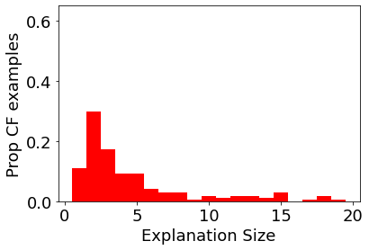
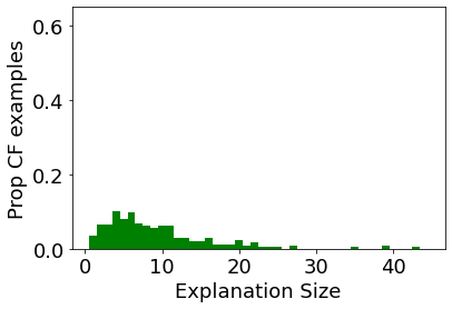
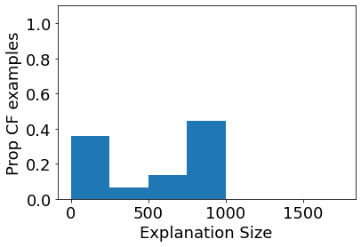
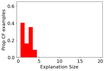
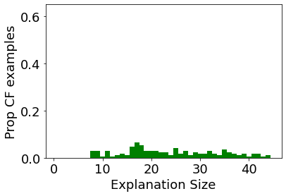
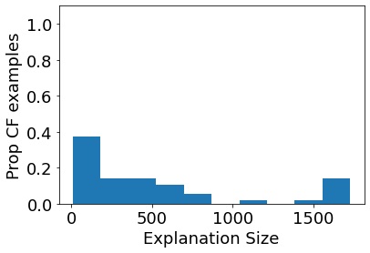
Figure 2: Histograms showing the proportion of CF examples that have a certain explanation size from random. Note the $x$-axis for ba-shapes goes up to 1500. Left: tree-cycles, Middle: tree-grid, Right: ba-shapes.

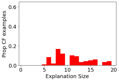
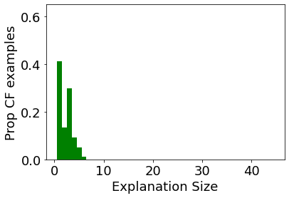
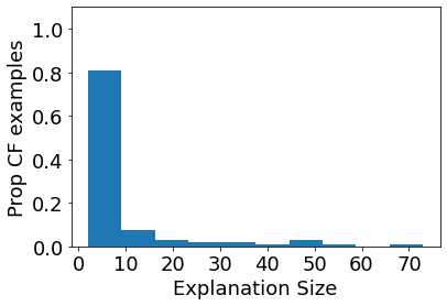
Figure 3: Histograms showing the proportion of CF examples that have a certain explanation size from 1hop. Note the $x$-axis for ba-shapes goes up to 1500. Left: tree-cycles, Middle: tree-grid, Right: ba-shapes.

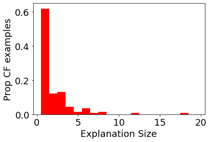
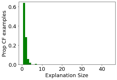
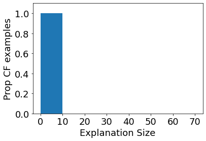
Figure 4: Histograms showing the proportion of CF examples that have a certain explanation size from rm-1hop. Note the $x$-axis for ba-shapes goes up to 70. Left: tree-cycles, Middle: tree-grid, Right: ba-shapes.

Figure 5: Histograms showing the proportion of CF examples that have a certain explanation size from CF-GNNExplainer. Note the $x$-axis for ba-shapes goes up to 70. Left: tree-cycles, Middle: tree-grid, Right: ba-shapes.

Explanation Size: Figures 5 to 5 show histograms of the explanation size for CF-GNNExplainer and the baselines.

We see that across all three datasets, CF-GNNExplainer has the smallest (i.e., most minimal) explanation sizes. This is especially true when comparing to random and 1hop for the ba-shapes dataset, where we had to use a different scale for the $x$-axis due to how different the explanation sizes were. We postulate that this difference could be because ba-shapes is a much more densely connected graph; it has fewer nodes but more edges compared to the other two datasets, and the average number of nodes and edges in the subgraph neighborhood is order(s) of magnitude larger (see Table 1). Therefore, when performing random perturbations, there is substantial opportunity to remove edges that do not necessarily need to be removed, leading to much larger explanation sizes. When there are many edges in the subgraph neighborhood, removing everything except the 1-hop neighbourhood, as is done in 1hop, also results in large explanation sizes. In contrast, the loss function used by CF-GNNExplainer ensures that only a few edges are removed, which is the desirable behavior since we want minimal explanations.

Sparsity: CF-GNNExplainer outperforms the random, rm-1hop, 1hop baselines for all three datasets in terms of sparsity. We note CF-GNNExplainer and rm-1hop perform much better on this metric in comparison to the other methods, which aligns with the results from explanation size.

Accuracy: We observe that CF-GNNExplainer has the highest accuracy for the tree-cycles and tree-grid datasets, whereas rm-1hop has the highest accuracy for ba-shapes. However, we are unable to calculate the accuracy of rm-1hop for the other two datasets since it is unable to generate any CF examples for motif nodes, contributing to the low sparsity on those datasets. We observe accuracy levels upwards of 94% for CF-GNNExplainer across all datasets, indicating that it is consistent in correctly removing edges that are crucial for the initial predictions in the vast majority of cases (see Table 2).

Table 3: Results comparing our method to GNNExplainer. GNNExplainer cannot find $S$ automatically, so we try varying values of $S$. GT indicates the size of the ground truth explanation for each dataset. CF-GNNExplainer finds $S$ automatically. Below each metric, $\blacktriangledown$ indicates a low value is desirable, while $\blacktriangle$ indicates a high value is desirable.

	tree-cycles				tree-grid				ba-shapes
	Fid.	Size	Spars.	Acc.	Fid.	Size	Spars.	Acc.	Fid.	Size	Spars.	Acc.
Method	$\blacktriangledown$	$\blacktriangledown$	$\blacktriangle$	$\blacktriangle$	$\blacktriangledown$	$\blacktriangledown$	$\blacktriangle$	$\blacktriangle$	$\blacktriangledown$	$\blacktriangledown$	$\blacktriangle$	$\blacktriangle$
GNNExp ($S=1$)	0.65	1.00	0.92	0.61	0.69	1.00	0.96	0.79	0.90	1.00	0.94	0.52
GNNExp ($S=2$)	0.59	2.00	0.85	0.54	0.51	2.00	0.92	0.78	0.85	2.00	0.91	0.40
GNNExp ($S=3$)	0.56	3.00	0.79	0.51	0.46	3.00	0.88	0.79	0.83	3.00	0.87	0.34
GNNExp ($S=4$)	0.58	4.00	0.72	0.48	0.42	4.00	0.84	0.79	0.83	4.00	0.83	0.31
GNNExp ($S=5$)	0.57	5.00	0.66	0.46	0.40	5.00	0.80	0.79	0.81	5.00	0.81	0.27
GNNExp ($S=$ GT)	0.55	6.00	0.57	0.46	0.35	11.83	0.53	0.74	0.82	6.00	0.79	0.24
CF-GNNExplainer	0.21	2.09	0.90	0.94	0.07	1.47	0.94	0.96	0.39	2.39	0.99	0.96

7.2 Comparison to GNNExplainer

Table 3 shows the results comparing our method to GNNExplainer. We find that our method outperforms GNNExplainer across all three datasets in terms of both fidelity and accuracy, for all tested values of $S$. However, this is not surprising since GNNExplainer is not meant for generating CF explanations, so we cannot expect it to perform well on a task it was not designed for. We cannot compare explanation size or sparsity fairly since GNNExplainer requires the user to input the value of $S$.

7.3 Summary of results

Evaluating on four distinct metrics for each dataset gives us a more holistic view of the results. We find that across all three datasets, CF-GNNExplainer can generate CF examples for the majority of nodes in the test set (i.e., low fidelity), while only removing a small number of edges (i.e., low explanation size, high sparsity). For nodes where we know the ground truth (i.e., those in the motifs) we achieve at least 94% accuracy.

Although random can generate CF examples for every node, they are not very minimal or accurate. The latter is also true for 1hop – in general, it has the worst scores for explanation size, sparsity and accuracy. GNNExplainer performs at a similar level as 1hop, indicating that although it is a prominent GNN XAI method, it is not well-suited for solving the CF explanation problem.

rm-1hop is competitive in terms of explanation size, but it performs poorly in terms of fidelity for the tree-cycles and tree-grid datasets, and its accuracy on these datasets is unknown since it is unable to generate any CF examples for nodes in the motifs. These results show that our method is simple and extremely effective in solving the CF explanation task, unlike the baselines we test.

8 SOCIETAL IMPACT

Researchers have raised concerns about the hidden assumptions behind the use of CF examples (Barocas et al., 2020), as well as potentials for misuse (Kasirzadeh and Smart, 2021). When explaining ML systems through CF examples, it is crucial to account for the context in which the system is deployed. CF explanations are not a guarantee to achieving recourse (Ustun et al., 2019) – changes suggested should be seen as candidate changes, not absolute solutions, since what is pragmatically actionable differs depending on the context.

We believe it is crucial for the ML community to invest in developing more rigorous evaluation protocols for XAI methods. We suggest that researchers in XAI collaborate with researchers in human-computer interaction to design human-centered user studies about evaluating the utility of XAI methods in practice. We are glad to see initiatives for such collaborations already taking place (Ehsan et al., 2021).

9 CONCLUSION

In this work, we propose CF-GNNExplainer, a method for generating CF explanations for any GNN. Our simple and effective method is able to generate CF explanations that are (i) minimal, both in terms of the absolute number of edges removed (explanation size), as well as the proportion of the subgraph neighborhood that is perturbed (sparsity), and (ii) accurate, in terms of removing edges that we know to be crucial for the initial predictions.

We evaluate our method on three commonly used datasets for GNN explanation tasks and find that these results hold across all three datasets. We find that existing GNN XAI methods are not well-suited to solving the CF explanation task, while CF-GNNExplainer is able to reliably produce minimal, accurate CF explanations.

In its current form, CF-GNNExplainer is limited to performing edge deletions in the context of node classification tasks. For future work, we plan to incorporate node feature perturbations in our framework and extend CF-GNNExplainer to accommodate graph classification tasks. We also plan to investigate adapting graph attack methods for generating CF explanations, as well as conduct a user study to determine if humans find CF-GNNExplainer useful in practice.

Acknowledgements

We want to thank Li Chen as well as the anonymous reviewers for the thoughtful feedback they provided on the paper. This research was supported by the Netherlands Organisation for Scientific Research (NWO) under project nr. 652.001.003, the Dutch National Police, the Italian Ministry of Education, University and Research (MIUR) under the grant “Dipartimenti di eccellenza 2018-2022” of the Department of Computer Science and the Department of Computer Engineering at Sapienza University of Rome. All content represents the opinion of the authors, which is not necessarily shared or endorsed by their respective employers and/or sponsors.

 

Supplementary Material:
CF-GNNExplainer: Counterfactual Explanations for Graph Neural Networks

 

Appendix A Results Table Including Standard Deviations

Here we show Table 2 from the manuscript including standard deviations. We report standard deviation for two metrics: Explanation Size and Sparsity, since both of these involve taking the mean over the entire dataset. Standard deviation does not apply to Fidelity or Accuracy because these metrics represent a proportion as opposed to a mean.

Table 2: Results comparing our method (denoted CF-GNN) to random, 1hop, and rm-1hop. Below each metric, $\blacktriangledown$ indicates a low value is desirable, while $\blacktriangle$ indicates a high value is desirable.

	tree-cycles				tree-grid				ba-shapes
	Fid.	Size	Spars.	Acc.	Fid.	Size	Spars.	Acc.	Fid.	Size	Spars.	Acc.
Method	$\blacktriangledown$	$\blacktriangledown$	$\blacktriangle$	$\blacktriangle$	$\blacktriangledown$	$\blacktriangledown$	$\blacktriangle$	$\blacktriangle$	$\blacktriangledown$	$\blacktriangledown$	$\blacktriangle$	$\blacktriangle$
random	0.00	4.70 $\pm$ 4.28	0.79 $\pm$ 0.07	0.63	0.00	9.06 $\pm$ 6.81	0.75 $\pm$ 0.07	0.77	0.00	503.31 $\pm$ 332.61	0.58 $\pm$ 0.10	0.17
1hop	0.32	15.64 $\pm$ 12.36	0.13 $\pm$ 0.06	0.45	0.32	29.30 $\pm$16.53	0.09 $\pm$ 0.04	0.72	0.60	504.18 $\pm$ 567.92	0.05 $\pm$ 0.05	0.18
rm-1hop	0.46	2.11 $\pm$ 1.04	0.89 $\pm$ 0.04	—	0.61	2.27 $\pm$ 1.28	0.92 $\pm$ 0.04	—	0.21	10.56 $\pm$ 20.11	0.97 $\pm$ 0.04	0.99
CF-GNN	0.21	2.09 $\pm$ 2.21	0.90 $\pm$ 0.07	0.94	0.07	1.47 $\pm$0.77	0.94 $\pm$ 0.04	0.96	0.39	2.39 $\pm$ 1.39	0.99 $\pm$ 0.01	0.96

All differences between CF-GNNExplainer and the baselines are statistically significant with $\alpha=0.01$ using a $t$-test, with two exceptions: CF-GNNExplainer vs. rm-1hop on the tree-grid dataset, for (i) Explanation Size and (ii) Sparsity. However, CF-GNNExplainer outperforms rm-1hop significantly on Fidelity and Accuracy ($\alpha=0.01$).

We do not calculate standard deviations for Table 3, where we compare against GNNExplainer, since we cannot evaluate GNNExplainer on Explanation Size or Sparsity. This is because the user must specify the Explanation Size in advance (see Sections 6.2, 7.2). We can only evaluate GNNExplainer on Fidelity and Accuracy, neither of which require standard deviation calculations since they represent proportions.

References

- Baldassarre and Azizpour (2019) Federico Baldassarre and Hossein Azizpour. Explainability techniques for graph convolutional networks. In ICML Workshop on Learning and Reasoning with Graph-Structured Representations, 2019.
- Barocas et al. (2020) Solon Barocas, Andrew D. Selbst, and Manish Raghavan. The Hidden Assumptions Behind Counterfactual Explanations and Principal Reasons. In ACM Conference on Fairness, Accountability, and Transparency, 2020.
- Battaglia et al. (2018) Peter W. Battaglia, Jessica B. Hamrick, Victor Bapst, Alvaro Sanchez-Gonzalez, Vinicius Zambaldi, Mateusz Malinowski, Andrea Tacchetti, David Raposo, Adam Santoro, Ryan Faulkner, Caglar Gulcehre, Francis Song, Andrew Ballard, Justin Gilmer, George Dahl, Ashish Vaswani, Kelsey Allen, Charles Nash, Victoria Langston, Chris Dyer, Nicolas Heess, Daan Wierstra, Pushmeet Kohli, Matt Botvinick, Oriol Vinyals, Yujia Li, and Razvan Pascanu. Relational inductive biases, deep learning, and graph networks. arXiv, 2018.
- Bodria et al. (2021) Francesco Bodria, Fosca Giannotti, Riccardo Guidotti, Francesca Naretto, Dino Pedreschi, and Salvatore Rinzivillo. Benchmarking and survey of explanation methods for black box models. arXiv, 2021.
- Chami et al. (2021) Ines Chami, Sami Abu-El-Haija, Bryan Perozzi, Christopher Ré, and Kevin Murphy. Machine learning on graphs: A model and comprehensive taxonomy. arXiv, 2021.
- Deac et al. (2019) Andreea Deac, Yu-Hsiang Huang, Petar Veličković, Pietro Liò, and Jian Tang. Drug-Drug Adverse Effect Prediction with Graph Co-Attention. In ICML Workshop on Computational Biology, 2019.
- Debnath et al. (1991) A.K. Debnath, R.L. Lopez de Compadre, G. Debnath, A.J. Shusterman, and C. Hansch. Structure-activity relationship of mutagenic aromatic and heteroaromatic nitro compounds. correlation with molecular orbital energies and hydrophobicity. Journal of Medicinal Chemistry, 1991.
- Doshi-Velez and Kim (2018) Finale Doshi-Velez and Been Kim. Considerations for Evaluation and Generalization in Interpretable Machine Learning. Springer International Publishing, 2018.
- Duval and Malliaros (2021) Alexandre Duval and Fragkiskos D. Malliaros. Graphsvx: Shapley value explanations for graph neural networks. In European Conference on Machine Learning and Principles and Practice of Knowledge Discovery in Databases, 2021.
- Ehsan et al. (2021) Upol Ehsan, Q Vera Liao, and et al. Operationalizing Human-Centered Perspectives in Explainable AI. Workshop at CHI 2021., 2021.
- EU (2016) EU. Regulation (EU) 2016/679 of the European Parliament (GDPR). Official Journal of the European Union, 2016.
- Faber et al. (2020) Lukas Faber, Amin K Moghaddam, and Roger Wattenhofer. Contrastive Graph Neural Network Explanation. In ICML Workshop on Graph Representation Learning and Beyond, 2020.
- Freiesleben (2021) Timo Freiesleben. The Intriguing Relation Between Counterfactual Explanations and Adversarial Examples. Minds and Machines, 2021.
- Goebel et al. (2018) R. Goebel, A. Chander, K. Holzinger, F. Lecue, Z. Akata, S. Stumpf, P. Kieseberg, and A. Holzinger. Explainable AI: The new 42? In International IFIP Cross Domain (CD) Conference for Machine Learning and Knowledge Extraction, pages 295–303, 2018.
- Guidotti et al. (2018a) Riccardo Guidotti, Anna Monreale, Salvatore Ruggieri, Dino Pedreschi, Franco Turini, and Fosca Giannotti. Local rule-based explanations of black box decision systems. arXiv, 2018a.
- Guidotti et al. (2018b) Riccardo Guidotti, Anna Monreale, Franco Turini, Dino Pedreschi, and Fosca Giannotti. A survey of methods for explaining black box models. ACM Computing Surveys, 2018b.
- Guo et al. (2021) Zhichun Guo, Chuxu Zhang, Wenhao Yu, John Herr, Olaf Wiest, Meng Jiang, and Nitesh V. Chawla. Few-shot graph learning for molecular property prediction. In The Web Conference, 2021.
- Huang et al. (2020) Qiang Huang, Makoto Yamada, Yuan Tian, Dinesh Singh, Dawei Yin, and Yi Chang. GraphLIME: Local Interpretable Model Explanations for Graph Neural Networks. arXiv, 2020.
- Kanamori et al. (2020) Kentaro Kanamori, Takuya Takagi, Ken Kobayashi, and Hiroki Arimura. DACE: Distribution-Aware Counterfactual Explanation by Mixed-Integer Linear Optimization. In International Joint Conference on Artificial Intelligence, 2020.
- Kang et al. (2019) Bo Kang, Jefrey Lijffijt, and Tijl De Bie. ExplaiNE: An Approach for Explaining Network Embedding-based Link Predictions. arXiv, 2019.
- Karimi et al. (2020a) Amir-Hossein Karimi, Gilles Barthe, Borja Balle, and Isabel Valera. Model-Agnostic Counterfactual Explanations for Consequential Decisions. In International Conference on Artificial Intelligence and Statistics, 2020a.
- Karimi et al. (2020b) Amir-Hossein Karimi, Gilles Barthe, Bernhard Schölkopf, and Isabel Valera. A survey of algorithmic recourse: Definitions, formulations, solutions, and prospects. arXiv, 2020b.
- Kasirzadeh and Smart (2021) Atoosa Kasirzadeh and Andrew Smart. The use and misuse of counterfactuals in ethical machine learning. In ACM Conference on Fairness, Accountability, and Transparency, 2021.
- Kipf and Welling (2017) Thomas N. Kipf and Max Welling. Semi-Supervised Classification with Graph Convolutional Networks. In International Conference on Learning Representations, 2017.
- Laugel et al. (2018) Thibault Laugel, Marie-Jeanne Lesot, Christophe Marsala, Xavier Renard, and Marcin Detyniecki. Inverse Classification for Comparison-based Interpretability in Machine Learning. In International Conference on Information Processing and Management of Uncertainty in Knowledge-Based Systems, 2018.
- Lin et al. (2021) Wanyu Lin, Hao Lan, and Baochun Li. Generative Causal Explanations for Graph Neural Networks. In International Conference on Machine Learning, 2021.
- Lucic et al. (2020) Ana Lucic, Hinda Haned, and Maarten de Rijke. Why Does My Model Fail? Contrastive Local Explanations for Retail Forecasting. In ACM Conference on Fairness, Accountability, and Transparency, 2020.
- Lucic et al. (2022) Ana Lucic, Harrie Oosterhuis, Hinda Haned, and Maarten de Rijke. Focus: Flexible optimizable counterfactual explanations for tree ensembles. In AAAI Conference on Artificial Intelligence, 2022.
- Lundberg and Lee (2017) Scott M Lundberg and Su-In Lee. A Unified Approach to Interpreting Model Predictions. In Advances in Neural Information Processing Systems, 2017.
- Luo et al. (2020) Dongsheng Luo, Wei Cheng, Dongkuan Xu, Wenchao Yu, Bo Zong, Haifeng Chen, and Xiang Zhang. Parameterized Explainer for Graph Neural Network. In Advances in Neural Information Processing Systems, 2020.
- Miller (2019) Tim Miller. Explanation in artificial intelligence: Insights from the social sciences. Artificial Intelligence, 2019.
- Molnar (2019) Christoph Molnar. Interpretable Machine Learning. 2019.
- Nguyen et al. (2020) Cuong Q. Nguyen, Constantine Kreatsoulas, and Kim M. Branson. Meta-learning GNN initializations for low-resource molecular property prediction. In ICML Workshop on Graph Representation Learning and Beyond, 2020.
- Pope et al. (2019) Phillip E. Pope, Soheil Kolouri, Mohammad Rostami, Charles E. Martin, and Heiko Hoffmann. Explainability methods for graph convolutional neural networks. In IEEE/CVF Conference on Computer Vision and Pattern Recognition, 2019.
- Ribeiro et al. (2016) Marco Tulio Ribeiro, Sameer Singh, and Carlos Guestrin. Why should I trust you? Explaining the predictions of any classifier. In ACM SIGKDD International Conference on Knowledge Discovery and Data Mining, 2016.
- Samek et al. (2019) Wojciech Samek, Grégoire Montavon, Andrea Vedaldi, Lars Kai Hansen, and Klaus-Robert Müller. Explainable AI: Interpreting, Explaining and Visualizing Deep Learning. Springer, 2019.
- Schlichtkrull et al. (2021) Michael Sejr Schlichtkrull, Nicola De Cao, and Ivan Titov. Interpreting graph neural networks for NLP with differentiable edge masking. In International Conference on Learning Representations, 2021.
- Schnake et al. (2020) Thomas Schnake, Oliver Eberle, Jonas Lederer, Shinichi Nakajima, Kristof T. Schütt, Klaus-Robert Müller, and Grégoire Montavon. XAI for graphs: Explaining graph neural network predictions by identifying relevant walks. arXiv, 2020.
- Schut et al. (2021) Lisa Schut, Oscar Key, and Rory McGrath. Generating Interpretable Counterfactual Explanations By Implicit Minimisation of Epistemic and Aleatoric Uncertainties. In International Conference on Artificial Intelligence and Statistics, 2021.
- Srinivas et al. (2017) Suraj Srinivas, Akshayvarun Subramanya, and R. Venkatesh Babu. Training sparse neural networks. In CVPR Workshops, 2017.
- Stepin et al. (2021) Ilia Stepin, Jose M Alonso, Alejandro Catala, and Martín Pereira-Fariña. A survey of contrastive and counterfactual explanation generation methods for explainable artificial intelligence. IEEE Access, 2021.
- Stokes et al. (2020) Jonathan M. Stokes, Kevin Yang, Kyle Swanson, Wengong Jin, Andres Cubillos-Ruiz, Nina M. Donghia, Craig R. MacNair, Shawn French, Lindsey A. Carfrae, Zohar Bloom-Ackermann, Victoria M. Tran, Anush Chiappino-Pepe, Ahmed H. Badran, Ian W. Andrews, Emma J. Chory, George M. Church, Eric D. Brown, Tommi S. Jaakkola, Regina Barzilay, and James J. Collins. A deep learning approach to antibiotic discovery. Cell, 2020.
- Sun et al. (2018) Lichao Sun, Yingtong Dou, Carl Yang, Ji Wang, Philip S. Yu, Lifang He, and Bo Li. Adversarial attack and defense on graph data: A survey. arXiv, 2018.
- Tolomei et al. (2017) Gabriele Tolomei, Fabrizio Silvestri, Andrew Haines, and Mounia Lalmas. Interpretable Predictions of Tree-based Ensembles via Actionable Feature Tweaking. In ACM SIGKDD International Conference on Knowledge Discovery and Data Mining, 2017.
- Ustun et al. (2019) Berk Ustun, Alexander Spangher, and Yang Liu. Actionable recourse in linear classification. In ACM Conference on Fairness, Accountability, and Transparency, 2019.
- Verma et al. (2020) Sahil Verma, John Dickerson, and Keegan Hines. Counterfactual explanations for machine learning: A review. arXiv, 2020.
- Vu and Thai (2020) Minh N. Vu and My T. Thai. Pgm-explainer: Probabilistic graphical model explanations for graph neural networks. In Advances in Neural Information Processing Systems, 2020.
- Wachter et al. (2018) Sandra Wachter, Brent Mittelstadt, and Chris Russell. Counterfactual Explanations Without Opening the Black Box: Automated Decisions and the GDPR. Harvard Journal of Law & Technology, 2018.
- Wieder et al. (2020) Oliver Wieder, Stefan Kohlbacher, Mélaine Kuenemann, Arthur Garon, Pierre Ducrot, Thomas Seidel, and Thierry Langer. A compact review of molecular property prediction with graph neural networks. Drug Discovery Today: Technologies, December 2020.
- Xie et al. (2021) Yutong Xie, Chence Shi, Hao Zhou, Yuwei Yang, Weinan Zhang, Yong Yu, and Lei Li. Mars: Markov molecular sampling for multi-objective drug discovery. In International Conference on Learning Representations, 2021.
- Ying et al. (2019) Rex Ying, Dylan Bourgeois, Jiaxuan You, Marinka Zitnik, and Jure Leskovec. GNNExplainer: Generating explanations for graph neural networks. In Advances in Neural Information Processing Systems, 2019.
- Yuan et al. (2020a) Hao Yuan, Jiliang Tang, Xia Hu, and Shuiwang Ji. XGNN: Towards model-level explanations of graph neural networks. arXiv, June 2020a.
- Yuan et al. (2020b) Hao Yuan, Haiyang Yu, Shurui Gui, and Shuiwang Ji. Explainability in graph neural networks: A taxonomic survey. arXiv, 2020b.
- Yuan et al. (2021) Hao Yuan, Haiyang Yu, Jie Wang, Kang Li, and Shuiwang Ji. On Explainability of Graph Neural Networks via Subgraph Explorations. In International Conference on Machine Learning, 2021.
- Zitnik et al. (2018) Marinka Zitnik, Monica Agrawal, and Jure Leskovec. Modeling polypharmacy side effects with graph convolutional networks. Bioinformatics, 2018.