Rethinking Neural Networks With Benford’s Law

Abstract

Benford’s Law (BL) or the Significant Digit Law defines the probability distribution of the first digit of numerical values in a data sample. This Law is observed in many naturally occurring datasets. It can be seen as a measure of naturalness of a given distribution and finds its application in areas like anomaly and fraud detection. In this work, we address the following question: Is the distribution of the Neural Network parameters related to the network’s generalization capability? To that end, we first define a metric, MLH (Model Enthalpy), that measures the closeness of a set of numbers to Benford’s Law and we show empirically that it is a strong predictor of Validation Accuracy. Second, we use MLH as an alternative to Validation Accuracy for Early Stopping, removing the need for a Validation set. We provide experimental evidence that even if the optimal size of the validation set is known beforehand, the peak test accuracy attained is lower than not using a validation set at all. Finally, we investigate the connection of BL to Free Energy Principle and First Law of Thermodynamics, showing that MLH is a component of the internal energy of the learning system and optimization as an analogy to minimizing the total energy to attain equilibrium.

Introduction

Benford’s Law (BL) has been observed in many naturally occurring populations, including the physical constants, populations of countries, areas of lakes, stock market indices, tax accounts, etc. (Shao and Ma 2010). Researchers have also discovered the presence of this law in natural sciences (Sambridge, Tkalčić, and Jackson 2010), image gradient magnitude (Jolion 2001), synthetic and natural images (Acebo and Sbert 2005), etc. Attempts have been made to explain the underlying reason for BL’s emergence for specific domains. However, a universally accepted explanation does not yet exist.

The fact that BL occurs in many naturally occurring datasets, and the samples which don’t not obey BL are probable anomalies, is one of the reasons why BL is also known as ”The Law of Anomalous Numbers”. Due to this, BL has been used to ascertain fraud in taxing and accounting and in machine learning literature for Anomaly Detection, such as detecting GAN-generated images (Bonettini et al. 2020).

Through this work, we hope to bring attention to the Machine Learning community that BL can have potential applications in training and evaluation of Neural Networks. We summarize our contributions as follows:

• We show with strong empirical evidence that a metric that we propose based on BL contains non-trivial information about an NN’s generalization to unseen data.

• We present a direct application of this result, by replacing Validation metrics for early stopping, and hence removing the need of a validation set.

• We connect our results to the Free Energy Principle (Gao and Chaudhari 2020), (Alemi and Fischer 2018) and (Friston 2010) and attempt to explain why BL contains information about an NN’s generalization.

• And hence define a cheap-to-compute Information Criterion for a given network.

Preliminaries

Thermodynamics of Machine Learning

Previous work has established the formal connection of Thermodynamics and machine learning. (Alemi and Fischer 2018) define four information-theoretic functionals, out of which, we focus on Relative Entropy $S$. It measures the entropy between the distribution $p(\theta|X,Y)$ that is assigned after training on data $(X,Y)$ prior $q(\theta)$ for model parameters $\theta$. $S$ can measure the risk of overfitting the parameters.

$$S\equiv\log\frac{p(\theta|X,Y)}{q(\theta)}$$ (1)

As the authors claim, this measure is intractable.

Free-Energy Principle and Information Criteria

Free-Energy Principle

(Friston 2010) is a well-known principle that tries to explain the mechanism of learning and behaviour in living beings (referred to as ”agents”). This principle states that agents take actions to sensory input, and its own internal state through an internal model of the world. This model is updated based on the outcome of the action. The learning objective, according to the Free-Energy Principle, is to minimize ”surprise” in addition to minimizing the complexity of the learned model.

Figure 1: MLH for Trained and Randomly-Initialized Models. Regardless of initialization, the MLH of trained models remains high.

This statement can easily be applied to Machine Learning and Bayesian Inference; the minimization objective is then given as:

$$\mathop{\mathrm{argmin}}\limits_{\theta}J(\theta)=E_{x\in X}[L(x;\theta)]+D(\theta)$$ (2)

where $J(\theta)$ is the energy that is to be minimized, the first term measures the error for a dataset $X$, and the second term measures the complexity of the model with parameters $\theta$.

Simply put, the learned model must have low prediction error while also not being complex. Note that this statement also relates to Occam’s Razor and Information-based Criteria in ML literature.

Information-based Criteria

are used frequently for model selection in the ML Community. Bayesian Information Criterion (BIC) and Akaike Information Criteria (AIC) (Burnham and Anderson 2003) are some of the widely-used criteria for model selection.

$$AIC(m)=-2\log L(m)+2p(m)$$ (3)

$$BIC(m)=-2\log L(m)+2p(m)\log n$$ (4)

where $m$ is a model, $L(m)$ is the error of the model $m$, $p(m)$ is the number of parameters of $m$, and $n$ is the number of data-points used to learn $m$.

It can be clearly seen that AIC and BIC are special cases of 2, where number of parameters is used as the measure for model complexity $D$.

Neural Nets and Benford’s Law

Figure 2: ResNet152; Trained and Random Weights’ Significant Digit Distribution v/s. Benford’s Law. Note that the trained model follows BL more closely.

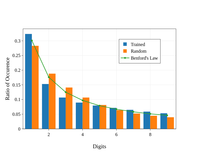
BL defines a probability distribution of a given sample’s significant (leftmost) digit. The leftmost non-zero digit’s occurrence in the observations of a population is log-uniform for several datasets, with 1 occurring the maximum number of times, followed by 2, 3, till 9. According to Benford’s Law (BL) (Benford 1938), the probability for a sample having a significant digit $d$ is given as follows:

$$P_{B}=P(d)=log_{10}(d+\frac{1}{d}),d=1,2,3,...,9$$ (5)

As it is known that RGB images’ pixel values follow BL, we hypothesize that Neural Network weights might also follow BL, for which, we devise a simple metric to measure the similarity of histograms of significant digits of model parameters. We define a simple metric MLH, that measures the correlation between Benford’s Law and histogram of significant digits of a given set.

MLH is based on the Pearson’s Correlation Coefficient (Pearson 1895) is defined as follows:

$$MLH(\theta)=PearsonR(BinCount(\theta),P_{B})$$ (6)

$$BinCount(\theta)=\frac{[f_{0},f_{1},...,f_{9}]}{D_{\theta}}$$ (7)

Here, $BinCount(\theta)$ is the distribution of Significant Digits of network parameter set $\theta$. $P_{B}$ is the distribution defined by BL, $f_{k}$ is is the frequency of significant digit $k$ occurring in $\theta$, $D_{\theta}$ is the dimensionality of $\theta$.

We did not include parameters that are initialized with a constant value, such as Bias and BatchNorm parameters. In our implementation, we multiply all elements in the set by a constant $10^{10}$ so that the resultant elements are greater than zero, and then take the first non-zero digit. This representation is required for a fast vectorized implementation of $BinCount(.)$. Note that multiplying with a constant scalar doesn’t change the distribution of significant digits due to BL’s property of Scale Invariance (Hill 1995b).

This formulation of MLH allows simple implementation and interpretation of the values: The higher the MLH value, the higher the parameters’ match with BL.

Figure 3: AlexNet-like models without dropout trained on CIFAR10. (Left to Right) Training accuracy, validation accuracy and MLH against training iterations. At around 1K iterations, the validation accuracy drops, while the training accuracy reaches 1. It can be clearly observed that the proposed metric MLH follows a similar trajectory to the validation accuracy.

In Fig.2, we compare the Mantissa Distribution of a ResNet152 trained on ImageNet and a randomly initialized ResNet152 (Xavier Normal; Bias and BatchNorm are initialized with a constant). We see that both closely follow BL ($>$0.99 Pearson’s R).

Effect of Initialization on MLH

Enthalpy Information Criterion (EIC) This result points to the possibility that the way Neural Network weights (Xavier Normal) are initialized follow BL closely at the initialization, and after training, the closeness increases even further.

In the this section, we present results on initializing networks with various methods, and show that they achieve high MLH at the end of training regardless of how the network was initialized. To show that a Neural Net’s match with BL is not just due to the virtue of the initialization method. In Fig. 1, we show results of an experiment where we repeatedly train $20$ Shallow Alexnet-like networks each on CIFAR10 for each initialization method, including initializing sub-optimally; we show that the MLH after training is always high regardless of the initial MLH

In the Appendix we explore how MLH varies throughout the depth of pretrained Transformers and ImageNet models, and a peculiar pattern is observed; attempt to find the effect of training data on MLH for various architectures (LSTMs, CNNs, MLPs etc.).

Enthalpy Information Criterion (EIC)

We can think of BL as a prior over significant digits of parameters $\theta$. The choice of BL as a prior is substantiated by the fact that $MLH$ is not an artifact of initialization and therefore possibly contains non-trivial information about a neural network’s initialization. In Eq. 1, $S$ measures the entropy between the distribution over parameters and the prior, however MLH measures distribution of significant digits’ closeness to BL. If we assume that the prior distribution $q(\theta)$ to be approximated by Benford’s Law; $p(\theta)$ by $Bincount(\theta)$, we can see that $S$ is approximated by $MLH(\theta)$. Estimating prior distribution $q(\theta)$ over the parameter set would otherwise be a tedious exercise.

We now define a novel Information Criterion based on MLH:

$$EIC(\theta)=-A_{\theta}-MLH_{\theta}$$ (8)

It can be observed that in Fig. 2, even the randomly initialized network has MLH value over $0.99$. In experiments, we found that the mean MLH of all runs across all steps in RGB Datasets (CIFAR, Stanford Dogs, Oxford Flowers etc.) to be $0.974$, while the minimum and maximum were $0.9462$ and $0.9999$ respectively. We min-max scale MLH to bring it to the range $[0,1]$.

$$EIC_{scaled}(\theta)=-A_{\theta}-\frac{MLH_{\theta}-0.9462}{0.0537}$$ (9)

EIC is related to other information criteria such as Bayesian Information Criteria (BIC) (Schwarz 1978) or Akaike Information Criteria (AIC) (Akaike 1998). However, BIC and AIC both use the number of parameters of the model as a measure of model complexity; unlike EIC, which computes a statistic based on the values of the parameters, hence model complexity can differ for the same model with different parameter values.

We show in the following sections that the property of $S$ to measure the risk of overfitting, is demonstrated by MLH and consequently by EIC.

Figure 4: (Red) Test accuracy of models trained using MLH as early stopping. (Blue) Test accuracy of validation proportions used to dictate early stopping. Complements Table 2.

MLH and Validation Accuracy

Method / Metric	Spearman’s R
A	0.214
MLH	0.583
-1 * EIC w/o Scaling	0.292
-1 * EIC w/ Scaling	0.654
-1 * EIC - SR	0.679
GPR(A)	0.418
GPR(MLH)	0.627
GPR(MLH, A)	0.774

Table 1: Correlation between proposed metrics and Validation Accuracy. A is the Training accuracy. GPR($x_{1},x_{2},x_{3},\dots$) refer to GaussianProcessRegressor fitted with $x_{1},x_{2},x_{3},...$ as input features. It can be seen that Min-max scaling drastically increases correlation for EIC, and improves beyond the correlation of MLH only.

For deep learning projects, researchers and practitioners split the available data into at least three sets: Training, Validation, and Test.

Practitioners use the validation set metrics for many purposes, one such use case is deciding when to stop the training i.e. detect overfitting and stopping the training before the model overfits to the train set. This is known as Early Stopping. Early Stopping requires a criterion that can determine the degree of overfitting, usually given by the validation set accuracy (as a proxy for generalization to unseen data).

In this section, we explore whether closeness to BL is related to validation accuracy. To this end, we train 100 shallow AlexNet-like models without dropout on the CIFAR10 dataset, manually split into train (90%) and validation (10%) sets; and collect MLH, validation and train accuracy over the course of training.

In Fig. 3, we randomly select a few training runs and plot their metrics. We observe that MLH and validation accuracy follow a similar trajectory. We make this observation concrete by computing Spearman’s correlation coefficient (spe 2008) between various metrics and validation accuracy. Spearman’s Correlation Coefficient measures the monotonic relationship between two random samples.

In Table 1, we observe a strong correlation between MLH and validation accuracy. The correlation is even higher if we define a quantity that simply sums training accuracy and min-max scaled MLH. This result shows that MLH and training accuracy could be used to estimate validation accuracy. In section MLH and Thermodynamics, we present the motivation behind using both MLH and training accuracy for estimating validation accuracy.

We also fit Gaussian Process Regression (GPR) models from scikit-learn (Pedregosa et al. 2011) on the metrics collected so that it learns a function mapping from either training accuracy or MLH or both to validation accuracy. We observe that the GPR which uses both training accuracy and MLH has the highest correlation with validation accuracy, strongly indicating that MLH contains non-trivial information about the network’s generalization performance.

Similarly, we also run Symbolic Regression using gp-learn to learn a mapping from Training Accuracy and MLH to Validation Accuracy. We obtain a simple program that doesn’t require min-max scaling while achieving higher correlation than Eq. 9.

$$EIC_{sr}(\theta)=-\frac{\log MLH(\theta)}{A(\theta)}$$ (10)

Early Stopping with MLH

In this section, we present a direct application of MLH. In the previous section, we established that MLH is strongly correlated to validation accuracy. We use this result to replace validation set-based criteria for Early Stopping, while using the data saved as additional training data.

Stopping Criterion	Validation Proportion	Mean (TA)	Std (TA)
MLH	0	58.968	1.51
Validation Accuracy	0.0001	53.948	3.48
	0.0004	56.177	2.78
	0.0016	57.407	2.12
	0.0251	58.039	1.80
	0.1	57.903	2.10
	0.2	57.575	1.58
	0.3	56.371	1.96
	0.4	55.538	1.75

Table 2: Mean and Standard deviation of Test Accuracy (TA) for 100 training runs with various validation proportions.

In Early Stopping, the stopping criterion is monitored throughout the training procedure, and if a certain predefined condition involving the criterion is met, the training is stopped. Usually, the criterion used is the accuracy on the validation set.

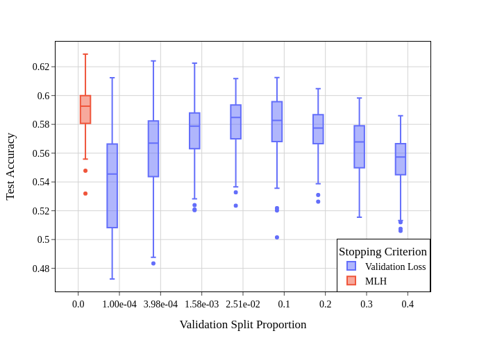
If the data splits are not predefined, as they are in many competitions, the practitioner has to decide on the size of the splits. Early Stopping based on validation set criteria require a validation set to be split off from the training data, which, depending on the size, results in a significant reduction in the amount of available training data. The size of the validation set can also be seen as a hyperparameter. Larger validation sets can result in poorer models due to lower amounts of training data. On the other hand, smaller validation sets can result in inaccurate estimates of generalization performance, and the criteria being unreliable, leading to premature or late stopping. The optimal size of the validation set finds the best trade-off, as observed in Fig. 4. But finding this optimal size of the validation set is non-trivial and requires multiple training runs.

For the experiments in this section, we use the CIFAR10 dataset, and a smaller AlexNet-like model without dropout to make sure the models overfit and hence make our observations concrete. We do a sweep of various validation set sizes and use Validation Accuracy as the Early Stopping metric. For each setting, we train 100 such models for computing confidence intervals. Fig. 4 (Blue) illustrates the validation set size trade-off.

Figure 5: Left: MLH of Energy states at different values of Temperature $T$. Right: MLH of DenseNet121 weights on multiple datasets.

For one set of models, Fig. 4 (Red), we use MLH as the Early Stopping criterion, and include validation data for training. Fig. 4 shows that even if the practitioner knows the optimal validation set size beforehand, the mean test accuracy is significantly lower than when not using a validation set at all.

MLH and Thermodynamics

In the previous sections, we used shallow Alexnet-Like networks that were prone to overfitting. Recent work has shown that larger and deeper neural network architectures are robust to overfitting (Zhang et al. 2017).

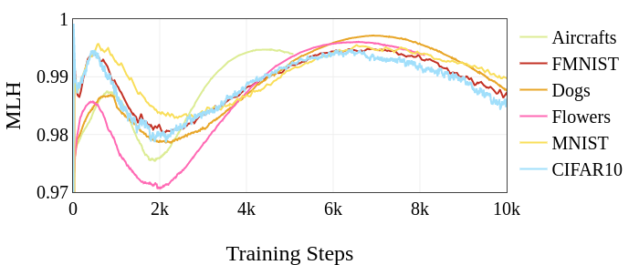
As observed in Fig. 5 (Bottom), when we swap out the smaller AlexNet-like model with a larger DenseNet-121, we observe that the model never clearly overfits. As a result, MLH oscillates periodically; we note this observation on multiple datasets.

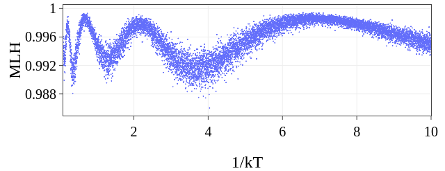
We use this observation to present informal evidence that training NNs can be thought of as a thermodynamic process. We connect this oscillatory pattern of MLH to a contribution by (Shao and Ma 2010) where they find that for systems following Boltzmann-Gibbs statistics, such as an ideal gas in a sealed chamber, their mantissa distribution of energy states of particles oscillates around BL with change in temperature. This is illustrated by Fig. 5 (Top). Here, we run a simulation where we sample a large number of Energy states at a Temperature $T$ with the probability density function for an energy state $E$ from (Shao and Ma 2010),

$$f(E)=\frac{1}{kT}e^{-\frac{E}{kT}}$$ (11)

Here, $k$ is the Boltzmann Constant. We compute MLH of energies at $1/kT=0.1$ to $1/kT=10$ at 10000 equally-spaced values. Fig. 5 (Top) shows how MLH changes as a function of temperature $T$ which strikingly resembles Fig. 5 (Bottom), where we plot 6 models trained on 6 different datasets, and compute MLH of their weights.

Deep Learning	Gas Chamber
Weights	Energy States
Synaptic Connections	Gas Particles
SGD Steps	Reciprocal of Temperature
Train Accuracy	Heat Given
MLH of Weights	Heat Released
Train Accuracy + MLH	Internal Energy

Table 3: Analogies between Deep Learning and Thermodynamics

Furthermore, this motivates us to think about Temperature as an analogous to Gradient Descent iterations, and value of the weights analogous to the Energy states. In Table 3, we list down the analogies drawn between Thermodynamics and Deep Learning. We can think of MLH of weights as the measure of stability, i.e. higher MLH means the distribution of weights is more natural.

Throughout this work, we assumed that MLH is a measure of model complexity, however, explaining why MLH contains this information would possibly also require us to answer why BL even emerges in the first place, which has remained unexplained since the phenomenon was discovered nearly two centuries ago.

Appendix A Appendix

Variation of MLH across Layer Depth

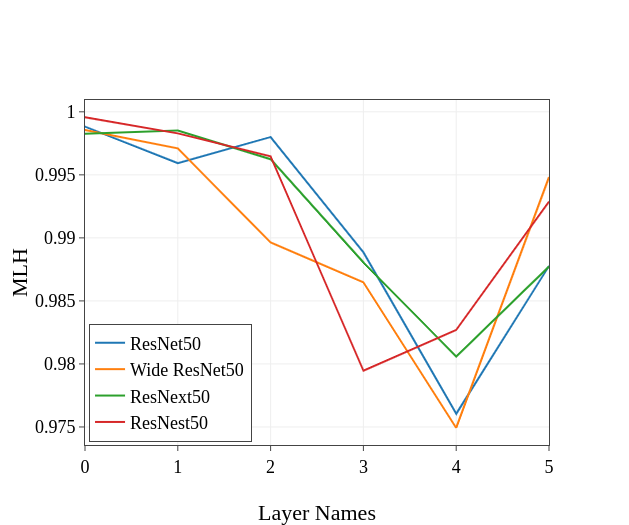
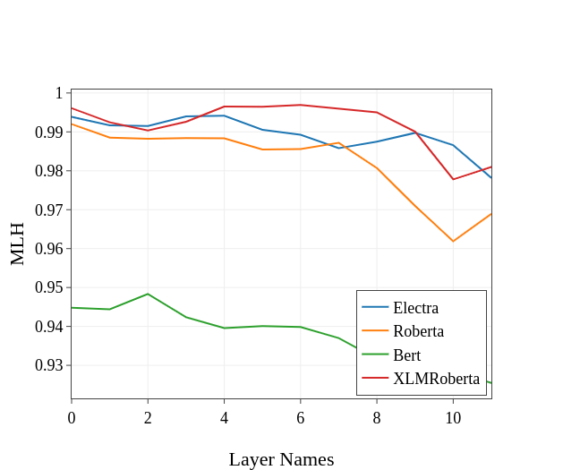
In Fig. 6, we compute MLH for various pre-trained convolutional neural networks and Transformers and plot their layer-wise MLH. We see that generally, the MLH is high at the first layers, decreases gradually, but spikes again at the last layer. A similar trend is observed for Language Models (right).

Figure 6: MLH across different layers of pretrained models.

Effect of Data on MLH

Figure 7: MLH for Datasets and Networks Trained on them.

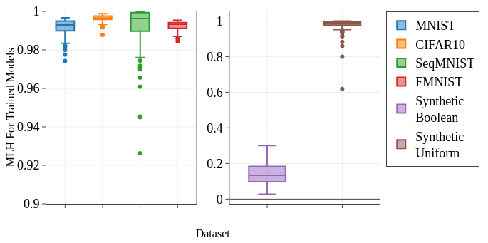
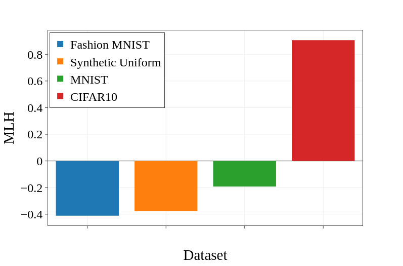
It is well known that RGB Images and their pixel values follow Benford’s Law (Bonettini et al. 2020). We investigate whether the data distribution affects the Network Weights, causing them to match Benford’s Law.

We investigate CIFAR10 (Krizhevsky et al. 2009), MNIST (LeCun and Cortes 2010), FashionMNIST (Xiao, Rasul, and Vollgraf 2017), Sequential MNIST (SeqMNIST) (Goodfellow et al. 2013), two Synthetically Generated Datasets, and 100 Models trained on each of these datasets. We train a small LeNet-inspired network for MNIST and FashionMNIST, DenseNet121 for CIFAR10, LSTM (Hochreiter and Schmidhuber 1997a) for SeqMNIST, and MLP for Synthetic Datasets.

For Synthetic-Boolean Dataset, We generate a random boolean function taking the $argmax$ over a randomly initialized Network with 64 boolean input features. Since the inputs are boolean, i.e., Base 2, Benford’s Law for Base 2 is 1 (Hill 1995a).

For Synthetic-Uniform Dataset, we do the same as above, but the inputs are drawn uniformly from the range $[0,1]$.

Since the Scale Invariance Property of BL holds, we only divide by 255 for Image Datasets and do not normalize this experiment’s features.

As Observed in Figure7, CIFAR10 has positive MLH, and others have Negative MLH, whereas all of the models except for the ones trained on Synthetic-Boolean have $>$0.9 median MLH. Models trained on Synthetic-Boolean have a low but positive median MLH of about 0.2. We believe that MLH of the network is more related to feature variance than MLH of the Data.

Preprocessing of Data

For all experiments, we only divide by the maximum magnitude across features rather than normalizing them. This was to preserve the Scale Invariance Property of Benford’s Law.

Model Architectures

For all experiments in the paper, we use the following architectures and their respective datasets.

Dataset	Architecture
MNIST	LeNet
FashionMNIST	LeNet
CIFAR10	DenseNet-121
SequentialMNIST	LSTM
Synthetic-Uniform	MLP
Synthetic-Boolean	MLP
Oxford-Flowers	DenseNet-121
Stanford-Dogs	DenseNet-121
Aircrafts	DenseNet-121

Table 4: Model architectures used for training on corresponding datasets.

The details of the models that have been used for the experiments are given below:

• LeNet (LeCun et al. 1998) architecture is a simple network with two(2) blocks of Strided Convolution-LeakyReLU Network followed by a fully-connected classification layer.

• DenseNet-121 (Huang et al. 2017) implementation is borrowed from this GitHub repository.

• LSTM is a simple 2-layered RNN with Long-Short Term Memory (Hochreiter and Schmidhuber 1997b) followed by a fully-connected layer for classification.

• MLP is a 2 fully-connected network with Classification (Softmax) and Regression (Linear) output layers for Synthetic-Boolean and Synthetic Uniform Datasets.

Hyperparameters

Unless stated otherwise, all of the experiments use PyTorch’s implementation of Adam (Kingma and Ba 2014), and PyTorch Lightning’s (Falcon 2019) default values except the following wherever applicable.

Parameter	Value
Learning Rate	3e-3
Early Stopping Patience	15
Validation Frequency	0.33
Batch Size	64

Table 5: Hyperparameters used during training

Data Splits

For the datasets other than synthetically generated, we provide the Train/Validation/Test sets. All of them are randomly split unless PyTorch has Train/Test splits.

Dataset	Train	Validation	Test
MNIST	45000	5000	10000
FashionMNIST	45000	5000	10000
CIFAR10	45000	5000	10000
SequentialMNIST	45000	5000	10000
Synthetic-Boolean	6000	2000	2000
Synthetic-Uniform	6000	2000	2000
Oxford-Flowers	6149	2040	0
Stanford-Dogs	12000	8580	0
Aircrafts	6667	3333	0

Table 6: Train, Validation and Test set splits for Datasets used.

Synthetic Data Generation

We use synthetic data set for training a regression and a classification model. The synthetic data is generated using a single layered neural network that is randomly initialized. We describe the process of the generation process below. Both the data sets have an input vector length of 64 and these input vectors are also drawn randomly from Uniform $[0,1]$ and Bernoulli for Synthetic-Uniform and Synthetic-Boolean respectively. We generate 10000 pairs of input-output. These are split in the ratio 60:20:20 for Train, Validation and Test sets respectively.

Regression data set

$x_{i}\in\mathbf{R}^{64}$ is an input vector sampled from $Uniform[0,1]$. The target label $y_{i}\in\mathbf{R}$ is obtained by feeding $x_{i}$ as input to a randomly initialized single layered linear kernel with one output unit, $f_{\theta}$.

$$y_{i}=f_{\theta}(x_{i}),x_{i}\in Uniform[0,1]$$ (12)

Classification data set

$x_{i}\in\mathbf{R}^{64}$ is an input vector sampled from $Bernoulli[0,1]$. The target label $y_{i}\in\mathbf{R}$ is obtained by feeding $x_{i}$ as input to a randomly initialized single layered linear kernel with two output units and argmax-ed over the output vector.

$$y_{i}=argmax[f_{\theta}(x_{i})],x_{i}\in Bernoulli[0,1]$$ (13)

benford = np.array([30.1, 17.6, 12.5, 9.7,
                    7.9, 6.7, 5.8, 5.1, 4.6]
            ) / 100

def mlh(bin_percent):
    return scipy.stats.pearsonr(
                benford,
                bin_percent[1:]
    )[0]

def bincount(tensor):
    counts = torch.zeros(10)
    for i in range(10):
        counts[i] = torch.count_nonzero(
            tensor == i
        )
    return counts

@torch.no_grad()
def bin_percent(tensor):
    tensor = tensor.abs() * 1e10
    long_tensor = torch.log10(tensor).long()
    tensor = tensor // 10 ** long_tensor
    tensor = bincount(tensor.long())
    return tensor / tensor.sum()

Figure 8: PyTorch code for computing MLH

PyTorch Code for Computing MLH

In the code provided in Fig. 8, the vector $benford$ is the distribution defined by Benford’s Law, $bin\_percent$ is a function that takes a tensor as input and returns the distribution of digits in it. $bincount$ is a function that takes a flattened tensor of integers $\in[0,9]$ and returns a vector of frequencies. MLH is the function to compute the proposed MLH score.

References

- spe (2008) 2008. Spearman Rank Correlation Coefficient, 502–505. New York, NY: Springer New York. ISBN 978-0-387-32833-1.
- Acebo and Sbert (2005) Acebo, E.; and Sbert, M. 2005. Benford’s law for natural and synthetic images. In Proceedings of the First Eurographics conference on Computational Aesthetics in Graphics, Visualization and Imaging, 169–176.
- Akaike (1998) Akaike, H. 1998. Information Theory and an Extension of the Maximum Likelihood Principle, 199–213. New York, NY: Springer New York. ISBN 978-1-4612-1694-0.
- Alemi and Fischer (2018) Alemi, A. A.; and Fischer, I. 2018. TherML: Thermodynamics of Machine Learning. arXiv:1807.04162.
- Benford (1938) Benford, F. 1938. The Law of Anomalous Numbers. Proceedings of the American Philosophical Society, 78(4): 551–572.
- Bonettini et al. (2020) Bonettini, N.; Bestagini, P.; Milani, S.; and Tubaro, S. 2020. On the use of Benford’s law to detect GAN-generated images. arXiv preprint arXiv:2004.07682.
- Burnham and Anderson (2003) Burnham, K.; and Anderson, D. R. 2003. Model selection and multimodel inference : a practical information-theoretic approach. Journal of Wildlife Management, 67: 655.
- Falcon (2019) Falcon, W. 2019. PyTorch Lightning. GitHub. Note: https://github.com/PyTorchLightning/pytorch-lightning, 3.
- Friston (2010) Friston, K. 2010. The free-energy principle: a unified brain theory? Nature reviews neuroscience, 11(2): 127–138.
- Gao and Chaudhari (2020) Gao, Y.; and Chaudhari, P. 2020. A Free-Energy Principle for Representation Learning. In III, H. D.; and Singh, A., eds., Proceedings of the 37th International Conference on Machine Learning, volume 119 of Proceedings of Machine Learning Research, 3367–3376. PMLR.
- Goodfellow et al. (2013) Goodfellow, I. J.; Mirza, M.; Xiao, D.; Courville, A.; and Bengio, Y. 2013. An empirical investigation of catastrophic forgetting in gradient-based neural networks. arXiv preprint arXiv:1312.6211.
- Hill (1995a) Hill, T. P. 1995a. Base-Invariance Implies Benford’s Law. Proceedings of the American Mathematical Society, 123(3): 887–895.
- Hill (1995b) Hill, T. P. 1995b. Base-invariance implies Benford’s law. Proceedings of the American Mathematical Society, 123(3): 887–895.
- Hochreiter and Schmidhuber (1997a) Hochreiter, S.; and Schmidhuber, J. 1997a. Long short-term memory. Neural computation, 9(8): 1735–1780.
- Hochreiter and Schmidhuber (1997b) Hochreiter, S.; and Schmidhuber, J. 1997b. Long Short-Term Memory. Neural Computation, 9(8): 1735–1780.
- Huang et al. (2017) Huang, G.; Liu, Z.; Van Der Maaten, L.; and Weinberger, K. Q. 2017. Densely connected convolutional networks. In Proceedings of the IEEE conference on computer vision and pattern recognition, 4700–4708.
- Jolion (2001) Jolion, J.-M. 2001. Images and Benford’s law. Journal of Mathematical Imaging and Vision, 14(1): 73–81.
- Kingma and Ba (2014) Kingma, D. P.; and Ba, J. 2014. Adam: A method for stochastic optimization. arXiv preprint arXiv:1412.6980.
- Krizhevsky et al. (2009) Krizhevsky, A.; et al. 2009. Learning multiple layers of features from tiny images.
- LeCun et al. (1998) LeCun, Y.; Bottou, L.; Bengio, Y.; and Haffner, P. 1998. Gradient-based learning applied to document recognition. Proceedings of the IEEE, 86(11): 2278–2324.
- LeCun and Cortes (2010) LeCun, Y.; and Cortes, C. 2010. MNIST handwritten digit database.
- Pearson (1895) Pearson, K. 1895. VII. Note on regression and inheritance in the case of two parents. proceedings of the royal society of London, 58(347-352): 240–242.
- Pedregosa et al. (2011) Pedregosa, F.; Varoquaux, G.; Gramfort, A.; Michel, V.; Thirion, B.; Grisel, O.; Blondel, M.; Prettenhofer, P.; Weiss, R.; Dubourg, V.; Vanderplas, J.; Passos, A.; Cournapeau, D.; Brucher, M.; Perrot, M.; and Duchesnay, E. 2011. Scikit-learn: Machine Learning in Python. Journal of Machine Learning Research, 12: 2825–2830.
- Sambridge, Tkalčić, and Jackson (2010) Sambridge, M.; Tkalčić, H.; and Jackson, A. 2010. Benford’s law in the natural sciences. Geophysical research letters, 37(22).
- Schwarz (1978) Schwarz, G. 1978. Estimating the Dimension of a Model. The Annals of Statistics, 6(2): 461 – 464.
- Shao and Ma (2010) Shao, L.; and Ma, B.-Q. 2010. The significant digit law in statistical physics. Physica A: Statistical Mechanics and its Applications, 389: 3109–3116.
- Xiao, Rasul, and Vollgraf (2017) Xiao, H.; Rasul, K.; and Vollgraf, R. 2017. Fashion-mnist: a novel image dataset for benchmarking machine learning algorithms. arXiv preprint arXiv:1708.07747.
- Zhang et al. (2017) Zhang, C.; Bengio, S.; Hardt, M.; Recht, B.; and Vinyals, O. 2017. Understanding deep learning requires rethinking generalization.