Online Bin Packing with Predictions

Online Bin Packing with Predictions

Abstract

Bin packing is a classic optimization problem with a wide range of applications from load balancing in networks to supply chain management. In this work we study the online variant of the problem, in which a sequence of items of various sizes must be placed into a minimum number of bins of uniform capacity. The online algorithm is enhanced with a (potentially erroneous) prediction concerning the frequency of item sizes in the sequence. We design and analyze online algorithms with efficient tradeoffs between consistency (i.e., the competitive ratio assuming no prediction error) and robustness (i.e., the competitive ratio under adversarial error), and whose performance degrades gently as a function of the prediction error. This is the first theoretical study of online bin packing in the realistic setting of erroneous predictions, as well as the first experimental study in the setting in which the input is generated according to both static and evolving distributions. Previous work on this problem has only addressed the extreme cases with respect to the prediction error, has relied on overly powerful and error-free prediction oracles, and has focused on experimental evaluation based on static input distributions.

1 Introduction

Bin packing is a classic optimization problem and one of the original NP-hard problems. Given a set of items, each with a (positive) size, and a a bin capacity, the objective is to assign the items to the minimum number of bins so that the sum of item sizes in each bin does not exceed the bin capacity. Bin packing is instrumental in modeling resource allocation problems such as load balancing and scheduling [CGJ96], and has many applications in supply chain management such as capacity planning in logistics and cutting stock. Efficient algorithms for the problem have been proposed within AI [Kor02, Kor03, FK07, SK13].

In this work we focus on the online variant of bin packing, in which the set of items is not known in advance, but is rather revealed in the form of a sequence. Upon the arrival of a new item, the online algorithm must either place it into one of the currently open bins, as long as this action does not violate the bin’s capacity, or into a new bin. The online model has several applications related to dynamic resource management such as virtual machine placement for server consolidation [SXCL13, WMZ11] and memory allocation in data centers [BBV11].

We rely on the standard framework of competitive analysis for evaluating the performance of the online algorithms. In fact, as stated in [CGJ96], bin packing has served as an early proving ground for this type of analysis, in the broader context of online computation. The competitive ratio of an online algorithm is the worst-case ratio of the algorithm’s cost (total number of opened bins) over the optimal offline cost (optimal number of opened bins given knowledge of all items). For bin packing, in particular, the standard performance metric is the asymptotic competitive ratio, in which the optimal offline cost is unbounded (i.e., the sequence is arbitrarily long) [CGJ96].

While the standard online framework assumes that the algorithm has no information on the input sequence, a recently emerged, and very active direction in machine learning seeks to leverage predictions on the input. More precisely, the algorithm has access to some machine-learned information on the input; this information is, in general, erroneous, namely there is a prediction error $\eta$ associated with it. The objective is to design algorithms whose competitive ratio degrades gently as the prediction error increases. Following [LV18], we refer to the competitive ratio of an algorithm with error-free prediction as the consistency of the algorithm, and to the competitive ratio with adversarial prediction as its robustness. Several online optimization problems have been studied in this setting, including caching [LV18, Roh20], ski rental and non-clairvoyant scheduling [PSK18, WZ20], makespan scheduling [LLMV20], rent-or-buy problems [Ban20, AGP20, GP19], secretary and matching problems [AGKK20, LMRX20], and metrical task systems [ACE⁺20]. See also the survey [MV20].

1.1 Contribution

We give the first theoretical and experimental study of online bin packing with machine-learned predictions. Previous work on this problem has either assumed ideal and error-free predictions (given from a very powerful oracle), or only considered tradeoffs between consistency and robustness (see the discussion in Section 1.2). In contrast, our algorithms exploit natural, and PAC-learnable predictions concerning the frequency at which item sizes occur in the input, and our analysis incorporates the prediction error into the performance guarantee. As in other works on this problem, we assume a discrete model in which item sizes are integers in $[1,k]$, for some constant $k$ (see Section 2). This assumption is not indispensable, and in Section 5.2 we extend to items with fractional sizes.

We first present and analyze ProfilePacking, which is an algorithm of optimal consistency, and is also efficient if the prediction error is small. As the error grows, this algorithm may not be robust; we show, however, that this is an unavoidable price that any optimally-consistent algorithm with frequency predictions must pay. We thus design and analyze a class of hybrid algorithms that combine ProfilePacking and any one of the known robust online algorithms, and which offer a more balanced tradeoff between robustness and consistency. These algorithms are suited for the usual setting of inputs generated from an unknown, but fixed distribution. We present a natural heuristic that updates the predictions based on previously served items, and which is better suited for inputs generated from distributions that change over time (e.g., in the case of evolving data [GBEB17]).

We perform extensive experiments on our algorithms. Specifically, we evaluate them on a variety of publicly available benchmarks, such as the BPPLIB benchmarks [DIM], but also on distributions studied in the context of offline bin packing, such as the Weibull distribution [CCO12]. The results show that our algorithms outperform the known efficient algorithms without any predictions.

In terms of techniques, we rely on the concept of a profile set, which serves as an approximation of the items that are expected to appear in the sequence, given the prediction. This is a natural concept that may be further applicable in other online packing problems, such as multi-dimensional packing [CKPT17] and vector packing [ACKS13]. It is worth pointing out that our theoretical analysis is tied to frequency prediction with errors, and treats items “collectively”. In contrast, almost all known online bin packing algorithms are analyzed using a weighting technique [CGJ96], which treats each bin “individually”, and independently from the others (by assigning weights to items, and independently comparing a bin’s weight in the online algorithm and the offline optimal solution).

1.2 Related work

Online bin packing has a long history of study. Simple algorithms such as FirstFit (which places an item into the first bin of sufficient space, and opens a new bin if required), and BestFit (which works similarly, except that it places the item into the bin of minimum available capacity which can still fit the item) are 1.7-competitive [JDU⁺74]. Improving upon this performance requires more sophisticated algorithms, and many such have been proposed in the literature. The currently best upper bound on the competitive ratio is 1.57829 [BBD⁺18], whereas the best known lower bound is 1.54037 [BBG12]. The results above apply to the standard model in which there is no prediction on the input. Other studies include sequential [GLO10] and stochastic settings [GR20].

The problem has also been studied under the advice complexity model [BKLL16, Mik16, ADK⁺18], in which the online algorithm has access to some error-free information on the input called advice, and the objective is to quantify the tradeoffs between the competitive ratio of the algorithm and the size of the advice (in terms of bits). It should be emphasized that such studies are only of theoretical interest, not only because the advice is assumed to have no errors, but also because it may encode any information, with no learnability considerations (i.e., it may be provided by an omnipotent oracle that knows the optimal solution).

Online bin packing was recently studied under an extension of the advice complexity model, in which the advice may be untrusted [ADJ⁺20]. Here, the algorithm’s performance is evaluated only at the extreme cases in which the advice is either error-free, or adversarially generated, namely with respect to its consistency and its robustness, respectively. The objective is to find Pareto-efficient algorithms with respect to these two metrics, as function of the advice size. However, this model is not concerned with the performance of the algorithm on typical cases in which the prediction does not fall in one of the two above extremes, does not incorporate the prediction error into the analysis, and does not consider the learnability of advice. In particular, even with error-free predictions, the algorithm of [ADJ⁺20] has competitive ratio as large as 1.5.

2 Online bin packing: model and predictions

We begin with some preliminary discussions related to our problem. The input to the online algorithm is a sequence $\sigma=a_{1},\ldots,a_{n}$, where $a_{i}$ is the size of the $i$-th item in $\sigma$. We denote by $n$ the length of $\sigma$, and by $\sigma[i,j]$ the subsequence of $\sigma$ that consists of items with indices $i,\ldots,j$ in $\sigma$.

We denote by $k\in\mathbb{Z}^{+}$ the bin capacity. Note that $k$ is independent of $n$, and is thus constant. We assume that the size of each item is an integer in $[1,k]$, where $k$ is the bin capacity. This is a natural assumption on which many efficient algorithms for bin packing rely, e.g., [SK13, FK07, CJK⁺06]. Furthermore, without any restriction on the item sizes,  [Mik16] showed that no online algorithm with advice of size sublinear in the size of the input can have competitive ratio better than 1.17 (even if the advice is error-free). This negative result implies that some restriction on item sizes is required so as to leverage frequency-based predictions. Nevertheless, in Section 5.2 we will extend our algorithms so as to handle fractional items, and we express the performance “loss” due to such items.

Given an online algorithm $A$ (with no predictions), we denote by $A(\sigma)$ its output (packing) on input $\sigma$, and by $|A(\sigma)|$ the number of bins in its output. We denote by $\textsc{Opt}(\sigma)$ the offline optimal algorithm with knowledge of the input sequence. The (asymptotic) competitive ratio of $A$ is defined [CGJ96] as $\lim_{n\to\infty}\sup_{\sigma:|\sigma|=n}|{A(\sigma)}|/{|\textsc{Opt}(\sigma)|}.$

Consider a bin $b$. For the purposes of the analysis, we will often associate $b$ with a specific configuration of items that can be placed into it. We thus say that $b$ is of type $(s_{1},s_{2},\ldots,s_{l},e)$, with $s_{i}\in[1,k],e\in[0,k]$ and $\sum_{j=1}^{l}s_{j}+e=k$, in the sense that the bin can pack $l$ items of sizes $s_{1},\ldots,s_{l}$, with a remaining empty space equal to $e$. We specify that a bin is filled according to type $(s_{1},s_{2},\ldots,s_{l},e)$, if it contains $l$ items of sizes $s_{1},\ldots,s_{l}$, with an empty space $e$. Note that a type induces a partition of $k$ into $l+1$ integers; we call each of the s$l$ elements $s_{1},\ldots,s_{l}$ in the partition a placeholder. We also denote by $\tau_{k}$ the number of all possible bin types. Observe that $\tau_{k}$ depends only on $k$ and not on the length $n$ of the sequence, and is constant, since $k$ is constant.

Consider an input sequence $\sigma$. For any $x\in[1,k]$, let $n_{x,\sigma}$ denote the number of items of size $x$ in $\sigma$. We define the frequency of size $x$ in $\sigma$, denoted by $f_{x,\sigma}$, to be equal to $n_{x,\sigma}/n$, hence $f_{x,\sigma}\in[0,1]$. Our algorithms will use these frequencies as predictions. Namely, for every $x\in[1,k]$, there is a predicted value of the frequency of size $x$ in $\sigma$, which we denote by $f^{\prime}_{x,\sigma}$. The predictions come with an error, and in general, $f^{\prime}_{x,\sigma}\neq f_{x,\sigma}$. To quantify the prediction error, let $\bm{f_{\sigma}}$ and $\bm{f^{\prime}_{\sigma}}$ denote the frequencies and their predictions in $\sigma$, respectively, as points in the $k$-dimensional space. In line with previous work on online algorithms with predictions, e.g. [PSK18], we can define the error $\eta$ as the $L_{1}$ norm of the distance between $\bm{f_{\sigma}}$ and $\bm{f^{\prime}_{\sigma}}$. It should be emphasized that unlike the ideal predictions in previous work [ADJ⁺20], the item frequencies are PAC-learnable. Namely, for any given $\epsilon>0$ and $\delta\in(0,1]$, a sample of size $\Theta((k+\log(1/\delta))/{\epsilon^{2}})$ is sufficient (and necessary) to learn the frequencies of $k$ item sizes with accuracy $\epsilon$ and error probability $\delta$, assuming the distance measure is the L1-distance (see, e.g., [Can20].)

In general, the error $\eta$ may be bounded by a value $H$, i.e., we have $\eta\leq H$. We can thus make a distinction between $H$-aware and $H$-oblivious algorithms, depending on whether the algorithm knows $H$. Such an upper bound may be estimated e.g., from available data on typical sequences. Note however, that unless otherwise specified, we will assume that the algorithm is $H$-oblivious.

We denote by $A(\sigma,\bm{f^{\prime}_{\sigma}})$ the output of $A$ on input $\sigma$ and predictions $\bm{f^{\prime}}_{\sigma}$. To simplify notation, we will omit $\sigma$ when it is clear from context, i.e., we will use $\bm{f^{\prime}}$ in place of $\bm{f^{\prime}_{\sigma}}$.

3 Profile packing

In this section we present an online algorithm with predictions $\bm{f^{\prime}}$ which we call ProfilePacking. The algorithm uses a parameter $m$, which is a sufficiently large, but constant integer, that will be specified later. The algorithm is based on a the concept of a profile, denoted by $P_{\bm{f^{\prime}}}$, which is defined as a multiset that consists of $\lceil f^{\prime}_{x}m\rceil$ items of size $x$, for all $x\in[1,k]$. One may think of the profile as an “approximation” of the multiset of items that is expected as input, given the predictions $\bm{f^{\prime}}$.

Consider an optimal packing of the items in the profile $P_{\bm{f^{\prime}}}$. Since the size of items in $P_{\bm{f^{\prime}}}$ is bounded by $k$, it is possible to compute the optimal packing in constant time (e.g., using the algorithm of [Kor02]). We will denote by $p_{\bm{f^{\prime}}}$ the number of bins in the optimal packing of all items in the profile. Note that each of these $p_{\bm{f^{\prime}}}$ bins is filled according to a certain type that is specified by the optimal packing of the profile. We will simplify notation and use $P$ and $p$ instead of $P_{\bm{f^{\prime}}}$ and $p_{\bm{f^{\prime}}}$, respectively, when $\bm{f^{\prime}}$ is implied.

We define the actions of ProfilePacking. Prior to serving any items, ProfilePacking opens $p$ empty bins of types that are in accordance with the optimal packing of the profile (so that there are $\lceil f^{\prime}_{x}m\rceil$ placeholders of size $x$ in these empty bins). When an item, say of size $x$, arrives, the algorithm will place it into any placeholder reserved for items of size $x$, provided that such one exists. Otherwise, i.e., if all placeholders for size $x$ are occupied, the algorithm will open another set of $p$ bins, again of types determined by the optimal profile packing. We call each such set of $p$ bins a profile group. Note that the algorithm does not close any bins at any time, that is, any placeholder for an item of size $x$ can be used at any point in time, so long as it is unoccupied.

We require that ProfilePacking opens bins in a lazy manner, that is, the $p$ bins in the profile group are opened virtually, and each bin is counted in the cost of the algorithm only after receiving an item. Last, suppose that for some size $x$, it is $f_{x}>0$, whereas its prediction is $f^{\prime}_{x}=0$. In this case, $x$ is not in the profile set $P$. ProfilePacking packs these special items separately from others, using FirstFit. (See Appendix for pseudocode of all algorithms).

3.1 Analysis of ProfilePacking

We first show that in the ideal setting of error-free prediction, ProfilePacking is near-optimal. We will use this result in the analysis of the algorithm in the realistic setting of erroneous predictions. We denote by $\epsilon$ any fixed constant less than 0.2. We define $m$ to be any constant such that $m\geq 3\tau_{k}k/\epsilon$.

Lemma 1.

For any constant $\epsilon\in(0,0.2]$, and error-free prediction ($\bm{f^{\prime}}=\bm{f}$), ProfilePacking has competitive ratio at most $1+\epsilon$.

Proof.  Let $\epsilon^{\prime}=\epsilon/3$ and note that $m\geq\tau_{k}k/\epsilon^{\prime}$. Given an input sequence $\sigma$, denote by $PP(\sigma,\bm{f^{\prime}})$ the packing output by the algorithm. This output can be seen as consisting of $g$ profile group packings (since each time the algorithm allocates a new set of $p$ bins, a new profile group is generated). Since the input consists of $n$ items, and the profile has at least $m$ items, we have that $g\leq\lceil{n}/{m}\rceil$.

Given an optimal packing $\textsc{Opt}(\sigma)$, we define a new packing, denoted by $N$, that not only packs items in $\sigma$, but also additional items as follows. $N$ contains all (filled) bins of $\textsc{Opt}(\sigma)$, along with their corresponding items. For every bin type in $\textsc{Opt}(\sigma)$, we want that $N$ contains a number of bins of that type that is divisible by $g$. To this end, we add up to $g-1$ filled bins of the same type in $N$.

We can argue that $|N|$ is not much bigger than $|\textsc{Opt}(\sigma)|$. We have that $|N|\leq|\textsc{Opt}(\sigma)|+(g-1)\tau_{k}<|\textsc{Opt}(\sigma)|+n\tau_{k}/m\leq|\textsc{Opt}(\sigma)|(1+\tau_{k}k/m)$ (since $|\textsc{Opt}(\sigma)|\geq\lceil n/k\rceil$). We conclude that $|N|\leq(1+\epsilon^{\prime})|\textsc{Opt}(\sigma)|$.

By construction, $N$ contains $g$ copies of the same bin (i.e., bins that are filled according to the same type). Equivalently, we can say that $N$ consists of $g$ copies of the same packing, and we denote this packing by $\overline{N}$. Let $q=|\overline{N}|$ be the number of bins in this packing. We will show that $p$ is not much bigger than $q$, which is crucial in the proof. The number of items of size $x$ in the packing $\overline{N}$ is at least $\lceil n_{x}/g\rceil$, since $N$ contains at least $n_{x}$ items of size $x$. We also can give the following lower bound on $\lceil n_{x}/g\rceil$:

$$\lceil n_{x}/g\rceil \geq\ n_{x}/\lceil n/m\rceil g\leq\lceil n/m\rceil$$ ()

$$>\ n_{x}m/(n+m) \lceil n/m\rceil<(n+m)/m$$ ()

$$=\ n_{x}(m/n-m^{2}/(n^{2}+mn))$$

$$\geq\ n_{x}m/n-m^{2}/(n+m) n_{x}\leq n$$ ()

$$\geq\ \lceil n_{x}m/n\rceil-1-m^{2}/(n+m)$$

$$>\ \lceil n_{x}m/n\rceil-2. m^{2}<n$$ ()

In other words, for any $x\in[1,k]$, $\overline{N}$ packs each item of size $x$ that appears in the profile set, with the exception of at most one such item. From the statement of ProfilePacking, and its optimal packing of the profile set, we infer that $q+k\geq p$. Note that $q\geq|\textsc{Opt}(\sigma)|/g\geq n/(kg)\geq n/(k\lceil n/m\rceil)>(\lceil n/m\rceil m-m)/(k\lceil n/m\rceil)\geq m/k-m^{2}/kn>m/k-\epsilon^{\prime}\geq\tau_{k}/\epsilon^{\prime}-\epsilon^{\prime}>(\tau_{k}-1)/\epsilon^{\prime}>k/\epsilon^{\prime}$. We thus showed that $q>k/\epsilon^{\prime}$, and the inequality $p\leq q+k$ implies that $p<q(1+\epsilon^{\prime})$. We conclude that the number of bins in each profile group is within a factor $(1+\epsilon^{\prime})$ of the number of bins in $\overline{N}$. Moreover, recall that $PP(\sigma,\bm{f^{\prime}})$ consists of $g$ profile groups, and $N$ consists of $g$ copies of $\overline{N}$. Combining this with previously shown properties, we have that $|PP(\sigma,\bm{f^{\prime}})|\leq g\cdot p<g(1+\epsilon^{\prime})q\leq(1+\epsilon^{\prime})(1+\epsilon^{\prime})|\textsc{Opt}(\sigma)|<(1+3\epsilon^{\prime})|\textsc{Opt}(\sigma)|=(1+\epsilon)|\textsc{Opt}(\sigma)|$. ∎

Next, we analyze the algorithm in the realistic setting of erroneous predictions.

Theorem 2.

For any constant $\epsilon\in(0,0.2]$, and predictions $\bm{f^{\prime}}$ with error $\eta$, ProfilePacking has competitive ratio at most $1+(2+5\epsilon)\eta k+\epsilon$.

Proof.

Let $\bm{f}$ be the frequency vector for the input $\sigma$. Of course, $\bm{f}$ is unknown to the algorithm. In this context, $PP(\sigma,\bm{f})$ is the packing output by ProfilePacking with error-free prediction, and from Lemma 1 we know that $|PP(\sigma,\bm{f})|\leq(1+\epsilon)|\textsc{Opt}(\sigma)|.$ Recall that $P_{\bm{f^{\prime}}}$ denotes the profile set of ProfilePacking on input $\sigma$ with predictions $\bm{f^{\prime}}$, and $p_{\bm{f^{\prime}}}$ denotes the number of bins in the optimal packing of $P_{\bm{f^{\prime}}}$; $P_{\bm{f}}$ and $p_{\bm{f}}$ are defined similarly. We will first relate $p_{\bm{f}}$ and $p_{\bm{f^{\prime}}}$ in terms of the error $\eta$. Note that the multisets $P_{\bm{f}}$ and $P_{\bm{f^{\prime}}}$ differ in at most $\sum_{x=1}^{k}\mu_{x}$ elements, where $\mu_{x}=|\lceil f_{x}m\rceil-\lceil f^{\prime}_{x}m\rceil|$. We call these elements differing. We have $\mu_{x}\leq|(f_{x}-f^{\prime}_{x})m|+1$, hence $\sum_{x=1}^{k}\mu_{x}\leq k+\sum_{x=1}^{k}|(f_{x}-f^{\prime}_{x})m|\leq k+\eta m$. We conclude that the number of bins in the optimal packing of $P_{\bm{f^{\prime}}}$ exceeds the number of bins in the optimal packing of $P_{\bm{f}}$ by at most $k+\eta m$, i.e., $p_{\bm{f^{\prime}}}\leq p_{\bm{f}}+k+\eta m$.

Let $g$ and $g^{\prime}$ denote the number of profile groups in $PP(\sigma,\bm{f})$ and $PP(\sigma,\bm{f^{\prime}})$, respectively. We aim to bound $|PP(\sigma,\bm{f^{\prime}})|$, and to this end we will first show a bound on the number of bins opened by $PP(\sigma,\bm{f^{\prime}})$ in its first $g$ profile groups, then in on the number of bins in its remaining $g^{\prime}-g$ profile groups (if $g^{\prime}\leq g$, there is no such contribution to the total cost). For the first part, the bound follows easily: There are $g$ profile groups, each one consisting of $p_{\bm{f^{\prime}}}$ bins, therefore the number of bins in question is at most $g\cdot p_{\bm{f^{\prime}}}\leq g(p_{\bm{f}}+k+\eta m)$. For the second part, we observe that since ProfilePacking is lazy, any item packed by $PP(\sigma,\bm{f^{\prime}})$ in its last $g^{\prime}-g$ packings has to be a differing element, which implies from the discussion above that $PP(\sigma,\bm{f^{\prime}})$ opens at most $g(k+\eta m)$ bins in its last $g^{\prime}-g$ profile groups. The result follows then from the following inequalities:

$$|PP(\sigma,\bm{f^{\prime}})|$$

$$\leq g(p_{\bm{f}}+k+\eta m)+g(k+\eta m)$$

$$=\ g(p_{\bm{f}}+2k+2\eta m)\$$

$$\leq\ g(p_{\bm{f}}+2\eta m(1+\epsilon)) k\leq\epsilon m$$ ()

$$\leq\ g(p_{\bm{f}}+2\eta p_{\bm{f}}k(1+\epsilon)) p_{\bm{f}}\geq\lceil m/k\rceil$$ ()

$$=g\cdot p_{\bm{f}}(1+2\eta k(1+\epsilon))$$

$$\leq|PP(\sigma,\bm{f})|(1+2\eta k(1+\epsilon))$$

$$\leq(1+\epsilon)(1+2\eta k(1+\epsilon))|\textsc{Opt}(\sigma)| |PP(\sigma,\bm{f})|\leq(1+\epsilon)|\textsc{Opt}(\sigma)|$$ (since )

$$=(1+2\eta k(1+\epsilon)^{2}+\epsilon)|\textsc{Opt}(\sigma)|$$

$$=(1+2\eta k(1+\epsilon^{2}+2\epsilon)+\epsilon)|\textsc{Opt}(\sigma)|$$

$$<(1+\eta k(2+5\epsilon)+\epsilon)|\textsc{Opt}(\sigma)|. \epsilon^{2}<\epsilon/2$$ ()

∎

Theorem 2 shows that ProfilePacking has competitive ratio that is linear in $k$. We can prove that this is an unavoidable price that any online algorithm with frequency-based predictions must pay. Specifically, we show the following negative result.

Theorem 3.

Fix any constant $c<1$. Then for any $\alpha>0$, with $\alpha\leq 1/k$, any algorithm with frequency predictions that is $(1+\alpha)$-consistent has robustness at least $(1-c)k/2$.

Proof.

Suppose that the prediction indicates that in the input sequence $\sigma$, half of the items have size $1$ and the other half have size $k-1$, i.e., we have $f^{\prime}_{x,\sigma}=1/2$, if $x\in\{1,k-1\}$, and $f^{\prime}_{x,\sigma}=0$, otherwise. Define $\sigma_{1}$ as the sequence that consists of $n$ items of size $1$ followed by $n$ items of size $k-1$, and $\sigma_{2}$ as the sequence that consists of $n$ items of size $1$ followed by $n$ items of size $1$. For simplicity, assume $n$ is divisible by $k$. Suppose first that the input is $\sigma_{1}$, then the prediction is error-free. Moreover, $\textsc{Opt}(\sigma_{1})=n$ and hence for an algorithm A to be $(1+\alpha)$-consistent, no more than $\alpha n+o(n)$ bins should receive more than one item of size $1$. This implies that A opens at least $(1-k\alpha)n-o(n)$ bins for the first $n$ items. Next, suppose that the input is $\sigma_{2}$. We have ${f}_{1,\sigma_{2}}=1$ and ${f}_{k-1,\sigma_{2}}=0$, and consequently the error is $\eta=1$. Moreover, $\textsc{Opt}(\sigma_{2})=2n/k$, while the cost of A is at least $(1-k\alpha)n-o(n)$. The competitive ratio of A is at least $((1-k\alpha)n-o(n))/(2n/k)$. Given that $\alpha\leq c/k$, A has robustness at least $(1-c)k/2$. ∎

We conclude that the robustness of ProfilePacking is close-to-optimal and no $(1+\epsilon)$-consistent algorithm can do asymptotically better. It is possible, however, to obtain more general tradeoffs between consistency and robustness, as we discuss in the next section.

Time complexity.

We bound the overall time complexity of ProfilePacking for serving a sequence of $n$ items as a function of $n,k$, and $m$. The initial phase of the algorithm runs in time independent of $n$. Therefore, the asymptotic time complexity is dominated by the time required to pack the items into the appropriate bins.

For any $x\in[1,k]$, one can maintain $N_{x}$ and $E_{x}$ (subsets of $\mathit{NonEmpty}$ and $\mathit{Empty}$ that contain $x$) using a hash table, where keys are bin-types and values are the number of bins of a given type. As such, for any $i\in[1,n]$, we can pack $\sigma[i]$ in $N_{x}$ or $E_{x}$ (assuming that they are not empty) in $O(1)$ amortized time. If both $N_{x}$ and $E_{x}$ are empty, the algorithm opens a new profile group. This requires updating $k$ hash tables (for any $E_{x}$ for $x\in[1,k]$), where we add $O(m)$ new bin-types to each hash table. Consequently, the time complexity of adding a new profile group is $O(mk)$.

In the ideal case $\eta=0$, $O(n/m)$ profile groups are opened and the time complexity of adding profile groups is $O(kn)$, which also defines the time complexity of the algorithm. If $\eta>0$, there are up to $n$ profile groups, which results in a worst-case time complexity of $O(kmn)$ for adding profile groups. Note that when $\eta>0$, up to $\Theta(n)$ items are special and served using FirstFit. The complexity of packing these items (i.e., the complexity of FirstFit) is $O(kn)$ which is dominated by $O(kmn)$, namely the time of adding profile groups. In conclusion, the worst-case time complexity of ProfilePacking is $O(kmn)$. Note that each item is served in amortized time $O(km)$, which is constant since $k$ and $m$ are constants.

We emphasize that our complexity bounds apply in the worst-case, and are rather pessimistic. In practice, the algorithms run much faster; see Section 6.4.

4 A hybrid algorithm

In this section we obtain online bin packing algorithms of improved robustness. The main idea is to let ProfilePacking serve only certain items, whereas the remaining ones are served by an online algorithm $A$ that is robust. In particular, let $A$ denote any algorithm of competitive ratio $c_{A}$, in the standard online model in which there is no prediction. We will define a class of algorithms based on a parameter $\lambda\in[0,1]$ which we denote by Hybrid($\lambda$). Let $a,b\in\mathbb{N}^{+}$ be such that $\lambda=a/(a+b)$. We require that the parameter $m$ in the statement of ProfilePacking is a sufficiently large constant, namely $m\geq 5\tau_{k}\max\{k,a+b\}/\epsilon$.

Upon arrival of an item of size $x\in[1,k]$, Hybrid($\lambda$) marks it as either an item to be served by ProfilePacking, or as an item to be served by $A$; we call such an item a PP-item or an $A$-item, in accordance to this action. Moreover, for every $x\in[1,k]$, Hybrid($\lambda$) maintains two counters: ${\tt count}(x)$, which is the number of items of size $x$ that have been served so far, and ${\tt ppcount}(x)$, which is the number of PP-items of size $x$ that have been served so far.

We describe the actions of Hybrid($\lambda$). Suppose that an item of size $x$ arrives. If there is an empty placeholder of size $x$ in a non-empty bin, then the item is assigned to that bin (and to the corresponding placeholder), and declared PP-item. Otherwise, there are two possibilities: If ${\tt ppcount}(x)$ $\leq\lambda\cdot$ ${\tt count}(x)$, then it is served using ProfilePacking and is declared PP-item. If ${\tt ppcount}(x)$ $>\lambda\cdot$ ${\tt count}(x)$, then it is served using $A$ and declared $A$-item.

Note that in Hybrid($\lambda$), $A$ and ProfilePacking maintain their own bin space, so when serving according to one of these algorithms, only the bins opened by the corresponding algorithm are considered. Thus, we can partition the bins used by Hybrid($\lambda$) into PP-bins and $A$-bins.

Theorem 4.

For any $\epsilon\in(0,0.2]$ and $\lambda\in[0,1]$, Hybrid($\lambda$) has competitive ratio $(1+\epsilon)((1+(2+5\epsilon)\eta k+\epsilon)\lambda+c_{A}(1-\lambda))$, where $c_{A}$ is the competitive ratio of $A$.

Proof 1.

We define two partitions of the multiset of items in $\sigma$. The first partition is $S_{PP}\cup S_{A}$, where $S_{PP}$ and $S_{A}$ are the PP-items and A-items of Hybrid($\lambda$), respectively. The second partition is $S^{\prime}_{PP}\cup S^{\prime}_{A}$, where $S^{\prime}_{PP}$ and $S^{\prime}_{A}$ are defined such that for any $x\in[1,k]$ there are $\lfloor\lambda n_{x}\rfloor$ items of size $x$ in $S^{\prime}_{PP}$ and $n_{x}-\lfloor\lambda n_{x}\rfloor$ items of size $x$ in $S^{\prime}_{A}$. Given $\textsc{Opt}(\sigma)$, we will define a new packing $N$, such that every bin in $N$ contains only items in $S^{\prime}_{PP}$ or only items in $S^{\prime}_{A}$. Let $N_{PP}$ and $N_{A}$ denote the set of bins in $N$ that include items in $S^{\prime}_{PP}$ and in $S^{\prime}_{A}$, respectively. Similarly, let $B_{PP}$ and $B_{A}$ denote the set of bins in the packing of Hybrid($\lambda$) that contain only PP-items (PP-bins) and A-items (A-bins), respectively. We prove the following bounds for $N$, $B_{PP}$ and $B_{A}$:

• $|N|\leq(1+\epsilon)|\textsc{Opt}(\sigma)|$.

• $|B_{PP}|\leq(1+(2+5\epsilon)\eta k+\epsilon)|N_{PP}|$.

• $|B_{A}|\leq c_{A}|N_{A}|$.

To prove the above bounds, We first explain how to derive $N$ from $\textsc{Opt}(\sigma)$. This is done in a way that $N$ contains the filled bins of $\textsc{Opt}(\sigma)$ and up to $(a+b)\tau_{k}$ additional filled bins so as to guarantee that the number of bins of each given type in $N$ is divisible by $a+b$. Given that $m\geq 5\tau_{k}\max\{k,a+b\}/\epsilon$, we can use an argument similar to the proof of Lemma 1 to show $|N|\leq(1+\epsilon)|\textsc{Opt}(\sigma)|$. Since the number of bins of each type in $N$ is divisible by $a+b$, we can partition $N$ into $N_{PP}$ and $N_{A}$ so that $|N_{PP}|\leq a(1+\epsilon)|\textsc{Opt}(\sigma)|/(a+b)$ and $|N_{A}|\leq b(1+\epsilon)|\textsc{Opt}(\sigma)|/(a+b)$. That is, $|N_{PP}|\leq\lambda(1+\epsilon)|\textsc{Opt}(\sigma)|$ and $N_{A}\leq(1-\lambda)(1+\epsilon)|\textsc{Opt}(\sigma)|$. Note that $N$ not only packs items in $\sigma$, but also additional items in the added bins. That implies that all items $S^{\prime}_{PP}$ are packed in $N_{PP}$ and all items in $S^{\prime}_{A}$ are packed in $N_{A}$, and hence (i) follows.

To prove (ii) and (iii), we note that $S_{A}\subseteq S^{\prime}_{A}$ which implies $S^{\prime}_{PP}\subseteq S_{PP}$. This is because the algorithm declares an item of size $x$ as A-item only if ${\tt ppcount}(x)$ $>\lambda$ ${\tt count}(x)$. Hence, at any given time during the execution of Hybrid($\lambda$), the number of A-items of size $x$ is no more than a fraction $(1-\lambda)$ of ${\tt count}(x)$.

Next we will show property (ii). First, note that $|B_{PP}|=|PP(\sigma_{PP},\bm{f^{\prime}})|$, where $\sigma_{PP}$ is the subsequence of $\sigma$ formed by the $PP$-items, and $PP$ abbreviates the output of ProfilePacking. Consider a sequence $\sigma^{\prime}_{PP}$ obtained by removing, for every $x\in[1,k]$, the last $d_{x}$ items of size $x$ from $\sigma_{PP}$, where $d_{x}$ is the number of items of size $x$ in $S_{PP}\setminus S^{\prime}_{PP}$. We show next that $|PP(\sigma_{PP},\bm{f^{\prime}})|=|PP(\sigma^{\prime}_{PP},\bm{f^{\prime}})|$. For any $x$, consider the last PP-item $L_{x}$ of size $x$ for which Hybrid($\lambda$) opens a new bin. At the time $L_{x}$ is packed, ${\tt ppcount}(x)$ $\leq\lambda\cdot$${\tt count}(x)$. Thus, by removing items of size $x$ that appear after $L_{x}$ in $\sigma_{PP}$, the remaining items form a subsequence of $\sigma^{\prime}_{PP}$, and the number of bins does not decrease. That implies that $|PP(\sigma_{PP},\bm{f^{\prime}})|=|PP(\sigma^{\prime}_{PP},\bm{f^{\prime}})|$. From Theorem 2, $|B_{PP}|=|PP(\sigma_{PP},\bm{f^{\prime}})|=|PP(\sigma^{\prime}_{PP},\bm{f^{\prime}})|\leq(1+(2+5\epsilon)\eta k+\epsilon)|\textsc{Opt}(\sigma^{\prime}_{PP})|\leq(1+(2+5\epsilon)\eta k+\epsilon)|N_{PP}|$.

Last, to show (iii), we note that the number of bins that Hybrid($\lambda$) opens for items in $S_{A}$ is at most $c_{A}|\textsc{Opt}(S_{A})|\leq c_{A}|\textsc{Opt}(S^{\prime}_{A})|\leq c_{A}|N_{A}|$. This is because $S_{A}\subseteq S^{\prime}_{A}$.

Using properties (i)-(iii), we obtain $|{\sc Hybrid}(\sigma,\bm{f^{\prime}})|=\ |B_{PP}|+|B_{A}|\leq\ (1+(2+5\epsilon)\eta k+\epsilon)|N_{PP}|+c_{A}|N_{A}|\leq\ (1+(2+5\epsilon)\eta k+\epsilon)\lambda(1+\epsilon)|\textsc{Opt}(\sigma)|+c_{A}(1-\lambda)(1+\epsilon)|\textsc{Opt}(\sigma)|=(1+\epsilon)((1+(2+5\epsilon)\eta k+\epsilon)\lambda+c_{A}(1-\lambda))|\textsc{Opt}(\sigma)|.$

One can choose $A$ as the algorithm of the best known competitive ratio [BBD⁺18]. However, algorithms such as the one of [BBD⁺18] belong in a class that is tailored to worst-case competitive analysis (namely the class of harmonic-based algorithms) and do not tend to perform well in typical instances [KLO15]. For this reason, simple algorithms such as FirstFit and BestFit are preferred in practice [CGJ96]. We obtain the following corollary.

Corollary 5.

For any $\epsilon\in(0,0.2]$ and $\lambda\in[0,1]$, there is an algorithm with competitive ratio $(1+\epsilon)(1.5783+\lambda((2+5\epsilon)\eta k-0.5783+\epsilon))$. Furthermore, Hybrid($\lambda$) using FirstFit has competitive ratio $(1+\epsilon)(1.7+\lambda((2+5\epsilon)\eta k-0.7+\epsilon))$.

From Theorem 4, it follows that for Hybrid($\lambda$) to be robust, one must chose $\lambda=1/\Omega(k)$, which in turn implies that the consistency is not much better than $c_{A}$. But we can do substantially better if an upper bound on the error $H$ is known. Specifically, let $H$-Aware denote the algorithm which executes Hybrid(1), if $H<(c_{A}-1-\epsilon)/(k(2+5\epsilon))$, and Hybrid(0), otherwise. An equivalent statement is that $H$-Aware executes ProfilePacking if $H<(c_{A}-1-\epsilon)/(k(2+5\epsilon))$, and $A$, otherwise. The following corollary follows directly from Theorem 4 with the observation that as long as $\eta<(c_{A}-1-\epsilon)/(k(2+5\epsilon))$, ProfilePacking has a competitive ratio better than $c_{A}$.

Corollary 6.

For any $\epsilon\in(0,0.2]$, $H$-Aware using algorithm $A$ has competitive ratio $\min\{c_{A},1+(2+5\epsilon)\eta k+\epsilon\}$, where $c_{A}$ is the competitive ratio of $A$. In particular, choosing FirstFit as $A$, $H$-Aware has competitive ratio $\min\{1.7,1+(2+5\epsilon)\eta k+\epsilon\}$.

Time complexity.

A fraction of at least $\lambda$ items of each given size are served using ProfilePacking and a fraction of at most $1-\lambda$ are served using $A$. This implies that the running time of the algorithm is $O(kmn+A(k,n))$, where $A(k,n)$ denotes the running time of $A$. In particular, if $A$ is FirstFit, we have $A(k,n)=O(kn)$ (FirstFit can be implemented by maintaining a pointer for each $x\in[1,k]$ that points to the first bin in the packing with empty space of size at least $x$ and observing that any such pointer is updated at most $n$ times in the course of the algorithm). Thus, the time complexity of Hybrid($\lambda$) is $O(kmn)$. Once again, each item is served in $O(1)$ amortized time.

5 Extensions

5.1 An adaptive heuristic

In all previous algorithms the prediction does not change throughout their execution. While such algorithms can be useful for inputs that are drawn from a fixed distribution, they may not always perform well if the input sequence is generated from distributions that change with time, e.g., when dealing with evolving data streams. We define a heuristic called Adaptive($w$), in which predictions are updated dynamically using a sliding window approach; see e.g. [GBEB17].

Adaptive($w$) uses a parameter $w\in\mathbb{N^{+}}$ as follows. In the initial phase, Adaptive($w$) serves $\sigma[1,w]$ using FirstFit; moreover, at the end of this phase, it computes $\bm{f_{\sigma[1,w]}}$, namely the frequency vector of all sizes in $\sigma[1,w]$. From this point onwards, the algorithm will serve items using ProfilePacking with predictions $\bm{f^{\prime}}$ which are initialized to $\bm{f_{\sigma[1,w]}}$. Specifically, every time Adaptive($w$) encounters item $\sigma[iw]$, for $i\in\mathbb{N}^{+}$, it updates $\bm{f^{\prime}}$ to $\bm{f_{\sigma[(i-1)w+1,iw]}}$.

Time complexity.

The running time of Adaptive($w$) is dominated by computing an optimal profile packing, which can be done in time $O(m^{m+1})$. We note that this is only a crude upper bound, and in practice, algorithms such as the one of Korf [Kor02, Kor03] perform much better in typical instances; moreover, since $m$ is a constant, theoretically this time is $O(1)$. Given that the number of profile groups is $O(n/m)$, Adaptive($w$) runs in time $O(nm^{m})$. If we use FirstFitDecreasing instead of an optimal algorithm (in Line 28), then it takes time $O(m(\log m+k))$ to compute a profile packing (sorting the items in the profile set requires time $O(m\log m)$ and FirstFit requires time $O(mk)$). The overall running time of Adaptive($w$) is thus $O(n(\log m+k)))$ in this alternative. As with all other algorithms, each item is served in $O(1)$ amortized time.

5.2 Handling items with fractional sizes

As stated in Section 2, we assume that each item has integral size in $[1,k]$, where $k$ is the bin capacity. We argue how to extend the algorithms and the analysis so as to handle items with sizes in $[1,k]$ that may be fractional. The main idea is to treat such fractional items as “special”, in the sense that they are not predicted to appear in the sequence. ProfilePacking and Hybrid($\lambda$) will then pack these fractional items separately from all integral ones, using FirstFit.

For the analysis in this setting, we need a measure of “deviation” of the input sequence $\sigma$ (that may contain fractional items) from a sequence of integral sizes. The most natural approach is to define this deviation as the $L_{1}$ distance between $\sigma$, and the sequence in which each item is rounded to the closest integer in $[0,k]$. However, we will show that this definition is very restrictive, in that every online algorithm has consistency far from optimal, even if this deviation is arbitrarily small.

Given an input sequence $\sigma$ which may include items of fractional sizes, we first need to clarify how item frequencies are generated. Let $\lfloor\sigma\rceil$ be derived from $\sigma$ so that each fractional item is replaced with its closest integer. Then we define $\bm{f}$ to be such that for every $x\in\mathbb{Z}^{+}$ with $x\in[1,k]$, we have $f_{x,\sigma}=f_{x,\lfloor\sigma\rceil}$. The prediction vector $\bm{f}^{\prime}$ likewise concerns items of integral size in $[1,k]$, and the error $\eta$ is the $L_{1}$ distance between $\bm{f}^{\prime}$ and $\bm{f}$, as defined above.

Theorem 7.

Let $\lfloor x\rceil$ denote the integer closest to $x$, and define $d(\sigma)=\sum\nolimits_{x\in\sigma}|x-\lfloor x\rceil|$. No online algorithm can have competitive ratio better than 4/3, even if all frequency predictions are error-free (that is, $\eta=0$), and even if $d(\sigma)=\epsilon$, for arbitrarily small $\epsilon>0$.

Proof.

Let $\sigma=\sigma_{1}\sigma_{2}$, where $\sigma_{1}$ consists of $n$ items of size $0.5-\epsilon/(2n)$, and $\sigma_{2}$ consists of $n$ items of size $0.5+\epsilon/(2n)$. For simplicity, we assume that $n$ and $k$ are even integers. Suppose also that $\bm{f^{\prime}}$ is such that $f_{x,\lfloor\sigma\rceil}=1$, if $x=k/2$, and 0, otherwise (i.e., only items of size $k/2$ are predicted to appear in $\sigma$). From the definition of error, it also follows that $\eta=0$, and from the definition of the deviation $d$, we have that $d(\sigma)=\epsilon$.

Let $A$ be any online algorithm, and note that $A(\sigma_{1},{\bm{f}^{\prime}})=cn$, for some $c\geq 1/2$. Given that $\textsc{Opt}(\sigma_{1})=n/2$, the competitive ratio of $A$ is at least $2c$. Out of the $cn$ bins of $A(\sigma_{1},\bm{f^{\prime}})$, $n-cn$ bins must have two items, whereas the remaining $cn-(n-cn)=2cn-n$ bins must have one item. Any of these remaining bins can each accommodate another item from $\sigma_{2}$. Therefore, out of the $n$ items in $\sigma_{2}$, $A$ can pack at most $2cn-n$ such items in the $cn$ bins opened for $\sigma_{1}$, and it must place the remaining $n-(2cn-n)=2n-2cn$ items in separate (new) bins. It follows that $A(\sigma,{\bm{f}^{\prime}})\geq cn+(2n-2cn)=2n-cn$. Given that $\textsc{Opt}(\sigma)=n$, the competitive ratio of A is therefore at least $2-c$. In summary, the competitive ratio of A is $\max\{2c,2-c\}$, which is minimized at $4/3$ for $c=2/3$. ∎

Given the above negative result, a different measure of “deviation” is the ratio between the total size of fractional items in $\sigma$ over the total size of all items in $\sigma$. The following theorem shows that this measure can better capture the performance of the algorithm in the fractional setting.

Theorem 8.

Define $\hat{d}(\sigma)=(\sum_{x\in\sigma,x\neq\lfloor x\rfloor}x)/(\sum_{x\in\sigma}x)$. Let $A$ be any algorithm with frequency predictions that has competitive ratio $c$ if all items have integral size. Then there is an algorithm $A^{\prime}$ that has competitive ratio at most $c+2\hat{d}(\sigma)$ for inputs with fractional sizes.

Proof.

Let $\sigma_{I}$ and $\sigma_{F}$ be the subsequences of $\sigma$ formed by integer and fractional items, respectively. We can write $A(\sigma)=A(\sigma_{I})+FF(\sigma_{F})$, where $FF(\sigma_{F})$ denotes the number of bins opened by FirstFit when serving $\sigma_{F}$. For the number of bins opened for integer items, we have $A(\sigma_{I})\leq A(\sigma)\leq c\cdot\textsc{Opt}(\sigma)$. Let $S(\sigma)$ and $S(\sigma_{F})$ denote the total size of items in $\sigma$ and $\sigma_{F}$, respectively, that is $S(\sigma)=\sum_{x\in\sigma}x$, and $S(\sigma_{F})=\sum_{x\in\sigma,x\neq\lfloor x\rfloor}x$. From definition, we have $\hat{d}(\sigma)=S(\sigma_{F})/S(\sigma)$. Note that $FF(\sigma_{F})\leq 2S(\sigma_{F})/k+1$; this is because any pair of consecutive bins contains items of total size $k/2$ or larger. Therefore, $FF(\sigma_{F})\leq 2\hat{d}(\sigma)S(\sigma)/k+1\leq 2\hat{d}(\sigma)\textsc{Opt}(\sigma)+1$. In summary, we have $A(\sigma)\leq c\cdot\textsc{Opt}(\sigma)+2\hat{d}(\sigma)\textsc{Opt}(\sigma)+1$, therefore the (asymptotic) competitive ratio of $A$ is at most $c+2\hat{d}(\sigma)$. ∎

5.3 VM placement: inputs with large items

As discussed in the Introduction, an important application of online bin packing is Virtual Machine (VM) placement in large data centers. Here, each VM corresponds to an item whose size represents the resource requirement of the VM, and each bin corresponds to a physical machine (i.e., host) of a given capacity $k$. In the context of this application, the consolidation ratio [BB12] is the number of VMs per host, in typical scenarios. Note that the consolidation ratio is typically much smaller than $k$. For example, VMware server virtualization achieves a consolidation ratio of up to 15:1 [VMw], while Intel’s virtualization infrastructure gives a consolidation ratio of up to 20:1 [Ove10]. Let us denote by $r$ the consolidation ratio (but note that this quantity is an integer).

The fact that the consolidation ratio is typically much smaller than $k$ has implications in the analysis of our algorithms. Specifically, we can express the competitive ratio of ProfilePacking and Hybrid($\lambda$) as a function of $r$ instead of $k$, as shown in the following result.

Theorem 9.

Consider an instance of online bin packing with bins of capacity $k$, in which the item sizes are such that at most $r$ items can fit into a bin, for some $r\leq k$. Then, for any constant $\epsilon\in(0,0.2]$, and predictions $\bm{f^{\prime}}$ with error $\eta$, the following hold: (I) ProfilePacking has competitive ratio at most $1+(2+5\epsilon)\eta r+\epsilon$; and (II) for any $\lambda\in[0,1]$, Hybrid($\lambda$) has competitive ratio $(1+\epsilon)((1+(2+5\epsilon)\eta r+\epsilon)\lambda+c_{A}(1-\lambda))$, where $c_{A}$ is the competitive ratio of the algorithm $A$ that is combined with Hybrid($\lambda$).

Proof.

The proof of (I) is identical to that of Theorem 2, except that in the fourth inequality we use the fact that $p_{\bm{f}}\geq\lceil m/r\rceil$ (instead of $p_{\bm{f}}\geq\lceil m/k\rceil$), given that at most $r$ items fit into each bin. Moreover, in all subsequent inequalities in the proof, $k$ is replaced with $r$. The proof of (II) is identical to that of Theorem 4, except that property (ii) in the proof is replaced by $|B_{PP}|\leq(1+(2+5\epsilon)\eta r+\epsilon)|N_{PP}|$, which directly follows from the same arguments and by applying part (I) instead of Theorem 2. ∎

Similarly, we can generalize Theorem 3 and obtain the following impossibility result.

Theorem 10.

Consider an instance of online bin packing with bins of capacity $k$, in which the item sizes are such that at most $r$ items can fit into a bin, for some $r\leq k$. Fix any constant $c<1$. Then for any $\alpha>0$, with $\alpha\leq 1/r$, any algorithm with frequency predictions that is $(1+\alpha)$-consistent has robustness at least $(1-c)r/2$.

Note that in Theorems 9 and 10, the robustness of the algorithms is now a function of $r$, and not a function of $k$, as in Theorems 2 and 4.

6 Experimental evaluation

6.1 Benchmarks

Several benchmarks have been used in previous work on (offline) bin packing (see [CCO12] for a list of related work). These benchmarks typically rely on either uniform or normal distributions. There are two important issues to take into account. First, such simple distributions are often unrealistic and do not capture typical applications of bin packing such as resource allocation [Gen98]. Second, in what concerns online algorithms, simple algorithms such as FirstFit and BestFit are very close to optimal for input sequences generated from uniform distributions [CGJ96] and very often outperform, in practice, many online algorithms of better competitive ratio [KLO15].

We evaluate our algorithms on two types of benchmarks. The first type is based on the Weibull distribution, and was first studied in [CCO12] as a model of several real-world applications of bin packing, e.g., the 2012 ROADEF/EURO Challenge on a data center problem provided by Google and several examination timetabling problems. The Weibull distribution is specified by two parameters: the shape parameter $sh$ and the scale parameter $sc$ (with $sh,sc>0$). The shape parameter defines the spread of item sizes: lower values indicate greater skew towards smaller items. The scale parameter, informally, has the effect of stretching out the probability density. In our experiments, we chose $sh\in[1.0,4.0]$. This is because values outside this range result in trivial sequences with items that are generally too small (hence easy to pack) or too large (for which any online algorithm tends to open a new bin). The scale parameter is not critical, since we scale items to the bin capacity, as discussed later; we thus set $sc=1000$, in accordance with [CCO12].

The second type of benchmarks is generated from the BPPLIB Bin Packing Library [DIM]. This is a collection of bin packing benchmarks used in various works on (offline) algorithms for bin packing. We report experimental results for different benchmarks of the BPPLIB Bin Packing Library [DIM], in particular the benchmarks “GI" [GI16], “Schwerin" [SW97], “Randomly_Generated" [DIM14], “Schoenfield_Hard28" [Sch02] and “Wäscher" [WG96].

6.2 Input generation

We fix the size of the sequence to $n=10^{6}$. We set the bin capacity to $k=100$, and we also scale down each item to the closest integer in $[1,k]$. This choice is relevant for applications such as Virtual Machine placement, as we explained in Section 5.3. We generate two classes of input sequences.

Sequences from a fixed distribution. For Weibull benchmarks, the input sequence consists of items generated independently and uniformly at random, for the shape parameter set to $sh=3.0$. For BPPLIB benchmarks, each item is chosen uniformly and independently at random from the item sizes in one of the benchmark files; this file is also chosen uniformly at random.

Sequences from an evolving distribution.  Here, the distribution of the input sequence changes every 50000 items. Namely, the input sequence is the concatenation of $n/50000$ subsequences. For Weibull benchmarks, each subsequence is a Weibull distribution, whose shape parameter is chosen uniformly at random from $[1.0,4.0]$. For BPPLIB benchmarks, each subsequence is generated by choosing a file uniformly at random, then generating $50000$ items uniformly at random from that specific file.

6.3 Compared algorithms, predictions and error

We evaluate Hybrid($\lambda$) using FirstFit, for $\lambda\in\{0,0.25,0.5,0.75,1\}$. This means that Hybrid(0) is identical to FirstFit, whereas Hybrid(1) is identical to ProfilePacking. We fix the size of the profile set to $m=5000$. To ensure a time-efficient and simplified implementation of ProfilePacking, we use the FirstFitDecreasing algorithm [CGJ96] to compute the profile packing, instead of an optimal algorithm. FirstFitDecreasing first sorts items in the non-increasing order of their sizes and then applies the FirstFit algorithm to pack the sorted sequence. Using FirstFitDecreasing helps reduce the time complexity, in particular with regards to Adaptive($w$), which must compute a new profile packing every time it updates the frequency prediction. The experimental results only improve by using an optimal profile packing instead of FirstFitDecreasing.

We evaluate Hybrid($\lambda$) on fixed distributions, since it is tailored to this type of input. We generate the frequency predictions to Hybrid($\lambda$) as follows: For a parameter $b\in\mathbb{N}^{+}$, we define the predictions $\bm{f^{\prime}}$ as $\bm{f_{\sigma[1,b]}}$. In words, we use a prefix of size $b$ of the input $\sigma$ so as to estimate the frequencies of item sizes in $\sigma$. In our experiments, we consider 100 different prefix sizes. More precisely, we consider all $b$ of the form $b=\lfloor 100\cdot 1.05^{i}\rfloor$, with $i\in[25,125]$. We also evaluate Adaptive($w$) for 100 values of the sliding window $w$, equidistant in the range $[100,100000]$.

We define the prediction error $\eta$ as the $L_{1}$ distance between the predicted and the actual frequencies. Note that for a given input sequence, $\eta$ is a function of the prefix size $b$. Since we consider 100 distinct values for $b$ , for each sequence we consider 100 possible error values. It is expected that the prediction error decreases in $b$, which is confirmed in our experiments, as we will discuss.

As explained earlier, FirstFit and BestFit perform very well in practice, and we use them as benchmarks for comparing our algorithms. As often in offline bin packing, we also report the L2 lower bound [MT90, FK07] as a lower-bound estimation of the optimal (offline) bin packing solution.

6.4 Implementation details and runtimes

We implemented the algorithms introduced in the main paper (ProfilePacking, Hybrid($\lambda$), and Adaptive($w$)) and compared them to the benchmark algorithms FirstFit, BestFit, and the L2 lower bound of Opt. All these algorithms were implemented in Java. The specifications of the platform on which we run the experiments is shown in Table 1.

We run experiments on input sequences of length $n=10^{6}$, with parameters $k$ and $m$ chosen to be equal to $k=100$ and $m=5000$. The average time to serve the entire input sequence with items generated independently at random using the Weibull distribution (with the shape parameter 3.0) is as follows (average is taken over 20 runs of the algorithms so as to have reliable results). ProfilePacking: 2.995 seconds, Hybrid($\lambda$) with $\lambda=(0.25,0.5,0.75)$: 0.683, 1.394, 2.054 seconds, respectively (with prediction error $\eta=0.193$), and finally Adaptive($w$) takes 1.092 seconds.

Processor	Intel(R) Core(TM) i5-8250U CPU @ 1.60GHz 1.80 GHz
RAM	8.00 GB (7.86 GB usable)
System	64-bit operating system, x64-based processor
Operating System	Windows 10 Home, version 1909, OS build 18363.1316
Java	version 15.0.1; Java(TM) SE Runtime Environment (build 15.0.1+9-18); Java HotSpot(TM) 64-Bit Server VM (build 15.0.1+9-18, mixed mode, sharing)

Table 1: Experimental Setup

6.5 Results and discussion

Fixed distributions

Figure 1 depicts the cost of the algorithms for a typical sequence, as function of the prediction error. The chosen files are “csBA125_9" (for “GI"), “Schwerin2_BPP32" (for “Shwerin"), “BPP_750_50_0.1_0.8_2" (for “Randomly_Generated"), “Hard28_BPP832" (for “Schoenfield_Hard28"), and “Waescher_TEST0082" (for “Wäscher”). We consider a single sequence, as opposed to averaging over multiple sequences, because each input sequence is associated with its own prediction error, for any given prefix size (and naively averaging over both the cost and the error may produce misleading results). We can use a single sequence because the input size is considerable ($n=10^{6}$), and the distribution is fixed. Nevertheless, in Section 6.7 we explain how to properly average over multiple sequences, and we report similar plots and conclusions. The largest value of prediction error in our experiments is 0.3622 for the Weibull instance, and 0.3082 for the GI instance.

For all benchmarks, we observe that ProfilePacking $(\lambda=1)$ degrades quickly as the error increases, even though it has very good performance for small values of error. As $\lambda$ decreases, we observe that Hybrid($\lambda$) becomes less sensitive to error, which confirms the statement of Corollary 5.

For the Weibull benchmarks, Hybrid($\lambda$) dominates both FirstFit and BestFit for all $\lambda\in\{0.25,0.5,0.75\}$ and for all $\eta<0.27$, approximately. For the GI benchmarks, Hybrid($\lambda$) dominates FirstFit and BestFit for $\lambda\in\{0.25,0.5\}$, and for practically all values of error. In the “Shwerin" benchmark, all items have sizes in the range $[15,20]$. As such, very good predictions can be obtained by observing a tiny part of the input sequence, i.e., for small values of the prefix size $b$. In particular, the smallest value of $b=391$ results in $\eta<0.099$, whereas for the largest value of $b$, namely $b=22448$, we have that $\eta<0.0078$. As illustrated in Figure 1(c), the smaller the parameter $\lambda$, the better the performance of Hybrid($\lambda$); in particular, ProfilePacking performs the best. The results suggest that for inputs from a small set of item sizes, it is beneficial to choose a small value of $\lambda$. This can be explained by the fact that the prediction error is relatively smaller for these types of inputs. Note that this finding can be useful in the context of applications such as virtual machine placement in cloud computing: this is because there is only a small number of different virtual machines that can be assigned to any given physical machine. See also the discussion in Section 5.3. For the remaining benchmarks, namely “Randomly_Generated", “Schoenfield_Hard28", and “Wäscher”, the algorithms exhibit similar performance to the GI benchmark.

In summary, the results demonstrate that frequency-based predictions indeed lead to performance gains. Even for very large prediction error (i.e., a prefix size as small as $b=338$) Hybrid($\lambda$) with $\lambda\leq 0.5)$ outperforms both FirstFit and BestFit, therefore the performance improvement comes by only observing a tiny portion of the input sequence.

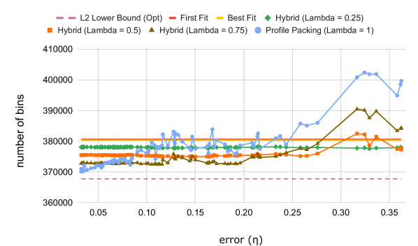
(a) Weibull distribution.

(b) GI benchmark from BPPLIB.

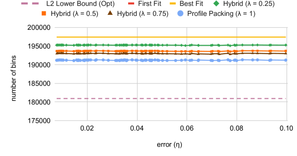
(c) Shwerin benchmark from BPPLIB.

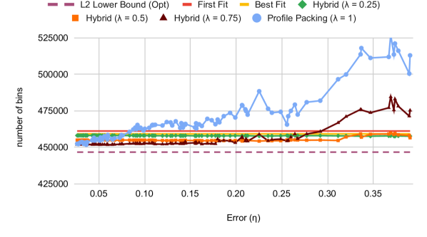
(d) Randomly_Generated benchmark from BPPLIB.

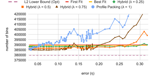
(e) Schoenfield_Hard28 benchmark from BPPLIB.

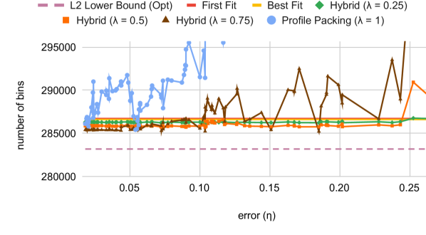
(f) Wäscher benchmark from BPPLIB.

Figure 1: Number of opened bins for sequences from a fixed distribution. For the purpose of visualization, some of the plots are truncated, e.g., the plot of ProfilePacking in (c) and (d).

Evolving distributions

We report experiments on the performance of Adaptive($w$). Recall that $w$ is the sliding window that determines how often the prediction is updated. This is a parameter that must be chosen judiciously: if $w$ is too small, we do not obtain sufficient information on the frequencies, whereas if $w$ is too big, the predictions become “stale”.

Figure 2 depicts the number of bins opened by Adaptive($w$) as a function of $w$ for different benchmarks. Here we report the average cost of the algorithms over 20 randomly generated sequences. We observe that for the benchmarks “Weibull" and “GI" benchmarks, there is a relatively wide range for $w$ that leads to marked performance improvement, in comparison to FirstFit and BestFit, namely $w\in[2100,25000]$. For the benchmarks “Randomly_Generated" and “Schoenfield_Hard28", we observe that Adaptive($w$) exhibits similar performance as the value of $w$ changes, that is, the number of opened bins is minimized when $w$ takes values in the range [2000,4000]; this holds also for “Schwerin" (Figure 2(c)) although the difference is marginal in this case. We also observe that for “Randomly_Generated" and “Schoenfield_Hard28", the performance curve of Adaptive($w$) is similar to that on the GI benchmark of the main paper.

When Adaptive($w$) opens a new profile group, the predicted frequencies are updated based on the $w$ most recently packed items. These $w$ items follow a distribution that may have changed since the time a new profile group was opened. As such, the performance of Adaptive($w$) depends on how diverse are the distributions that form the benchmark. In particular, for “Schwerin", the distribution does not evolve drastically, which explains why Adaptive($w$) performs consistently better than FirstFit and BestFit. This is not in case for the “Wäscher" benchmark, and here Adaptive($w$) does not offer any advantage over FirstFit and BestFit. Note, however, that these two baseline algorithms are remarkably close to the $L_{2}$ lower bound, which means that they output near-optimal packings for this benchmark, and which in turn leaves very little room for any potential improvement. These experiments demonstrate that even though Adaptive($w$) yields improvements in many situations, there are settings in which more sophisticated approaches will be required, as we explain in the Conclusions section of the main paper.

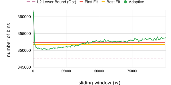
(a) Weibull distribution.

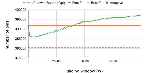
(b) GI benchmark from BPPLIB.

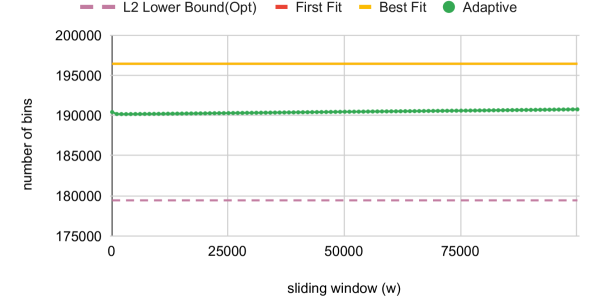
(c) Shwerin benchmark from BPPLIB.

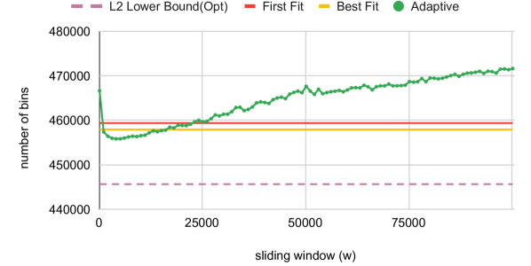
(d) Randomly_Generated benchmark from BPPLIB.

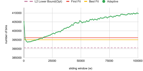
(e) Hard28 benchmark from BPPLIB.

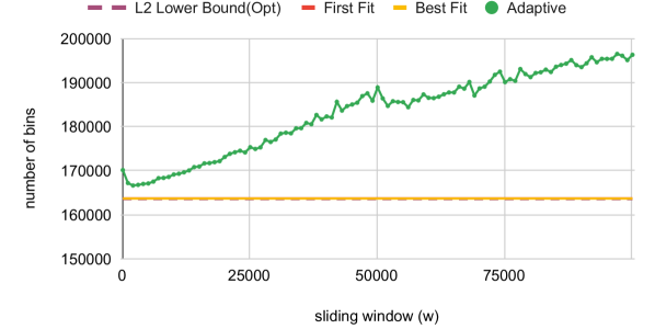
(f) Wäscher benchmark from BPPLIB.

Figure 2: Number of opened bins for sequences from an evolving distribution.

6.6 Experiments on the profile size

In previous experiments, we assumed that the profile size is $m=5000$. In this section we report experiments on other values of $m$. More precisely, we evaluated the performance on two sequences of length $n=10^{6}$ in which the item sizes are generated using Weibull distribution (with $sh=3$) and the GI-benchmark, respectively, as in Section 6.2. of the main paper. As before, we choose $k=100$. Predictions are generated based on a prefix of length $b=1000$ of the input; this corresponds to error values of $\eta=0.1922$ and $\eta=0.2045$ for the Weibull and GI-instances, respectively. We run Hybrid($\lambda$) ($\lambda\in\{0.25,0.5,0.75,1\}$) for $100$ different values of $m$, equidistant in $[100,100100]$.

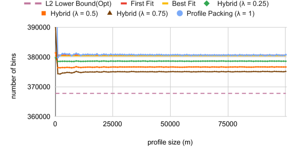
(a) Weibull benchmark.

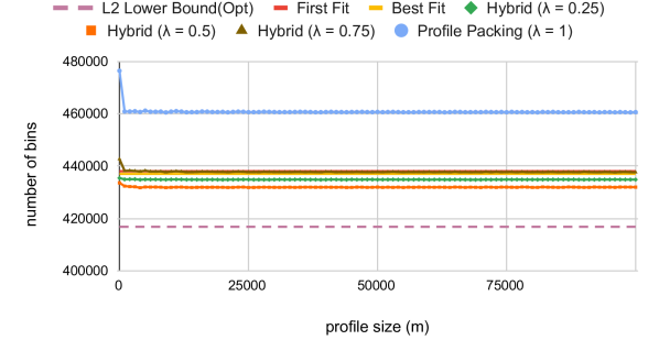
(b) GI benchmark from BPPLIB.

Figure 3: Number of opened bins as function of the profile size.

Figure 3 depicts the number of bins opened by the algorithms. The experiments show that the parameter $m$ has little impact on the performance of Hybrid($\lambda$), that is, as long as $m$ is sufficiently large (e.g., when $m\geq 1000$), the performance of Hybrid($\lambda$) is consistent and independent of the choice of $m$.

6.7 Further experiments on fixed distribution

In the experiments on Hybrid($\lambda$) for a fixed distribution that we presented in the main paper, we showed the performance of the algorithm on a typical sequence. More precisely, as explained in Section 6.5, we considered a single sequence, as opposed to averaging the cost of the algorithm over multiple input sequences, because each input sequence is associated with its own prediction error, for any given size of the prefix (and averaging over both the cost and the error may produce misleading results). We argued that this should not be an issue, because the input sequence is of considerable size ($n=10^{6}$), and the distribution is fixed.

In this section we present further experimental results based on averaging over both the cost and the error which give further justification for this choice. Our setting here is as follows: Given a fixed distribution (either Weibull with $sh=3$, or a file from the GI Benchmark), we generate 20 random sequences. For each sequence, we compute FirstFit, BestFit, and the $L2$ lower bound. The average costs of these algorithms, over the 20 sequences, serve as the benchmark costs for comparison.

For Hybrid($\lambda$), and every $\lambda\in[0.25,0.5,0.75,1]$, we generate predictions for $100$ values of the prefix size $b$ (where $b$ is of the form $b=100\cdot 1.05^{i}$, with $i\in[25,125]$, as in the main paper). Consider a sequence $\sigma$. For each of the above predictions for $\sigma$, we compute the prediction error as well as the cost of Hybrid($\lambda$) on $\sigma$ with the corresponding prediction and store a pair of the form (error, cost), where error is the error with a two-digit decimal precision, and the cost is the cost of the algorithm. For example, if error = 0.2341 and cost = 143000, we store the pair (0.23, 143000). This means that for a fixed sequence, we store up to 100 such pairs (assuming $\eta<1$). Last, we evaluate the average of pairs with the same rounded error over the 20 sequences. For example, if for $\sigma_{1}$ we have obtained the pair (0.23,100000), for $\sigma_{2}$ the pair (0.23, 150000), and for $\sigma_{3}$ the pair (0.23, 350000), then we take the average as the pair (0.23, 200000).

Figure 4 depicts the plots obtained by this method, for both the Weibull and the GI benchmarks. We observe that Hybrid($\lambda$) exhibits similar performance tradeoffs as the plots for a single sequence, namely Figure 1 in the main paper.

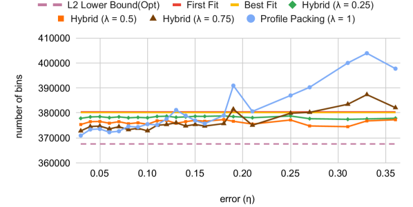
(a) Weibull benchmark.

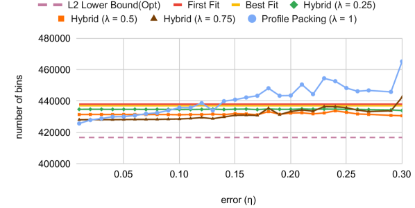
(b) GI Benchmark from BPPLIB.

Figure 4: Average number of bins vs average error over 20 sequences.

7 Conclusion

We gave the first results for online bin packing in a setting in which the algorithm has access to learnable predictions. We believe that our approach can be applicable to generalizations of the problem such as online vector bin packing [ACKS13]. Here, it will be crucial to devise time-efficient profile packing algorithms, since the profile size increases exponentially in the vector dimension.

Previous work on the experimental evaluation of online bin packing algorithms has focused on fixed input distributions. In our work we supplemented the analysis with a model for evolving input distributions, as well as a heuristic based on a sliding window. This should be considered only as a first step towards this direction. Future work needs to address more sophisticated input models and algorithms, drawn from the rich literature on evolving data streams; see e.g., the survey [KMG⁺17].

Appendix

A Details on the algorithms

A.1 ProfilePacking

Algorithm 1 describes ProfilePacking in pseudocode. Lines 1 to  9 are the initialization phase of the algorithm, in which the algorithm forms the profile set, computes an optimal packing of the profile set, and opens the first profile group. The optimal packing (Line 5) can be replaced by FirstFitDecreasing in order to reduce the time complexity, as we did in the experiments. The initial phase is followed by serving the sequence of requests in Lines 10 to 32. The algorithm maintains two multisets of bins in its packing. The multiset $\mathit{Empty}$, which describes the bins that are virtually opened but do not contain any item yet, and $\mathit{NonEmpty}$, which describes bins that contribute to the actual cost. When placing an item into either a bin of $\mathit{NonEmpty}$ (Lines 17) or $\mathit{Empty}$ (Lines 26), any bin with a placeholder of appropriate size can be selected. In our experiments, we break ties for bins in $\mathit{Empty}$ in favor of bins that contain a larger number of placeholders. This improves the typical performance of the algorithm.

A.2 Hybrid($\lambda$)

Algorithm 2 describes Hybrid($\lambda$) in pseudocode. This algorithm combines ProfilePacking and a given robust algorithm $A$. The initialization phase of Hybrid($\lambda$) is similar to that of ProfilePacking (Lines 1- 9 of Algorithm 1). As with ProfilePacking, for any $x\in[1,k]$, the algorithm maintains $N_{x}$ and $E_{x}$ as the set of $\mathit{NonEmpty}$ and $\mathit{Empty}$ bins with a placeholder of size $x$, respectively. The $i$-th item $\sigma[i]\in[1,k]$ is placed in a placeholder in $N_{x}$ and declared as PP-item if such a placeholder is available (Lines 9-12 of Algorithm 2). Otherwise, the item is declared as either PP-item (Lines 16-28) or A-item (Lines 30-31), depending on the frequency of PP-items of size $x$, and packed accordingly.

A.3 $H$-Aware

Algorithm 3 describes $H$-Aware in pseudocode. The algorithm receives as input an upper bound $H$ on the prediction error (i.e., we assume that $\eta\leq H$) and chooses between ProfilePacking (when $H$ is small) and a given robust algorithm $A$ (when $H$ is large). Note that the algorithm also receives a small value $\epsilon$ that is used to set the profile size parameter $m$ (we require that $m\geq 5k\tau_{k}/\epsilon$). For practical purposes, however, any large value of $m$ suffices. The running time of $H$-Aware is $O(kmn+A(k,n))$, where $A(k,n)$ denotes the running time of $A$. As in Hybrid($\lambda$), if $A$ is FirstFit, we have $A(k,n)=O(kn)$, and the time complexity of $H$-Aware becomes $O(kmn)$.

A.4 Adaptive($w$)

Algorithm 4 describes Adaptive($w$) in pseudocode. The algorithm packs the first $w$ items using the FirstFit strategy (Lines 9-10). From that point onwards, the algorithm maintains the number $c_{x}$ of items of size $x\in[1,k]$ among the last $w$ items (Lines 12-15). As in ProfilePacking, Adaptive($w$) maintains $N_{x}$ and $E_{x}$ as the set of bins in $\mathit{NonEmpty}$ and $\mathit{Empty}$ with an available placeholder for $x$. The algorithm places each item $\sigma[i]$ of size $x$ in a bin of $N_{x}$, if $N_{x}$ is not empty (Lines 17-19), and in a bin of $E_{x}$ (Lines 33-37), otherwise. If $E_{x}$ is empty, it opens a new profile group (Lines 22-31). If there is no placeholder available in $\mathit{NonEmpty}$ and $\mathit{Empty}$, the algorithm opens a new profile (Lines 34-28). In doing so, the algorithm generates item frequencies $\bm{f^{\prime}}$, as observed among the last $w$ items, to form a new profile set and an optimal packing of it.

$\triangleright$ packing items using ProfilePacking with parameter (profile size) $m$ into bins of capacity $k$. Input: $\sigma$: the input sequence with items in $[1,k]$ $\hskip 28.45274pt{\bm{f}^{\prime}}$: predicted item frequencies ($\forall x\in[1,k],{f^{\prime}_{x}}\in[0,1]$) Output: a packing of $\sigma$ (a set of bins that contain all items in $\sigma$)  
      $\triangleright$ form the profile set.

Algorithm 1 ProfilePacking

1:$P_{\bm{f}^{\prime}}\leftarrow\phi$  

2:for $x\in\{1,\ldots k\}$

3:    $P_{\bm{f}^{\prime}}\leftarrow P_{\bm{f}^{\prime}}\cup\{\lceil f^{\prime}_{x}m\rceil\text{ items of size }x\}$  

4: $\triangleright$ compute an optimal packing of the profile set in which each bin is partitioned to placeholders.

5:$\textsc{Opt}_{\bm{f^{\prime}}}(P)=$ optimal packing of $P_{\bm{f^{\prime}}}$.

6: $p_{f^{\prime}}\leftarrow|\textsc{Opt}_{\bm{f^{\prime}}}(P)|$

7:$\mathit{Group}$ $\ \leftarrow$ $p_{f^{\prime}}$ empty bins in accordance with $\textsc{Opt}_{\bm{f^{\prime}}}(P)$. $\triangleright$ open the first profile group

8:$\mathit{Empty}$ $\ \leftarrow$ $\mathit{Group}$ $\triangleright$ bins that are opened but empty

9:$\mathit{NonEmpty}$ $\ \leftarrow\phi$ $\triangleright$ bins that contribute to the cost

10:for $i\in(1,\ldots,n)$ do $\triangleright$ packing the sequence in an online manner

11:    $x\leftarrow\sigma[i]$

12:   if $\textsc{Opt}_{\bm{f^{\prime}}}(P)$ has no placeholder of size $x$ then

13:      use FirstFit to pack $\sigma[i]$ $\triangleright$  $x$ is a special item

14:   else

15:      $N_{x}\leftarrow$ bins in $\mathit{NonEmpty}$ with placeholder for $x$

16:      if $N_{x}\neq\phi$ then $\triangleright$ place $\sigma[i]$ in a non-empty bin

17:         $B\leftarrow$ any bin of $N_{x}$

18:         place $\sigma[i]$ in a placeholder of size $x$ in $B$

19:      else

20:         $E_{x}\leftarrow$ bins in $\mathit{Empty}$ with placeholder for $x$

21:         if $E_{x}=\phi$ then             $\triangleright$ open a new profile group

22:            $\mathit{Group}$ $\ \leftarrow$ $p_{f^{\prime}}$ new bins as in $\textsc{Opt}_{\bm{f^{\prime}}}(P)$

23:            $\mathit{Empty}$ $\ \leftarrow$ $\mathit{Empty}$ $\ \cup$ $\mathit{Group}$  

24:         end if            

25: $\triangleright$ place $\sigma[i]$ in a (virtually) opened empty bin

26:         $B\leftarrow$ any bin of $E_{x}$

27:         place $\sigma[i]$ in a placeholder of size $x$ in $B$

28:         $\mathit{Empty}$ $\ \leftarrow$ $\mathit{Empty}$ $\setminus\ \{B\}$

29:         $\mathit{NonEmpty}$ $\ \leftarrow$ $\mathit{NonEmpty}$ $\ \cup\ \{B\}$

30:      end if

31:   end if

32:end for  

33:return $\mathit{NonEmpty}$ $\triangleright$ return the set of non-empty bins

$\triangleright$ packing items using Hybrid($\lambda$) that combines ProfilePacking with parameter $m$ and robust algorithm $A$ to pack an input sequence into bins of capacity $k$. Input: $\sigma$: the input sequence with items in $[1,k]$ ${\bm{f}^{\prime}}$: predicted item frequencies ($\forall x\in[1,k],{f^{\prime}_{x}}\in[0,1]$) Output: a packing of $\sigma$ (a set of bins that contain all items in $\sigma$)

Algorithm 2 Hybrid($\lambda$)

1:Initialize ProfilePacking (Lines 1- 9 of Algorithm 1)

2:for $x\in\{1,\ldots k\}$ do

3:   ${\tt count}(x)$, ${\tt ppcount}(x)$ $\leftarrow 0$  

4:end for

5:for $i\in(1,\ldots,n)$ do $\triangleright$ packing the sequence in an online manner

6:    $x\leftarrow\sigma[i]$

7:   ${\tt count}(x)$ $\ \leftarrow\$ ${\tt count}(x)$ $+1$

8:   $N_{x}\leftarrow$ bins in $\mathit{NonEmpty}$ with a placeholder for $x$

9:   if $N_{x}\neq\phi$ then

10:      ${\tt ppcount}(x)$ $\ \leftarrow\$ ${\tt ppcount}(x)$ $+1$ $\triangleright$  $\sigma[i]$ is treated as a pp-item

11:      $B\leftarrow$ any bin of $N_{x}$

12:      place $\sigma[i]$ in a placeholder of size $x$ in $B$

13:   else

14:       $\triangleright$ decide between ProfilePacking and $A$

15:      if ${\tt ppcount}(x)$ $\leq\lambda$ ${\tt ppcount}(x)$ then $\triangleright$  $\sigma[i]$ is treated as a pp-item

16:         ${\tt ppcount}(x)$ $\ \leftarrow\$ ${\tt ppcount}(x)$ $+1$

17:         if $\textsc{Opt}_{\bm{f^{\prime}}}(P)$ has no placeholder of size $x$ then

18:            use FirstFit to pack $\sigma[i]$ $\triangleright$  $x$ is a special item

19:         else

20:            $E_{x}\leftarrow$ bins in $\mathit{Empty}$ with placeholder for $x$

21:            if $E_{x}=\phi$ then                $\triangleright$ open a new profile group

22:               $\mathit{Group}$ $\ \leftarrow$ $p_{f^{\prime}}$ new bins as in $\textsc{Opt}_{\bm{f^{\prime}}}(P)$          

23:               $\mathit{Empty}$ $\ \leftarrow$ $\mathit{Empty}$ $\ \cup$ $\mathit{Group}$  

24:            end if

25:            $B\leftarrow$ any bin of $E_{x}$ $\triangleright$ place $\sigma[i]$ in a (virtually) opened empty bin

26:            place $\sigma[i]$ in placeholder of size $x$ in $B$

27:            $\mathit{Empty}$ $\ \leftarrow$ $\mathit{Empty}$ $\setminus\{B\}$

28:            $\mathit{NonEmpty}$ $\ \leftarrow$ $\mathit{NonEmpty}$ $\ \cup\ \{B\}$

29:         end if

30:      else

31:         use $A$ to pack $x$      $\triangleright$  $\sigma[i]$ is treated as an A-item

32:      end if

33:   end if

34:end for 

35:return $\mathit{NonEmpty}$ $\triangleright$ return the set of non-empty bins

$\triangleright$ packing items using $H$-Aware that chooses between ProfilePacking with parameter $m$ and robust algorithm $A$ with competitive ratio $c_{A}$ to pack an input sequence into bins of capacity $k$. Input: $\sigma$: the input sequence with items in $[1,k]$ ${\bm{f}^{\prime}}$: predicted item frequencies ($\forall x\in[1,k],{f^{\prime}_{x}}\in[0,1]$) ${H}$: an upper bound on error ($\eta\leq H$) ${\epsilon}$: a small positive value ($\epsilon<0.2$) Output: a packing of $\sigma$ (a set of bins that contain all items in $\sigma$)

Algorithm 3 $H$-Aware

1:$Packing=\phi$ $\triangleright$ the resulting packing

2:if $H<(c_{A}-1-\epsilon)/(k(2+5\epsilon))$ then

3: $\triangleright$ Error cannot be large; use ProfilePacking

4:   $Packing=\textsc{ProfilePacking}(\sigma,f^{\prime})$

5:else

6: $\triangleright$ Error can be large; ignore predictions and use $A$

7:   $Packing=A(\sigma)$

8:end if

9:return $Packing$ $\triangleright$ return the set of non-empty bins

$\triangleright$ packing items using Adaptive($w$) with sliding window $w$ and profile size $m$. Input:
$\sigma$: the input sequence with items in $[1,k]$ Output:
a packing of $\sigma$ (a set of bins that contain all items in $\sigma$)

Algorithm 4 $\textsc{Adaptive}($w$)$

1:$\mathit{Empty}$ $\ \leftarrow\phi$ $\triangleright$ bins that are opened but empty

2:$\mathit{NonEmpty}$ $\ \leftarrow\phi$ $\triangleright$ bins that contribute to the cost  

3:for $x\in\{1,\ldots,k\}$

4:    $c_{x}\leftarrow 0$ $\triangleright$ no. items of size $x$ among the last $w$ items

5: $\triangleright$ packing the sequence in an online manner

6:for $i\in(1,\ldots,n)$ do

7:    $x\leftarrow\sigma[i]$

8:   $c_{x}\leftarrow c_{x}+1$

9:   if $i\leq w$ then                            

10:      use FirstFit to pack $x$ $\triangleright$ initial phase

11:   else

12:       $\triangleright$ updating frequencies in the last $w$ requests

13:      $y\leftarrow\sigma[i-w]$

14:      $c_{y}\leftarrow c_{y}-1$

15:   end if

16:   $N_{x}\leftarrow$ bins in $\mathit{NonEmpty}$ with a placeholder for $x$

17:   if $N_{x}\neq\phi$ then $\triangleright$ place $\sigma[i]$ in a non-empty bin

18:      $B\leftarrow$ any bin of $N_{x}$

19:      place $\sigma[i]$ in a placeholder of size $x$ in $B$

20:   else

21:      $E_{x}\leftarrow$ bins in $\mathit{Empty}$ with placeholder for $x$

22:      if $E_{x}=\phi$ then          $\triangleright$ open a new profile group

23:         $P_{\bm{f}^{\prime}}\leftarrow\phi$

24:         for $x\in\{1,\ldots k\}$ do

25:            $f^{\prime}_{x}\leftarrow c_{x}/w$

26:            $P_{\bm{f}^{\prime}}\leftarrow P_{\bm{f}^{\prime}}\cup\{\lceil f^{\prime}_{x}m\rceil\text{ items of size }x\}$  

27:         end for

28:         $\textsc{Opt}_{\bm{f^{\prime}}}(P)=$ optimal packing of $P_{\bm{f^{\prime}}}$.

29:          $p_{f^{\prime}}\leftarrow|\textsc{Opt}_{\bm{f^{\prime}}}(P)|$

30:         $\mathit{Group}$ $\ \leftarrow$ $p_{f^{\prime}}$ bins in accordance to $\textsc{Opt}_{\bm{f^{\prime}}}(P)$.

31:         $\mathit{Empty}$ $\ \leftarrow$ $\mathit{Empty}$ $\ \cup$ $\mathit{Group}$  

32:      end if 

33:       $\triangleright$ place $\sigma[i]$ in a (virtually) opened empty bin

34:      $B\leftarrow$ any bin of $E_{x}$

35:      place $\sigma[i]$ in a placeholder of size $x$ in $B$

36:      $\mathit{Empty}$ $\ \leftarrow$ $\mathit{Empty}$ $\setminus\ \{B\}$

37:      $\mathit{NonEmpty}$ $\ \leftarrow$ $\mathit{NonEmpty}$ $\ \cup\ \{B\}$

38:   end if

39:end forreturn $\mathit{NonEmpty}$ $\triangleright$ return the set of non-empty bins

References

- [ACE+20] Antonios Antoniadis, Christian Coester, Marek Eliás, Adam Polak, and Bertrand Simon. Online metric algorithms with untrusted predictions. In Proceedings of the 37th International Conference on Machine Learning (ICML), pages 345–355, 2020.
- [ACKS13] Yossi Azar, Ilan Reuven Cohen, Seny Kamara, and Bruce Shepherd. Tight bounds for online vector bin packing. In Proceedings of the 45th Annual ACM Symposium on Theory of Computing (STOC), pages 961–970, 2013.
- [ADJ+20] Spyros Angelopoulos, Christoph Dürr, Shendan Jin, Shahin Kamali, and Marc P. Renault. Online computation with untrusted advice. In Proceedings of the 11th Innovations in Theoretical Computer Science Conference (ITCS), pages 52:1–52:15, 2020.
- [ADK+18] Spyros Angelopoulos, Christoph Dürr, Shahin Kamali, Marc P. Renault, and Adi Rosén. Online bin packing with advice of small size. Theory of Computing Systems, 62(8):2006–2034, 2018.
- [AGKK20] Antonios Antoniadis, Themis Gouleakis, Pieter Kleer, and Pavel Kolev. Secretary and online matching problems with machine learned advice. In Proceedings of the 33rd Conference on Neural Information Processing Systems (NeurIPS), 2020.
- [AGP20] Keerti Anand, Rong Ge, and Debmalya Panigrahi. Customizing ML predictions for online algorithms. In International Conference on Machine Learning (ICML), pages 303–313. PMLR, 2020.
- [Ban20] Soumya Banerjee. Improving online rent-or-buy algorithms with sequential decision making and ML predictions. In Proceedings of the 33rd Conference on Neural Information Processing Systems (NeurIPS), 2020.
- [BB12] Anton Beloglazov and Rajkumar Buyya. Optimal online deterministic algorithms and adaptive heuristics for energy and performance efficient dynamic consolidation of virtual machines in cloud data centers. Concurr. Comput. Pract. Exp., 24(13):1397–1420, 2012.
- [BBD+18] János Balogh, József Békési, György Dósa, Leah Epstein, and Asaf Levin. A new and improved algorithm for online bin packing. In Proceedings of the 26th European Symposium on Algorithms (ESA), volume 112, pages 5:1–5:14, 2018.
- [BBG12] János Balogh, József Békési, and Gábor Galambos. New lower bounds for certain classes of bin packing algorithms. Theoretical Computer Science, 440:1–13, 2012.
- [BBV11] Doina Bein, Wolfgang Bein, and Swathi Venigella. Cloud storage and online bin packing. In Proceedings of the 5th International Symposium on Intelligent Distributed Computing (IDC), pages 63–68. Springer, 2011.
- [BKLL16] Joan Boyar, Shahin Kamali, Kim S. Larsen, and Alejandro López-Ortiz. Online bin packing with advice. Algorithmica, 74(1):507–527, 2016.
- [Can20] Clément L. Canonne. A short note on learning discrete distributions, 2020. arXiv math.ST:2002.11457.
- [CCO12] Ignacio Castiñeiras, Milan De Cauwer, and Barry O’Sullivan. Weibull-based benchmarks for bin packing. In Proceedings of the 18th International Conference on Principles and Practice of Constraint Programming (CP), volume 7514, pages 207–222, 2012.
- [CGJ96] E. G. Coffman, M. R. Garey, and D. S. Johnson. Approximation algorithms for bin packing: A survey. In Approximation Algorithms for NP-Hard Problems, page 46–93. Springer, 1996.
- [CJK+06] Janos Csirik, David S Johnson, Claire Kenyon, James B Orlin, Peter W Shor, and Richard R Weber. On the sum-of-squares algorithm for bin packing. Journal of the ACM (JACM), 53(1):1–65, 2006.
- [CKPT17] Henrik I. Christensen, Arindam Khan, Sebastian Pokutta, and Prasad Tetali. Approximation and online algorithms for multidimensional bin packing: A survey. Comput. Sci. Rev., 24:63–79, 2017.
- [DIM] M. Delorme, M. Iori, and S. Martello. BPPLIB–a bin packing problem library. http://or.dei.unibo.it/library/bpplib, Accessed: 2021-05-2.
- [DIM14] Maxence Delorme, Manuel Iori, and Silvano Martello. Bin packing and cutting stock problems: mathematical models and exact algorithms. In Decision models for smarter cities, 2014.
- [FK07] Alex S. Fukunaga and Richard E. Korf. Bin completion algorithms for multicontainer packing, knapsack, and covering problems. Journal of Artificial Intelligence Research (JAIR), 28:393–429, 2007.
- [GBEB17] Heitor Murilo Gomes, Jean Paul Barddal, Fabrício Enembreck, and Albert Bifet. A survey on ensemble learning for data stream classification. ACM Computing Surveys (CSUR), 50(2):1–36, 2017.
- [Gen98] Ian P. Gent. Heuristic solution of open bin packing problems. Journal of Heuristics, 3(4):299–304, 1998.
- [GI16] Timo Gschwind and Stefan Irnich. Dual inequalities for stabilized column generation revisited. INFORMS Journal on Computing, 28(1):175–194, 2016.
- [GLO10] András György, Gábor Lugosi, and György Ottucsák. On-line sequential bin packing. Journal of Machine Learning Research, 11:89–109, 2010.
- [GP19] Sreenivas Gollapudi and Debmalya Panigrahi. Online algorithms for rent-or-buy with expert advice. In Proceedings of the 36th International Conference on Machine Learning (ICML), pages 2319–2327, 2019.
- [GR20] Varun Gupta and Ana Radovanovic. Interior-point-based online stochastic bin packing. Operations Research, 68(5):1474–1492, 2020.
- [JDU+74] David S. Johnson, A. Demers, J. D. Ullman, Michael R. Garey, and Ronald L. Graham. Worst-case performance bounds for simple one-dimensional packing algorithms. SIAM Journal on Computing (SICOMP), 3:256–278, 1974.
- [KLO15] Shahin Kamali and Alejandro López-Ortiz. All-around near-optimal solutions for the online bin packing problem. In International Symposium on Algorithms and Computation (ISAAC), pages 727–739, 2015.
- [KMG+17] Bartosz Krawczyk, Leandro L Minku, João Gama, Jerzy Stefanowski, and Michał Woźniak. Ensemble learning for data stream analysis: A survey. Information Fusion, 37:132–156, 2017.
- [Kor02] Richard E. Korf. A new algorithm for optimal bin packing. In Proceedings of the 18th AAAI Conference on Artificial Intelligence, pages 731–736, 2002.
- [Kor03] Richard E. Korf. An improved algorithm for optimal bin packing. In Proceedings of the 18th International Joint Conference on Artificial Intelligence (IJCAI), pages 1252–1258, 2003.
- [LLMV20] Silvio Lattanzi, Thomas Lavastida, Benjamin Moseley, and Sergei Vassilvitskii. Online scheduling via learned weights. In Proceedings of the 14th ACM-SIAM Symposium on Discrete Algorithms (SODA), pages 1859–1877, 2020.
- [LMRX20] Thomas Lavastida, Benjamin Moseley, R. Ravi, and Chenyang Xu. Learnable and instance-robust predictions for online matching, flows and load balancing. CoRR, abs/2011.11743, 2020.
- [LV18] Thodoris Lykouris and Sergei Vassilvitskii. Competitive caching with machine learned advice. In Proceedings of the 35th International Conference on Machine Learning (ICML), pages 3302–3311, 2018.
- [Mik16] Jesper W. Mikkelsen. Randomization can be as helpful as a glimpse of the future in online computation. In Proceedings of the 43rd International Colloquium on Automata, Languages, and Programming (ICALP), volume 55, pages 39:1–39:14, 2016.
- [MT90] Silvano Martello and Paolo Toth. Lower bounds and reduction procedures for the bin packing problem. Discrete Applied Mathematics, 28(1):59–70, 1990.
- [MV20] M. Mitzenmacher and S. Vassilvitskii. Algorithms with predictions. In Tim Roughgarden, editor, Beyond the Worst-Case Analysis of Algorithms, pages 646–662. Cambridge University Press, 2020.
-
[Ove10]
Intel Executive Overview.
Implementing and expanding a virtualized environment, 2010.
https://www.intel.com/content/dam/www/public/us/en/documents/white-papers/intel-it-virtualization-best-practices-paper.pdf,
accessed: 2021-05-25. - [PSK18] Manish Purohit, Zoya Svitkina, and Ravi Kumar. Improving online algorithms via ML predictions. In Proceedings of the 31st Conference on Neural Information Processing Systems (NeurIPS), volume 31, pages 9661–9670, 2018.
- [Roh20] Dhruv Rohatgi. Near-optimal bounds for online caching with machine learned advice. In Proceedings of the 14th ACM-SIAM Symposium on Discrete Algorithms (SODA), pages 1834–1845, 2020.
- [Sch02] Jon E. Schoenfield. Fast, exact solution of open bin packing problems without linear programming. Draft, US Army Space and Missile Defense Command, 2002.
- [SK13] Ethan L. Schreiber and Richard E. Korf. Improved bin completion for optimal bin packing and number partitioning. In Proceedings of the 23rd International Joint Conference on Artificial Intelligence (IJCAI), pages 651–658, 2013.
- [SW97] Petra Schwerin and Gerhard Wäscher. The bin-packing problem: A problem generator and some numerical experiments with ffd packing and mtp. International Transactions in Operational Research, 5(4):377–389, 1997.
- [SXCL13] Weijia Song, Zhen Xiao, Qi Chen, and Haipeng Luo. Adaptive resource provisioning for the cloud using online bin packing. IEEE Transactions on Computers, 63(11):2647–2660, 2013.
- [VMw] VMware. Server consolidation. https://www.vmware.com/ca/solutions/consolidation.html, accessed: 2021-05-25.
- [WG96] Gerhard Wäscher and Thomas Gau. Heuristics for the integer one-dimensional cutting stock problem: A computational study. Operations-Research-Spektrum, 18(3):131–144, 1996.
- [WMZ11] Meng Wang, Xiaoqiao Meng, and Li Zhang. Consolidating virtual machines with dynamic bandwidth demand in data centers. In Proceedings of the 30th IEEE Conference on Computer Communications (INFOCOM), pages 71–75, 2011.
- [WZ20] Alexander Wei and Fred Zhang. Optimal robustness-consistency trade-offs for learning-augmented online algorithms. In Proceedings of the 34th Annual Conference on Neural Information Processing Systems (NeurIPS), 2020.