Phantom Bethe roots in the integrable open spin-$\frac{1}{2}$ XXZ chain

Abstract

We investigate special solutions to the Bethe Ansatz equations (BAE) for open integrable XXZ Heisenberg spin chains containing phantom (infinite) Bethe roots. The phantom Bethe roots do not contribute to the energy of the Bethe state, so the energy is determined exclusively by the remaining regular excitations. We derive the phantom Bethe roots criterion and focus on BAE solutions for mixtures of phantom roots and regular (finite) Bethe roots. We prove that in the presence of phantom Bethe roots, all eigenstates are split between two invariant subspaces, spanned by chiral shock states. Bethe eigenstates are described by two complementary sets of Bethe Ansatz equations for regular roots, one for each invariant subspace. The respective “semi-phantom” Bethe vectors are states of chiral nature, with chirality properties getting less pronounced when more regular Bethe roots are added. For the easy plane case “semi-phantom” Bethe states carry nonzero magnetic current, and are characterized by quasi-periodic modulation of the magnetization profile, the most prominent example being the spin helix states (SHS). We illustrate our results investigating “semi-phantom” Bethe states generated by one regular Bethe root (the other Bethe roots being phantom), with simple structure of the invariant subspace, in all details. We obtain the explicit expressions for Bethe vectors, and calculate the simplest correlation functions, including the spin-current for all the states in the single particle multiplet.

I Introduction

Contemporary experimental techniques allow to realize almost perfect one-dimensional XXZ spin chains with adjustable anisotropy 2020NatureSpinHelix . The spin-$\frac{1}{2}$ XXZ chain, being an integrable interacting many-body system, is one of the best studied paradigmatic models in quantum statistical mechanics GaudinBook . Ongoing advances make the XXZ model a source of inspiration and fascinating new discoveries, such as finding a set of quasilocal conservation laws 2013ProsenQuasilocal , calculating finite temperature correlation functions GoehmannKluemperSeel ; BoosGoehmann , and giving a major contribution to the theory of finite-temperature quantum transport 2020BertiniReview .

In our letter PhantomShort we have shown that SHS correspond to a novel type of Bethe roots, phantom “singular” Bethe roots in the Bethe Ansatz equations. These exotic Bethe roots describe excitations, which do not contribute to the energy of the system. We show that the presence of such excitations leads to highly atypical chiral XXZ eigenstates carrying nonzero spin currents and exhibiting periodic modulations of the magnetization density profile. We have established a criterion for the presence of phantom Bethe roots, for both periodic and open boundaries, and investigated phantom Bethe states formed exclusively from phantom Bethe excitations.

In the present manuscript we treat the most challenging case of an open XXZ Hamiltonian with non-diagonal boundary fields. The Bethe Ansatz equations for the spectrum have been formally constructed OffDiagonal ; Cao2013off ; Zhang2015 for the general integrable open chain. The separation of variables method has been applied to this model in Niccoli2012 ; Faldella2014 ; Kitanine2014 . And under a certain compatibility condition the so-called alternative modified Algebraic Bethe Ansatz approach OffDiagonal03 ; Belliard was successful. Despite these works little is known about the solutions to the eigenvalue equations and even less is known about the structure of the eigenstates. Here we demonstrate that in presence of any number of phantom Bethe roots the Hilbert space of the system is split into two blocks, invariant with respect to the action of the Hamiltonian. The condition for the splitting coincides with the condition needed for the applicability of the alternative modified Algebraic Bethe Ansatz OffDiagonal03 ; Belliard and a conventional Baxter’s $T$-$Q$ relation OffDiagonal .

We refer to our finding as the “splitting theorem” which gives us a tool to study the structure of phantom Bethe states, belonging to each invariant subspace, and to show that “semi-phantom” Bethe states retain the chiral character of “fully-phantom” spin-helix states, as long as the number of regular Bethe roots involved remains small in comparison to the system size. In special cases the explicit form of phantom Bethe states and various observables including spin magnetization current can be calculated analytically.

The plan of the paper is the following. After introducing the model we remind of the concept of phantom Bethe roots, and derive the phantom Bethe roots existence criterion. Next, we prove the theorem about the splitting of the Hilbert space into two invariant chiral subspaces, and describe the basis states spanning them. In the final part of the manuscript we use the gained knowledge to investigate the phantom Bethe states belonging to the invariant subspace with dimension $N+1$ where $N$ is the length of the XXZ spin chain. Details of the proofs are given in the Appendix.

II Phantom Bethe roots in the open XXZ chain

We consider the XXZ spin-$\frac{1}{2}$ chain with open boundaries. The Hamiltonian reads

$$H=\sum_{n=1}^{N-1}h_{n,n+1}+h_{1}+h_{N},$$ (1)

with

$$h_{n,n+1}=\sigma_{n}^{x}\sigma_{n+1}^{x}+\sigma_{n}^{y}\sigma_{n+1}^{y}+{\cosh}\eta\sigma_{n}^{z}\sigma_{n+1}^{z}-{\cosh}\eta\,I,$$ (2)

$$h_{1}=\frac{{\sinh}\eta}{{\sinh}(\alpha_{-}){\cosh}(\beta_{-})}({\cosh}(\theta_{-})\sigma_{1}^{x}+\mathrm{i}\,{\sinh}(\theta_{-})\sigma_{1}^{y}+{\cosh}(\alpha_{-}){\sinh}(\beta_{-})\sigma_{1}^{z}),$$ (3)

$$h_{N}=\frac{{\sinh}\eta}{{\sinh}(\alpha_{+}){\cosh}(\beta_{+})}({\cosh}(\theta_{+})\sigma_{N}^{x}+\mathrm{i}\,{\sinh}(\theta_{+})\sigma_{N}^{y}-{\cosh}(\alpha_{+}){\sinh}(\beta_{+})\sigma_{N}^{z}).$$ (4)

Here $\alpha_{\pm}$, $\beta_{\pm}$ and $\theta_{\pm}$ are boundary parameters. The system (1) is integrable OffDiagonal and its exact solutions are given by the off-diagonal Bethe Ansatz (ODBA) method OffDiagonal ; Cao2013off ; Zhang2015 and the separation of variables method Niccoli2012 ; Faldella2014 ; Kitanine2014 .

Under generic open boundary conditions, the exact solutions of the system are given by an unconventional $T$-$Q$ relation with inhomogeneous term OffDiagonal ; Cao2013off , resulting in a set of BAE with $N$ so-called Bethe roots $\{\mu_{1},\dots,\mu_{N}\}$

$$\frac{2G(-\mu_{j}\!-\!\frac{\eta}{2})Q(-\mu_{j}\!-\!\frac{\eta}{2})}{\sinh(2\mu_{j}\!+\!\eta)\sinh^{2N}(\mu_{j}\!+\!\frac{\eta}{2})}+\frac{2G(\mu_{j}\!-\!\frac{\eta}{2})Q(\mu_{j}\!-\!\frac{\eta}{2})}{\sinh(2\mu_{j}\!-\!\eta)\sinh^{2N}(\mu_{j}\!-\!\frac{\eta}{2})}=c\sinh(2\mu_{j}),\qquad j=1,\ldots,N,$$ (5)

$$Q(u)=\prod_{k=1}^{N}\sinh(u-\mu_{k}-\frac{\eta}{2})\sinh(u+\mu_{k}-\frac{\eta}{2}),$$

$$G(u)=\prod_{\sigma=\pm}\sinh(u-\alpha_{\sigma})\cosh(u-\beta_{\sigma})\,,$$

$$c=\cosh\left[(N+1)\eta+\alpha_{-}+\beta_{-}+\alpha_{+}+\beta_{+}\right]-\cosh(\theta_{-}-\theta_{+})\,.$$ (6)

All eigenvalues of the Hamiltonian (1) are classified by different sets of Bethe roots $\{\mu_{j}\}$ as

$$E=\sum_{j=1}^{N}\frac{4\sinh^{2}\eta}{\cosh(2\mu_{j})-\cosh\eta}+E_{0},$$ (7)

$$E_{0}=-{\sinh}\eta\left(\coth(\alpha_{-})+\tanh(\beta_{-})+\coth(\alpha_{+})+\tanh(\beta_{+})\right).$$ (8)

Note that unlike the periodic chain and the open chain with diagonal boundary fields which preserve the $U(1)$ symmetry, here each eigenstate and the corresponding eigenvalue are characterized by a set of Bethe roots $\{\mu_{j}\}$ with strictly $N$ members. Typically, it is taken for granted that all $\{\mu_{j}\}_{j=1}^{N}$ are bounded, so that every Bethe root gives a nonzero contribution to the energy (7). However, it was pointed out by us PhantomShort , that unbounded “phantom” solutions of BAE (5) do exist, which lead to “phantom” excitations not contributing to the energy. For completeness, below we give the definition and the derivation of the phantom Bethe roots existence criterion.

Definition. We shall call a Bethe root $\mu_{p}$ satisfying (5), a phantom Bethe root, if it does not give a contribution to the respective energy eigenvalue (7) i.e. if

$${\rm Re}[\mu_{p}]=\pm\infty.$$ (9)

We assume that, out of $N$ Bethe roots, $N-M$ roots are phantom,

$$\mu_{p}=\infty+\gamma_{p},\ \ \ p=1,2,\ldots N-M,$$ (10)

where $\gamma_{p}$ are some finite imaginary constants. The more precise formulation of (10) is $\mu_{p}=\mu_{\infty}+\gamma_{p}$ with $\mu_{\infty}\to\infty$. The remaining $M$ Bethe roots $\mu_{N-M+1},\mu_{N-M+2},\ldots,\mu_{N}$ are supposed to remain finite. In this situation, the BAE decouple for the phantom roots and the regular roots. Inserting (10) into (5), for $1\leq p\leq N-M$ we obtain

$$\mathsf{e}^{W}\prod_{k=1}^{N-M}2\mathsf{e}^{\gamma_{k}-\gamma_{p}}\sinh(\gamma_{p}-\gamma_{k}+\eta)+\mathsf{e}^{-W}\prod_{k=1}^{N-M}2\mathsf{e}^{\gamma_{k}-\gamma_{p}}\sinh(\gamma_{p}-\gamma_{k}-\eta)=2c,$$ (11)

$$W=(M+1)\eta+\alpha_{-}+\beta_{-}+\alpha_{+}+\beta_{+}.$$

Let us use the Ansatz

$$\gamma_{k}=\mathrm{i}\pi k/(N-M),$$ (12)

and denote $\omega=\mathsf{e}^{\mathrm{i}\pi/(N-M)}$, so that $\omega^{N-M}=-1$ and $\mathsf{e}^{\gamma_{k}}=\omega^{k}$. Then we can rewrite the first term on the LHS of (11) as

$$\prod_{k=1}^{N-M}\mathsf{e}^{\gamma_{k}-\gamma_{p}}(2\sinh(\gamma_{p}-\gamma_{k}+\eta))=\mathsf{e}^{(N-M)\eta}\prod_{n=1}^{N-M}\left(1-\omega^{2n-2}\mathsf{e}^{-2\eta}\right)$$

$$=\mathsf{e}^{(N-M)\eta}\left(1\!-\!\mathsf{e}^{-2\eta(N-M)}\right)\!=\!2\sinh((N\!-\!M)\eta),$$ (13)

where we used the identity

$$\prod_{n=1}^{N-M}\left(1-\omega^{2n-2}z\right)=1-z^{N-M}\,,$$ (14)

as both sides are polynomials of degree $N-M$ in $z$, share the same zeros and have identical $0$-th order coefficient. For $z=\mathsf{e}^{-2\eta}$ the RHS of (14) reduces to the term in brackets of line (13). Analogously, we obtain

$$\prod_{k=1}^{N-M}2\mathsf{e}^{\gamma_{k}-\gamma_{j}}\sinh(\gamma_{j}-\gamma_{k}-\eta)=-2\sinh((N-M)\eta).$$ (15)

The LHS of (11) can thus be rewritten as

$$4\sinh W\sinh((N-M)\eta)=2\cosh((N-M)\eta+W)-2\cosh((N-M)\eta-W)=2c.$$ (16)

Recalling the definition of $W$ in (11) and $c$ in (6) we note that $2c=2\cosh((N-M)\eta+W)-2\cosh(\theta_{-}-\theta_{+})$. In order to satisfy (16) we must require $\cosh(\theta_{-}-\theta_{+})=\cosh((N-M)\eta-W)$, i.e.

$$\pm(\theta_{+}-\theta_{-}) =(2M-N+1)\eta+\alpha_{-}+\beta_{-}+\alpha_{+}+\beta_{+}\ \mod 2\pi\mathrm{i}.$$ (17)

Therefore, under condition (17), $N-M$ out of $N$ Bethe roots in (5) can be chosen phantom. Integer $M$ naturally has the range $0\leq M<N$.

To obtain the BAE for the $M$ remaining finite roots $x_{j}=\mu_{N-M+j}$, we substitute (10) into (5) and take $j>N-M$. The LHS of (5) contains factoring divergent terms, so that the finite constant $2c$ on the RHS of (5) can be neglected. The leading order gives the final BAE OffDiagonal03 ; Rafael2003 ; Nepomechie2003

$$\left[\frac{{\sinh}(x_{j}+\frac{\eta}{2})}{{\sinh}(x_{j}-\frac{\eta}{2})}\right]^{2N}\prod_{\sigma=\pm}\frac{{\sinh}(x_{j}-\alpha_{\sigma}-\frac{\eta}{2})}{{\sinh}(x_{j}+\alpha_{\sigma}+\frac{\eta}{2})}\frac{{\cosh}(x_{j}-\beta_{\sigma}-\frac{\eta}{2})}{{\cosh}(x_{j}+\beta_{\sigma}+\frac{\eta}{2})}$$

$$=\prod_{k\neq j}^{M}\frac{{\sinh}(x_{j}-x_{k}+\eta)\,{\sinh}(x_{j}+x_{k}+\eta)}{{\sinh}(x_{j}-x_{k}-\eta)\,{\sinh}(x_{j}+x_{k}-\eta)},\quad j=1,\ldots,M.$$ (18)

while the respective energy has contributions from the $M$ finite Bethe roots only,

$$E=\sum_{j=1}^{M}\frac{4{\sinh}^{2}\eta}{{\cosh}(2x_{j})-{\cosh}\eta}+E_{0}.$$ (19)

The condition (17) has been derived in OffDiagonal03 ; Nepomechie2003 ; Rafael2003 ; Cao2013off as a restriction, under which a modified Algebraic Bethe Ansatz, based on special properties of Sklyanin’s $K$-matrices, can be applied. Alternatively, as is mentioned in OffDiagonal the condition (17) gives a direct possibility to construct a conventional $T$-$Q$ relation without any inhomogeneous terms, see discussion around Eq. (5.3.34) on pp. 145,148 in OffDiagonal . With both techniques (Algebraic Bethe Ansatz based on special properties of Sklyanin’s $K$-matrices, and from the homogeneous $T$-$Q$ relation), the Bethe ansatz equations of the form (18), (21) for the spectrum can also be constructed.

The Hamiltonian $H$ is invariant upon the following substitutions

$$\alpha_{\pm} \rightarrow-\alpha_{\pm}$$

$$\beta_{\pm} \rightarrow-\beta_{\pm}$$ (20)

$$\theta_{\pm} \rightarrow\mathrm{i}\pi+\theta_{\pm}.$$

Now Eq. (17) will be mapped onto itself under substitutions (20) and $M\rightarrow\widetilde{M}=N-M-1$. Using substitutions (20) and letting $M\rightarrow\widetilde{M}$ in (18) and (19), we obtain another set of BAE with $\widetilde{M}$ finite roots, namely

$$\left[\frac{{\sinh}(x_{j}+\frac{\eta}{2})}{{\sinh}(x_{j}-\frac{\eta}{2})}\right]^{2N}\prod_{\sigma=\pm}\frac{{\sinh}(x_{j}+\alpha_{\sigma}-\frac{\eta}{2})}{{\sinh}(x_{j}-\alpha_{\sigma}+\frac{\eta}{2})}\frac{{\cosh}(x_{j}+\beta_{\sigma}-\frac{\eta}{2})}{{\cosh}(x_{j}-\beta_{\sigma}+\frac{\eta}{2})}$$

$$=\prod_{k\neq j}^{\widetilde{M}}\frac{{\sinh}(x_{j}-x_{k}+\eta)\,{\sinh}(x_{j}+x_{k}+\eta)}{{\sinh}(x_{j}-x_{k}-\eta)\,{\sinh}(x_{j}+x_{k}-\eta)},\quad j=1,\ldots,{\widetilde{M}},$$ (21)

while the respective energy has contributions from the ${\widetilde{M}}=N-M-1$ finite Bethe roots only,

$$E=\sum_{j=1}^{\widetilde{M}}\frac{4{\sinh}^{2}\eta}{{\cosh}(2x_{j})-{\cosh}\eta}-E_{0}.$$ (22)

We remark that by our initial assumption about the existence of some phantom Bethe roots among the total of $N$ Bethe roots, the number $M$ of regular roots in (17) naturally takes the values $0\leq M<N$. For condition (17) satisfied with $M=N$ it has been argued in Rafael2003 that the BAE set (18) alone yields the full spectrum (of course with all Bethe roots regular).

For convenience, introduce the notation

$$\Delta={\cosh}\eta=\cos\gamma,\quad\eta=\mathrm{i}\gamma.$$

When the constraint (17) holds, the hermiticity of the Hamiltonian requires in the case $|\Delta|<1$ (the easy plane regime)

$${\rm Re[\alpha_{\pm}]=Re[\theta_{\pm}]=Re[\eta]=0},\,\,\rm Im[\beta_{\pm}]=0\,\,{\mbox{a}nd}\,\,\beta_{+}=-\beta_{-},$$ (23)

and in the case $\Delta>1$ (the easy axis regime)

$${\rm Im[\alpha_{\pm}]=Im[\beta_{\pm}]=Im[\eta]=0},\,\,\rm Re[\theta_{\pm}]=0\,\,{\mbox{a}nd}\,\,\theta_{+}=\theta_{-}\,\,mod\,\,2\mathrm{i}\pi.$$ (24)

Finally, for hermitian Hamiltonian (1) the sign on the left hand side of Eq. (17) can be switched, by a reparametrization $\alpha_{\pm}\rightarrow-\alpha_{\pm}$, $\eta\rightarrow-\eta$, which leaves the Hamiltonian invariant. Indeed, for $|\Delta|<1$, the left hand side of Eq. (17) switches sign under the reparametrization using $\beta_{+}+\beta_{-}=0$, see (23). For $|\Delta|>1$ we have $\theta_{+}=\theta_{-}$ from (24), so the sign on the left hand side of Eq. (17) is irrelevant. Without loss of generality, we choose the “$+$” sign in (17), yielding

$$\theta_{+}-\theta_{-} =(2M-N+1)\eta+\alpha_{-}+\beta_{-}+\alpha_{+}+\beta_{+}\quad\mod 2\pi\mathrm{i}.$$ (25)

Below we formulate our main result, demonstrating a splitting of the Hilbert space into two chiral invariant subspaces, if the condition (25) is fulfilled.

III Mixture of phantom and regular roots: Splitting of the Hilbert space into two chiral invariant subspaces

Here we show that under the Phantom Bethe roots (PBR) criterion (25) the Hilbert space splits into two subspaces which are invariant under the action of the open XXZ Hamiltonian (1) and describe them.

Define the following local vectors for each site $n$

$$\phi_{n}(x)=\left(1,\,-\mathsf{e}^{\theta_{-}+\alpha_{-}+\beta_{-}+(2x-n+1)\eta}\right),$$ (26)

$$\tilde{\phi}_{n}(x)=\left(\begin{array}[]{c}1\\[2.0pt] \mathsf{e}^{-\theta_{-}-\alpha_{-}-\beta_{-}+(2x-n+1)\eta}\end{array}\right).$$ (29)

Note the second component of these states depends on the position index $n$. Let us introduce two families of factorized states parametrized by an integer number $m$:

$$\Phi_{+}(n_{1},\ldots,n_{m})=\otimes_{k_{1}=1}^{n_{1}}\,\phi_{k_{1}}(M\!-\!m)\otimes_{k_{2}=n_{1}+1}^{n_{2}}\,\phi_{k_{2}}(M\!-\!m\!+\!1)\ldots\otimes_{k_{m+1}=n_{m}+1}^{N}\phi_{k_{m}}(M),$$ (30)

$$1\leq n_{1}<n_{2}\ldots<n_{m}\leq N,\qquad m=0,1,\ldots M,$$

and

$$\Phi_{-}(n_{1},\ldots,n_{m})=\otimes_{k_{1}=1}^{n_{1}}\,\tilde{\phi}_{k_{1}}(\widetilde{M}\!-\!m)\otimes_{k_{2}=n_{1}+1}^{n_{2}}\,\tilde{\phi}_{k_{2}}(\widetilde{M}\!-\!m\!+\!1)\ldots\otimes_{k_{m+1}=n_{m}+1}^{N}\tilde{\phi}_{k_{m}}(\widetilde{M}),$$ (31)

$$1\leq n_{1}<n_{2}\ldots<n_{m}\leq N,\qquad m=0,1,\ldots\widetilde{M},$$

where $\widetilde{M}=N-M-1$.

Theorem. The open XXZ Hamiltonian, satisfying PBR criterion (25) with $0\leq M<N$ is block-diagonalized into two complementary invariant subspaces $G_{M}^{+}$ and $G_{M}^{-}$ of dimensions $\dim G_{M}^{+}=\sum_{k=0}^{M}\binom{N}{k}$ and $\dim G_{M}^{-}=2^{N}-\dim G_{M}^{+}$, respectively. $G_{M}^{+}$ is spanned by the family $\left\{\Phi_{+}(n_{1},\ldots,n_{m})\right\}_{m=0}^{M}$. Subspace $G_{M}^{-}$ is spanned by the family $\left\{\Phi_{-}(n_{1},\ldots,n_{m})\right\}_{m=0}^{\widetilde{M}}$. The eigenvalues of $H$ belonging to $G_{M}^{+}$ are given by the BAE (18), while those belonging to $G_{M}^{-}$ are given by (21).

The proof of the “invariance property” of the subspaces $G_{M}^{\pm}$ for the theorem is given in the Appendix.

For the rest of the theorem it remains to be demonstrated that the eigenstates of $H$ belonging to the invariant subspaces $G_{M}^{+}$ and $G_{M}^{-}$ are precisely those given by BAE (18) for $M$ and BAE (21) for $\widetilde{M}$, respectively, leading further below to the sets of BAE (36) and (40). Indeed, we observe precisely that the BAE (36) appear as consistency conditions when we construct the Bethe eigenstates via a coordinate Bethe Ansatz for $M=1$ and $M=2$, and for larger $M>2$. The set of basis states generated in the alternative modified Algebraic Bethe Ansatz approach OffDiagonal03 ; Belliard is equivalent to that given by the theorem.

Below, we demonstrate how this works for $M=1$, see section “Mixtures of phantom and regular roots: “semi-phantom” Bethe states”.

Remark 1. The theorem is valid for an arbitrary Hamiltonian $H$ of type (1) satisfying (25), whether it is Hermitian or not. For the applications, we will consider hermitian $H$, i.e. with boundary parameters satisfying (23) or (24).

Remark 2. If one chooses $M$ outside of the range $[0,N-1]$ in (25) or (17), a splitting of the Hilbert space will not occur. However, one can still argue that as a consequence, the whole spectrum will be governed by BAE of type (18) or (21) alone, with the total number of regular Bethe roots larger or equal to $N$, see elsewhere for details.

The proof of the theorem is our main result.

To evaluate observables in the phantom Bethe states we need further knowledge about the Bethe amplitudes. In the following we perform an exhaustive analysis of phantom Bethe states for the $M=0$ and $M=1$ cases. Similar results for $\widetilde{M}=0,1$ hold after a substitution of the boundary parameters.

Below we shall explore the consequences of the theorem and construct phantom Bethe states belonging to simple invariant subspaces, corresponding to a mixtures of regular and phantom Bethe excitations.

IV Spin helix states as “perfect” phantom Bethe states

By “perfect” phantom Bethe states we mean the Bethe states consisting of exclusively infinite Bethe rapidities. This case has been considered in detail in PhantomShort , and it corresponds to the choice $M=0$ in the phantom Bethe roots existence criterion in (25).

The invariant subspace $G_{M}^{+}$ for $M=0$ consists of a single state, the so-called spin helix state (SHS)

$$\langle SHS|=\phi_{1}(0)\phi_{2}(0)\cdots\phi_{N}(0),$$ (32)

which has the energy $E_{0}$ given by (8). Another SHS corresponds to $G_{M}^{-}$ with $M=N-1$, or equivalently, ${\widetilde{M}}=0$,

$$|SHS\rangle\!\rangle=\tilde{\phi}_{1}(0)\tilde{\phi}_{2}(0)\cdots\tilde{\phi}_{N}(0),$$ (33)

which has the energy $-E_{0}$. Despite being factorized states, SHS are rather nontrivial states of chiral nature, characterized by periodic modulations of the polarization and large $O(1)$ magnetic current in the easy plane regime $\eta=\mathrm{i}\gamma$. The magnetic currents for (32) and (33) are of opposite signs, reflecting the opposite chiralities,

$$j^{z}_{SHS}=\pm\frac{2\sin\gamma}{\cosh^{2}(\beta_{+})},$$ (34)

with $+$ and $-$ corresponding to (32) and (33) respectively. Spin helix states can be prepared experimentally via coherent 2020NatureSpinHelix ; 2014HildSHS and dissipative protocols 2016PopkovPresilla ; 2017PopkovSchutzHelix . Their chiral properties, and in particular their large $O(1)$ current (34) make them very different from typical eigenstates of many-body interacting systems. This fact leads to singular features in the magnetization current’s dependence on various system parameters in the proximity of “phantom Bethe roots” manifolds in the dissipative protocols, see 2020ZenoPRL ; 2020ZenoPRE .

In the following we describe generalizations of the spin helix states, and show that their distinct chiral features persist also in presence of regular Bethe roots, as long as phantom Bethe roots are present.

Before proceeding to the description of Bethe states corresponding to mixtures of phantom and regular Bethe roots, we rewrite the BAE in a momentum representation which will be convenient for the further analysis.

V XXZ open spin-$\frac{1}{2}$ chain with phantom roots: momentum representation

Following the traditional coordinate Bethe Ansatz method, we use the single particle quasi-momentum $\mathrm{p}_{j}$ related to $x_{j}$ by

$$\mathsf{e}^{\mathrm{i}{\mathrm{p}}_{j}}=\frac{{\sinh}\left(x_{j}+\frac{\eta}{2}\right)}{{\sinh}\left(x_{j}-\frac{\eta}{2}\right)}\,.$$ (35)

The BAE (18) become

$$\mathsf{e}^{2\mathrm{i}N{\mathrm{p}}_{j}}\prod_{\sigma=\pm}\frac{a_{\sigma}\,-\mathsf{e}^{\mathrm{i}{\mathrm{p}}_{j}}}{1-a_{\sigma}\,\mathsf{e}^{\mathrm{i}{\mathrm{p}}_{j}}}\,\,\frac{b_{\sigma}-\mathsf{e}^{\mathrm{i}{\mathrm{p}}_{j}}}{1-b_{\sigma}\,\mathsf{e}^{\mathrm{i}{\mathrm{p}}_{j}}}=\prod_{\sigma=\pm}\prod_{k\neq j}^{M}\frac{1-2{\cosh}\eta\,\mathsf{e}^{\mathrm{i}{\mathrm{p}}_{j}}+\mathsf{e}^{\mathrm{i}{\mathrm{p}}_{j}+\mathrm{i}\sigma{\mathrm{p}}_{k}}}{1-2{\cosh}\eta\,\mathsf{e}^{\mathrm{i}\sigma{\mathrm{p}}_{k}}+\mathsf{e}^{\mathrm{i}{\mathrm{p}}_{j}+\mathrm{i}\sigma{\mathrm{p}}_{k}}},\quad j\!=\!1,\ldots,M.$$ (36)

where

$$a_{\pm}=\frac{{\sinh}(\alpha_{\pm}+\eta)}{{\sinh}(\alpha_{\pm})},\quad b_{\pm}=\frac{{\cosh}(\beta_{\pm}+\eta)}{{\cosh}(\beta_{\pm})},$$ (37)

and the selection rules of Bethe roots are

$$\mathsf{e}^{\mathrm{i}\mathrm{p}_{j}}\neq\mathsf{e}^{\pm\mathrm{i}\mathrm{p}_{k}},\quad\mathsf{e}^{\mathrm{i}\mathrm{p}_{j}}\neq\pm 1,\quad\mathsf{e}^{\mathrm{i}{\mathrm{p}_{j}}}\neq\mathsf{e}^{\pm\eta}.$$ (38)

The energy is given by

$$E=4\sum_{j=1}^{M}\left(\cos({\mathrm{p}}_{j})-{\cosh}\eta\right)+E_{0}.$$ (39)

The second set of BAE (21) and the respective energy are rewritten in terms of single particle quasi-momenta as

$$\mathsf{e}^{2\mathrm{i}N{\mathrm{p}}_{j}}\prod_{\sigma=\pm}\frac{\tilde{a}_{\sigma}\,-\mathsf{e}^{\mathrm{i}{\mathrm{p}}_{j}}}{1-\tilde{a}_{\sigma}\,\mathsf{e}^{\mathrm{i}{\mathrm{p}}_{j}}}\,\,\frac{\tilde{b}_{\sigma}-\mathsf{e}^{\mathrm{i}{\mathrm{p}}_{j}}}{1-\tilde{b}_{\sigma}\,\mathsf{e}^{\mathrm{i}{\mathrm{p}}_{j}}}=\prod_{\sigma=\pm}\prod_{k\neq j}^{\widetilde{M}}\frac{1-2{\cosh}\eta\,\mathsf{e}^{\mathrm{i}{\mathrm{p}}_{j}}+\mathsf{e}^{\mathrm{i}{\mathrm{p}}_{j}+\mathrm{i}\sigma{\mathrm{p}}_{k}}}{1-2{\cosh}\eta\,\mathsf{e}^{\mathrm{i}\sigma{\mathrm{p}}_{k}}+\mathsf{e}^{\mathrm{i}{\mathrm{p}}_{j}+\mathrm{i}\sigma{\mathrm{p}}_{k}}},\quad j=1,\ldots,\widetilde{M},$$ (40)

$$\tilde{a}_{\pm}=\frac{{\sinh}(\alpha_{\pm}-\eta)}{{\sinh}(\alpha_{\pm})},\quad\tilde{b}_{\pm}=\frac{{\cosh}(\beta_{\pm}-\eta)}{{\cosh}(\beta_{\pm})},$$ (41)

$$E=4\sum_{j=1}^{\widetilde{M}}\left(\cos({\mathrm{p}}_{j})-{\cosh}\eta\right)-E_{0}.\quad$$ (42)

We will show that solutions of (36) and (40) constitute the complete set of eigenstates and eigenvalues in the case with phantom Bethe roots present, i.e. under the criterion (25).

VI Mixtures of phantom and regular roots: “semi-phantom” Bethe states

Here we obtain generalizations of the spin-helix state (32) for the case when all but one Bethe root are phantom, i.e. there are $N-1$ phantom Bethe roots and one regular Bethe root. This situation arises at the manifold described by (25) for $M=1$.

We shall call the corresponding Bethe states semi-phantom Bethe states or, with some abuse of notations, as phantom Bethe states.

Here we construct explicit phantom Bethe eigenstates for $M=1$.

The basis of the invariant subspace $G_{1}^{+}$, according to the theorem for the case $M=1$, is given by linearly independent vectors $\langle 0|,\langle 1|,\ldots,\langle N|$ of the form

$$\langle n|=\mathsf{e}^{n\eta}\phi_{1}(0)\cdots\phi_{n}(0)\phi_{n+1}(1)\cdots\phi_{N}(1),$$ (43)

where the prefactor $\mathsf{e}^{n\eta}$ is introduced for convenience. The states $\langle N|$ and $\langle 0|$ are both SHS of type (32), with the same chirality, differing by an overall phase shift. The generic state of the single particle multiplet  $\langle n|$ is a state where the pieces of both SHS are joined together at the link $n,n+1$ where an additional phase shift occurs.

Any eigenstate of $H$ belonging to the invariant subspace $G_{1}^{+}$ can be expanded as a linear combination of $\langle n|$ as

$$\langle\Psi|=\sum_{n=0}^{N}\langle n|\,f_{n},$$ (44)

with the energy given by

$$E=4\cos({\mathrm{p}_{1}})-4\cosh\eta+E_{0}.$$ (45)

where ${\mathrm{p}_{1}}$ satisfies the BAE (36) and $E_{0}$ is given by (8). Obviously, (44) predicts the existence of $N+1$ linearly independent Bethe vectors.

It is straightforward to verify that the action of $\langle n|H$ produces a linear combination of $\langle n-1|$, $\langle n|$, and $\langle n+1|$ (see also the Appendix)

$$\langle n|H=2\langle n-1|+2\langle n+1|-d_{0}\langle n|,$$

$$\langle 0|H=-\tilde{d}_{0}\langle 0|+d_{-}\langle 1|,\quad\langle N|H=\tilde{d}_{0}\langle N|+d_{+}\langle N-1|,$$ (46)

$$d_{0}=a_{+}+b_{+}+a_{-}+b_{-},\quad\tilde{d}_{0}=a_{+}+b_{+}-a_{-}-b_{-},$$

$$d_{\pm}=2-2a_{\pm}\,b_{\pm}.$$ (47)

Inserting the above equations into the eigenvalue problem $\langle\Psi|H=E\ \langle\Psi|$ gives the following identities

$$f_{1}=\left(2\cos(\mathrm{p})-a_{-}-b_{-}\right)f_{0},$$ (48)

$$(1-a_{-}\,b_{-})f_{0}+f_{2}=2\,\cos(\mathrm{p})\,f_{1},$$ (49)

$$f_{n-1}+f_{n+1}=2\,\cos(\mathrm{p})\,f_{n},\quad 2\leq n\leq N\!-\!2,$$ (50)

$$(1-a_{+}\,b_{+})f_{N}+f_{N-2}=2\,\cos(\mathrm{p})\,f_{N-1},$$ (51)

$$f_{N-1}=\left(2\cos(\mathrm{p})-a_{+}-b_{+}\right)f_{N}.$$ (52)

where $a_{\pm},b_{\pm}$ are given by (37), and ${\mathrm{p}}\equiv{\mathrm{p}_{1}}$.

We use the Ansatz

$$\begin{aligned} &f_{n}=A_{+}\mathsf{e}^{\mathrm{i}n\mathrm{p}}+A_{-}\mathsf{e}^{-\mathrm{i}n\mathrm{p}},\quad 1\leq n\leq N-1,\\ &f_{0}=\frac{1}{1-a_{-}b_{-}}\left(A_{+}+A_{-}\right),\\ &f_{N}=\frac{1}{1-a_{+}b_{+}}\left(A_{+}\mathsf{e}^{\mathrm{i}N\mathrm{p}}+A_{-}\mathsf{e}^{-\mathrm{i}N\mathrm{p}}\right),\end{aligned}$$ (53)

which satisfies Eqs. (49) - (51). To satisfy (48) and (52), we need

$$\frac{A_{+}}{A_{-}}=-\frac{a_{-}-\mathsf{e}^{\mathrm{i}\mathrm{p}}}{1-a_{-}\,\mathsf{e}^{\mathrm{i}\mathrm{p}}}\,\frac{b_{-}-\mathsf{e}^{\mathrm{i}\mathrm{p}}}{1-b_{-}\,\mathsf{e}^{\mathrm{i}\mathrm{p}}},$$ (54)

$$\frac{A_{-}}{A_{+}}=-\,\mathsf{e}^{2\mathrm{i}N\mathrm{p}}\,\frac{a_{+}-\mathsf{e}^{\mathrm{i}\mathrm{p}}}{1-a_{+}\,\mathsf{e}^{\mathrm{i}\mathrm{p}}}\,\frac{b_{+}-\mathsf{e}^{\mathrm{i}\mathrm{p}}}{1-b_{+}\,\mathsf{e}^{\mathrm{i}\mathrm{p}}}.$$ (55)

Multiplying the above equations, we retrieve BAE (36) for $M=1$

$$\mathsf{e}^{2\mathrm{i}N\mathrm{p}}\,\frac{a_{+}-\mathsf{e}^{\mathrm{i}\mathrm{p}}}{1-a_{+}\,\mathsf{e}^{\mathrm{i}\mathrm{p}}}\,\frac{b_{+}-\mathsf{e}^{\mathrm{i}\mathrm{p}}}{1-b_{+}\,\mathsf{e}^{\mathrm{i}\mathrm{p}}}\,\frac{a_{-}-\mathsf{e}^{\mathrm{i}\mathrm{p}}}{1-a_{-}\,\mathsf{e}^{\mathrm{i}\mathrm{p}}}\,\frac{b_{-}-\mathsf{e}^{\mathrm{i}\mathrm{p}}}{1-b_{-}\,\mathsf{e}^{\mathrm{i}\mathrm{p}}}=1,$$ (56)

which thus serves as a compatibility condition of Eqs. (54), (55). To sum up, the Bethe vectors of the single particle multiplet  (invariant subspace $G_{1}^{+}$) are given by (44) with $f_{0},\ldots,f_{N}$ being simplified to

$$f_{n}=A_{+}\mathsf{e}^{\mathrm{i}n\mathrm{p}}+A_{-}\mathsf{e}^{-\mathrm{i}n\mathrm{p}}=\sin(n\mathrm{p}+\alpha),\qquad n=1,\ldots,N-1,$$

$$f_{0}=\frac{1}{1-a_{-}b_{-}}\sin\alpha,\quad f_{N}=\frac{1}{1-a_{+}b_{+}}\sin(N\mathrm{p}+\alpha),$$ (57)

$$\alpha=\frac{1}{2\mathrm{i}}\ln\left(\frac{a_{-}-\mathsf{e}^{\mathrm{i}\mathrm{p}}}{1-a_{-}\,\mathsf{e}^{\mathrm{i}\mathrm{p}}}\,\frac{b_{-}-\mathsf{e}^{\mathrm{i}\mathrm{p}}}{1-b_{-}\,\mathsf{e}^{\mathrm{i}\mathrm{p}}}\right).$$ (58)

and ${\mathrm{p}}$ satisfying BAE (56).

Special cases: For the generic case, the structure of the invariant subspace $G_{1}^{+}$ spanned by $\{\langle n|\}_{n=0}^{N}$ is a fully connected one; meaning that with a repeated action $\langle n|H$, $\langle n|H^{2}$, etc. on any basis vector $\langle n|$ one gets the full basis. Consequently, any eigenvector from the single particle multiplet has nonzero components of all basis vectors, and all phantom Bethe eigenvectors are given by Eqs. (LABEL:M1;Ansatz) - (56). This remains true also for higher invariant subspaces $G_{M}^{\pm}$ which are generically fully connected. However, in special cases, the invariant subspaces $G_{M}^{\pm}$ may have additional internal structure, i.e. contain invariant subspaces of smaller sizes. This case of further partitioning, can already be illustrated on our example of $G_{1}^{+}$, which has internal structure if one or both coefficients $d_{\pm}$ in (47) vanish, as is illustrated below.

(i) $d_{-}=0$. This happens for $a_{-}b_{-}=1$, for which a one-dimensional invariant subspace of $G_{1}^{+}$ containing just one state, the basis state $\langle 0|$, appears, see (46). Consequently, $\langle 0|$ itself is a Bethe eigenvector with eigenvalue $-\tilde{d}_{0}$, while the remaining $N$ phantom Bethe eigenvectors have nonzero components of all basis vectors, given by the BAE which now has $N$ solutions instead of $N+1$ solutions and $\alpha=0$.

(ii) $d_{+}=0$. This happens for $a_{+}b_{+}=1$ with similar structures as in the $d_{-}=0$ case. The SHS $\langle N|$ is an eigenstate of $H$ with corresponding eigenvalue $\tilde{d}_{0}$. The other $N$ eigenstates are given by Eqs. (LABEL:M1;Ansatz) , (56) and (57) with $\alpha=-N\mathrm{p}$.

(iii) $d_{+}=d_{-}=0$. When $a_{\pm}b_{\pm}=1$, i.e. ${\cosh}(\alpha_{\pm}+\beta_{\pm}+\eta)=0$ (see Eq. (93)), $G_{1}^{+}$ contains two one-dimensional invariant subspaces, $\langle 0|$ and $\langle N|$, as follows from (46). Consequently $\langle N|$ and $\langle 0|$ become the eigenvectors of $H$ with eigenvalues $\tilde{d}_{0}$ and $-\tilde{d}_{0}$, respectively. The remaining $N-1$ phantom Bethe states are given by BAE (56) which acquire the remarkably simple form

$$\mathsf{e}^{2\mathrm{i}N\mathrm{p}}=1\,,$$ (59)

yielding $N-1$ real solutions

$$\mathrm{p}=\frac{m\pi}{N},\quad m=1,\ldots,N-1\,,$$ (60)

where due to (38), $\mathrm{p}=0,\pi$ are not allowed. From Eqs. (54) - (58), we find

$$\alpha=0,\qquad f_{n}=\sin(n\mathrm{p}),\qquad n=1,\ldots,N-1,$$

$$f_{0}=\lim_{a_{-}b_{-}\to 1}\frac{\sin(\alpha)}{1-a_{-}\,b_{-}}=\frac{\sin(\mathrm{p})}{2\cos(\mathrm{p})-a_{-}-b_{-}},$$

$$f_{N}=\lim_{a_{+}b_{+}\to 1}\frac{\sin(N\mathrm{p}\!+\!\alpha)}{1-a_{+}\,b_{+}}=\frac{\sin((N\!-\!1)\mathrm{p})}{2\cos(\mathrm{p})-a_{+}-b_{+}}.$$ (61)

VII Properties of phantom Bethe vectors for $M=1$.

Distribution of regular Bethe roots in the single particle multiplet. As expected, there are $N+1$ physical solutions of the BAE (36) for one quasi-momentum ${\mathrm{p}}\equiv\mathrm{p}_{1}$ ($M=1$). These solutions for $\mathrm{p}$ and $\alpha$ are denoted by $p_{j}$ and $\alpha_{j}$ with $j=1,...,N+1$. We refer to the sets $\{{p_{j}}\}_{j=1}^{N+1}$ and $\{{\alpha_{j}}\}_{j=1}^{N+1}$ of solutions as the single particle multiplet.

Note that for a hermitian Hamiltonian $H$ it follows from (45) that ${\mathrm{p}}$ can be either real or purely imaginary. In the following we shall concentrate on the easy plane case $|\Delta|<1$ which is physically more interesting since it produces eigenstates with multiple windings of the magnetization vector along the chain for large systems, see Fig. 3.

It can be shown (see Appendix) that in the single particle multiplet  $\{{p_{j}}\}_{j=1}^{N+1}$ there are $0,1$ or $2$ purely imaginary ${p_{j}}$ solutions depending on the system size $N$ and on the values $a_{\pm},b_{\pm}$; the remaining $N+1$, $N$ or $N-1$ solutions are real.

It can be argued that in the thermodynamic limit $N\gg 1$ the points $\tau_{j}=\mathsf{e}^{\mathrm{i}p_{j}}$ for real ${p_{j}}$ densely populate the upper unit semicircle. Let us order the real ${p_{m}}$ in order of increasing energy $E_{m}$. One finds $\min_{j}{p_{j}}=|O(1/N)|$ and $\max_{j}{p_{j}}=\pi-|O(1/N)|$. Thus, the energies of the real members of the single particle multiplet $\{{p_{j}}\}_{j=1}^{N+1}$ densely populate the interval of energies $E_{j}\in\left(E_{0}\!-\!4\Delta\!-\!4,E_{0}\!-\!4\Delta\!+\!4\right)$, see Fig. 1.

Amplitudes of phantom Bethe vectors in the single particle multiplet: Standing waves structure of the coefficients $f_{n}$. It can be shown that the distribution of the shock amplitudes $f_{n}$ near the lower part of the energy spectrum (inside the single particle multiplet) obeys ${\rm Re}[f_{n}]\approx(-1)^{n}\sin(\frac{m\pi}{N})$, $m=1,2,3,\ldots$ valid for $m/N\ll 1$. Likewise, the shock amplitudes $f_{n}$ in the upper part of the energy spectrum (inside the single particle multiplet apart from the states with exponentially decaying amplitudes $f_{n}$ ) obey ${\rm Re}[f_{n}]\approx\sin(\frac{m\pi}{N})$, $m=1,2,3,\ldots$ where $m/N\ll 1$ respectively. The functions $\{f_{n}\}$ thus have the form of discrete standing waves, with knots near the “edges” $n=0,N$, see Fig. 2. On the contrary, imaginary solutions ${p_{j}}$ correspond to exponentially decaying amplitudes $f_{n}$, see Fig. 2.

Chirality of phantom Bethe vectors in the single particle multiplet: high current and modulations in the density profile

Before calculating explicit expressions for the magnetization current $j^{z}$ by using the explicit form of the Bethe function (44), let us make a rough estimate. The basis of the invariant subspace (43) consists of $N+1$ basis vectors, $\{\langle n|\}_{n=0}^{N}$. The two states $\langle 0|,\langle N|$ are pure SHS. The expectation value of the spin current operator $\langle n|\,\mathbf{j}_{l}^{z}|n\rangle$ for $n=0,N$ does not depend on the site and is given by (34), or, in terms of boundary parameters, by

$$j_{z}^{(0)}=\frac{2\,\sin\gamma}{{\cosh}^{2}(\beta_{+})}\,.$$ (62)

The remaining basis states $\langle n|$, i.e. $\langle 1|,\langle 2|\ldots\langle N-1|$ have a kink in the phase at the link $n,n+1$, where the qubit phase difference flips sign. The expectation value of the spin operator $\langle n|\,\mathbf{j}_{l}^{z}|n\rangle$ with $\mathbf{j}_{l}^{z}=2(\sigma_{l}^{x}\sigma_{l+1}^{y}-\sigma_{l}^{y}\sigma_{l+1}^{x})$ depends on $l$: we find $\langle n|\,\mathbf{j}_{l}^{z}|n\rangle=j_{z}^{(0)}$ for all links, except for the link $l,l+1$ with kink: $\langle l|\,\mathbf{j}_{l}^{z}|l\rangle=-j_{z}^{(0)}$. The local current $\langle n|\,\mathbf{j}_{l}^{z}|n\rangle$ averaged over all links is given by

$$\frac{1}{N-1}\sum_{l=1}^{N-1}\langle n|\,\mathbf{j}_{l}^{z}|n\rangle=j_{z}^{(0)}\left(1-\frac{2}{N-1}\right),\quad n=1,\ldots N-1,$$ (63)

$$\frac{1}{N-1}\sum_{l=1}^{N-1}\langle n|\,\mathbf{j}_{l}^{z}|n\rangle=j_{z}^{(0)},\quad n=0,N.$$ (64)

Consequently, the local current averaged over all links and all the basis states of the $G_{1}^{+}$ single particle multiplet  is

$$\langle\,\mathbf{j}_{local}^{z}\rangle_{G_{1}^{+}}=\frac{1}{(N+1)(N-1)}\sum_{l=1}^{N-1}\sum_{n=0}^{N}\langle n|\,\mathbf{j}_{l}^{z}|n\rangle=j_{z}^{(0)}\left(1-\frac{2}{N+1}\right).$$ (65)

Analogously to (65), for phantom Bethe states with two regular Bethe roots $M=2$ we obtain

$$\langle\,\mathbf{j}_{local}^{z}\rangle_{G_{2}^{+}}=\frac{1}{(N-1)\dim G_{2}^{+}}\sum_{l=1}^{N-1}\sum_{m=1}^{\dim G_{2}^{+}}\langle m|\,\mathbf{j}_{l}^{z}|m\rangle=j_{z}^{(0)}\left(1-\frac{4}{N+1+\frac{2}{N}}\right)=j_{z}^{(0)}\left(1-\frac{4}{N+1}\right)+O\left(\frac{1}{N^{2}}\right),$$ (66)

(here $|m\rangle$ numerate basis states spanning $G_{2}^{+}$ ), and so on.

The quantity $\langle\,\mathbf{j}_{local}^{z}\rangle_{G_{1}^{+}}$ from (65) can be regarded as a rough estimate for a typical current of the single particle multiplet; it cannot be precise since we made the equal amplitude assumption $f_{n}\equiv 1$ and in addition ignored the non-orthogonality of the basis states $\left\langle n|m\right\rangle\neq\delta_{nm}$. However, it renders our idea that typical currents in the single particle multiplet can differ from the SHS current $j_{z}^{(0)}$ at most by $O(1/N)$ corrections, which are strictly negative, hence decreasing its amplitude. Moreover, the calculations performed for special boundary parameters, confirm the estimate (65) even quantitatively, see Eq.(72).

Using similar arguments for the magnetization profile, we conjecture that typical transversal magnetization components must be quasi-periodic. In fact this conjecture is confirmed by numerical simulations, see Fig. 3.

Summarizing, remarkable qualitative chirality features of the SHS are conserved if a regular excitation is added ($M=1$). Quantitatively, they get only slightly distorted, with degree of distortion that can be quantified.

Thus, all states of the single particle multiplet have distinct chiral features: quasi-periodicity of a magnetization profile and large magnetization current. This is especially evident for imaginary ${p_{j}}$ solutions, if the system admits any: in fact, in this case the major contribution to the Bethe state is given by either the pure chiral SHS $\langle 0|$ or the SHS $\langle N|$, while the other states contribute with exponentially decaying amplitudes $f_{n}$.

Let us illustrate the calculation of a physical observable for phantom Bethe states belonging to the single particle multiplet at the example of the special case (iii) in the previous section. For a hermititian Hamiltonian in the easy plane regime (see Eq. (23)) we can satisfy the constraints $a_{\pm}\,b_{\pm}=1$ with the following choice of the boundary parameters, without losing generality:

$$\beta_{+}=\beta_{-}=0,\quad\alpha_{\pm}=-\mathrm{i}\gamma+\mathrm{i}\frac{\pi}{2}\quad\mbox{mod}\,\,2\pi\mathrm{i},\quad\theta_{-}-\theta_{+}=\mathrm{i}(N-1)\gamma\mod 2\pi\mathrm{i}.$$ (67)

In this special case, there are two SHS: $\langle 0|$ and $\langle N|$ and the current in these two states can be calculated exactly as

$$j^{z}=\frac{\langle 0|\,\mathbf{j}_{l}^{z}|0\rangle}{\langle 0|0\rangle}=\frac{\langle N|\,\mathbf{j}_{l}^{z}|N\rangle}{\langle N|N\rangle}=2\sin\gamma.$$ (68)

For the remaining $N-1$ states, we know the Bethe roots $p_{m}=\pi m/N,\,m=1,\ldots,N\!-\!1$ from (59). After some tedious calculations, we get the norm of the phantom Bethe vectors

$$\langle\Psi|\Psi\rangle =2^{N}\sum_{0\leq n_{1},n_{2}\leq N}f_{n_{1}}f_{n_{2}}\Delta^{\left|n_{1}-n_{2}\right|}=\frac{2^{N-1}N(1-\Delta^{2})}{(1+\Delta^{2}-2\Delta\cos p_{m})},\quad\Delta=\cos\gamma.$$ (69)

The explicit expression of the current is

$${j}^{z}(m) =\frac{\langle\Psi|\,\mathbf{j}_{l}^{z}|\Psi\rangle}{\langle\Psi|\Psi\rangle}=2\sin\gamma\,\frac{\sum_{0\leq n_{1},n_{2}\leq N}f_{n_{1}}f_{n_{2}}\Delta^{\left|n_{1}-n_{2}\right|}+2f_{0}^{2}-2f_{0}^{2}\Delta^{-2}}{\sum_{0\leq n_{1},n_{2}\leq N}f_{n_{1}}f_{n_{2}}\Delta^{\left|n_{1}-n_{2}\right|}}$$

$$=2\sin\gamma\left(1-\frac{4(1-\cos^{2}p_{m})}{N(1+\Delta^{2}-2\Delta\cos p_{m})}\right),\quad p_{m}=\frac{\pi m}{N},\quad m=1,\ldots,N-1,$$ (70)

where we emphasize the dependence of the current on the particular state by using the state’s ordinal number as argument in ${j}^{z}(m)$. The expression (70) can also be applied to the other two SHS letting $m=0,N$. Suppose $0<\gamma<\pi$. The respective SHS current $j^{z}(0)=j^{z}(N)$ is maximal and the minimal value is among $j^{z}(m)$ and $j^{z}(m\!+\!1)$ with $\frac{m\pi}{N}\leq\gamma\leq\frac{(m+1)\pi}{N}$. In the case $N\gg 1$

$$\min_{m}j^{z}(m)=j_{z}^{(0)}\left(1-\frac{4}{N}\right)+o\left(\frac{1}{N}\right).$$ (71)

We can calculate the average current of the single particle multiplet,

$$\langle\,\mathbf{j}^{z}\rangle_{G_{1}^{+}}=\frac{1}{N+1}\sum_{m=0}^{N}j^{z}(m)=j_{z}^{(0)}\left(1-\frac{2}{N+1}\right)+O\left(\frac{1}{N^{2}}\right),$$ (72)

in qualitative accordance with our naive estimate (65). The fact that corrections to the current are strictly negative originates from the influence of the kinks in the states as explained in the paragraph following (62). The links with kinks sustain local current of opposite sign, reducing the current amplitude. The invariant subspace for $M=0$ contains one state (SHS) with no kinks and the respective SHS current $j_{z}^{(0)}$ is maximal. The $N+1$-dimensional invariant subspace for $M=1$ consists of states with $0$ or $1$ kink and the average current reduces by the fraction $\frac{2}{N+1}$, see (72), (65). For $M=2$, the invariant subspace consists of states with $0,1$ or $2$ kinks, leading to a further decrease of the average current, as predicted by Eq.(66).

We conclude that the inclusion of further regular Bethe roots (in case of larger $M$) makes the chiral properties of the phantom Bethe states less pronounced. However the average multiplet current can decrease significantly, only if typical multiplet basis states contain sizable proportions of kinks, meaning $M/N=O(1)$. The accurate analysis of the quantity (72) for arbitrary $M$ requires further investigation and is out of the present scope.

A high average current is not the only chiral feature of phantom Bethe states. Another typical feature is the large periodic modulation of the magnetization profile. We find that inclusions of regular Bethe roots distort the perfectly periodic spin helix structure. The degree of distortion naturally depends on the number $M$ of regular Bethe roots involved. If $M/N\ll 1$, modulations of the magnetization profile are clearly visible for all members of the multiplet. We show typical magnetization profiles in Fig. 3 for $M=1$.

Our analytic results are fully confirmed by numerical simulations, done for large system size $N$. In Fig. 2 we show typical amplitudes of phantom Bethe vectors for $M=1$. In Fig. 3 we show typical magnetization profiles.

Figure 1: Energy levels $E_{m}=E_{0}-4\Delta+4\cos({p_{m}})$ plotted versus $m$ of a single particle multiplet for $M=1$. Dotted lines show strict lower and upper bounds $E_{0}-4\Delta-4$ and $E_{0}-4\Delta+4$, $E_{0}$ given by (8), for energies $E_{m}$ of real ${p_{m}}$ solutions. Two separate points representing the largest energies correspond to two imaginary ${p_{m}}$ solutions. Parameters are: $N=100,\ \Delta=\cos(\pi/6.2)\approx 0.874$, $\alpha_{+}=0.3\mathrm{i}$ , $\alpha_{-}=0.7\mathrm{i}$, $\beta_{+}=-\beta_{-}=1.5$. The structure of selected phantom Bethe states belonging to the single particle multiplet is shown in Fig. 2. The values of $\theta_{\pm}$ are arbitrary imaginary parameters satisfying (17).

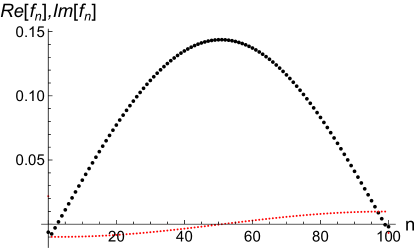
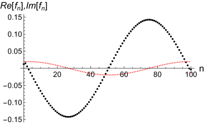
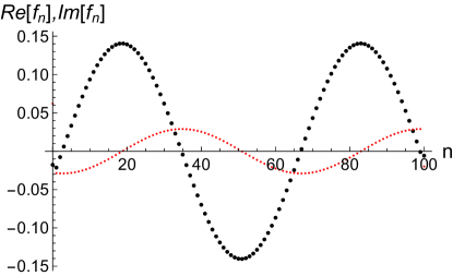
Figure 2: Amplitudes of the Bethe vectors $f_{n}$ in the expansion $\langle\Psi|=\sum_{n=0}^{N}\langle n|f_{n}$ for selected states in the single particle multiplet Fig. 1, obtained by numerical solutions of BAE (56). Top three panels in the left column: Phantom Bethe states with the three lowest energies $E_{j}$ of the single particle multiplet, (the energy increases from top to bottom). The thin lines connecting the points are guides for the eye. We show only ${\rm Re}[f_{n}]$ in the graphs. ${\rm Im}[f_{n}]$ looks similar, with a shift by a quarter of a period as in the right panel. Top three panels in the right column: Phantom Bethe states with the three highest energies $E_{j}$ of the real ${p_{j}}$ solutions (the energy decreases from top to bottom). Large and small points correspond to ${\rm Re}[f_{n}]$ and ${\rm Im}[f_{n}]$ respectively. Bottom row: Two phantom Bethe states corresponding to the two highest energy levels in the single particle multiplet, corresponding to imaginary ${p_{j}}$ solutions. The largest (the second largest) energy of the single particle multiplet corresponds to the right (left) Panel in the bottom row.

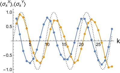
Figure 3: Transversal components of the magnetization profiles $\langle\sigma_{k}^{x}\rangle,\langle\sigma_{k}^{y}\rangle$ (blue and yellow curves, respectively), for a typical phantom Bethe state from $G_{1}^{+}$ (one regular Bethe root), versus site number $k$. Parameters: $N=29$, $\eta=\mathrm{i}\gamma=\mathrm{i}\frac{103\pi}{493}$, $\Delta=\cos\frac{103\pi}{493}\approx 0.79$, $\alpha_{\pm}=-\eta,\,\,\,\beta_{\pm}=0,\,\,\,\theta_{-}=\mathrm{i}\pi,\ \theta_{+}=\mathrm{i}(\pi-\Phi)$, and $\Phi=(N-1)\gamma$. The energy of the chosen state is $E_{m}=-5.39$ and the corresponding current is $j_{z}=1.216$, close to the asymptotic SHS current $j_{SHS}\approx 1.22$. The dotted line shows the $y$-component of an “ideal chiral” SHS profile for the same value of the anisotropy and is given for comparison.

VIII Discussion

We have analyzed the integrable XXZ Heisenberg spin chain with open boundary conditions and have described a novel type of solutions to the Bethe Ansatz equations containing phantom (infinite) Bethe roots, as well as regular (finite) Bethe roots. These solutions appear under condition (17) which leads to a complete decoupling of the Bethe Ansatz equations for phantom and regular Bethe roots. Phantom Bethe roots do not contribute to the energy of the system, which in case of spin chains with periodic boundary condition leads to degeneracies of the energies PhantomShort which we refer to as phantom excitations.

Condition (17) has appeared in OffDiagonal03 ; Nepomechie2003 ; Rafael2003 ; Cao2013off as a technical condition for the applicability of a modified Algebraic Bethe Ansatz, based on special properties of Sklyanin’s $K$-matrices. In the present manuscript, we have unveiled its meaning as a condition for the splitting of the Hilbert space into two invariant chiral subspaces $G_{M}^{\pm}$. In addition, here we used phantom Bethe roots as a useful shortcut to obtain reduced BAEs (18), (21). The integer parameter $0\leq M<N$ entering (17) determines the dimensions of the invariant subspaces, $\dim G_{M}^{+}=\sum_{k=0}^{M}\binom{N}{k}$ and $\dim G_{M}^{-}=2^{N}-\dim G_{M}^{+}$.

The meaning of the key parameter $M$, and its dual $\widetilde{M}=N-M-1$, parametrizing the hyperplane (17) is twofold. On one hand, $M$ is the maximal number of kinks in the chiral basis vectors (30) of $G_{M}^{+}$. Analogously, $\widetilde{M}$ is the maximal number of kinks in the chiral basis vectors of $G_{M}^{-}$. On the other hand, the fulfillment of (17) entails a reduction of the number of regular Bethe roots from $N$ in the general “inhomogeneous” BAE to $M$ or $\widetilde{M}$ in the reduced sets of BAE. The solutions of the two BAE sets give all Bethe eigenstates, which necessarily possess chiral properties since the nature of the invariant subspaces is chiral.

Conversely, we understand condition (17) as a criterion for the occurrence of phantom Bethe roots PhantomShort among the $N$ initial Bethe roots: the phantom Bethe roots decouple from the general “inhomogeneous” BAE, leading to the two (dual) homogeneous BAE sets for $M$ or $\widetilde{M}$ regular Bethe roots. The BAE for the phantom Bethe roots are not trivially satisfied just by these roots lying at infinity. The equations require a specific arrangement of the roots in a string that is unrelated to the usual TBA strings.

The appearance of invariant subspaces and the splitting of the set of eigenvectors into blocks is sowewhat similar to the occurrence of invariant subspaces for the periodic XXZ spin chain with fixed values of magnetization. There are however crucial differences: in the periodic case there are $N+1$ blocks, with magnetizations $-N/2,-N/2+1,...,N/2$ and BAE with a number of Bethe roots specific for each block, ranging from 0 to $N/2$ for even $N$ and to $(N-1)/2$ for odd $N$.

In contrast, in the open XXZ model fulfilling (17) with $0\leq M<N$ all eigenstates split into just two blocks, with basis vectors that are chiral, which leads to two sets of BAE with a total number of $M$ roots or $\widetilde{M}$ roots. The latter fact leads to highly unusual properties of the respective eigenstates such as high magnetization currents and quasiperiodic magnetization profiles.

The main result of this paper is the proof that in the open integrable XXZ spin chain, the occurrence of phantom Bethe roots entails the splitting of the Hilbert space into two chiral invariant subspaces. Based on the splitting, we are able to construct explicit Bethe vectors, the eigenstates of the open XXZ model with fine-tuned non-diagonal boundary fields, and investigate their properties to the same degree of detail as for the periodic spin chain with $U(1)$ symmetry for a given magnetization sector. The phantom Bethe eigenstates in open systems are very unusual and carry distinct chiral properties. This is due to the underlying chiral nature of the basis states, constituting the respective invariant subspaces. Our results can be used for the generation of stable spin helix states in experimental setups allowing to realize a paradigmatic XXZ model with tunable anisotropy 2020NatureSpinHelix as argued in PhantomShort .

It would be interesting to extend our results to other integrable systems with phantom Bethe roots e.g. to the spin-1 Fateev-Zamolodchikov model with open boundary conditions, see PhantomShort .

IX acknowledgments

Financial support from the Deutsche Forschungsgemeinschaft through DFG project KL 645/20-1, is gratefully acknowledged. Xin Zhang thanks the Alexander von Humboldt Foundation for financial support. Xin Zhang would like to thank Yupeng Wang and Junpeng Cao for discussions.

Appendix A Proof of Completeness

Here we prove that the basis of states spanning $G_{M}^{+}$ and $G_{M}^{-}$ is complete, i.e.

$${\cal H}=G_{M}^{+}\oplus G_{M}^{-}.$$ (73)

where ${\cal H}$ is the full Hilbert space. First we prove, that the vectors $\langle\,{g_{+,k}}|\in G_{M}^{+}$, $k=1,2,\ldots,\dim G_{M}^{+}$ are all independent for $\eta\neq 0,\mathrm{i}\pi$ (for the cases $\eta=0,\mathrm{i}\pi$, a jump $\phi_{n}(x)\rightarrow\phi_{n}(x+1)\equiv\phi_{n}(x)$ is trivial). We restrict our proof to the most “unfavourable”, extreme case of $\eta=\mathrm{i}\pi/2$, $\beta_{-}=0$ under the hermiticity condition (23). For this special case, the property $\phi_{n}(x)\phi_{n}^{\dagger}(x+1)\!=\!0$ renders all states $\langle\,g_{+,k}|\in G_{M}^{+}$ being pairwise orthonormal, $\left\langle\,g_{+,k}|g_{+,l}\right\rangle=2^{N}\delta_{kl}\left\langle\,g_{+,k}|g_{+,k}\right\rangle$. Thus, even in the most “unfavourable” setting all $\langle\,g_{+,k}|$ are independent, and the same is valid for the basis vectors $|{g_{-,k}}\rangle\!\rangle$ spanning $G_{M}^{-}$.

In the next step, we return to the general setup and show that any two vectors $g_{-}\in G_{M}^{-}$ and $g_{+}\in G_{M}^{+}$ are orthogonal. Define the function $y(n,j_{n},k_{n})$ as

$$\phi_{n}(j_{n})\,\tilde{\phi}_{n}(k_{n})=1-\mathsf{e}^{2y(n,j_{n},k_{n})\eta},\quad y(n,j_{n},k_{n})\!=\!j_{n}+k_{n}-n+1.$$ (74)

When $y(n,j_{n},k_{n})=0$, the local vectors $\phi_{n}(j_{n})$ and $\tilde{\phi}_{n}(k_{n})$ are orthogonal. From the definition of (30) and (31), any basis vector belonging to $G_{M}^{+}$ is a tensor product of $\phi_{n}(j_{n})$ with $0\leq j_{1}\leq j_{2}\ldots\leq j_{N}\leq M$ and any basis vector belonging to $G_{M}^{-}$ is a tensor product of $\tilde{\phi}_{n}(k_{n})$ with $0\leq k_{1}\leq k_{2}\ldots\leq k_{N}\leq\widetilde{M}$. It is easy to find

$$y(n+1,j_{n+1},k_{n+1})-y(n,j_{n},k_{n})=0,\pm 1,$$

$$y(N,j_{N},k_{N})\leq 0,\quad y(1,j_{1},k_{1})\geq 0.$$ (75)

so that $y(n,j_{n},k_{n})=0$ holds at least for one point $n$ ($1\leq n\leq N$). It shows that any pair of vectors $g_{-}\in G_{M}^{-}$ and $g_{+}\in G_{M}^{+}$ is orthogonal.

The dimension of $G_{M}^{+}$ is equal to the total number of different tuples $(n_{1},\ldots,n_{k})$ with $1\leq n_{1}<n_{2}<\ldots<n_{k}\leq N$ over all $k=0,\ldots M$, which is given by

$$\dim G_{M}^{+}=\sum_{m=0}^{M}\binom{N}{m}=\binom{N}{0}+\binom{N}{1}+\ldots\binom{N}{M}\,.$$ (76)

Analogously, the dimension of $G_{M}^{-}$ is

$$\dim G_{M}^{-}=\sum_{m=0}^{\widetilde{M}}\binom{N}{m}=\sum_{n=M+1}^{N}\binom{N}{n}\,.$$ (77)

The sum of dimensions $\dim G_{M}^{+}+\dim G_{M}^{-}=\sum_{n=0}^{N}\binom{N}{n}=2^{N}$ is identical to the dimension of the total Hilbert space ${\cal H}$. Hence the basis vectors in (30) and (31) span $G_{M}^{+}$ and $G_{M}^{-}$ respectively, hence (73) is proved.

Appendix B The invariance property of $G_{M}^{\pm}$

Here we prove the theorem for arbitrary Hamiltonian $H$ of type (1), satisfying (25), whether being hermitian or not. It is easy to prove that

$$\phi_{n}(x)\phi_{n+1}(x)h_{n,n+1}={\sinh}\eta\,\phi_{n}(x)\,\sigma_{n}^{z}\,\phi_{n+1}(x)-{\sinh}\eta\,\phi_{n}(x)\,\phi_{n+1}(x)\,\sigma_{n+1}^{z},$$ (78)

$$\phi_{n}(x\!-\!1)\phi_{n+1}(x)h_{n,n+1}={\sinh}\eta\,\phi_{n}(x\!-\!1)\,\phi_{n+1}(x)\,\sigma_{n+1}^{z}-{\sinh}\eta\,\phi_{n}(x\!-\!1)\,\sigma_{n}^{z}\,\phi_{n+1}(x),$$ (79)

$$\phi_{1}(x)h_{1}=-\frac{{\sinh}\eta\,{\cosh}(\alpha_{-}\!+\!\beta_{-}\!+\!2x\eta)}{{\sinh}(\alpha_{-}){\cosh}(\beta_{-})}\phi_{1}(x)$$

$$+\frac{{\sinh}\eta}{{\sinh}(\alpha_{-}){\cosh}(\beta_{-})}\left({\cosh}(\alpha_{-}){\sinh}(\beta_{-})-{\sinh}(\alpha_{-}\!+\!\beta_{-}\!+\!2x\eta)\right)\phi_{1}(x)\,\sigma_{1}^{z},$$ (80)

$$\phi_{N}(x)h_{N}=-\frac{{\sinh}\eta\,{\cosh}(\alpha_{+}\!+\!\beta_{+}\!+\!2(M\!-\!x)\eta)}{{\sinh}(\alpha_{+}){\cosh}(\beta_{+})}\phi_{N}(x)$$

$$+\frac{{\sinh}\eta}{{\sinh}(\alpha_{+}){\cosh}(\beta_{+})}({\sinh}(\alpha_{+}\!+\!\beta_{+}\!+\!2(M\!-\!x)\eta)-{\cosh}(\alpha_{+}){\sinh}(\beta_{+}))\phi_{N}(x)\,\sigma_{N}^{z}.$$ (81)

From (78) - (81), it is obvious that

$$\Phi_{+}(n_{1},\ldots,n_{k})\,H=C_{0}(n_{1},\ldots,n_{k})\Phi_{+}(n_{1},\ldots,n_{k})+\sum_{n=1}^{N}C_{n}(n_{1},\ldots,n_{k})\Phi_{+}(n_{1},\ldots,n_{k})\,\sigma_{n}^{z},$$ (82)

where $C_{n}(n_{1},\ldots,n_{k}),\,\,\,n=0,1,\ldots,N$, are some constants. Using Eqs. (78) - (81) repeatedly and checking the detailed coefficients, we can prove that the coefficient $C_{n}(n_{1},\ldots,n_{k})$ is zero when $\Phi_{+}(n_{1},\ldots,n_{k})$ has some special structure which is realized under any of the following conditions

$$\begin{aligned} &\Phi_{+}(n_{1},\ldots,n_{M})=\phi_{1}(0)\phi_{2}(0)\cdots,\,\,\mbox{i.e.}\,\,2\!\leq\!n_{1}\!<\!n_{2}\ldots\!<\!n_{M}\!\leq\!N,\qquad C_{1}(n_{1},\ldots,n_{M})=0,\\ &\Phi_{+}(n_{1},\ldots,n_{k})=\cdots\phi_{N-1}(M)\phi_{N}(M),\,\,\,\mbox{i.e.}\,\,1\!\leq\!n_{1}\!<\!n_{2}\ldots\!<\!n_{k}\!\leq\!N\!-\!2,\qquad\quad C_{N}(n_{1},\ldots,n_{k})=0,\\ &\Phi_{+}(n_{1},\ldots,n_{k})=\cdots\phi_{n-1}(x)\phi_{n}(x)\phi_{n+1}(x)\cdots,\,\,\mbox{i.e.}\,\,n_{m}\!\leq\!n\!-\!2,\,\,n_{m+1}\!\geq\!n\!+\!1,\!\quad C_{n}(n_{1},\ldots,n_{k})=0,\\ &\Phi_{+}(n_{1},\ldots,n_{k})=\cdots\phi_{n-1}(x-1)\phi_{n}(x)\phi_{n+1}(x+1)\cdots,\,\,\mbox{i.e.}\,\,n_{m}\!=\!n\!-\!1,\,\,n_{m+1}\!=\!n,\!\quad C_{n}(n_{1},\ldots,n_{k})=0.\end{aligned}$$ (83)

We have two useful identities

$$\begin{aligned} &\phi_{n}(x)\,\sigma_{n}^{z}=-\frac{{\cosh}\eta}{{\sinh}\eta}\phi_{n}(x)+\frac{\mathsf{e}^{\eta}}{{\sinh}\eta}\phi_{n}(x-1),\\ &\phi_{n}(x-1)\,\sigma_{n}^{z}=\frac{{\cosh}\eta}{{\sinh}\eta}\phi_{n}(x-1)-\frac{\mathsf{e}^{-\eta}}{{\sinh}\eta}\phi_{n}(x).\end{aligned}$$ (84)

Then, we obtain

$$\begin{aligned} &\phi_{n}(x-1)\phi_{n+1}(x)\sigma_{n}^{z}=\frac{{\cosh}\eta}{{\sinh}\eta}\phi_{n}(x-1)\phi_{n+1}(x)-\frac{\mathsf{e}^{-\eta}}{{\sinh}\eta}\phi_{n}(x)\phi_{n+1}(x),\\ &\phi_{n}(x)\phi_{n+1}(x)\sigma_{n}^{z}=-\frac{{\cosh}\eta}{{\sinh}\eta}\phi_{n}(x)\phi_{n+1}(x)+\frac{\mathsf{e}^{\eta}}{{\sinh}\eta}\phi_{n}(x-1)\phi_{n+1}(x),\\ &\phi_{n-1}(x)\phi_{n}(x+1)\sigma_{n}^{z}=-\frac{{\cosh}\eta}{{\sinh}\eta}\phi_{n-1}(x)\phi_{n}(x+1)+\frac{\mathsf{e}^{\eta}}{{\sinh}\eta}\phi_{n-1}(x)\phi_{n}(x),\\ &\phi_{n-1}(x)\phi_{n}(x)\sigma_{n}^{z}=\frac{{\cosh}\eta}{{\sinh}\eta}\phi_{n-1}(x)\phi_{n}(x)-\frac{\mathsf{e}^{-\eta}}{{\sinh}\eta}\phi_{n-1}(x)\phi_{n}(x+1).\end{aligned}$$ (85)

Let us extend the definition of $\Phi_{+}(n_{1},\ldots,n_{k})$ as

$$\Phi_{+}(0,n_{1},\ldots,n_{k})\equiv\Phi_{+}(n_{1},\ldots,n_{k}),\quad 1\leq n_{1}<\ldots<n_{k}\leq N.$$ (86)

Using Eqs. (82), (LABEL:psi;phi2) and the notation (86), we can prove that $\Phi_{+}(n_{1},\ldots,n_{k})\,H$ for $(n_{k-1},n_{k})\!\neq\!(N-1,N)$ is a linear combination of

$$\Phi_{+}(n_{1},\ldots,n_{k})\,\,\mbox{and}\,\,\,\Phi_{+}(n_{1},\ldots,n_{m}\pm 1,\ldots,n_{k}),\,\,m=1,\ldots,k.$$

Here the actions $\Phi_{+}(n_{1}\!=\!0,n_{2}\ldots,n_{k})H\!\to\!\Phi_{+}(n_{1}\!=\!1,n_{2}\ldots,n_{k})$ and $\Phi_{+}(n_{1}\!=\!1,n_{2}\ldots,n_{k})H\!\to\!\Phi_{+}(n_{1}\!=\!0,n_{2}\ldots,n_{k})$ represent the generation and annihilation of a kink at the left boundary respectively. Due to Eqs. (LABEL:C;property) and (LABEL:psi;phi2), the following unwanted structures will not appear

$$\Phi_{+}(\ldots,n_{j},n_{j+1}=n_{j},\,\ldots),$$

$$\Phi_{+}(n_{1},\ldots,n_{M+1}),\quad 1\leq n_{1}<n_{2}<\ldots<n_{M+1}\leq N.$$ (87)

In words, the Hamiltonian $H$ acting on $\Phi_{+}(n_{1},\ldots,n_{k})$ with $(n_{k-1},n_{k})\neq(N-1,N)$ can not degenerate any state beyond our basis vectors $\{\Phi_{+}(\ldots)\}$. Some nontrivial situations arise when $H$ acts on $\Phi_{+}(n_{1},\ldots,n_{k-1}\!=\!N\!-\!1,n_{k}\!=\!N)$

$$\Phi_{+}(\ldots,N\!-\!1,N)H=\cdots+F(\ldots,N\!-\!1,N)\,\Phi_{+}(\ldots,N,N),$$ (88)

where $\cdots$ on the RHS of (88) denotes a linear combination of some vectors belonging to $\Phi_{+}(\ldots)$ in (30) and $F(\ldots,N\!-\!1,N)$ is a constant. These “unwanted” vectors $\left\{\Phi_{+}(\ldots,N,N)\right\}$ are defined by replacing $\phi_{N-1}(M\!-\!2)\phi_{N}(M\!-\!1)$ in $\Phi_{+}(\ldots,N\!-\!1,N)$ with $\phi_{N-1}(M\!-\!2)\,\phi_{N}(M\!-\!2)$. In fact $\Phi_{+}(\ldots,N,N)$ is not an extra independent vector. Following the method in (74) and (75) we can prove $\Phi_{+}(\ldots,N,N)$ is orthogonal to all the basis vectors in $G_{M}^{-}$ and can be expanded in $G_{M}^{+}$ basis. Thus the invariance property of the subspace $G_{M}^{+}$ is proved. Analogously, we prove the invariance property of the set $G_{M}^{-}$.

Appendix C The proof of Eqs. (48)-(52)

Using Eqs. (78) - (81) and (LABEL:psi;phi), we find

$$\langle 0|H=\left(\frac{{\sinh}\eta\,{\cosh}(\alpha_{-}\!+\!\beta_{-})}{{\sinh}(\alpha_{-}){\cosh}(\beta_{-})}-\frac{{\sinh}\eta{\cosh}(\alpha_{+}\!+\!\beta_{+})}{{\sinh}(\alpha_{+}){\cosh}(\beta_{+})}\right)\langle 0|$$

$$\hskip 45.52458pt-\frac{2{\sinh}\eta\,{\cosh}(\alpha_{-}\!+\!\beta_{-}\!+\!\eta)}{{\sinh}(\alpha_{-}){\cosh}(\beta_{-})}\langle 1|,$$ (89)

$$\langle N|H=\left(\frac{{\sinh}\eta\,{\cosh}(\alpha_{+}\!+\!\beta_{+})}{{\sinh}(\alpha_{+}){\cosh}(\beta_{+})}-\frac{{\sinh}\eta\,{\cosh}(\alpha_{-}\!+\!\beta_{-})}{{\sinh}(\alpha_{-}){\cosh}(\beta_{-})}\right)\langle N|$$

$$\hskip 45.52458pt-\frac{2{\sinh}\eta\,{\cosh}(\alpha_{+}\!+\!\beta_{+}\!+\!\eta)}{{\sinh}(\alpha_{+}){\cosh}(\beta_{+})}\langle N\!-\!1|,$$ (90)

$$\langle n|H=-\left(\frac{{\sinh}\eta{\cosh}(\alpha_{-}\!+\!\beta_{-})}{{\sinh}(\alpha_{-}){\cosh}(\beta_{-})}+\frac{{\sinh}\eta{\cosh}(\alpha_{+}\!+\!\beta_{+})}{{\sinh}(\alpha_{+}){\cosh}(\beta_{+})}+{4{\cosh}\eta}\right)\langle n|$$

$$\qquad\qquad+2\langle n\!-\!1|+2\langle n\!+\!1|,\quad n=2,\ldots,N.$$ (91)

We have two useful identities

$$\frac{{\sinh}\eta\,{\cosh}(\alpha_{\pm}+\beta_{\pm})}{{\sinh}(\alpha_{\pm})\,{\cosh}(\beta_{\pm})}={a_{\pm}+b_{\pm}}-2{\cosh}\eta,$$ (92)

$$\frac{{\sinh}\eta\,{\cosh}(\alpha_{\pm}+\beta_{\pm}+\eta)}{{\sinh}(\alpha_{\pm})\,{\cosh}(\beta_{\pm})}={a_{\pm}\,b_{\pm}-1}.$$ (93)

where $a_{\pm},b_{\pm}$ are given by (37). Using Eqs. (92), (93), we can rewrite Eqs. (89) - (91) in terms of $a_{\pm}$ and $b_{\pm}$ and then easily obtain Eqs. (48) - (52).

Appendix D The solutions of BAE (36) with $M=1$

Recall the BAE for the $M=1$ case

$$\mathsf{e}^{2\mathrm{i}N{\mathrm{p}}}\prod_{\sigma=\pm}\frac{a_{\sigma}-\,\mathsf{e}^{\mathrm{i}{\mathrm{p}}}}{1-a_{\sigma}\,\mathsf{e}^{\mathrm{i}{\mathrm{p}}}}\,\,\frac{b_{\sigma}-\,\mathsf{e}^{\mathrm{i}{\mathrm{p}}}}{1-b_{\sigma}\,\mathsf{e}^{\mathrm{i}{\mathrm{p}}}}=1.$$ (94)

When $M=1$, we can treat $\mathsf{e}^{\mathrm{i}{\mathrm{p}}}$ as an unknown parameter which satisfies the unary equation (94) with degree $2N\!+\!4$. It is easy to prove that $\mathsf{e}^{\mathrm{i}{\mathrm{p}}}\!=\!\pm 1$ are always two trivial solutions. Replacing $\mathsf{e}^{\mathrm{i}{\mathrm{p}}}$ with $\mathsf{e}^{-\mathrm{i}{\mathrm{p}}}$, the BAE still holds which implies that $\mathsf{e}^{\mathrm{i}{\mathrm{p}}}$ and $\mathsf{e}^{-\mathrm{i}{\mathrm{p}}}$ are equivalent (see Eq. (39)). So we can summarize that the BAE (94) has $N\!+\!1$ independent valid solutions. If the Hamiltonian $H$ is hermitian, $\mathrm{p}$ can be a real or purely imaginary number. Here we only consider the easy plane regime case with (23).

Imaginary solutions

Introduce the following auxiliary function

$$Y(x)=x^{2N}\prod_{\sigma=\pm}\left(x-a_{\sigma}\right)\left(x-b_{\sigma}\right)-\prod_{\sigma=\pm}\left(1-a_{\sigma}\,x\right)\left(1\!-b_{\sigma}\,x\right).$$ (95)

The zero points of $Y(x)$ correspond to the solution of BAE (94). Suppose $0<a_{-}<1<a_{+}$. We find that

$$Y(1)=0,\quad Y(0)=-1,\quad Y\left(a_{+}^{-1}\right)=a_{+}^{-2N-4}\prod_{\sigma=\pm}(1-a_{+}\,a_{\sigma})(1-a_{+}\,b_{\sigma}).$$ (96)

When $a_{+}\,a_{-}>1$, we find $Y\left(a_{+}^{-1}\right)>0$ and equation $Y(x)=0$ has a solution in the interval $\left(0,\,a_{+}^{-1}\right)$. When $a_{+}\,a_{-}<1$, we consider the derivative of $Y(x)$ at the point $x=1$

$$Y^{\prime}(1)=\left(\prod_{\sigma=\pm}\left(1-a_{\sigma}\right)\left(1\!-b_{\sigma}\right)\right)\left(2N-\sum_{\sigma=\pm}\frac{a_{\sigma}+1}{a_{\sigma}-1}-\sum_{\sigma=\pm}\frac{b_{\sigma}+1}{b_{\sigma}-1}\right).\qquad\quad$$ (97)

If $Y^{\prime}(1)<0$, i.e.

$$N\!>\!\frac{1}{2}\left(\sum_{\sigma=\pm}\frac{a_{\sigma}+1}{a_{\sigma}-1}+\sum_{\sigma=\pm}\frac{b_{\sigma}+1}{b_{\sigma}-1}\right),$$ (98)

the function $Y(x)$ has a zero in the interval $\left(a_{+}^{-1},\,1\right)$.

Then suppose that $1<a_{-}<a_{+}$. We can prove that

$$Y(0)<0,\quad Y\left(a_{+}^{-1}\right)>0,\quad Y\left(a_{-}^{-1}\right)>0,\quad Y(1)=0.$$ (99)

Obviously, there exists a real solution in the interval $\left(0,\,a_{+}^{-1}\right)$. If $Y^{\prime}(1)>0$, i.e. the inequality (98) holds, there will be another real solution in the interval $\left(a_{-}^{-1},\,1\right)$. When $N\gg 1$ the purely imaginary solutions of (94) are very simple. We find

$$\mathsf{e}^{2\mathrm{i}N{\mathrm{p}}}\to\begin{cases}0,&-1<\mathsf{e}^{\mathrm{i}\mathrm{p}}<1,\\ \infty,&\mathsf{e}^{\mathrm{i}\mathrm{p}}<-1\,\,{\mbox{or}}\,\,\mathsf{e}^{\mathrm{i}\mathrm{p}}>1.\end{cases}$$

So there should be a purely imaginary solution at the point $\mathsf{e}^{\mathrm{i}\mathrm{p}}\!=\!{a_{\sigma}^{-1}}+O\left(\frac{1}{N}\right)$ in case of $a_{\sigma}>1$ or $a_{\sigma}<-1$. We can use a similar method to analyze the distribution of real solutions in other cases.

Real solutions

Suppose that $\mathrm{p}$ is a real number $\mathrm{p}=\epsilon$ with $\epsilon$ being a small positive real number, then we can prove

$$\frac{a_{\sigma}-\,\mathsf{e}^{\mathrm{i}{\mathrm{p}}}}{1-a_{\sigma}\,\mathsf{e}^{\mathrm{i}{\mathrm{p}}}}=\frac{a_{\sigma}-(1\!+\!\mathrm{i}\epsilon\!+\!\cdots)}{1-a_{\sigma}(1\!+\!\mathrm{i}\epsilon\!+\!\cdots)}=-1+\mathrm{i}\frac{a_{\sigma}+1}{a_{\sigma}-1}\epsilon+\cdots,\quad$$ (100)

with $\left|\frac{\mathrm{i}\epsilon}{1-a_{\sigma}}\right|\!\ll\!1$. If

$$\left|\frac{\mathrm{i}\epsilon}{1-a_{\sigma}}\right|\!\ll\!1,\,\,\,\left|\frac{\mathrm{i}\epsilon}{1-b_{\sigma}}\right|\!\ll\!1,\quad\sigma\!=\!\pm,$$

$\mathrm{p}=\epsilon=\frac{m\pi}{N}+O\left(\frac{1}{N^{2}}\right)$ is a solution of BAE (94) provided that $0\!<\!\frac{m}{N}\!\ll\!1$.

Now we suppose that $\mathrm{p}$ is a real number $\mathrm{p}=\pi-\epsilon$ with $\epsilon$ being a small positive real number, then we find

$$\frac{a_{\sigma}-\,\mathsf{e}^{\mathrm{i}{\mathrm{p}}}}{1-a_{\sigma}\,\mathsf{e}^{\mathrm{i}{\mathrm{p}}}}=\frac{a_{\sigma}+(1\!-\!\mathrm{i}\epsilon\!+\!\cdots)}{1+a_{\sigma}(1\!-\!\mathrm{i}\epsilon\!+\!\cdots)}=1+\mathrm{i}\frac{a_{\sigma}-1}{a_{\sigma}+1}\epsilon+\cdots,$$ (101)

with $\left|\frac{\mathrm{i}\epsilon}{1+a_{\sigma}}\right|\!\ll\!1$. If

$$\left|\frac{\mathrm{i}\epsilon}{1+a_{\sigma}}\right|\!\ll\!1,\,\,\,\left|\frac{\mathrm{i}\epsilon}{1+b_{\sigma}}\right|\!\ll\!1,\quad\sigma\!=\!\pm,$$

$\mathrm{p}=\pi-\epsilon=\pi-\frac{\pi m}{N}+O\left(\frac{1}{N^{2}}\right)$ is a solution of BAE (94) provided that $0\!<\frac{m}{N}\!\ll\!1$.

Let ${\mathrm{p}}=-\mathrm{i}\eta=\gamma$, the LHS of (94) thus becomes $\mathsf{e}^{2N\eta-4\eta-2\alpha_{+}-2\alpha_{-}}$. Obviously, ${\mathrm{p}}=\gamma$ is not a solution in the general case. However, in the thermodynamic limit $N\to\infty$, we can always find an integer $m$ to ensure

$$\eta=\frac{\mathrm{i}\pi m+\alpha_{+}+\alpha_{-}}{N-2}+O\left(\frac{1}{N}\right),\quad N\to\infty,\,\,\,m\to\infty.$$ (102)

So ${\mathrm{p}}=\gamma+O\left(\frac{1}{N}\right)$ becomes a solution of $(\ref{BAE_M1})$ in the thermodynamic limit.

Appendix E $M=1$ current: General case

Consider a hermitian Hamiltonian in the easy plane regime (23) with $\alpha_{\pm}$, $\theta_{\pm}$ and $\eta=\mathrm{i}\gamma$ being purely imaginary and $\beta_{+}=-\beta_{-}$ being real. The norm of the eigenvector $\langle\Psi|$ is

$$\langle\Psi|\Psi\rangle=\left(1+\mathsf{e}^{-2\beta_{+}}\right)^{N}\left(\sum_{n\leq m}\left(f_{n}\,f^{\ast}_{m}\,\tilde{b}_{+}^{m-n}+f_{n}^{\ast}\,f_{m}\,b_{+}^{m-n}\right)-\sum_{n}f_{n}\,f^{\ast}_{n}\right),$$ (103)

where $f^{\ast}_{n}$ is the complex conjugate of $f_{n}$ and $b_{+}(x)$ and $\tilde{b}_{+}(x)$ are defined in (37) and (41) respectively. Then, the current can be obtained by

$${j}^{z}=\frac{\langle\Psi|\,\mathbf{j}_{l}^{z}|\Psi\rangle}{\langle\Psi|\Psi\rangle} =\frac{2\sin\gamma}{{\cosh}^{2}(\beta_{+})\langle\Psi|\Psi\rangle}\left(-\sum_{n=0}^{N}f_{n}f^{\ast}_{n}+\sum_{\begin{subarray}{c}n_{1}\leq n_{2}<l\\ l<n_{1}\leq n_{2}\end{subarray}}\left(f_{n_{1}}\,f^{\ast}_{n_{2}}\,\tilde{b}_{+}^{n_{2}-n_{1}}+f^{\ast}_{n_{1}}\,f_{n_{2}}\,b_{+}^{n_{2}-n_{1}}\right)\right.$$

$$\quad\left.+\sum_{n_{1}<l<n_{2}}\left(f_{n_{1}}\,f^{\ast}_{n_{2}}\,\tilde{b}_{+}^{n_{2}-n_{1}-2}+f^{\ast}_{n_{1}}\,f_{n_{2}}\,b_{+}^{n_{2}-n_{1}-2}\right)\right).$$ (104)

The current is independent of the site number. For a hermitian Hamiltonian, the parameter ${\mathrm{p}}$ should be real or purely imaginary. If $\mathrm{p}$ is real for large $N$, the norm is order $O(N)$ and we obtain the expression of the current in the leading approximation as

$$j^{z}=\frac{2\sin\gamma}{{\cosh}^{2}(\beta_{+})}\left(1-O\left(\frac{1}{N}\right)\right).$$ (105)

If ${\mathrm{p}}$ is purely imaginary, the norm is order $O(\mathsf{e}^{2N\left|\mathrm{p}\right|})$ and the current is

$$j^{z}=\frac{2\,\sin\gamma}{{\cosh}^{2}(\beta_{+})}\left(1-O\left(\mathsf{e}^{-N\left|\mathrm{p}\right|}\right)\right).$$ (106)

References

• (1) N. Jepsen, J. Amato-Grill, I. Dimitrova, W. W. Ho, E. Demler, W. Ketterle. Spin transport in a tunable Heisenberg model realized with ultracold atoms. Nature 588, 403 (2020).
• (2) M. Gaudin. The Bethe Wavefunction (Cambridge University Press, 2014).
• (3) T. Prosen, E. Ilievski. Families of quasilocal conservation laws and quantum spin transport. Phys. Rev. Lett. 111, 057203 (2013).
• (4) F. Göhmann, A. Klümper, A. Seel. Integral representations for correlation functions of the XXZ chain at finite temperature. J. Phys. A: Math. Gen. 37, 7625 (2004).
• (5) H. E. Boos, F. Göhmann, A. Klümper, J. Suzuki. Factorization of multiple integrals representing the density matrix of a finite segment of the Heisenberg spin chain. J. Stat. Mech. P04001 (2006).
• (6) B. Bertini, F. Heidrich-Meisner, C. Karrasch, T. Prosen, R. Steinigeweg, M. Znidaric. Finite-temperature transport in one-dimensional quantum lattice models. eprint arXiv:2003.03334.
• (7) V. Popkov, X. Zhang, A. Klümper. Phantom Bethe excitations and spin helix eigenstates in integrable periodic and open spin chains. eprint arXiv:2102.03295.
• (8) Y. Wang, W.-L. Yang, J. Cao, K. Shi. Off-Diagonal Bethe Ansatz for Exactly Solvable Models (Springer, 2015).
• (9) J. Cao, W.-L. Yang, K. Shi, Y. Wang. Off-diagonal Bethe ansatz solutions of the anisotropic spin-1/2 chains with arbitrary boundary fields. Nucl. Phys. B 877, 152 (2013).
• (10) X. Zhang, Y.-Y. Li, J. Cao, W.-L. Yang, K. Shi, Y. Wang. Bethe states of the XXZ spin-1/2 chain with arbitrary boundary fields. Nucl. Phys. B 893, 70 (2015).
• (11) G. Niccoli. Non-diagonal open spin-1/2 XXZ quantum chains by separation of variables: complete spectrum and matrix elements of some quasi-local operators. J. Stat. Mech. P10025 (2012).
• (12) S. Faldella, N. Kitanine, G. Niccoli. The complete spectrum and scalar products for the open spin-1/2 XXZ quantum chains with non-diagonal boundary terms. J. Stat. Mech. P01011 (2014).
• (13) N. Kitanine, J. M. Maillet, G. Niccoli. Open spin chains with generic integrable boundaries: Baxter equation and Bethe ansatz completeness from separation of variables. J. Stat. Mech. P05015 (2014).
• (14) J. Cao, H.-Q. Lin, K.-J. Shi, Y. Wang. Exact solution of XXZ spin chain with unparallel boundary fields. Nucl. Phys. B 663, 487 (2003).
• (15) S. Belliard, R. Pimenta. Modified algebraic Bethe ansatz for XXZ chain on the segment – II – general cases. Nucl. Phys. B 894, 527 (2015).
• (16) R. I. Nepomechie, F. Ravanini. Completeness of the Bethe Ansatz solution of the open XXZ chain with nondiagonal boundary terms. J. Phys. A: Math. Gen. 36, 11391 (2003).
• (17) R. I. Nepomechie. Bethe ansatz solution of the open XXZ chain with nondiagonal boundary terms. J. Phys. A: Math. Gen. 37, 433 (2003).
• (18) R. I. Nepomechie. Functional relations and Bethe Ansatz for the XXZ chain. J. Stat. Phys. 111, 1363 (2003).
• (19) S. Hild, T. Fukuhara, P. Schauß, J. Zeiher, M. Knap, E. Demler, I. Bloch, C. Gross. Far-from-equilibrium spin transport in heisenberg quantum magnets. Phys. Rev. Lett. 113, 147205 (2014).
• (20) V. Popkov, C. Presilla. Obtaining pure steady states in nonequilibrium quantum systems with strong dissipative couplings. Phys. Rev. A 93, 022111 (2016).
• (21) V. Popkov, G. M. Schütz. Solution of the Lindblad equation for spin helix states. Phys. Rev. E 95, 042128 (2017).
• (22) V. Popkov, T. Prosen, L. Zadnik. Exact Nonequilibrium Steady State of Open XXZ/XYZ Spin-1/2 Chain with Dirichlet Boundary Conditions. Phys. Rev. Lett. 124, 160403 (2020).
• (23) V. Popkov, T. Prosen, L. Zadnik. Inhomogeneous matrix product ansatz and exact steady states of boundary-driven spin chains at large dissipation. Phys. Rev. E 101, 042122 (2020).