Multi-Sample Online Learning for Spiking Neural Networks based on Generalized Expectation Maximization
Abstract
Spiking Neural Networks (SNNs) offer a novel computational paradigm that captures some of the efficiency of biological brains by processing through binary neural dynamic activations. Probabilistic SNN models are typically trained to maximize the likelihood of the desired outputs by using unbiased estimates of the log-likelihood gradients. While prior work used single-sample estimators obtained from a single run of the network, this paper proposes to leverage multiple compartments that sample independent spiking signals while sharing synaptic weights. The key idea is to use these signals to obtain more accurate statistical estimates of the log-likelihood training criterion, as well as of its gradient. The approach is based on generalized expectation-maximization (GEM), which optimizes a tighter approximation of the log-likelihood using importance sampling. The derived online learning algorithm implements a three-factor rule with global per-compartment learning signals. Experimental results on a classification task on the neuromorphic MNIST-DVS data set demonstrate significant improvements in terms of log-likelihood, accuracy, and calibration when increasing the number of compartments used for training and inference.
Index Terms— Spiking Neural Networks, Variational Learning, Expectation Maximization, Neuromorphic Computing.
1 Introduction
Many of the recent breakthroughs towards solving complex tasks have relied on learning and inference algorithms for Artificial Neural Networks (ANNs) that have prohibitive energy and time consumption for implementation on battery-powered devices [1, 2]. This has motivated a renewed interest in exploring the use of Spiking Neural Networks (SNNs) to capture some of the efficiency of biological brains for information encoding and processing [3]. Experimental evidence has confirmed the potential of SNNs in yielding energy consumption savings as compared to ANNs in many tasks of interest, such as keyword spotting [4], while also demonstrating computational advantages in dynamic environments [5].
Inspired by biological brains, SNNs consist of neural units that process and communicate over recurrent computing graphs via sparse binary spiking signals over time, rather than via real numbers [6]. Spiking neurons store and update a state variable, the membrane potential, that evolves over time as a function of past spike signals from pre-synaptic neurons. Most implementations are based on deterministic spiking neurons that spike when the membrane potential crosses a threshold. These models can be trained via various approximations of back-propagation through time (BPTT). The approximations aim at dealing with the non-differentiability of the threshold function, and at reducing the complexity of BPTT, making it possible to implement local update rules that do not require global backpropagation paths through the computation graph.
As an alternative, probabilistic spiking neural models based on the generalized linear model (GLM) for spiking neurons can be trained by directly maximizing a lower bound on the likelihood of the SNN producing desired outputs [7, 8, 9, 10]. This maximization over the synaptic weights typically uses an unbiased estimate of the gradient of the log-likelihood that leverages a single sample from the output of the neurons. The resulting learning algorithm implements an online learning rule that is local apart from a global learning signal.
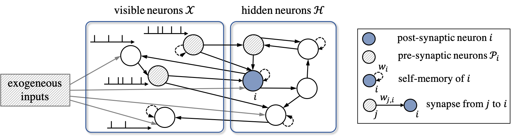
In this paper, as illustrated in Fig. 1, we explore a more general SNN model in which each spiking neuron has multiple compartments. Each compartment tracks a distinct membrane potential, with all compartments sharing the same synaptic weights. This architecture would provide no benefits with deterministic models, since all compartments would produce the same outputs. This is not the case under probabilistic neural models when the compartments use independent random number generators to generate spikes. The independent spiking outputs across the compartments can be leveraged in two ways: (i) during inference, the multiple outputs can be used to robustify the decision and to quantify uncertainty; and (ii) during training, these signals evaluate a more accurate estimate of the log-likelihood learning criterion and of the corresponding gradient. In this paper, we propose a multi-sample online learning rule that leverages a multi-compartment probabilistic SNN model. The proposed approach adopts generalized expectation-maximization (GEM) [11, 12, 13, 14], and it uses multiple samples drawn independently from the compartments to approximate the log-likelihood bound via importance sampling. This yields a better statistical estimate of the log-likelihood and of its gradient as compared to conventional single-sample estimators. Experimental results on a neuromorphic data set demonstrate the advantage of leveraging multiple compartments in terms of accuracy and calibration [15].
2 Multi-Compartment SNN Model
A -compartment SNN model is defined as a network connecting a set of spiking neurons via an arbitrary directed graph, which may have cycles, with each neuron and synapse having compartments. As illustrated in Fig. 1, each neuron receives the signals emitted by the set of pre-synaptic neurons connected to it through directed links, known as synapses. Each th synaptic compartment for a synapse processes the output of the th compartment of pre-synaptic neuron ; and its output is in turn processed by the th compartment of the post-synaptic neuron , for .
Following a discrete-time implementation of the probabilistic generalized linear neural model (GLM) for spiking neurons [16, 9], at any time , the th compartment of spiking neuron outputs a binary value , with “” representing the emission of a spike, for . We collect in vector the spikes of the th compartment emitted by all neurons at time , and denote by the spike sequences of all neurons processed by the compartment up to time . Each post-synaptic neuron receives past input spike signals from the set of pre-synaptic neurons through the th compartment of synapses. With some abuse of notation, we include exogeneous inputs to a neuron in the set of pre-synaptic neurons, see Fig. 1.
For the th compartment, independently of the other compartments, the instantaneous spiking probability of neuron at time , conditioned on the value of the membrane potential, is defined as
| (1) |
where is the sigmoid function and the membrane potential summarizes the effect of the past spike signals from pre-synaptic neurons and of its past activity . Note that each compartment stores and updates a distinct membrane potential. From (1), the negative log-probability of the output corresponds to the binary cross-entropy loss
| (2) | ||||
| (3) |
The joint probability of the spike signals up to time is defined using the chain rule as , where is the model parameters, with being the local model parameters of neuron as detailed below.
The membrane potential is obtained as the output of spatio-temporal synaptic filter and somatic filter . Specifically, each synapse from a pre-synaptic neuron to a post-synaptic neuron computes the synaptic trace , while the somatic trace of neuron is computed as , where we denote by the convolution operator. The membrane potential of neuron at time is finally given as the weighted sum
| (4) |
where is a synaptic weight of the synapse ; is the self-memory weight; and is a bias, with the local model parameters being shared among all compartments of neuron .
3 Training
During training, the shared model parameters are adapted jointly across all compartments with the goal of maximizing the log-likelihood that a subset of “visible” neurons outputs desired spiking signals. The desired samples are specified by the training data as spiking sequences for some , in response to given exogeneous inputs. Mathematically, the maximum log-likelihood (ML) problem can be written as
| (5) |
where is the probability of the desired output for any of the compartments. To evaluate the log-likelihood , one needs to average over the spiking signals of “hidden”, or latent, neurons in the complement set .
In this section, we propose an online learning rule that leverages the available compartments by following the generalized expectation-maximization (GEM) introduced in [14]. Throughout the paper, we define the temporal average operator of a time sequence with some constant as with .
GEM-VLSNN: Generalized EM Variational online Learning for SNNs. Following the principles of GEM [11, 12, 13, 14], given the current iterate , we tackle the problem of minimizing at each time the following approximate upper bound on the objective in (5) [11, 9]
| (6) |
where is a discount factor and is the posterior distribution. The bound is exact for , and we have added the discounted average in (6) in order to obtain online rules. The posterior distribution is generally intractable, and, following [7, 8, 9], we approximate it with the “causally conditioned” distribution , where we have used the notation [17]
| (7) |
and we have denoted by and the collection of model parameters for visible and hidden neurons respectively. Then, following GEM, we use independent samples drawn from the distribution to carry out the marginalization via importance sampling. Accordingly, we approximate the loss function (6) as
| (8) | ||||
| (9) | ||||
| (10) | ||||
| (11) |
The approximate upper bound in (8) is obtained by approximating the importance weights of the samples as
| (12) | ||||
| (13) |
where in (a) we have used a Monte Carlo (MC) estimate with samples for ; and in (b) we have defined as the vector of log-probabilities of the samples at time by using temporal averaging operator as
| (14) |
with some constant , and have defined the SoftMax function as
| (15) |
We note that the resulting MC estimate can better capture the inherent uncertainty of the true posterior distribution more precisely with a larger .
An online local update rule, which we refer to as GEM Variational online Learning for SNNs (GEM-VLSNN), is obtained by minimizing in (8) via stochastic gradient descent in the direction of the negative gradient . This yields the update rule at time
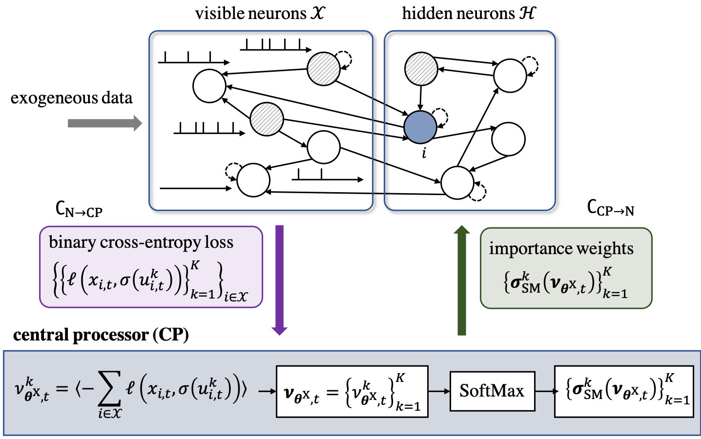
with a learning rate . As illustrated in Fig. 2, this rule can be implemented as follows. At each time , a central processor (CP) collects the binary cross-entropy values of all compartments from all visible neurons in order to compute the importance weights of the compartments as in (14), and it computes the normalized weights using the SoftMax function as in (15). Then, the SoftMax values are fed back from the CP to all neurons (both visible and hidden neurons). Finally, for each neuron , GEM-VLSNN updates the local model parameters as
| (16) | ||||
| (17) | ||||
| (18) |
where we have used standard expressions for the derivatives of the cross-entropy loss [9, 18], and we set for visible neuron and for hidden neuron .
Interpreting GEM-VLSNN. The update rule (16) follows a three-factor format in the sense that it can be written as [19]
| (19) |
where is the learning rate. The three-factor rule (19) sums the contributions from the compartments, with contribution of the th compartment depending on three factors: and respectively representing the activity of the pre-synaptic neuron and of the post-synaptic neuron processed by the compartment, and finally determines the sign and magnitude of the contribution of the compartment to the learning update. The update rule (19) is hence local, with the exception of the learning signal. Specifically, for each neuron , the gradients contain the post-synaptic error and post-synaptic somatic trace ; the pre-synaptic synaptic trace ; and the global learning signals . The importance weights computed using the SoftMax function can be interpreted as the common learning signals for all neurons, with the contribution of each compartment being weighted by . From (14)-(15), the importance weight measures the relative effectiveness of the random realization of the hidden neurons within the th compartment in reproducing the desired behavior of the visible neurons.
Communication Load. As discussed, GEM-VLSNN requires bi-directional communication. As seen in Fig. 2, at each time , unicast communication from neurons to CP is required in order to compute the importance weights by collecting information from all visible neurons. The resulting unicast communication load is real numbers. The importance weights are then sent back to all neurons, resulting a broadcast communication load from CP to neurons equal to real numbers. As GEM-VLSNN requires computation of importance weights at CP, the communication loads increase linearly to .
4 Experiments
In this section, we evaluate the performance of the proposed scheme GEM-VLSNN on classification task defined on the neuromorphic data set MNIST-DVS [20]. For each pixel of an image, binary spiking signals are recorded when the pixel’s luminosity changes by more than a given amount, and no event is recorded otherwise. As in [21, 22], images are cropped to pixels, and uniform downsampling over time is carried out to obtain time samples per each image. The training and test data set respectively contains and examples per each digit, from to . We focus on a classification task that classifies three digits , where the spiking signals encoding an MNIST-DVS image are given as exogeneous inputs. The digit labels are encoded by the neurons in the read-out layer, where the output neuron corresponding to the correct label is assigned a desired output spiking signal , while the other neurons are assigned for .
We consider a generic, non-optimized network architecture with a set of fully connected hidden neurons, all receiving the exogeneous inputs as pre-synaptic signals, and a read-out visible layer with neurons, directly receiving pre-synaptic signals from all exogeneous inputs and all hidden neurons without recurrent connections between visible neurons. For synaptic and somatic filters, we choose a set of three raised cosine functions with a synaptic duration of time steps, following the approach [16]. We train a -compartment SNN by varying the number , with the learning rate and time constants , which have been selected after a non-exhaustive manual search.
For testing, a -compartment SNN with the trained weights is used for inference. First, we measure the marginal log-likelihood for a desired output signal via the empirical average over independent realizations of the hidden neurons. Next, in order to evaluate the classification accuracy, we adopt a standard majority decoding rule: for each compartment , the output neuron with the largest number of output spikes for each is selected, obtaining the decision ; then the index of the output neuron that receives the most votes is set to the predicted class as , where is the number of votes for class . Finally, we consider calibration as a performance metric. To this end, the prediction probability , or confidence, of a decision is derived from the vote count variables using the SoftMax function, i.e., . The expected calibration error (ECE) measures the difference in expectation between confidence and accuracy, i.e.,
| (20) |
In (20), the probability is the probability that is the correct decision for inputs that yield accuracy . The ECE can be estimated by using quantization and empirical averages as detailed in [15].

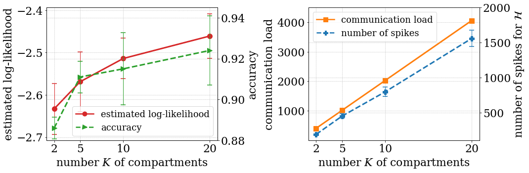
To start, we trained a -compartment SNN and tested the SNN with compartments for . We chose the model with the best performance on the test data set across the iterations, and the corresponding estimated log-likelihood and accuracy are illustrated as a function of in Fig. 3. It can be observed that using more compartments improves the testing performance due to the optimization of increasingly tighter bound on the training log-likelihood. Fig. 3 also shows the broadcast communication load from CP to neurons increases linearly with , with a larger implying a proportionally larger number of spikes emitted by the hidden neurons. The proposed GEM-VLSNN is seen to enable a flexible trade-off between communication load and energy consumption [23], on the one hand, and testing performance, on the other, by leveraging the availability of compartments.
We then plot in Fig. 4 the estimated log-likelihood, accuracy, and ECE (20) of test data set as a function of the number of training iterations. An improved test log-likelihood due to a larger translates into a model that more accurately reproduces conditional probability of outputs given inputs [15, 24], which in turn enhances calibration. In contrast, accuracy can be improved with a larger but only if regularization via early stopping is carried out. This points to the fact that the goal of maximizing the likelihood of specific desired output spiking signals is not equivalent to maximizing the classification accuracy.
5 Conclusion
This paper has explored a probabilistic spiking neural model in which spiking neurons run multiple compartments, each generating independent spiking outputs, while sharing the same synaptic weights across compartments. We have proposed a novel multi-sample online learning algorithm for SNNs that leverages multiple compartments to obtain a better statistical estimate of the log-likelihood learning criterion and of its gradient. Experiments on a neuromorphic data set have demonstrated improvements of performance with increasing number of compartments in training and inference. As future work, the proposed learning algorithm can be extended to learning tasks with other reward functions instead of log-likelihood, such as Van Rossum distance [10, 25], or to networks of spiking Winner-Take-All (WTA) circuits [26, 27], which process multi-valued spikes.
References
- [1] Karen Hao, “Training a single AI model can emit as much carbon as five cars in their lifetimes,” MIT Technology Review, 2019.
- [2] Emma Strubell, Ananya Ganesh, and Andrew McCallum, “Energy and policy considerations for deep learning in NLP,” arXiv preprint arXiv:1906.02243, 2019.
- [3] Carver Mead, “Neuromorphic electronic systems,” Proceedings of the IEEE, vol. 78, no. 10, pp. 1629–1636, 1990.
- [4] Peter Blouw et al., “Benchmarking keyword spotting efficiency on neuromorphic hardware,” in Proc. of Annual Neuro-inspired Computational Elements Workshop, 2019, pp. 1–8.
- [5] Abu Sebastian, Manuel Le Gallo, Riduan Khaddam-Aljameh, and Evangelos Eleftheriou, “Memory devices and applications for in-memory computing,” Nature Nanotechnology, pp. 1–16, 2020.
- [6] Emre O Neftci, Hesham Mostafa, and Friedemann Zenke, “Surrogate gradient learning in spiking neural networks: Bringing the power of gradient-based optimization to spiking neural networks,” IEEE Signal Processing Magazine, vol. 36, no. 6, pp. 51–63, 2019.
- [7] D Rezende Jimenez et al., “Stochastic variational learning in recurrent spiking networks.,” Frontiers in Computational Neuroscience, vol. 8, pp. 38–38, 2014.
- [8] Johanni Brea, Walter Senn, and Jean-Pascal Pfister, “Matching recall and storage in sequence learning with spiking neural networks,” Journal of Neuroscience, vol. 33, no. 23, pp. 9565–9575, 2013.
- [9] Hyeryung Jang et al., “An introduction to probabilistic spiking neural networks: Probabilistic models, learning rules, and applications,” IEEE Signal Processing Magazine, vol. 36, no. 6, pp. 64–77, 2019.
- [10] Friedemann Zenke and Surya Ganguli, “Superspike: Supervised learning in multilayer spiking neural networks,” Neural Computation, vol. 30, no. 6, pp. 1514–1541, 2018.
- [11] Christopher M Bishop, Pattern recognition and machine learning, Springer, 2006.
- [12] Osvaldo Simeone, “A brief introduction to machine learning for engineers,” Foundations and Trends® in Signal Processing, vol. 12, no. 3-4, pp. 200–431, 2018.
- [13] Radford M Neal and Geoffrey E Hinton, “A view of the EM algorithm that justifies incremental, sparse, and other variants,” in Learning in graphical models, pp. 355–368. Springer, 1998.
- [14] Yichuan Tang and Ruslan R Salakhutdinov, “Learning stochastic feedforward neural networks,” in Proc. of Advances in Neural Information Processing Systems, 2013, pp. 530–538.
- [15] Chuan Guo et al., “On calibration of modern neural networks,” arXiv preprint arXiv:1706.04599, 2017.
- [16] Jonathan W Pillow et al., “Spatio-temporal correlations and visual signalling in a complete neuronal population,” Nature, vol. 454, no. 7207, pp. 995–999, 2008.
- [17] Gerhard Kramer, Directed information for channels with feedback, Hartung-Gorre, 1998.
- [18] Hyeryung Jang and Osvaldo Simeone, “Training dynamic exponential family models with causal and lateral dependencies for generalized neuromorphic computing,” in Proc. of International Conference on Acoustics, Speech and Signal Processing. IEEE, 2019, pp. 3382–3386.
- [19] Nicolas Frémaux and Wulfram Gerstner, “Neuromodulated spike-timing-dependent plasticity, and theory of three-factor learning rules,” Frontiers in Neural Circuits, vol. 9, pp. 85, 2016.
- [20] Teresa Serrano-Gotarredona and Bernabé Linares-Barranco, “Poker-DVS and MNIST-DVS. their history, how they were made, and other details,” Frontiers in Neuroscience, vol. 9, pp. 481, 2015.
- [21] Bo Zhao et al., “Feedforward categorization on aer motion events using cortex-like features in a spiking neural network,” IEEE Transactions on Neural Networks and Learning Systems, vol. 26, no. 9, pp. 1963–1978, 2014.
- [22] James A Henderson, TingTing A Gibson, and Janet Wiles, “Spike event based learning in neural networks,” arXiv preprint arXiv:1502.05777, 2015.
- [23] Paul A Merolla et al., “A million spiking-neuron integrated circuit with a scalable communication network and interface,” Science, vol. 345, no. 6197, pp. 668–673, 2014.
- [24] Christopher M Bishop, “Mixture density networks,” 1994.
- [25] MCW van Rossum, “A novel spike distance,” Neural Computation, vol. 13, no. 4, pp. 751–763, 2001.
- [26] Hesham Mostafa and Gert Cauwenberghs, “A learning framework for Winner-Take-All networks with stochastic synapses,” Neural Computation, vol. 30, no. 6, pp. 1542–1572, 2018.
- [27] Hyeryung Jang, Nicolas Skatchkovsky, and Osvaldo Simeone, “VOWEL: A local online learning rule for recurrent networks of probabilistic spiking Winner-Take-All circuits,” arXiv preprint arXiv:2004.09416, 2020.