Estimating 2-Sinkhorn Divergence between Gaussian Processes from Finite-Dimensional Marginals

Abstract

Optimal Transport (OT) has emerged as an important computational tool in machine learning and computer vision, providing a geometrical framework for studying probability measures. OT unfortunately suffers from the curse of dimensionality and requires regularization for practical computations, of which the entropic regularization is a popular choice, which can be ’unbiased’, resulting in a Sinkhorn divergence. In this work, we study the convergence of estimating the 2-Sinkhorn divergence between Gaussian processes (GPs) using their finite-dimensional marginal distributions. We show almost sure convergence of the divergence when the marginals are sampled according to some base measure. Furthermore, we show that using $n$ marginals the estimation error of the divergence scales in a dimension-free way as $\mathcal{O}\left(\epsilon^{-1}n^{-\frac{1}{2}}\right)$, where $\epsilon$ is the magnitude of entropic regularization.

1 Introduction

Gaussian processes (GPs) are infinite-dimensional counterparts of normal distributions, which are plentiful in machine learning tasks where one aims to infer functional relationships with uncertainty estimates (Hauberg et al., 2015; Lê et al., 2015; Roberts et al., 2013). Centered GPs correspond to covariance operators, which appear as features in computer vision (Faraki et al., 2015; Harandi et al., 2014) and natural language processing (Pigoli et al., 2014). To compare such operators with each other requires defining a metric or a divergence. Such divergences exist readily for the finite-dimensional covariance matrices (Arsigny et al., 2006; Pennec et al., 2006), but these expressions do not always extend in a straight-forward manner to the infinite-dimensional setting, mainly due to the eigenvalues of covariance operators converging to zero (Minh et al., 2014; Minh, 2015). As the covariance operators correspond to centered probability measures, optimal transport (OT) can be applied to compute well-defined divergences.

OT (Villani, 2008; Peyré et al., 2019) provides a geometrical toolkit for studying the space of probability measures by extending a cost function between samples of the probabilities to a divergence between the entire probability measures. A special subclass of these divergences is formed by the Wasserstein metrics, which are proper metrics, and therefore enjoy favorable topological properties compared to information theoretical divergences, such as the Kullback-Leibler (KL) divergence. However, the OT problem requires regularization due to bad scaling properties with respect to the sample dimension, behaving as $\mathcal{O}\left(n^{-\frac{1}{d}}\right)$ (Dudley, 1969). To combat this, a popular approach is to combine OT and information theoretical divergences, by regularizing the OT problem with a divergence term (Dessein et al., 2018; Di Marino & Gerolin, 2020), e.g. the KL-divergence, resulting in entropy-regularized OT (Cuturi, 2013), improving the sample complexity to $\mathcal{O}\left((1+\epsilon^{-\lfloor d/2\rfloor})n^{-\frac{1}{2}}\right)$ (Genevay et al., 2019), which has been further sharpened to $\mathcal{O}\left(\epsilon\left(1+\frac{\sigma^{\lceil 5d/2\rceil+6}}{\epsilon^{\lceil 5d/4\rceil+3}}\right)n^{-\frac{1}{2}}\right)$ (Mena & Weed, 2019).

OT approaches to compute divergences between Gaussians have been studied extensively, as closed form expressions can be derived. The $2$-Wasserstein distance between normal distributions was studied in (Givens et al., 1984; Dowson & Landau, 1982; Olkin & Pukelsheim, 1982; Knott & Smith, 1984), $2$-Wasserstein distance between GPs in (Gelbrich, 1990; Mallasto & Feragen, 2017; Masarotto et al., 2019). Also the entropy-regularized $2$-Wasserstein distance and the Sinkhorn divergence between normal distributions have garnered considerable attention lately  (Mallasto et al., 2020; Janati et al., 2020; Gerolin et al., 2019; del Barrio & Loubes, 2020; Ripani, 2017), and their extensions to Gaussian measures and GPs (Minh, 2020).

In this work, we study the complexity of computing the entropy-regularized $2$-Wasserstein distance as well as the $2$-Sinkhorn divergence between two GPs using a finite amount of their marginals. In other words, the question is: given two GPs $f_{0},f_{1}$ over an index set $\mathcal{X}$, over how many samples $\{x_{1},...,x_{n}\}\subseteq\mathcal{X}$ should we evaluate the GPs to get a reasonable approximation for the $2$-Sinkhorn divergence with regularization $\epsilon$ between the GPs?

The contributions can be summarized as follows:

• We show that the entropy-regularized 2-Wasserstein distance has a marginal complexity (error rate as a function of marginals) of $\mathcal{O}\left(\frac{1}{\sqrt{n}}\left(\frac{1}{\epsilon}+\mathrm{const.}\right)\right)$ and the $2$-Sinkhorn divergence $\mathcal{O}\left(\frac{1}{\epsilon\sqrt{n}}\right)$.

• We provide concentration bounds for the errors of the empirical estimates for the two divergences.

• We illustrate empirically the convergence of the estimates, and observe that increasing $\epsilon$ does not necessarily increase estimation accuracy in terms of relative error as we increase $n$. However, if we increase the dimension of $\mathcal{X}$, larger $\epsilon$ also decreases relative error.

2 Background

In the following, we briefly summarize some prerequisites and fix notation.

2.1 Gaussian Processes and Covariance Operators

Gaussian processes.

A Gaussian process (GP) $f$ is a collection of random variables, such that any finite restriction $(f(x_{i}))_{i=1}^{n}$ has a joint Gaussian distribution, where $x_{i}\in\mathcal{X}$, and $(\mathcal{X},\rho)$ is the index set equipped with a probability measure $\rho$. We will assume $\mathcal{X}\subset\mathbb{R}^{d}$ to be compact. A GP is entirely characterized by the pair

$$m(x) =\mathbb{E}{f(x)},$$ (1)

$$K(x,x^{\prime}) =\mathbb{E}\left(f(x)-m(x))(f(x^{\prime})-m(x^{\prime})\right)~{},$$

where $m$ and $K$ are called the mean function and the covariance function (or kernel), respectively, and denote such a GP by $f\sim\mathcal{GP}(m,K)$. It follows from the definition that the covariance function $K$ is symmetric and positive semidefinite kernel. The marginal of $f$ over $X=(x_{1},...,x_{n})\subseteq\mathcal{X}$ follows the Gaussian distribution $f(X)\sim\mathcal{N}(\mu,\Sigma)$, where $\mu_{i}=m(x_{i})$ and $\Sigma_{ij}=K(x_{i},x_{j})$.

Covariance operators.

Denote by $\mathcal{H}=L^{2}(\mathcal{X},\rho)$ the space of $L^{2}$-integrable functions from $\mathcal{X}$ to $\mathbb{R}$ under the reference probability measure $\rho$. The kernel $K(\cdot,\cdot)$ has an associated integral operator, denoted by abuse of notation as $K\colon L^{2}(\mathcal{X})\to L^{2}(\mathcal{X})$, defined by

$$[K\phi](x)=\int_{\mathcal{X}}K(x,s)\phi(s)d\rho(s),~{}\forall\phi\in\mathcal{H}~{},$$ (2)

called the covariance operator. The operator $K$ is self-adjoint and positive, which we denote by $K\in\mathrm{Sym}^{+}(\mathcal{H})$, and it is of trace-class, denoted by $K\in\mathrm{Tr}(\mathcal{H})$. That is, the trace

$$\mathrm{Tr}\left[K\right]=\sum_{k=1}^{\infty}\langle Ke_{k},e_{k}\rangle_{\mathcal{H}},$$ (3)

is finite, absolutely convergent and independent of the basis $\{e_{k}\}_{k=1}^{\infty}$ of $\mathcal{H}$. If the kernel $K$ is continuous, then

$$\mathrm{Tr}\left[K\right]=\int_{\mathcal{X}}K(x,x)d\rho(x).$$ (4)

Associated with the trace is the trace norm of an operator

$$\|K\|_{\mathrm{Tr}}:=\mathrm{Tr}\left[|K|\right]<\infty,$$ (5)

where $|K|=(K^{*}K)^{\frac{1}{2}}$ is the absolute value of $K$ and $K^{\frac{1}{2}}$ is the operator square-root of $K$. If $K$ is positive and self-adjoint, then $K=|K|$. The trace norm belongs to the family of Schatten $p$-norms, given by

$$\|A\|_{p}:=\left(\sum_{k=1}^{\infty}\sigma_{k}(A)^{p}\right)^{\frac{1}{p}}=\left(\mathrm{Tr}\left[|A|^{p}\right]\right)^{\frac{1}{p}},$$ (6)

where $\sigma_{i}(A)$ denotes the i^th largest eigenvalue of $A$. The Schatten $p$-norms are unitarily invariant (Bhatia, 1997). The Hilbert-Schmidt norm $\|A\|_{\mathrm{HS}}:=\|A\|_{2}$ and the operator norm $\|A\|_{\mathrm{Op}}:=\|A\|_{\infty}$ are two other important examples of Schatten norms. As trace-class operators, covariance operators are also Hilbert-Schmidt ($\|A\|_{\mathrm{HS}}<\infty$) and bounded $(\|A\|_{\mathrm{Op}}<\infty)$, as Schatten norms satisfy $\|A\|_{p}\leq\|A\|_{q}$ for $p\geq q$. For $0<p<1$, $\|A\|_{p}$ does not produce a norm, but instead a quasi-norm.

Reproducing kernel Hilbert spaces (RKHS).

Given a positive-definite kernel $K$, an associated RKHS $(\mathcal{H},\langle\cdot,\cdot\rangle_{\mathcal{H}})$ of bounded functions ($f\in\mathcal{H}$ satisfies $f(x)\leq C_{x}\|f\|_{\mathcal{H}}$ for some constant $C_{x}$) exists with the reproducing property $\langle f,K(x,\cdot)\rangle_{\mathcal{H}}=f(x)$. This existence is given by the well-known Moore-Aronszajn theorem.

2.2 Optimal Transport

Let $(\mathcal{M},d_{\mathcal{M}})$ be a metric space equipped with a lower semi-continuous cost function $c:\mathcal{M}\times\mathcal{M}\to\mathbb{R}_{\geq 0}$. Then, the optimal transport problem between two probability measures $\nu_{0},\nu_{1}\in\mathcal{P}(X)$ is given by

$$\mathrm{OT}(\nu_{0},\nu_{1}):=\min_{\gamma\in\mathrm{ADM}(\nu_{0},\nu_{1})}\mathbb{E}_{\gamma}[c],$$ (7)

where $\mathrm{ADM}(\nu_{0},\nu_{1})$ is the set of joint probabilities with marginals $\nu_{0}$ and $\nu_{1}$, and $\mathbb{E}_{\nu}[f]$ denotes the expected value of $f$ under $\nu$.

Wasserstein distance.

The $p$-Wasserstein distance $W_{p}$ between $\nu_{0}$ and $\nu_{1}$ is defined as

$$W_{p}(\nu_{0},\nu_{1}):=\mathrm{OT}_{d_{\mathcal{M}}^{p}}(\nu_{0},\nu_{1})^{\frac{1}{p}},$$ (8)

where $d_{\mathcal{M}}$ is the metric on $\mathcal{M}$ and $p\geq 1$. The case $p=2$ is particularly interesting, as the resulting metric is induced by a pseudo-Riemannian metric structure. One of the rare cases where the $2$-Wasserstein distance admits a closed form solution, is in th Euclidean case ($\mathcal{M}=\mathbb{R}^{d}$, $d_{\mathcal{M}}(x,y)=\|x-y\|$) between two multivariate Gaussian distributions $\nu_{i}=\mathcal{N}(\mu_{i},\Sigma_{i})$, $i=0,1$ which is given by (Givens et al., 1984; Dowson & Landau, 1982; Olkin & Pukelsheim, 1982; Knott & Smith, 1984)

$$W_{2}^{2}(\nu_{0},\nu_{1})= \|\mu_{0}-\mu_{1}\|^{2}+\mathrm{Tr}\left[\Sigma_{0}\right]+\mathrm{Tr}\left[\Sigma_{1}\right]$$ (9)

$$-2\mathrm{Tr}\left[\left(\Sigma_{1}^{\frac{1}{2}}\Sigma_{0}\Sigma_{1}^{\frac{1}{2}}\right)^{\frac{1}{2}}\right].$$

When $\mu_{0}=\mu_{1}=0$, we get as a special case a distance between the covariance matrices, which we denote by abuse of notation as

$$W_{2}(K_{0},K_{1})=W_{2}(\mathcal{N}(0,K_{0}),\mathcal{N}(0,K_{1})).$$ (10)

Entropic regularization.

Let $\nu_{0},\nu_{1}\in\mathcal{P}(\mathcal{M})$ have densities $p_{\nu_{0}}$ and $p_{\nu_{1}}$. Then, we denote by

$$D_{\mathrm{KL}}(\nu_{0}||\nu_{1}):=-\mathbb{E}_{\nu_{0}}\left[\log\frac{p_{\nu_{1}}}{p_{\nu_{1}}}\right],$$ (11)

the Kullback-Leibler divergence (KL-divergence) between $\nu_{0}$ and $\nu_{1}$. Then, given $\epsilon>0$, the entropic regularization of (7) (Cuturi, 2013) is given by

$$\mathrm{OT}_{c}^{\epsilon}(\nu_{0},\nu_{1}):=\min_{\gamma\in\mathrm{ADM}(\nu_{0},\nu_{1})}\left\{\mathbb{E}_{\gamma}[c]+\epsilon D_{\mathrm{KL}}(\gamma||\nu_{0}\otimes\nu_{1})\right\},$$ (12)

which yields a strictly convex problem that is numerically more favorable to solve compared to (7) due to the Sinkhorn-Knopp algorithm. For entropy-regularized Wasserstein distance, we use the notation

$$W_{p,\epsilon}(\nu_{0},\nu_{1}):=\left(\mathrm{OT}_{d_{\mathcal{M}}^{p}}^{\epsilon}(\nu_{0},\nu_{1})\right)^{\frac{1}{p}}.$$ (13)

When $d_{\mathcal{M}}$ is the Euclidean distance, in the Gaussian special case $\nu_{i}=\mathcal{N}(\mu_{i},\Sigma_{i})$ for $i=0,1$, a closed form expression can be derived (Mallasto et al., 2020; Janati et al., 2020; Gerolin et al., 2019; del Barrio & Loubes, 2020). Denote by

$$M_{\epsilon}(\Sigma_{i},\Sigma_{j})=-I+\left(I+\frac{16}{\epsilon^{2}}\Sigma_{i}^{\frac{1}{2}}\Sigma_{j}\Sigma_{i}^{\frac{1}{2}}\right)^{\frac{1}{2}},$$ (14)

then

$$W_{2,\epsilon}^{2}(\nu_{0},\nu_{1})= \|\mu_{0}-\mu_{1}\|^{2}+\mathrm{Tr}\left[\Sigma_{0}\right]+\mathrm{Tr}\left[\Sigma_{1}\right]$$ (15)

$$+\frac{\epsilon}{2}\log\det\left(I+\frac{1}{2}M_{\epsilon}(\Sigma_{0},\Sigma_{1})\right)$$

$$-\frac{\epsilon}{2}\mathrm{Tr}\left[M_{\epsilon}(\Sigma_{0},\Sigma_{1})\right]$$

Note, that for computational reasons, it is advantageous to replace $K_{0}^{\frac{1}{2}}K_{1}K_{0}^{\frac{1}{2}}$ with $K_{0}K_{1}$ in $M_{01}^{\epsilon}$. The quantity remains the same, as the two matrices have the same eigenvalues. The invariance follows from the trace and determinant being functions of the eigenvalues of the input matrices.

Sinkhorn divergence.

The KL-divergence term in $\mathrm{OT}_{c}^{\epsilon}$ acts as a bias, as discussed in (Feydy et al., 2019). This can be removed by defining the p-Sinkhorn divergence (Genevay et al., 2018) as

$$S_{p,\epsilon}(\nu_{0},\nu_{1}):=W_{p,\epsilon}^{p}(\nu_{0},\nu_{1})-\frac{1}{2}(W_{p,\epsilon}^{p}(\nu_{0},\nu_{0})+W_{p,\epsilon}^{p}(\nu_{1},\nu_{1})).$$ (16)

Especially, we have that $\lim\limits_{\epsilon\rightarrow 0}S_{2,\epsilon}(\nu_{0},\nu_{1})=W_{2}^{2}(\nu_{0},\nu_{1})$, and $\lim\limits_{\epsilon\rightarrow\infty}S_{2,\epsilon}(\nu_{0},\nu_{1})=\|\mu_{0}-\mu_{1}\|^{2}$. where $\mu_{i}$ is the mean of $\nu_{i}$. Therefore, the Sinkhorn divergence interpolates between OT and maximum mean discrepancy (MMD).

Extensions to GPs.

The $2$-Wasserstein distance and its entropic-regularization between normal distributions extend to the infinite-dimensional GP case (Gelbrich, 1990; Mallasto & Feragen, 2017; Minh, 2020) readily by substituting the mean vector with the mean function and the covariance matrix with the covariance operator in (9) and (15), respectively. Thus for the entropic case, given two GPs $f_{i}\sim\mathcal{GP}(m_{i},K_{i})$, $i=0,1$, defined over an index space $(\mathcal{X},\rho)$, the entropy-regularized $2$-Wasserstein distance between their kernels is given by

$$W_{2,\epsilon}^{2}(K_{0},K_{1})= \mathrm{Tr}\left[K_{0}\right]+\mathrm{Tr}\left[K_{1}\right]$$ (17)

$$+\frac{\epsilon}{2}\log\det\left(I+\frac{1}{2}M_{\epsilon}(K_{0},K_{1})\right)$$

$$-\frac{\epsilon}{2}\mathrm{Tr}\left[M_{\epsilon}(K_{0},K_{1})\right],$$

and between the GPs

$$W_{2,\epsilon}^{2}(f_{0},f_{1})=\|m_{0}-m_{1}\|^{2}_{L^{2}(X,\rho)}+W_{2,\epsilon}^{2}(K_{0},K_{1}).$$ (18)

The $2$-Sinkhorn divergences between the covariance operators and GPs can then be computed with (16).

3 Marginal Complexity of Sinkhorn Divergence for Covariance Operators

In this section we derive our main results on the complexity of computing the $2$-Sinkhorn divergence between two GPs using $n$ marginals. First we study the continuity of the entropy-regularized $2$-Wasserstein distance in Sec. 3.1. In Sec. 3.2 we discuss empirical representations of the covariance operators, and in Sec. 3.3 we show that the estimates computed in the finite-dimensional setting converge almost surely to the quantities in the infinite-dimensional setting. Finally, in Sec. 3.4 we provide results on the rate of convergence in the expected case (which we call marginal complexity, cf. sample complexity) as well as concentration bounds for the estimation error.

We focus on the geometry induced on the covariance operators, as the Euclidean geometry $L^{2}(\mathcal{X},\rho)$ of the mean functions is well-known. To briefly recap, note that the means of the two GPs contribute $\|m_{0}-m_{1}\|_{L^{2}(\mathcal{X},\rho)}^{2}$ in (18). This can be estimated by Monte Carlo integration (Weinzierl, 2000), sampling $x_{i}$, $i=1,...,n$, I.I.D. from $\rho$ and estimating

$$\|m_{0}-m_{1}\|_{L^{2}(\mathcal{X},\rho)}^{2} =\int_{\mathcal{X}}\|m_{0}(x)-m_{1}(x)\|^{2}d\rho(x)$$ (19)

$$\approx\frac{1}{n}\sum_{k=1}^{n}\|m_{0}(x_{i})-m_{1}(x_{i})\|^{2},$$

whose error converges as $\mathcal{O}\left(\frac{1}{\sqrt{n}}\right)$ in expectation.

3.1 Continuity Results

We now focus on the continuity of (17), which forms the backbone in Sec. 3.3 and 3.4 for deriving error bounds and showing convergence of estimates computed using a finite amount of marginals of the GPs.

Start by splitting $W_{2,\epsilon}^{2}$ into two parts

$$W_{2,\epsilon}^{2}(K_{0},K_{1})=\mathrm{Tr}\left[K_{0}+K_{1}\right]-\frac{\epsilon}{2}F\left(\frac{16}{\epsilon^{2}}K_{0}K_{1}\right),$$ (20)

where

$$F(A):= \mathrm{Tr}\left[-I+(I+A)^{\frac{1}{2}}\right]$$ (21)

$$-\log\det\left(\frac{1}{2}+\frac{1}{2}(I+A)^{\frac{1}{2}}\right).$$

The trace term is quite trivial, and we can study it without deriving any continuity results. In order to tackle the non-trivial $F$, we first introduce Kato’s theorem.

Theorem 1 (Kato (1987)).

Let $\mathcal{H}$ be a separable Hilbert space, with $A,B$ self-adjoint compact operators. Let $\hat{\lambda}_{i}$ be an enumeration of eigenvalues of $A-B$. Then there exists extended (by zeros) enumerations $\lambda_{i}$ and $\lambda_{i}^{\prime}$ of eigenvalues of $A$ and $B$, respectively, so that

$$\sum_{i}\phi(\lambda_{i}-\lambda_{i}^{\prime})\leq\sum_{i}\phi(\hat{\lambda}_{i}),$$ (22)

where $\phi$ is a non-negative convex function with $\phi(0)=0$.

With Kato’s inequality, we can now show Lipschitzness.

Proposition 1.

$F$ is $\frac{1}{4}$-Lipschitz in the trace norm.

Proof.

Let $A,B$ be covariance operators, and let $\{\lambda_{i}\}_{i\geq 0}$ and $\{\lambda_{j}^{\prime}\}_{j\geq 0}$ be the (positive) eigenvalues of $A$ and $B$, respectively, and $\{\hat{\lambda}_{k}\}_{k\geq 0}$ be the eigenvalues of $A-B$. Then, by a straight-forward application of the triangle inequality, we get

$$\left|F(A)-F(B)\right|$$ (23)

$$\leq \inf\limits_{\sigma}\sum_{i}\left|\left((1+\lambda_{i})^{\frac{1}{2}}-\log\left(1+(1+\lambda_{i})^{\frac{1}{2}}\right)\right)\right.$$

$$-\left.\left((1+\lambda_{\sigma(i)}^{\prime})^{\frac{1}{2}}-\log\left(1+(1+\lambda_{\sigma(i)}^{\prime})^{\frac{1}{2}}\right)\right)\right|,$$

where $\sigma$ is a permutation of the indices. Now, looking at the function

$$f(x)=x^{\frac{1}{2}}-\log(1+x^{\frac{1}{2}}),~{}x\geq 1,$$ (24)

we find it has the derivative

$$f^{\prime}(x)=\frac{1}{2(1+x^{\frac{1}{2}})},$$ (25)

and so its growth can be bounded by

$$\left|f(x)-f(y)\right|\leq\sup\limits_{z\geq 1}\left|f^{\prime}(z)\right|\left|x-y\right|\leq\frac{1}{4}\left|x-y\right|.$$ (26)

Now applying (26) and Theorem 1 to (23) yields

$$\inf\limits_{\sigma}\sum_{i}\left|f(1+\lambda_{i})-f(1+\lambda_{\sigma(i)}^{\prime})\right|$$ (27)

$$\leq \frac{1}{4}\inf\limits_{\sigma}\sum_{i}\left|\lambda_{i}-\lambda_{\sigma(i)}^{\prime}\right|$$

$$\leq \frac{1}{4}\sum_{i}\left|\hat{\lambda}_{i}\right|=\frac{1}{4}\|A-B\|_{\mathrm{Tr}}.$$

∎

Remark 1.

Showing continuity similarly for the vanilla $2$-Wasserstein distance between covariance operators would fail, essentially as $x^{\frac{1}{2}}$, $x\geq 0$ is not Lipschitz. In contrast, entropic regularization provides us with smoothness in form of Lipschitzness and allows for using the theoretical machinery below to bound the error rate.

However, the trace norm is difficult to work with, as it lacks smoothness. For example, known Hoeffding type bounds in Banach spaces require certain smoothness from the associated norm, which does not hold for the trace norm (Pinelis, 1994). The Hilbert-Schmidt norm, resulting from an inner-product, is preferable, motivating the following bound.

Lemma 1.

Let $A,B,A^{\prime},B^{\prime}$ be positive, self-adjoint trace-class operators. Then,

$$\|AB-A^{\prime}B^{\prime}\|_{\mathrm{Tr}}\leq\|B\|_{\mathrm{HS}}\|A-A^{\prime}\|_{\mathrm{HS}}+\|A^{\prime}\|_{\mathrm{HS}}\|B-B^{\prime}\|_{\mathrm{HS}}.$$ (28)

Proof.

$$\|AB-A^{\prime}B^{\prime}\|_{\mathrm{Tr}}$$ (29)

$$= \|AB-A^{\prime}B+A^{\prime}B-A^{\prime}B^{\prime}\|_{\mathrm{Tr}}$$

$$\leq \|(A-A^{\prime})B\|_{\mathrm{Tr}}+\|A^{\prime}(B-B^{\prime})\|_{\mathrm{Tr}}$$

$$\leq \|B\|_{\mathrm{HS}}\|A-A^{\prime}\|_{\mathrm{HS}}+\|A^{\prime}\|_{\mathrm{HS}}\|B-B^{\prime}\|_{\mathrm{HS}}.$$

where we first use the trianlge inequality and then Hölder’s inequality for Schatten norms (see e.g. (Simon, 2005, Thm. 2.8)): for bounded operators $M,N$, any $p\in[1,\infty]$, and $q$ so that $p^{-1}+q^{-1}=1$, the inequality

$$\|MN\|_{\mathrm{Tr}}\leq\|M\|_{p}\|N\|_{q},$$ (30)

holds. We use the special case $p=q=2$. ∎

3.2 Estimator for Entropic Wasserstein

Before discussing how to estimate $W_{2,\epsilon}^{2}(K_{0},K_{1})$, we set the assumptions and some short-hand notation for the rest of this work.

Assumptions and notation.

For the following, let $K_{i}$ be positive and self-adjoint covariance operators over $L^{2}(\mathcal{X},\rho)$, where $\mathcal{X}$ is assumed to be compact, and the kernels $K_{i}$ continuous. Furthermore, let $X=(x_{1},...,x_{n})\subset\mathcal{X}$ be I.I.D. samples from $\rho$, let $\kappa_{i}=\sup\limits_{x,y}|K_{i}(x,y)|$, and define $K^{x}:=K(\cdot,x)$.

Empirical operators.

Define the following operators

$$T_{K}:f \mapsto\int\langle f,K^{x}\rangle_{\mathcal{H}}K^{x}d\rho(x),$$ (31)

$$T_{K}^{(n)}:f \mapsto\frac{1}{n}\sum_{i=1}^{n}\langle f,K^{x_{i}}\rangle_{\mathcal{H}}K^{x_{i}},$$

$$\left(\Sigma_{K}^{(n)}\right)_{ij} =\frac{1}{n}K(x_{i},x_{j}),$$

where $T_{K}$ is a version of the operator $K$, with range and domain being the RKHS $(\mathcal{H},\langle\cdot,\cdot\rangle)$ associated with $K$. Then, $T_{K}$ and $K$ share the same spectra up to zeros (Rosasco et al., 2010, Prop. 8). The operator $T_{K}^{(n)}$ is an empirical version of $T_{K}$, which we can represent in matrix form using $\Sigma_{K}^{(n)}$ in practical computations, as these two also share the same spectra (Rosasco et al., 2010, Prop. 9).

To define an empirical estimator of (17), we first, by abuse of the notation introduced in (21), define

$$F(K_{0},K_{1}) :=F\left(\frac{16}{\epsilon^{2}}K_{0}K_{1}\right)$$ (32)

$$F(K_{0},K_{1},n) :=F\left(\frac{16}{\epsilon^{2}}\Sigma_{K_{0}}^{(n)}\Sigma_{K_{1}}^{(n)}\right).$$

Using this notation, the estimator for (17) is

$$W^{2}_{2,\epsilon}(K_{0},K_{1},n):=\mathrm{Tr}\left[\Sigma_{K_{0}}^{(n)}+\Sigma_{K_{1}}^{(n)}\right]-\frac{\epsilon}{2}F\left(K_{0},K_{1},n\right),$$ (33)

and by extension, the resulting empirical Sinkhorn divergence is denoted by $S_{2,\epsilon}(K_{0},K_{1},n)$.

We start by bounding the difference between $W_{2,\epsilon}^{2}(K_{0},K_{1})$ and its estimator.

Proposition 2.

We have the upper bound

$$|W_{2,\epsilon}^{2}(K_{0},K_{1})-W_{2,\epsilon}^{2}(K_{0},K_{1},n)|$$ (34)

$$\leq |\mathrm{Tr}[T_{K_{0}}+T_{K_{1}}]-\mathrm{Tr}[T_{K_{0}}^{(n)}+T_{K_{1}}^{(n)}]|$$

$$+\frac{2}{\epsilon}\left(\kappa_{1}\|T_{K_{0}}-T_{K_{0}}^{(n)}\|_{\mathrm{HS}}+\kappa_{0}\|T_{K_{1}}-T_{K_{1}}^{(n)}\|_{\mathrm{HS}}\right)$$

Proof.

Using triangle inequality, we get

$$\left|W_{2,\epsilon}^{2}(K_{0},K_{1})-W_{2,\epsilon}^{2}(K_{0},K_{1},n)\right|$$ (35)

$$\leq \left|\mathrm{Tr}[T_{K_{0}}+T_{K_{1}}]-\mathrm{Tr}\left[T_{K_{0}}^{(n)}+T_{K_{1}}^{(n)}\right]\right|$$

$$+\frac{\epsilon}{2}\left|F\left(K_{0},K_{1}\right)-F\left(K_{0},K_{1},n\right)\right|.$$

Now focus on the second term in (35). Note that we can replace $K_{0},K_{1}$ with $T_{K_{0}},T_{K_{1}}$ without changing the quantities, as these operators have the same spectra up to zeros. The same holds when replacing $\Sigma_{K_{0}}^{(n)},\Sigma_{K_{1}}^{(n)}$ with $T_{K_{0}},T_{K_{1}}$. Then, applying Proposition 1 and Lemma 1 with the bounds $\|T_{K_{i}}\|_{\mathrm{HS}}\leq\kappa_{i}$, $\|T_{K_{i}}^{(n)}\|_{\mathrm{HS}}\leq\kappa_{i}$, we get

$$\frac{\epsilon}{2}\left|F\left(K_{0},K_{1}\right)-F\left(K_{0},K_{1},n\right)\right|$$ (36)

$$= \frac{\epsilon}{2}\left|F\left(\frac{16}{\epsilon^{2}}K_{0}K_{1}\right)-F\left(\frac{16}{\epsilon^{2}}\Sigma_{K_{0}}^{(n)}\Sigma_{K_{1}}^{(n)}\right)\right|$$

$$\leq \frac{2}{\epsilon}\left\|T_{K_{0}}T_{K_{1}}-T^{(n)}_{K_{0}}T^{(n)}_{K_{1}}\right\|_{\mathrm{Tr}}$$

$$\leq \frac{2}{\epsilon}\left(\kappa_{1}\left\|T_{K_{0}}-T^{(n)}_{K_{0}}\right\|_{\mathrm{HS}}+\kappa_{0}\left\|T_{K_{1}}-T^{(n)}_{K_{1}}\right\|_{\mathrm{HS}}\right).$$

∎

In order to emphasize that we are working in a stochastic setting, we introduce the following mean-zero random variables

$$\xi_{k} =\mathrm{Tr}\left[T_{K_{0}}+T_{K_{1}}\right]-(K_{0}(x_{k},x_{k})+K_{1}(x_{k},x_{k})),$$ (37)

$$\xi^{i}_{k} =T_{K_{i}}-\langle\cdot,K_{i}^{x_{k}}\rangle_{\mathcal{H}_{i}}K_{i}^{x_{k}},$$

where $x_{k}$ is sampled from $\rho$, and we have the bounds $|\xi_{k}|\leq 2(\kappa_{0}+\kappa_{1})$ and $\|\xi_{k}^{i}\|_{\mathrm{HS}}\leq 2\kappa_{i}$ (see (Rosasco et al., 2010) Theorem 7 and Proposition 11). Then, we have

$$\frac{1}{n}\sum_{k=1}^{n}\xi_{k} =\mathrm{Tr}[K_{0}+K_{1}]-\mathrm{Tr}[T_{K_{0}}^{(n)}+T_{K_{1}}^{(n)}],$$ (38)

$$\frac{1}{n}\sum_{k=1}^{n}\xi_{k}^{i} =T_{K_{i}}-T_{K_{i}}^{(n)}.$$

Now, we write the upper bound in Proposition (2) as

$$|W_{2,\epsilon}^{2}(K_{0},K_{1})-W_{2,\epsilon}^{2}(K_{0},K_{1},n)|$$ (39)

$$\leq \frac{2}{\epsilon}\left(\kappa_{1}\left\|\frac{1}{n}\sum_{k=1}^{n}\xi_{k}^{0}\right\|_{\mathrm{HS}}+\kappa_{0}\left\|\frac{1}{n}\sum_{k=1}^{n}\xi_{k}^{1}\right\|_{\mathrm{HS}}\right)$$

$$+\left|\frac{1}{n}\sum_{k=1}^{n}\xi_{k}\right|.$$

With similar computations, we also get

$$|S_{2,\epsilon}(K_{0},K_{1})-S_{2,\epsilon}(K_{0},K_{1},n)|$$ (40)

$$\leq \frac{2(\kappa_{0}+\kappa_{1})}{\epsilon}\left(\left\|\frac{1}{n}\sum_{k=1}^{n}\xi_{k}^{0}\right\|_{\mathrm{HS}}+\left\|\frac{1}{n}\sum_{k=1}^{n}\xi_{k}^{1}\right\|_{\mathrm{HS}}\right).$$

3.3 Convergence of Estimates

We now recall the law of large numbers for Hilbert spaces, which is then utilized to show convergence of (33) to the right quantity.

Theorem 2 (Law of Large Numbers for Hilbert Spaces (Chen & Zhu, 2011)).

Let $\xi_{1},...,\xi_{n}$ be I.I.D $(\mathcal{H},\|\cdot\|)$-valued random variables with $\mathbb{E}\|\xi_{1}\|<\infty$. Then,

$$\lim\limits_{n\to\infty}\frac{1}{n}\sum_{k=1}^{n}\xi_{k}=\mathbb{E}[\xi_{1}],$$ (41)

almost surely.

The following result then immediately follows.

Theorem 3.

Let $K_{0},K_{1}$ be covariance operators and $X=\{x_{1},...,x_{n}\}$ be I.I.D. samples from $(\mathcal{X},\rho)$. Then,

$$\lim\limits_{n\to\infty}W_{2,\epsilon}^{2}(K_{0},K_{1},n) =W_{2,\epsilon}^{2}(K_{0},K_{1}),$$ (42)

$$\lim\limits_{n\to\infty}S_{2,\epsilon}(K_{0},K_{1},n) =S_{2,\epsilon}(K_{0},K_{1}),$$

almost surely.

Proof.

Apply Theorem 2 on the three terms in (39) ∎

3.4 Marginal Complexities

Next, we study the rate of convergence guaranteed by Theorem 3. We consider the entropy-regularized $2$-Wasserstein distance and the $2$-Sinkhorn divergence. In both cases, we compute the rate of convergence for the expected error, as well as provide concentration results on the error by invoking Hoeffding’s inequality.

Theorem 4 (Hoeffding).

Let $\xi_{1},...,\xi_{n}$ be zero-mean independent random elements of a Hilbert space $(\mathcal{H},\|\cdot\|)$ so that $\|\xi_{k}\|\leq C$, $k=1,..,n$. Then,

$$\Pr\left\{\left\|\frac{1}{n}\sum_{k=1}^{n}\xi_{k}\right\|\geq t\right\}\leq 2\exp\left(-\frac{nt^{2}}{2C^{2}}\right).$$ (43)

Marginal complexity of entropy-regularized Wasserstein.

We start by looking at the expected error stemming from using a finite amount of marginals.

Theorem 5 (Entropic Wasserstein Marginal Complexity).

$$\mathbb{E}_{\rho}\left|W_{2,\epsilon}^{2}(K_{0},K_{1})-W_{2,\epsilon}^{2}(K_{0},K_{1},n)\right|$$ (44)

$$\leq \frac{1}{\sqrt{n}}\left(\kappa_{0}+\kappa_{1}+\frac{8}{\epsilon}\kappa_{0}\kappa_{1}\right)$$

Proof.

Use the upper bound (39) and take expectations on both sides. Then,

$$\mathbb{E}_{\rho}\left[\left|\frac{1}{n}\sum_{k=1}^{n}\xi_{k}\right|\right] \leq\sqrt{\mathrm{Var}\left(\frac{1}{n}\sum_{k=1}^{n}\xi_{k}\right)}$$ (45)

$$=\sqrt{\frac{1}{n^{2}}\sum_{k=1}^{n}\mathrm{Var}(\xi_{k})}$$

$$\leq\frac{\kappa_{0}+\kappa_{1}}{\sqrt{n}},$$

where the first inequality follows from Jensen’s inequality and $\xi_{k}$ having mean zero, the first equality from $x_{k}$ being I.I.D and thus $\xi_{k}$ are I.I.D. The last inequality follows from $0\leq\xi_{k}\leq 2(\kappa_{0}+\kappa_{1})$ almost surely, and so by Popoviciu’s inequality on variances we get $\mathrm{Var}(\xi_{k})\leq\frac{1}{4}[2(\kappa_{0}+\kappa_{1})]^{2}$.

For the other two terms in (39), compute

$$\mathbb{E}_{\rho}\left[\left\|\frac{1}{n}\sum_{k=1}^{n}\xi_{k}^{i}\right\|_{\mathrm{HS}}\right] \leq\sqrt{\mathbb{E}_{\rho}\left[\left\|\frac{1}{n}\sum_{k=1}^{n}\xi_{k}^{i}\right\|^{2}_{\mathrm{HS}}\right]}$$ (46)

$$\leq\sqrt{\frac{1}{n^{2}}\sum_{k=1}^{n}\mathbb{E}_{\rho}\left[\left\|\xi_{k}^{i}\right\|^{2}_{\mathrm{HS}}\right]}$$

$$\leq\frac{2\kappa_{i}}{\sqrt{n}},$$

where we first use Jensen’s inequality. Then, as $\xi_{k}^{i}$ are I.I.D and centered, they are orthogonal with respect to $\mathbb{E}\langle\cdot,\cdot\rangle$, and thus we can move the sum outside of the squared norm. Finally, we use $\|\xi_{k}^{i}\|_{\mathrm{HS}}\leq 2\kappa_{i}$, and the claim follows. ∎

Next, we apply Hoeffding’s inequality to derive a concentration bound for the error.

Theorem 6 (Entropic Wasserstein Error Concentration).

With probability at least $1-6e^{-\theta}$

$$\left|W_{2,\epsilon}^{2}(K_{0},K_{1})-W_{2,\epsilon}^{2}(K_{0},K_{1},n)\right|$$ (47)

$$\leq \sqrt{\frac{(72(\kappa_{0}+\kappa_{1})^{2}+288\epsilon^{-2}\kappa_{0}^{2}\kappa_{1}^{2})\theta}{n}},$$

Proof.

Let $Z_{n}=W_{2,\epsilon}^{2}(K_{0},K_{1})-W_{2,\epsilon}^{2}(K_{0},K_{1},n)$, and note that for positive random variables $X_{j}$, $j=1,...,m$, we have the bound

$$\Pr\left\{\sum_{j=1}^{m}X_{j}\geq t\right\}\leq\sum_{j=1}^{m}\Pr\left\{X_{j}\geq\frac{t}{m}\right\}.$$ (48)

Combining (48) with the bound (39), we get

$$\Pr\{|Z_{n}|\geq t\}\leq\Pr\{T+T_{1}+T_{2}\geq t\}$$ (49)

$$\leq \Pr\left\{\left|\frac{1}{n}\sum_{k=1}^{n}\xi_{k}\right|\geq\frac{t}{3}\right\}+\Pr\left\{\frac{2\kappa_{1}}{\epsilon}\left\|\frac{1}{n}\sum_{k=1}^{n}\xi_{k}^{0}\right\|_{\mathrm{HS}}\geq\frac{t}{3}\right\}$$

$$+\Pr\left\{\frac{2\kappa_{0}}{\epsilon}\left\|\frac{1}{n}\sum_{k=1}^{n}\xi_{k}^{1}\right\|_{\mathrm{HS}}\geq\frac{t}{3}\right\}$$

$$:= P(t)+P_{0}(t)+P_{1}(t).$$

These terms can further be bounded from above using Hoeffding’s inequality (Theorem 4)

$$P(t)\leq 2\exp\left(-\frac{nt^{2}}{72(\kappa_{0}+\kappa_{1})^{2}}\right).$$ (50)

$$P_{i}(t)\leq 2\exp\left(-\frac{nt^{2}}{288\epsilon^{-2}\kappa_{0}^{2}\kappa_{1}^{2}}\right).$$ (51)

Combining these bounds, we have

$$\Pr\{|Z_{n}|\geq t\}\leq 6\exp\left(-\frac{nt^{2}}{72(\kappa_{0}+\kappa_{1})^{2}+288\epsilon^{-2}\kappa_{0}^{2}\kappa_{1}^{2}}\right).$$ (52)

Choose

$$\theta=\frac{nt^{2}}{72(\kappa_{0}+\kappa_{1})^{2}+288\epsilon^{-2}\kappa_{0}^{2}\kappa_{1}^{2}},$$ (53)

and the result follows. ∎

Marginal complexity of Sinkhorn.

Next, we provide the marginal complexity for the Sinkhorn divergence between covariance operators, which can be shown in a similar fashion to Theorems 5 and 6.

Theorem 7 (Sinkhorn Marginal Complexity).

The expected estimation error of the $2$-Sinkhorn divergence between covariance operators is given by

$$\mathbb{E}_{\rho}\left|S_{2,\epsilon}(K_{0},K_{1})-S_{2,\epsilon}(K_{0},K_{1},n)\right|$$ (54)

$$\leq \frac{4(\kappa_{0}+\kappa_{1})^{2}}{\epsilon\sqrt{n}}.$$

Proof.

Take expectations of both sides in (40) and apply (46). ∎

Theorem 8 (Sinkhorn Error Concentration).

With probability at least $1-4e^{-\theta}$,

$$\left|S_{2,\epsilon}(K_{0},K_{1})-S_{2,\epsilon}(K_{0},K_{1},n)\right|$$ (55)

$$\leq \frac{8\sqrt{2}(\kappa_{0}+\kappa_{1})^{2}}{\epsilon}\sqrt{\frac{\theta}{n}}.$$

Proof.

Similar as the proof of Theorem 6, except use the bound in (40). ∎

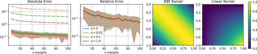
Figure 1: Absolute and relative error for the estimated Sinkhorn divergence between an RBF and linear kernel on $[0,1]$ as the amount of margins is increased. Solid lines represent the average for random sampling (shaded area illustrates $\sigma$-confidence intervals), and dot-dashed lines are upper bounds for the expected errors. The blue curve in the first plot is hidden behind the yellow one.

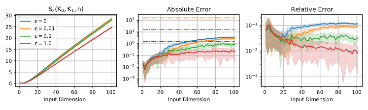
Figure 2: Absolute error and relative error for the estimated Sinkhorn divergence between an RBF and a linear kernel on $[0,1]^{d}$, where $d$ is the input dimension. The dot-dashed lines are the upper bounds for the expected errors.

4 Experiments

We now empirically illustrate the convergence by studying the behavior of the $2$-Sinkhorn divergence as we vary the entropic regularization $\epsilon$, amount $n$ of marginals used, and the input dimension of the kernels.

Varying amount of marginals.

We compute the divergence between the radial basis function (RBF) kernel with parameters $(\sigma^{2},\lambda)=(1,1)$ and linear kernel on $\mathcal{X}=[0,1]$ with a varying amount of marginals, sampled randomly from $\mathcal{X}$ ($m=50$ samples from the uniform distribution). The error is estimated by computing a ’ground truth’ using $n=1000$ uniformly sampled marginals.

The results in Fig. 1 illustrate that as we increase $\epsilon$, the absolute error

$$\left|S_{2,\epsilon}(K_{0},K_{1})-S_{2,\epsilon}(K_{0},K_{1},n)\right|$$ (56)

goes down as expected from Theorem 7. However, the relative errors

$$\frac{\left|S_{2,\epsilon}(K_{0},K_{1})-S_{2,\epsilon}(K_{0},K_{1},n)\right|}{S_{2,\epsilon}(K_{0},K_{1})}$$ (57)

stay almost identical. This is perhaps a bit disappointing, as one might hope $\epsilon$ to increase the relative accuracy too.

Varying input dimension.

In this experiment, we demonstrate the effect of the input dimension (dimensionality of $\mathcal{X}$) on the Sinkhorn divergence. We again consider the RBF kernel, with unit variances and length scales, and the linear kernel. For each dimension, we sample $n=100$ marginals $m=50$ times, and compare the resulting divergences to a ’ground truth’ computed with $n=1000$ samples.

As can be seen in Fig. 2, increasing the input dimension also increases the divergence between the kernels, seemingly in an unbouded manner. However, the absolute errors still remain bounded below the theoretical average error bounds, with increasing $\epsilon$ reducing the error. The interesting part is the behavior of the relative error as the dimension increases, as now we witness a reduction as we increase $\epsilon$, in contrast to the experiment with increasing marginals.

5 Conclusion

We have shown that the expected error of estimating the $2$-Sinkhorn divergence between GPs using $n$ marginals behaves as $\mathcal{O}\left(\epsilon^{-1}n^{-\frac{1}{2}}\right)$, implying that entropic regularization helps estimating the divergence. However, as $\epsilon$ increases, the Sinkhorn divergence converges to MMD, which is zero between covariance operators, and thus the divergence keeps decreasing. Therefore it is not surprising, that also the absolute errors should decrease.

Therefore the interesting quantity is the relative error of the estimate, which entropic regularization seems to help only as we increase the input dimension. This aligns well with what is known about OT and MMD: OT suffers from the curse of dimensionality, where as MMD benefits from dimension-free convergence rates. Notably, the error rates provided in the entropy-regularize case (Theorems 7 and 5) are dimension-free, and the demonstrations imply that the larger the regularization, the better the behavior with respect to input dimension.

References

- Arsigny et al. (2006) Arsigny, V., Fillard, P., Pennec, X., and Ayache, N. Log-Euclidean metrics for fast and simple calculus on diffusion tensors. Magnetic Resonance in Medicine: An Official Journal of the International Society for Magnetic Resonance in Medicine, 56(2):411–421, 2006.
- Bhatia (1997) Bhatia, R. Matrix Analysis. Springer, 1997.
- Chen & Zhu (2011) Chen, Y.-X. and Zhu, W.-J. Note on the strong law of large numbers in a Hilbert space. Gen. Math, 19(3):11–18, 2011.
- Cuturi (2013) Cuturi, M. Sinkhorn distances: Lightspeed computation of optimal transport. In Advances in neural information processing systems, pp. 2292–2300, 2013.
- del Barrio & Loubes (2020) del Barrio, E. and Loubes, J.-M. The statistical effect of entropic regularization in optimal transportation. arXiv preprint arXiv:2006.05199, 2020.
- Dessein et al. (2018) Dessein, A., Papadakis, N., and Rouas, J.-L. Regularized optimal transport and the rot mover’s distance. The Journal of Machine Learning Research, 19(1):590–642, 2018.
- Di Marino & Gerolin (2020) Di Marino, S. and Gerolin, A. Optimal transport losses and Sinkhorn algorithm with general convex regularization. arXiv preprint arXiv:2007.00976, 2020.
- Dowson & Landau (1982) Dowson, D. and Landau, B. The Fréchet distance between multivariate normal distributions. Journal of multivariate analysis, 12(3):450–455, 1982.
- Dudley (1969) Dudley, R. M. The speed of mean Glivenko-Cantelli convergence. The Annals of Mathematical Statistics, 40(1):40–50, 1969.
- Faraki et al. (2015) Faraki, M., Harandi, M. T., and Porikli, F. Approximate infinite-dimensional region covariance descriptors for image classification. In 2015 IEEE international conference on acoustics, speech and signal processing (ICASSP), pp. 1364–1368. IEEE, 2015.
- Feydy et al. (2019) Feydy, J., Séjourné, T., Vialard, F.-X., Amari, S.-i., Trouvé, A., and Peyré, G. Interpolating between optimal transport and MMD using Sinkhorn divergences. In The 22nd International Conference on Artificial Intelligence and Statistics, pp. 2681–2690. PMLR, 2019.
- Gelbrich (1990) Gelbrich, M. On a formula for the L2 Wasserstein metric between measures on Euclidean and Hilbert spaces. Mathematische Nachrichten, 147(1):185–203, 1990.
- Genevay et al. (2018) Genevay, A., Peyre, G., and Cuturi, M. Learning generative models with Sinkhorn divergences. In Storkey, A. and Perez-Cruz, F. (eds.), Proceedings of the Twenty-First International Conference on Artificial Intelligence and Statistics, volume 84 of Proceedings of Machine Learning Research, pp. 1608–1617, 2018.
- Genevay et al. (2019) Genevay, A., Chizat, L., Bach, F., Cuturi, M., and Peyré, G. Sample complexity of Sinkhorn divergences. In Chaudhuri, K. and Sugiyama, M. (eds.), Proceedings of Machine Learning Research, volume 89 of Proceedings of Machine Learning Research, pp. 1574–1583, 2019.
- Gerolin et al. (2019) Gerolin, A., Grossi, J., and Gori-Giorgi, P. Kinetic correlation functionals from the entropic regularisation of the strictly-correlated electrons problem. arXiv:1911.05818, 2019.
- Givens et al. (1984) Givens, C. R., Shortt, R. M., et al. A class of Wasserstein metrics for probability distributions. The Michigan Mathematical Journal, 31(2):231–240, 1984.
- Harandi et al. (2014) Harandi, M., Salzmann, M., and Porikli, F. Bregman divergences for infinite dimensional covariance matrices. In Proceedings of the IEEE Conference on Computer Vision and Pattern Recognition, pp. 1003–1010, 2014.
- Hauberg et al. (2015) Hauberg, S., Schober, M., Liptrot, M., Hennig, P., and Feragen, A. A random Riemannian metric for probabilistic shortest-path tractography. In International Conference on Medical Image Computing and Computer-Assisted Intervention, pp. 597–604. Springer, 2015.
- Janati et al. (2020) Janati, H., Muzellec, B., Peyré, G., and Cuturi, M. Entropic optimal transport between (unbalanced) Gaussian measures has a closed form. arXiv preprint arXiv:2006.02572, 2020.
- Kato (1987) Kato, T. Variation of discrete spectra. Communications in Mathematical Physics, 111(3):501–504, 1987.
- Knott & Smith (1984) Knott, M. and Smith, C. S. On the optimal mapping of distributions. Journal of Optimization Theory and Applications, 43(1):39–49, 1984.
- Lê et al. (2015) Lê, M., Unkelbach, J., Ayache, N., and Delingette, H. Gpssi: Gaussian process for sampling segmentations of images. In International Conference on Medical Image Computing and Computer-Assisted Intervention, pp. 38–46. Springer, 2015.
- Mallasto & Feragen (2017) Mallasto, A. and Feragen, A. Learning from uncertain curves: The 2-Wasserstein metric for Gaussian processes. In Advances in Neural Information Processing Systems, pp. 5660–5670, 2017.
- Mallasto et al. (2020) Mallasto, A., Gerolin, A., and Minh, H. Entropy-regularized 2-Wasserstein distance between Gaussian measures. preprint arXiv:2006.03416, 2020.
- Masarotto et al. (2019) Masarotto, V., Panaretos, V. M., and Zemel, Y. Procrustes metrics on covariance operators and optimal transportation of gaussian processes. Sankhya A, 81(1):172–213, 2019.
- Mena & Weed (2019) Mena, G. and Weed, J. Statistical bounds for entropic optimal transport: sample complexity and the central limit theorem. arXiv preprint arXiv:1905.11882, 2019.
- Minh (2015) Minh, H. Q. Affine-invariant Riemannian distance between infinite-dimensional covariance operators. In International Conference on Geometric Science of Information, pp. 30–38. Springer, 2015.
- Minh (2020) Minh, H. Q. Entropic regularization of Wasserstein distance between infinite-dimensional Gaussian measures and Gaussian processes. arXiv preprint arXiv:2011.07489, 2020.
- Minh et al. (2014) Minh, H. Q., San Biagio, M., and Murino, V. Log-Hilbert-Schmidt metric between positive definite operators on Hilbert spaces. In Advances in neural information processing systems, pp. 388–396, 2014.
- Olkin & Pukelsheim (1982) Olkin, I. and Pukelsheim, F. The distance between two random vectors with given dispersion matrices. Linear Algebra and its Applications, 48:257–263, 1982.
- Pennec et al. (2006) Pennec, X., Fillard, P., and Ayache, N. A Riemannian framework for tensor computing. International Journal of computer vision, 66(1):41–66, 2006.
- Peyré et al. (2019) Peyré, G., Cuturi, M., et al. Computational optimal transport: With applications to data science. Foundations and Trends® in Machine Learning, 11(5-6):355–607, 2019.
- Pigoli et al. (2014) Pigoli, D., Aston, J. A., Dryden, I. L., and Secchi, P. Distances and inference for covariance operators. Biometrika, 101(2):409–422, 2014.
- Pinelis (1994) Pinelis, I. Optimum bounds for the distributions of martingales in Banach spaces. The Annals of Probability, pp. 1679–1706, 1994.
- Ripani (2017) Ripani, L. The Schrödinger problem and its links to optimal transport and functional inequalities. Ph.D. thesis, University Lyon 1, 2017.
- Roberts et al. (2013) Roberts, S., Osborne, M., Ebden, M., Reece, S., Gibson, N., and Aigrain, S. Gaussian processes for time-series modelling. Philosophical Transactions of the Royal Society A: Mathematical, Physical and Engineering Sciences, 371(1984):20110550, 2013.
- Rosasco et al. (2010) Rosasco, L., Belkin, M., and De Vito, E. On learning with integral operators. Journal of Machine Learning Research, 11(30):905–934, 2010.
- Simon (2005) Simon, B. Trace ideals and their applications. Number 120. American Mathematical Soc., 2005.
- Villani (2008) Villani, C. Optimal transport: old and new, volume 338. Springer Science & Business Media, 2008.
- Weinzierl (2000) Weinzierl, S. Introduction to Monte Carlo methods. arXiv preprint hep-ph/0006269, 2000.