Spatial Functional Data Modeling of Plant Reflectances

Abstract

Plant reflectance spectra – the profile of light reflected by leaves across different wavelengths - supply the spectral signature for a species at a spatial location to enable estimation of functional and taxonomic diversity for plants. We consider leaf spectra as “responses” to be explained spatially. These spectra/reflectances are functions over a wavelength band that respond to the environment.

Our motivating data are gathered for several families from the Cape Floristic Region (CFR) in South Africa and lead us to develop rich novel spatial models that can explain spectra for genera within families. Wavelength responses for an individual leaf are viewed as a function of wavelength, leading to functional data modeling. Local environmental features become covariates. We introduce wavelength - covariate interaction since the response to environmental regressors may vary with wavelength, so may variance. Formal spatial modeling enables prediction of reflectances for genera at unobserved locations with known environmental features. We incorporate spatial dependence, wavelength dependence, and space-wavelength interaction (in the spirit of space-time interaction). We implement out-of-sample validation to select a best model, discovering that the model features listed above are all informative for the functional data analysis. We then supply interpretation of the results under the selected model.

arXiv:0000.0000

, , , , and

t1Corresponding Author

1 Introduction

The reflectance of the surface of a material is the fraction of incident electromagnetic radiation reflected at the surface. It is a function of the wavelength (or frequency) of the light, its polarization, and the angle of incidence. The reflectance as a function of wavelength is called a reflectance spectrum. The literature on reflectances is substantial, with a large portion focused on the interaction of electromagnetic energy with the atmosphere and terrestrial objects, e.g., reflectances associated with different land cover/vegetation types. Typically, they are gathered by satellites, aircraft, and ground-level sensors. The focus of this manuscript is on plant reflectances, i.e., data gathered for plants at leaf level.

The importance of leaf level reflectance modeling arises because the scales at which remote sensing devices detect reflectance spectra often do not match those relevant to ecological scales (Gamon et al., 2020). For example, a satellite imager can measure the reflectance signal for an entire $30\textrm{m}^{2}$ pixel; the reflectance signal of this pixel would be a composite of all the different spectral signatures of the plant species within that area. To disentangle what plants are on the ground, remote sensing scientists use spectral unmixing techniques which rely on spectral libraries (Quintano et al., 2012; Shi and Wang, 2014). These libraries are collections of pure endmembers, i.e., the pure reflectance spectra of leaf surfaces, which serve as representative spectra for different plant functional types, plant taxonomic groups, and/or individual plant species. Use of such leaf spectral libraries in ecology or biodiversity science has been termed as a “spectranomic” approach (Asner and Martin, 2016). Being able to statistically predict leaf reflectance spectra across environmental gradients constitutes a major advancement because it enables prediction-based spectral libraries that could be used in the validation and inference of remote sensing data at large spatial extents. Large hyperspectral remote sensing efforts are already under way, e.g., NASA’s Surface Biology Geology satellite mission (Cawse-Nicholson, 2021), making pressing the need to predict spectral signals of plants.

Furthermore, leaf-level spectra have become an invaluable tool to capture the diversity in leaf traits that have accumulated over the course of seed plant evolution (Reich et al., 2003; Cornwell et al., 2014) enabling estimation of functional diversity (Kokaly et al., 2009; Schneider et al., 2017) and taxonomic diversity (Clark, Roberts and Clark, 2005; Cavender-Bares et al., 2016a). They provide drivers for ecosystem processes (Schweiger et al., 2018) and guide conservation (Asner et al., 2017).

Statistical analyses of plant reflectance spectra have been limited to treating spectra as functional predictors of scalar variables such as plant traits. That is, we are in the realm of functional linear regression modeling. Modeling approaches rely on dimension reduction, e.g., spline basis representation (Ordoñez et al., 2010), partial least squares regression (Doughty, 2017), partial least squares-discriminant analysis (Cavender-Bares et al., 2016b), or some form of machine learning (Féret, 2019).

Some approaches generate hypothetical leaf reflectance spectra from physical first principles, i.e., radiative transfer models (Jacquemoud and Baret, 1990; Jacquemoud and Ustin, 2019a). However, these are not functional response models driven by environment. That is, our contribution is to model plant reflectance curves (as a function of wavelength) as a functional response variable, in particular, at genus level within family. We incorporate local spatial environmental covariates as regressors.

We introduce the following innovations, motivated by careful exploratory data analysis. We specify a functional data model incorporating spatial random effects to predict reflectance curves at genera level, at locations without collected plant samples. We also capture wavelength dependence through random effects. For further enrichment, we add space-wavelength interaction (in the spirit of space-time interaction) by constructing a space-wavelength random effect through wavelength kernel convolutions of spatial Gaussian processes. In general, this random effect has nonseparable covariance and is wavelength nonstationary. Additionally, we model the variance to be heterogeneous across wavelengths. Also, expecting that the reflectance response to environmental regressors may vary with wavelength, we include wavelength - covariate interactions. Lastly, because the rich space-wavelength modeling essentially annihilates the significance of the covariate/wavelength effects, we present a novel orthogonalization to remove spatial and functional confounding between random effects and environmental regressors.

Functional data analysis (FDA) is well established for analyzing data representing curves/surfaces varying over a continuum. The physical continuum over which these functions are defined is often time but here, it is wavelength. Pioneering work for FDA is attributed to Ramsey and Silverman (e.g., Ramsay, 2005; Ramsay and Silverman, 2007). The field has undergone rapid growth, and numerous applications have been found in areas such as imaging (Locantore et al., 1999) (including MRI brain imaging (Tian et al., 2010)), finance (Laukaitis, 2008), climatic variation (Besse, Cardot and Stephenson, 2000), spectrometry data (Reiss and Ogden, 2007), and time-course gene expression data (Leng and Müller, 2006). For a more comprehensive overview of applications, see Ullah and Finch (2013).

Explicit modeling of functional data is usually carried out by specifying functions in one of two ways: (i) as finite linear combinations of some set of basis functions or (ii) as realizations of some stochastic process. A key feature of functional data analysis implementation is some version of dimension reduction to specify functions. Here, we have random functions over a wavelength span as well as over a spatial region. We combine both approaches, using basis functions over wavelength with process realizations over space to build space by wavelength regressions over environment.

We work with plant reflectances gathered from the Cape Floristic Region (CFR) in South Africa. We present an extensive cross-validation study for model selection across a rich collection of models to demonstrate the ability of our space-wavelength modeling to predict reflectances well for genera within a family at unobserved locations. We present and discuss our findings for three plant families found within the CFR.

The format of the paper is as follows. Section 2 describes the collected data. Section 3 undertakes a broad exploratory data analysis to motivate the features we incorporate in our modeling. Section 4 explains our modeling, model comparison, and presents a novel orthogonalization for functional regression coefficients. Section 5 presents the analysis of the CFR data while a brief Section 6 offers a summary and suggestion for future work. Substantial detail of our exploratory analysis, as well as model sensitivity analysis, has been placed in the Supplemental Material.

2 The Dataset

We work with plant reflectances gathered from the Cape Floristic Region (CFR) in South Africa, see Figure 1. Reflectances were measured with a USB-4000 Spectrometer (manufactured by Ocean Optics) using a leaf clip attachment. Sun leaves from the top of each selected canopy were measured. The spectrometer has a range of 450-950 nanometers (nm) with a total of 500 reflectance measurements. We study plant reflectance viewed as a function of wavelength $t$, across the window $t\in[450,950)$, typically referred to as a spectral signature.

With interest in a spatial model for plant reflectance that enables prediction of reflectance for genera within a family at unobserved locations, we work with adjacent subregions of the CFR characterized by a fynbos landscape, known as the Hantam-Tanqua-Rogeveld (HTR) and Cederberg. Three prevalent families that often characterize landscapes in this area are Aizoaceae, Asteraceae, and Restionaceae (Slingsby and Wistow, 2014). These families have broad overlap in their reflectances (Figure 2). However, a linear discriminant analysis (LDA) to predict these families based on their reflectances yields clear separation of the groups, demonstrating that reflectances can be used to effectively predict taxonomic differences. More precisely, a structured classification by family using plant samples was conducted employing LDA and reveals the separation between families (See Supplemental Material for full details).

Much of the observed variation across the three families is likely due to differences in composite leaf traits though isolating the relative impact of each trait on the reflectances is beyond our intentions here. However, it is established that reflectance variation is a signal of leaf trait variation (e.g., anatomical, physiological, and structural traits (Jacquemoud and Ustin, 2019b)) and can be influenced by the environmental factors (e.g., climate and soil) that the plants inhabit.

3 Exploratory Data Analysis and Modeling

We explore the characteristics of plant reflectances for the three families given above (Aizoaceae, Asteraceae, Restionaceae) in the HTR and Cederberg areas. We retain the entire dataset because it is somewhat small from a spatial perspective. Note that the domains for the three families do not overlap well (Figure 1) so we will fit each family separately when implementing our spatial modeling.

The number of genera with observed reflectances within each family is: Aizoaceae - 16, Asteraceae - 38, and Restionaceae - 10. The Supplemental Material provides: (i) the proportion of sites where each family is present, (ii) the number of sites with one, two, or three families, and (iii) a more detailed breakdown of family co-occurrence. To summarize, Aizoaceae and Restionaceae rarely co-occur; in fact, Restionaceae is mostly limited to the Cederberg region apart from a few HTR observations. Replication at the genus level is uncommon and even more uncommon at the species level.

3.1 Data Locations

In Figure 1, we show all locations, where reflectances are observed with sites coded by region (shape) and family (color). We also plot locations coded by the number of families observed at that site. In the HTR and Cederberg regions, only 22 of the 133 sites have more than one reflectance spectrum for a given species; only 27 of the 183 total species (across all families) are observed at more than one site. This suggests that species-level modeling is infeasible. The Supplemental Material offers more commentary on data locations and duplication.

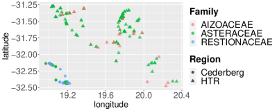
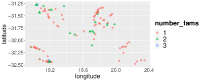
Figure 1: Locations (Left) colored by family with region-specific shapes and (Right) colored by the number of families observed at the site.

3.2 Reflectance spectra and Environmental Variables

To visualize the form and variability in reflectance spectra, we plot all of the curves by family in Figure 2 along with plots of the genus-specific means. We can see that the family-specific means do not capture the spread of the variability seen in all the curves while the genus-specific means show nearly the same variability for all of the curves.

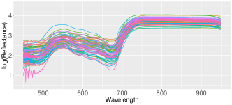
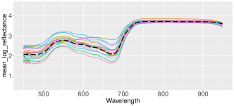
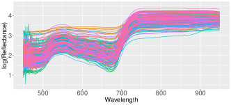
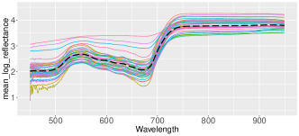
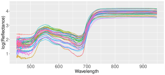
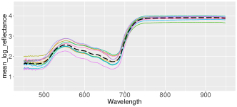
Figure 2: Log reflectances for Aizoaceae (Top-Left) All Curves, (Top-Right) Genus-specific means; Asteraceae (Middle-Left) All Curves, (Middle-Right) Genus-specific means; Restionaceae (Bottom-Left) All Curves, (Bottom-Right) Genus-specific means.

To assess within reflectance function variability as well as between-function variability, we calculate binned standard deviations for every curve. For these binned standard deviations, we estimate a smooth family-specific average standard deviation. Additionally, we calculate the family-specific between-curve standard deviation. These are plotted in Figure 3 and show that variability within reflectance spectrum changes with wavelength and, perhaps, with family. In addition, the variability between curves changes as a function of wavelength and differs by family. These findings lead us to impose heterogeneity in variance across wavelength, adopting wavelength varying variance curve models on the log scale.

Given these plots, we are led to four modeling needs: (i) to allow for family and genus differences, (ii) to model heterogeneity for the reflectance spectrum because within-curve variability changes across wavelength (iii) to capture between-curve variability through spatial modeling and/or environmental variables, and (iv) to adopt heteroscedastic errors since reflectances at lower wavelengths ($<500$ nm) appear to be more volatile.

For each family, we calculate the correlations between the environmental variables (see Supplemental Material) and the observed log-reflectances, using wavelength bins (See Figure 4), to assess whether this relationship changes with wavelength. We find consequential changes in correlation as a function of wavelength. The strongest correlations are of magnitude 0.3 to 0.4.

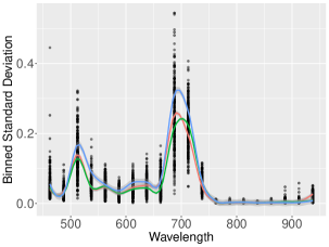
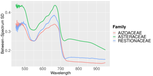
Figure 3: (Left) 25-nm binned standard deviations for each reflectance spectrum with smoothed family-specific curves. (Right) Family-specific between-spectrum standard deviation as a function of wavelength.

3.3 Environmental Variables and Reflectance Spectra

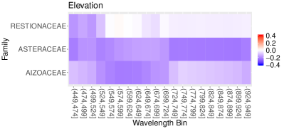
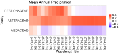
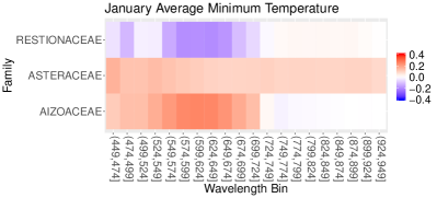
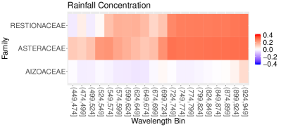
Figure 4: (Top-Left to Bottom-Right) elevation, mean annual precipitation, average minimum temperature in January, rainfall concentration.

4 Spatial Wavelength Modeling

Functional data modeling for our spatial reflectance spectra was motivated by the foregoing exploratory analyses. Families are modeled separately, at genus level, treating species within genus as replicates. We utilize the following environmental predictors: elevation, annual precipitation, rainfall concentration, and minimum January temperature. We introduce wavelength dependent variances to account for evident heterogeneity. Model choice focuses on four issues: (i) Do we need wavelength dependent regression coefficients? (ii) Do we need genus specific wavelength random effects? (iii) Do we need genus specific spatial random effects? (iv) How do we specify space-wavelength interaction?

In Sections 4.1 and 4.2, we elaborate the models, while Section 4.3 takes up model comparison yielding the model for which results are presented.

4.1 Model development

For a given family, let $i$ denote genera within the particular family, let $j$ denote replicates/species within genus. Let s denote spatial location and $t$ denote wavelength. There is severe imbalance in the data. The genera observed vary across locations and the number of replicates observed within a genus varies considerably across the locations. Altogether, our most general model for log reflectance takes the form:

$$Y_{ij}(\textbf{s},t)=\mu_{i}(\textbf{s},t)+\gamma_{i}(t)+\alpha_{i}(\textbf{s})+\eta(\textbf{s},t)+\epsilon_{ij}(\textbf{s},t)$$ (1)

Specifically, with regard to the site level covariates, $\textbf{X}(\textbf{s})$, we write the mean $\mu_{i}(\textbf{s},t)=\alpha_{i}+\textbf{X}^{T}(\textbf{s})\mbox{\boldmath$\beta$}(t)$, where, hierarchically, $\alpha_{i}|\alpha\sim\mathcal{N}(\alpha,\sigma^{2}_{\alpha})$. We have family level regression coefficients, $\mbox{\boldmath$\beta$}(t)$, which vary with wavelength. So, a first model choice clarification is whether constant coefficients are adequate or whether wavelength varying coefficients are needed. Our EDA (Figure 4) suggests the latter, and there is also supporting evidence/suggestion in the literature (Jacquemoud and Ustin, 2019c). We do not consider these coefficients at genus level; with the very irregular observation (including absence) of genera across locations, we cannot learn about coefficients at genus scale. However, we can learn about genus specific intercepts, the $\alpha_{i}$.

Further, we introduce genus level spatial ($\alpha_{i}(\textbf{s})$) and wavelength ($\gamma_{i}(t)$) random effects but family level space-wavelength interaction effects, $\eta(\textbf{s},t)$. In the Supplemental Material, we note different spatial patterns for different wavelength bins, as well as residual dependence by genus and wavelength. Thus, an additive model (removing $\eta(\textbf{s},t)$) seems inadequate; the $\eta$’s allow the functional model for the reflectances to vary more adaptively over space. However, $\eta(\textbf{s},t)$ is not genus specific. While we have enough data to examine additivity in wavelength and spatial random effects at genus scale, we are unable to find genus level explanation for the interaction. Then, two model choice comparisons are whether the $\gamma$’s and whether the $\alpha$’s should still be genus specific?

As is customary, heterogeneity in the variance arises through the $\epsilon_{ij}(\textbf{s},t)$ terms where we would have $\text{var}(\epsilon_{ij}(\textbf{s},t))=\sigma^{2}(t)$. We can accommodate this using a log GP for $\sigma^{2}(t)$, or perhaps just binned variances over suitable wavelength bins. For simplicity and flexibility, we specify $\log(\sigma^{2}(t))$ to be piecewise linear with knots every 20 nm from 440 - 960 nm. For all knot selections, we use boundary knots slightly beyond the wavelength range.

4.2 Explicit Specifications

The specification for each $\alpha_{i}(\textbf{s})$ is a genus-level mean $0$ Gaussian process with mean of $0$ and exponential covariance function. The GPs are conditionally independent across genera given a shared decay and shared scale parameter. We specify $\gamma_{i}(t)$ using process convolution of normal random variables (Higdon, 1998, 2002). We adopt process convolutions because of their simple connection to GPs; the kernels of the process convolution connect the low-rank process to the GP covariance (Higdon, 1998). We adopt wavelength knots $t^{\gamma}_{1},...,t^{\gamma}_{J_{\gamma}}$, spaced every 25 nm from 437.5-962.5 nm (22 in total).

Specifically, we let $\gamma_{i}(t)=\sum^{J_{\gamma}}_{j=1}k_{t^{\gamma}_{j}}(t-t^{\gamma}_{j};\theta^{(\gamma)}_{t^{\gamma}_{j}})\gamma_{i}^{*}(t^{\gamma}_{j})$, where $\gamma_{i}^{*}(t^{\gamma}_{j})$ are independent, normally distributed, and centered on a common $\gamma^{*}(t^{\gamma}_{j})$. We use Gaussian kernels for $k_{t_{j}}(\cdot;\theta_{t_{j}}^{(\gamma)})$ with bandwidths $\theta_{t_{j}}^{(\gamma)}$ (standard deviation of the Gaussian pdf) varying over wavelength. We assume that the log-bandwidths follow a multivariate normal distribution with global log-bandwidth and
Cov$\left[\log\left(\theta_{t_{j}}^{(\gamma)}\right),\log\left(\theta_{t_{j^{\prime}}}^{(\gamma)}\right)\right]=v_{\gamma}^{2}\exp\left(-|t_{j}-t_{j^{\prime}}|/\phi_{\gamma}\right)$, yielding a non-stationary process because of the heterogeneous bandwidth. We found that this nonstationary specification outperformed a full-rank stationary GP with squared-exponential covariance (See Supplemental Material).

We specify $\mbox{\boldmath$\beta$}(t)$ using kernel convolutions, where $\mbox{\boldmath$\beta$}(t)=BK_{\beta}(t)$. With $p$ covariates, $B$ supplies a $p\times q$ matrix representation of the $p$ regression coefficient functions $\mbox{\boldmath$\beta$}(t)$. Here, the kernel convolution has knots every 25 nm from 437.5 - 962.5 nm. As with $\gamma_{i}(t)$, we use Gaussian kernels to specify $K_{\beta}(t)$; however, unlike $\gamma_{i}(t)$, we assume common bandwidths for all kernels, for all wavelengths, and for each coefficient function.

Turning to $\eta(\textbf{s},t)$, we use wavelength kernel convolutions of spatially-varying variables. That is, we consider low-rank but heterogeneous and nonstationary (in the wavelength domain) specifications. We select a set of wavelength knots $t^{\eta}_{1},...,t^{\eta}_{J_{\eta}}$, spaced every 25 nm from 437.5-962.5 nm (22, in total). We define the space-wavelength function as

$$\eta(\textbf{s},t)=\textbf{K}(t)^{T}\textbf{z}(\textbf{s})=\sum_{j=1}^{J_{\eta}}k_{t^{\eta}_{j}}(t-t^{\eta}_{j};\theta^{(\eta)})z_{t^{\eta}_{j}}(\textbf{s}),$$ (2)

where $z_{t^{\eta}_{j}}(\textbf{s})$ are spatially-varying random variables associated with Gaussian wavelength kernels $k_{t^{\eta}_{j}}(\cdot;\theta_{t^{\eta}_{j}})$. Unlike the kernel structure for $\gamma(t)$, we use a common bandwidth $\theta^{(\eta)}$ for all knots. The construction in (2) allows heterogeneity and nonstationarity in wavelength space, where the heterogeneity is introduced through $z_{t^{\eta}_{j}}(\textbf{s})$ (See White, Keeler and Rupper, 2021, for a similar construction in the context of spatial monotone regression).

As an aside, we remark on choosing the form $\eta(\textbf{s},t)=\textbf{K}^{T}(t)\textbf{z}(\textbf{s})$ vs. $\eta(\textbf{s},t)=\textbf{K}^{T}(\textbf{s})\textbf{z}(t)$. With $n$ sites, the former introduces $J_{\eta}n$ random effects, the latter $500n$ random effects. With $J_{\eta}$ relatively small, the former is preferred computationally. More importantly, it yields much better fits to the data (see the Supplemental Material).

While we may want dependence between components in $\textbf{z}(\textbf{s})$ at s, that dependence should have nothing to do with the $t^{\eta}_{j}$’s. We are capturing association with regard to the distances between wavelength knots through the $K$’s and our objective for the $z$’s is to obtain perhaps nonseparable and nonstationary covariance structure for $\eta(\textbf{s},t)$. So, we write $\textbf{z}(\textbf{s})=A\textbf{w}(\textbf{s})$ where $A$ is $J_{\eta}\times r$ and the components of $\textbf{w}(\textbf{s})$ are independent mean $0$ GP’s with variance $1$ and correlation functions, $\rho_{r}(\textbf{s}-\textbf{s}^{\prime})$.

When $r=J_{\eta}$, we have the familiar linear model of coregionalization (Wackernagel, 1998). We consider using $A=I$ and $A_{p\times r}$, for various $r$, as well as a separable specification for $\textbf{z}(\textbf{s})$, where, with V a positive definite matrix, $\text{Cov}\left(\textbf{z}(\textbf{s}),\textbf{z}(\textbf{s}^{\prime})\right)=\exp\left(-\phi_{z}\|\textbf{s}-\textbf{s}^{\prime}\|\right)\textbf{V}$. With $A_{p\times r}$, we constrain the decay parameters of the $(w_{1}(\textbf{s}),...,w_{r}(\textbf{s}))^{T}$ to be increasing (see White and Gelfand, 2020), so that the latent GPs have different spatial decays ($\phi_{z}$). The resulting processes for $\textbf{z}(\textbf{s})$ are very flexible. We compare the various choices through out-of-sample prediction in Section 4.3.

Under the general form $\eta(\textbf{s},t)=\textbf{K}^{T}(t)(\textbf{s})A\textbf{w}(\textbf{s})$, $\text{cov}(\eta(\textbf{s},t),\eta(\textbf{s}^{\prime},t^{\prime}))=\textbf{K}^{T}(t)A\Sigma_{\textbf{w}(\textbf{s}),\textbf{w}(\textbf{s}^{\prime})}A^{T}\textbf{K}(t^{\prime}).$ If $A=I$, we have $\Sigma_{\textbf{w}(\textbf{s}),\textbf{w}(\textbf{s}^{\prime})}=D(\textbf{s}-\textbf{s}^{\prime})$, a $J_{\eta}\times J_{\eta}$ diagonal matrix with entry $d_{jj}=\rho_{j}(\textbf{s}-\textbf{s}^{\prime})$. Thus, $\text{cov}(\eta(\textbf{s},t),\eta(\textbf{s}^{\prime},t^{\prime}))=\textbf{K}^{T}(t)D(\textbf{s}-\textbf{s}^{\prime})\textbf{K}(t^{\prime})=\sum_{j}k_{t^{\eta}_{j}}(t-t_{j})k_{t^{\eta}_{j}}(t^{\prime}-t^{\eta}_{j})\rho_{j}(\textbf{s}-\textbf{s}^{\prime})$. The covariance is always nonseparable and, if $A$ is unconstrained it is nonstationary.

As an illustration, if we take $A$ to be $J_{\eta}\times 2$, we have $\Sigma_{\textbf{w}(\textbf{s}),\textbf{w}(\textbf{s}^{\prime})}=\left(\begin{array}[]{cc}\rho_{1}(\textbf{s}-\textbf{s}^{\prime})&0\\ 0&\rho_{2}(\textbf{s}-\textbf{s}^{\prime})\\ \end{array}\right)$. Now, with $\textbf{a}_{1}$ and $\textbf{a}_{2}$ the two columns of $A$, $\text{cov}(\eta(\textbf{s},t),\eta(\textbf{s}^{\prime},t^{\prime}))=(\textbf{K}^{T}(t)\textbf{a}_{1})(\textbf{K}^{T}(t^{\prime})\textbf{a}_{1})\rho_{1}(\textbf{s}-\textbf{s}^{\prime})+(\textbf{K}^{T}(t)\textbf{a}_{2})(\textbf{K}^{T}(t^{\prime})\textbf{a}_{2})\\ \rho_{2}(\textbf{s}-\textbf{s}^{\prime})$. We achieve both dimension reduction and space-wavelength interaction. Further, we have nonseparability and nonstationarity (in the wavelengths) if there are different bandwidths for the different $t_{j}$. If we set $r=1$, we have separability but still nonstationarity in the wavelengths.

4.3 Model Comparison

We carry out model comparison for Asteraceae, the most abundant family, using 10-fold cross-validation (described below). In the Supplemental Material, we present cross-validation results examining various specifications of the spatial process in $\eta(\textbf{s},t)$. When comparing models with different specifications of $\eta(\textbf{s},t)$, all models include spatially-varying genus-specific intercepts $\alpha_{i}+\alpha_{i}(\textbf{s})$, a global (not genus-specific) wavelength random effect $\gamma(t)$, and functional regression coefficients $\mbox{\boldmath$\beta$}(t)$. For $\eta(\textbf{s},t)$, we compare separable, independent, and latent factor models. We find that the latent factor specification of $\eta(\textbf{s},t)$ with $r=10$ has the best out-of-sample predictive performance and use this for $\eta(\textbf{s},t)$ in the remainder of the manuscript. For this specification of $\eta(\textbf{s},t)$, we focus our model comparison on eight special cases of (1) arising by (i) including or excluding $\alpha_{i}(\textbf{s})$, (ii) using $\gamma_{i}(t)$ or only $\gamma(t)$, and (iii) having functional coefficients $\mbox{\boldmath$\beta$}(t)$ or scalar coefficients $\beta$.

We hold out reflectances imagining the setting where researchers visited a site but failed to measure reflectances for some genus at that site. So, at random, we leave out spectra that have (i) at least one other observed reflectance spectrum at the same site and (ii) at least one other observed spectrum of the same genus located elsewhere. For Asteraceae, this yields 117 candidates out of the 185 in total. Holding out a subset, we fit the model using Markov chain Monte Carlo, and, with each posterior sample, we predict the hold-out reflectance spectra. We compare models by averaging across the wavelengths to obtain the predicted mean squared error (MSE), mean absolute error (MAE), and the mean continuous ranked probability score (MRCPS), see Gneiting and Raftery (2007). The results are summarized in Tables 1 and in the Supplement.

$\alpha_{i}$/$\alpha_{i}(\textbf{s})$	$\gamma(t)$/$\gamma_{i}(t)$	$\beta$/$\mbox{\boldmath$\beta$}(t)$	MSE	MAE	MCRPS	Relative MCRPS
$\alpha_{i}$	$\gamma(t)$	$\beta$	0.148	0.301	0.241	1.229
$\alpha_{i}$	$\gamma(t)$	$\mbox{\boldmath$\beta$}(t)$	0.141	0.293	0.234	1.196
$\alpha_{i}$	$\gamma_{i}(t)$	$\beta$	0.175	0.320	0.265	1.355
$\alpha_{i}$	$\gamma_{i}(t)$	$\mbox{\boldmath$\beta$}(t)$	0.169	0.318	0.262	1.340
$\alpha_{i}(\textbf{s})$	$\gamma(t)$	$\beta$	0.102	0.244	0.200	1.023
$\alpha_{i}(\textbf{s})$	$\gamma(t)$	$\mbox{\boldmath$\beta$}(t)$	0.097	0.237	0.196	1.000
$\alpha_{i}(\textbf{s})$	$\gamma_{i}(t)$	$\beta$	0.348	0.435	0.393	2.009
$\alpha_{i}(\textbf{s})$	$\gamma_{i}(t)$	$\mbox{\boldmath$\beta$}(t)$	0.290	0.420	0.380	1.940

Table 1: Out-of-sample predictive performance model comparison. Models vary by including or excluding genus-specific terms, as well as comparing scalar and functional coefficients. All models use $r=10$ spatial factors to construct $\eta(\textbf{s},t)$.

Following the results in Table 1 and the Supplemental Material, we adopt a model with (1) a global wavelength random effect, (2) a spatially-varying genus-specific intercept, (3) functional regression coefficients, and (4) a space-wavelength random effect specified through the wavelength kernel convolution of a multivariate spatial process with 10 latent spatial GPs having different decay parameters. We use this model to analyze the CFR data.

For the sensitivity of model fit to change in other specifications (e.g., knot spacing and GP/process convolution), we use average deviance, the deviance information criterion, and estimated model complexity (Spiegelhalter et al., 2002), as supplied in the Supplemental Material. To summarize, we employ a heterogeneous process convolution specification of $\gamma(t)$ because it gave a better fit than a full-rank homogeneous GP with squared-exponential covariance and a process convolution with a common bandwidth for all wavelength knots. We also specify $\mbox{\boldmath$\beta$}(t)$ using kernel convolutions where $\mbox{\boldmath$\beta$}(t)=BK_{\beta}(t)$, where we space knots every 25 nm from 437.5 - 962.5 nm. We also find that the Gaussian kernel, which corresponds to the Gaussian covariance function, was preferred to using double-exponential kernels for $\gamma(t)$, $\mbox{\boldmath$\beta$}(t)$, and $\eta(\textbf{s},t)$. For $\gamma(t)$, the model fit was improved when bandwidths $\theta^{(\gamma)}_{t_{j}}$ varied over wavelength; however, a common bandwidth for the kernels was prefered for $\eta(\textbf{s},t)$. The knot spacing, discussed in Section 4.2, was also determined through sensitivity analysis.

4.4 Confounding and Orthogonalization

The flexibility of the residual specification in our best performing model results in annihilation of the significance of the spatial regressors. This is a well-documented problem in the literature (see, e.g., Hodges and Reich, 2010; Khan and Calder, 2020). A solution in the literature is orthogonalization; that is, projection of the random effects (the spatial residuals) onto the orthogonal complement of the manifold spanned by the spatial covariates. This yields revised regression coefficients with direct interpretation in the presence of the random effects. The coefficients are more aligned with those that arise from model fitting ignoring spatial random effects.

We propose a similar orthogonalization approach here but our setting is more demanding because we have both space and wavelengths in our residuals. We have to introduce orthogonalization with regard to the manifold spanned by the spatial covariates as well as with regard to the manifold spanned through the use of kernel functions with knots. We present the details below for the simpler case where we have no replicates at locations. However, in our application, we have replicates associated with the spatial locations and also with different genera. So, formally, the orthogonalization requires us to introduce a location by genus matrix to align the number of observed sites with the number of observed reflectances. We present the more detailed argument in the Supplemental Material.

With $n$ sites and $500$ wavelengths, we can express (1) in matrix form as

$$Y=\alpha\textbf{1}+XBK_{\beta}^{T}+\eta^{*}+\epsilon$$ (3)

where $Y$ is the $n\times 500$ matrix of log-reflectance spectra data by sites, 1 is a $n\times 500$ matrix of ones, $\alpha$ is the global mean, $X$ is the $n\times p$ spatial design matrix (with $p$ covariates), $B$ is $p\times J_{\beta}$ with $J_{\beta}$ knots, $K_{\beta}$ is the $500\times J_{\beta}$ kernel design matrix with $J_{\beta}$ knots. $\eta^{*}$ is also $n\times 500$ summing the corresponding matrix forms for the mean-zero random effects ($\gamma(t)$, $\alpha_{i}(\textbf{s})$, $\alpha_{i}-\alpha$, and $\eta(\textbf{s},t)$). Then, using standard results, we can vectorize (3) to

$$vec(Y)=\alpha\textbf{1}+(X\otimes K_{\beta})vec(B)+vec(\eta*)+vec(\epsilon)$$ (4)

where $vec(Y)$ is an $n500\times 1$ vector with $X\otimes K_{\beta}$ an $n500\times pJ$ matrix.

Now, define the joint projection matrix,

$$P_{XK_{\beta}} \equiv(X\otimes K_{\beta})((X\otimes K_{\beta})^{T}(X\otimes K_{\beta}))^{-1}(X\otimes K_{\beta})^{T}$$ (5)

$$=(X(X^{T}X)^{-1}X^{T})\otimes(K_{\beta}(K_{\beta}^{T}K_{\beta})^{-1}K_{\beta}^{T})=P_{X}\otimes P_{K_{\beta}},$$

and write $vec(\eta^{*})=P_{XK_{\beta}}vec(\eta^{*})+(I-P_{XK_{\beta}})vec(\eta^{*})$. Then, we can write $vec(Y)=(X\otimes K_{\beta})vec(B^{*})+(I-P_{XK_{\beta}})vec(\eta^{*})+vec(\epsilon)$, where the updated unconfounded coefficients are (in vec and block form)

$$vec(B^{*}) =vec(B)+((X\otimes K_{\beta})^{T}(X\otimes K_{\beta}))^{-1}(X\otimes K_{\beta})^{T}vec(\eta^{*}),$$ (6)

$$B^{*} =B+(X^{T}X)^{-1}X^{T}\eta^{*}K_{\beta}(K_{\beta}^{T}K_{\beta})^{-1}.$$

Here, $vec(B^{*})$ and $B^{*}$ provide the vector and matrix of regression coefficients, respectively, under the orthogonalization. The model is fitted using (1). Then, with the posterior samples of the $\beta$’s, $\gamma$’s, $\alpha$’s, and $\eta$’s along with the $\textbf{X}(\textbf{s})$ and $\textbf{K}_{\beta}(t)$, the unconfounded $B^{*}$’s can be obtained using (6).

5 Analysis of the CFR Reflectance Spectra Data

We focus discussion on a comparison between families but give specific attention to the results on Asteraceae, the most abundant family. We compare and discuss results from the orthogonalized coefficients using the approach in Section 4.4. In addition, we summarize covariate importance on log-reflectance. Again using the orthogonalized random effects and unconfounded regression functions, we discuss the proportion of variance explained by each model term.

The confounding between random effects (genus, wavelength, and spatial) and covariates pushes $\mbox{\boldmath$\beta$}(t)$ to zero, obliterating any significant inference with regard to the effect of environmental variables on log-reflectance. For each MCMC posterior sample, we calculate the proportion of the variance in each random effect ($\alpha_{i}(\textbf{s})$, $\gamma(t)$, $\eta(\textbf{s},t)$) explained by X and $\textbf{K}_{\beta}$. We orthogonalize our random effects with respect to X and $\textbf{K}_{\beta}$ as described in Section 4.4 to remove the diminishing of the effect of the regressors.

For the Asteraceae family, we explore the proportion of the variance explained by each of the mean-zero model terms. For every posterior sample, we calculate the empirical variance of all nonorthogonalized and orthogonalized terms (See Figure 5 to the 95% credible regions): $\epsilon_{ij}(\textbf{s},t)$, $\textbf{x}(s)^{T}\mbox{\boldmath$\beta$}(t)$, $\alpha_{i}(\textbf{s})+\alpha_{i}-\alpha$, $\gamma(t)$, and $\eta(\textbf{s},t)$. We take $\alpha_{i}(\textbf{s})+\alpha_{i}$ to capture both genus-specific terms and subtract $\alpha$ to make $\alpha_{i}(\textbf{s})+\alpha_{i}-\alpha$ a mean-zero random effect. For orthogonalized terms, $\gamma(t)$ explains slightly under 25% of the variability of the data, while both $\eta(\textbf{s},t)$ and $\textbf{x}(s)^{T}\mbox{\boldmath$\beta$}(t)$ explain over 30% of the total variance. Without orthogonalization of the random effects, the environmental regression explains almost no variance. The genus-specific spatially-varying intercept $(\alpha_{i}(\textbf{s})+\alpha_{i})-\alpha$ explains over 10% of the total variance while $\epsilon_{ij}(\textbf{s},t)$ accounts for about 5% of variance in the data.

In Figure 5, we plot the proportion of between-spectrum variability explained by all orthogonalized mean-zero terms as a function of wavelength (posterior mean and 95% credible interval). Even though $\gamma(t)$ is common to all spectra, after orthogonalization, it is no longer a constant term for all spectra. For wavelengths less than 700 nm, we find that unconfounded environmental regression and space-wavelength random effects are most important in explaining between-spectrum variance. For higher wavelengths ($>750$ nm), where there is little variation in the wavelength functions; the orthogonalized global wavelength random effects $\gamma(t)$ and the unconfounded environmental regression explain the most between-spectrum variance. The spatially-varying genus-specific offset, $(\alpha_{i}(\textbf{s})+\alpha_{i})-\alpha$ explains between 10-20% of between-spectrum variance for most wavelengths but appears particularly influential for wavelengths between (675-725 nm). The $\epsilon_{ij}(\textbf{s},t)$ account for the 0 to 10% of unexplained between-spectrum variance in log-reflectance, depending on wavelength.

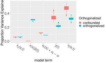
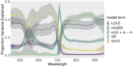
Figure 5: (Left) Proportion of variance explained by each model term and (Right) Proportion of between-site variance explained by model terms.

After updating $\mbox{\boldmath$\beta$}(t)$ in the presence of orthogonalization, we present inference on covariates for all families. Figure 6 shows the posterior mean, 95% credible interval for each element of $\mbox{\boldmath$\beta$}(t)$. All coefficient functions are significantly non-zero for most wavelengths (around 99% for all wavelengths). With covariates centered and scaled, (i) we can interpret effects as the expected change in log-reflectance for a one standard deviation change in the covariate, holding the other covariates constant, and (ii) we can compare the scales of the coefficient functions among covariates.

The four covariates have positive effects for some wavelengths, negative effects for others, with a transition around 700 nm, a threshold/boundary between visible (450-700nm) and near-infrared regions (NIR, 700-1400nm) of the spectrum. The visible region is most strongly affected by differences in plant pigment composition/concentration while the NIR is most affected by structural properties related to the cell wall, to air interface within the leaf (Jacquemoud and Ustin, 2019c). Traits can exhibit uniform effects across multiple parts of the spectrum (e.g., often in water content) or can cause increased reflectance in parts of the spectrum and decreased reflectance in others (Feng et al., 2008; Jacquemoud and Ustin, 2019b). Different sets of traits acting in concert in response to environment likely drive the positive and negative shifts across the 700 nm threshold in Figure 6.

For Asteraceae, we estimate that higher elevations are associated with lower reflectance levels at wavelengths less than 700 nm but higher reflectance at wavelengths above 700 nm. The relationships of precipitation and temperature with reflectance are similar. On the other hand, rainfall concentration is positively correlated with reflectance at low wavelengths and becomes negatively correlated with reflectance as wavelength increases. We note that rainfall concentration, the environmental feature that reflectance responds differently to, is largely longitudinally driven in comparison to the other features. Specifically, the extreme western and to some extent the extreme eastern sample sites have significantly higher rainfall concentrations than more central locations. Because there is between-covariate correlation, the coefficient functions must be interpreted as partial slopes, i.e., holding all other covariates constant.

To compare covariate importance, we calculate the mean integrated absolute coefficient over the wavelength domain, $\overline{|\beta_{j}|}=\frac{1}{500}\int_{450}^{950}|\beta_{j}(t)|dt\approx\frac{1}{500}\sum_{i=1}^{500}|\beta_{j}(t_{i})|,$ for each covariate. This metric weights the contribution of the coefficient equally regardless of sign or wavelength. We calculate $\overline{|\beta_{j}|}$ for every posterior sample and plot these in Figure 7. In terms of $\overline{|\beta_{j}|}$, elevation and temperature are more influential on reflectance than precipitation and rainfall concentration.

5.1 Comparison across families

We compare the regression coefficient functions for the three families in this study (posterior mean and 95% credible interval): Aizoaceae, Asteraceae, and Restionaceae (See Figure 6). The regression coefficient functions are clearly distinct across the families. However, between-covariate correlation or different spatial sites covered by each family may account for some of these differences.

The estimated effects of elevation, annual precipitation, and temperature are opposite in direction for all wavelengths between Asteraceae and Aizoaceae. For these covariates, we see positive effects on Aizoaceae log-Reflectance for wavelengths $<700$ nm and negative effects for wavelengths $>700$ nm, with opposite patterns for Asteraceae. For Asteraceae, the estimated effects of rainfall concentration are positive for lower wavelengths and negative for higher wavelengths, while they are nearly zero for Aizoaceae. Restionaceae has very small estimated temperature effects. For elevation and rainfall concentration, Restionaceae shows significant effects on log-reflectance for wavelengths $<700$ nm, but essentially no effect for higher wavelengths. The estimated effect of precipitation for Restionaceae is similar to Aizoaceae in pattern but is smaller in magnitude.

In Figure 6, we also plot the variance function for $\epsilon_{ij}(\textbf{s},t)$ for each family (posterior mean and 95% credible interval). Asteraceae has the highest estimated variance for most low wavelengths (450 - 700 nm), a trend that matches the between spectrum variance patterns in Figure 3. Restionaceae has the lowest estimated variance for (450 - 700 nm). All families have very low estimated variance for most high wavelengths (700 - 950 nm).

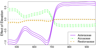
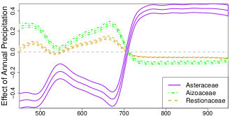
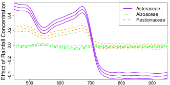
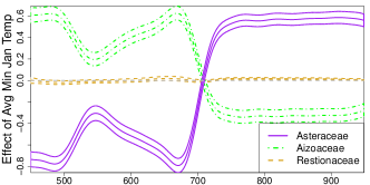
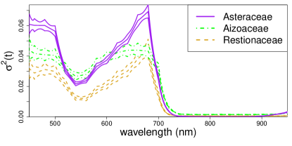
Figure 6: Between family comparison of (Top-Left to Middle-Right) environmental regression coefficient functions (Elevation, Annual Precipitation, Rainfall Concentration, and Average Minimum January Temperature) and (Bottom) wavelength-varying variance $\sigma^{2}(t)$.

The differing responses in visible and near-infrared reflectance to environment between Aizoaceae and Asteraceae 6 likely indicate that genera within the two families employ different adaptive strategies in response to their local environments across the landscape. The Aizoaceae family consists of small succulent stemmed and leafed plants while the Asteraceae family largely consists of non-succulent leafed herbs and shrubs. Both plant families adapt via other traits tied to aridity tolerance (e.g., water storage for periods of drought) and avoidance (e.g., leaf hairs, wax, and anthocyanin pigmentation that block UV radiation). The adaptive traits in the respective ”evolutionary toolboxes” of Aizoaceae and Asteraceae are constrained by their phylogenetic ancestry, resulting in differing strategic responses to environment in their traits and thus, reflectances. In contrast, the Restionaceae consist of grass-like plants with tough fibrous photosynthetic stems that vary less than the other two families in adaptation to drought.

We show the posterior distribution (box plots) for $\overline{|\beta_{j}|}$ across all covariates and families (See Figure 7). Since $\overline{|\beta_{j}|}$ represents the relative importance of covariates for log-reflectance, we see that the covariates are more important in describing log-reflectances for Asteraceae than Aizoaceae and more important for Aizoaceae than for Restionaceae, except for rainfall concentration. Perhaps the relative importance $\overline{|\beta_{j}|}$ may be higher for Aizoaceae and Asteraceae because these have more expansive spatial distributions and thus experience higher variability in environmental variables.

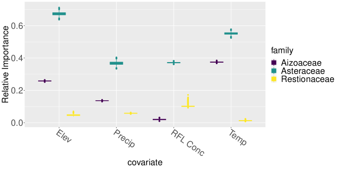
Figure 7: Covariate importance $\overline{|\beta|}$ for all families.

Despite the differences in spatial ranges, the families differ in terms of which environmental variables have the highest relative importance to their reflectance signals. The most important variable for Asteraceae is elevation, likely a proxy for several environmental factors; prominent among them is the biome shift from the higher elevation Fynbos biome within the Cederberg mountains to the lower elevated Succulent Karoo biome. These biomes differ widely in their environments, the Fynbos biome having nutrient-poor soils and a regular fire cycle while the Succulent Karoo is largely arid with low levels of rainfall. Asteraceae is the only family to fully span both biomes in large numbers and these biomes feature a wide difference in environments. The most important variable for Aizoaceae is the minimum average temperate in January (the peak austral summer month), a strong indicator of the maximum temperature a plant can tolerate. This suggests that the major driver of Aizoaceae reflectances are underlying adaptations related to heat tolerance/avoidance. While more limited in its spatial extent, the Restionaceae reflectance spectra responded most to rainfall concentration. Under the notion that higher concentrations of rainfall in fewer months out of the year would lead to more dramatic periods without water, much of the differences in Restionanceae reflectance may be in response to underlying traits managing water during times of drought.

6 Summary and Future Work

We have offered plant reflectance modeling to capture variation over space between reflectance across genera within a family. We incorporate wavelength heterogeneity, spatial dependence, and also wavelength - covariate interaction as well as space - wavelength interaction. We have fitted these models to reflectances from the Cape Floristic Region in South Africa, demonstrating successful model performance and revealing a range of novel inference as well as successful spatial prediction.

This work has several future applications and opportunities for further development. Our current data only included the visible and near-infrared reflectance spectra of leaves. These data could be expanded to include the reflectance of plant canopies across a broader spectral range to make predictions relevant to the reflectance spectra collected by broader band sensors aboard aerial and satellite remote sensing platforms. Our spatially explicit predictions of plant reflectance would be highly relevant for spectral unmixing analyses which seek to predict the abundances of spectral end members, i.e., individual species, in a canopy of vegetation. Future modeling efforts include exploring reflectance signatures following evolutionary history, explicitly taking into account phylogeny among different groups of plants.

Our space-wavelength model could also be adapted for space-time applications. For suitable spatiotemporal settings, it may be useful to construct spatial kernel convolutions of wavelength/temporal GPs. Also, our approach to spatial orthogonalization for functional regression coefficients could be applied to dynamic regression in spatiotemporal settings.

Supplementary Material

Extended data analysis, residual analysis, orthogonalization, and results. (LINK ADDED LATER)

References

- Asner and Martin (2016) {barticle}[author] \bauthor\bsnmAsner, \bfnmGregory P.\binitsG. P. and \bauthor\bsnmMartin, \bfnmRoberta E.\binitsR. E. (\byear2016). \btitleSpectranomics: Emerging science and conservation opportunities at the interface of biodiversity and remote sensing. \bjournalGlobal Ecology and Conservation \bvolume8 \bpages212–219. \bdoi10.1016/j.gecco.2016.09.010 \endbibitem
- Asner et al. (2017) {barticle}[author] \bauthor\bsnmAsner, \bfnmGregory P\binitsG. P., \bauthor\bsnmMartin, \bfnmRainer E\binitsR. E., \bauthor\bsnmKnapp, \bfnmDE\binitsD., \bauthor\bsnmTupayachi, \bfnmR\binitsR., \bauthor\bsnmAnderson, \bfnmCB\binitsC., \bauthor\bsnmSinca, \bfnmF\binitsF., \bauthor\bsnmVaughn, \bfnmNR\binitsN. and \bauthor\bsnmLlactayo, \bfnmW\binitsW. (\byear2017). \btitleAirborne laser-guided imaging spectroscopy to map forest trait diversity and guide conservation. \bjournalScience \bvolume355 \bpages385–389. \endbibitem
- Besse, Cardot and Stephenson (2000) {barticle}[author] \bauthor\bsnmBesse, \bfnmPhilippe C\binitsP. C., \bauthor\bsnmCardot, \bfnmHervé\binitsH. and \bauthor\bsnmStephenson, \bfnmDavid B\binitsD. B. (\byear2000). \btitleAutoregressive forecasting of some functional climatic variations. \bjournalScandinavian Journal of Statistics \bvolume27 \bpages673–687. \endbibitem
- Cavender-Bares et al. (2016a) {barticle}[author] \bauthor\bsnmCavender-Bares, \bfnmJeannine\binitsJ., \bauthor\bsnmMeireles, \bfnmJose Eduardo\binitsJ. E., \bauthor\bsnmCouture, \bfnmJohn J\binitsJ. J., \bauthor\bsnmKaproth, \bfnmMatthew A\binitsM. A., \bauthor\bsnmKingdon, \bfnmClayton C\binitsC. C., \bauthor\bsnmSingh, \bfnmAditya\binitsA., \bauthor\bsnmSerbin, \bfnmShawn P\binitsS. P., \bauthor\bsnmCenter, \bfnmAlyson\binitsA., \bauthor\bsnmZuniga, \bfnmEsau\binitsE. and \bauthor\bsnmPilz, \bfnmGeorge\binitsG. (\byear2016a). \btitleAssociations of leaf spectra with genetic and phylogenetic variation in oaks: Prospects for remote detection of biodiversity. \bjournalRemote Sensing \bvolume8 \bpages221. \endbibitem
- Cavender-Bares et al. (2016b) {barticle}[author] \bauthor\bsnmCavender-Bares, \bfnmJeannine\binitsJ., \bauthor\bsnmMeireles, \bfnmJose\binitsJ., \bauthor\bsnmCouture, \bfnmJohn\binitsJ., \bauthor\bsnmKaproth, \bfnmMatthew\binitsM., \bauthor\bsnmKingdon, \bfnmClayton\binitsC., \bauthor\bsnmSingh, \bfnmAditya\binitsA., \bauthor\bsnmSerbin, \bfnmShawn\binitsS., \bauthor\bsnmCenter, \bfnmAlyson\binitsA., \bauthor\bsnmZuniga, \bfnmEsau\binitsE., \bauthor\bsnmPilz, \bfnmGeorge\binitsG. and \bauthor\bsnmTownsend, \bfnmPhilip\binitsP. (\byear2016b). \btitleAssociations of Leaf Spectra with Genetic and Phylogenetic Variation in Oaks: Prospects for Remote Detection of Biodiversity. \bjournalRemote Sensing \bvolume8 \bpages221. \bdoi10.3390/rs8030221 \endbibitem
- Cawse-Nicholson (2021) {barticle}[author] \bauthor\bsnmCawse-Nicholson, \bfnmKerry\binitsK. (\byear2021). \btitleNASA’s surface biology and geology designated observable: A perspective on surface imaging algorithms. \bjournalRemote Sensing of Environment \bvolume257 \bpages112349. \bdoi10.1016/j.rse.2021.112349 \endbibitem
- Clark, Roberts and Clark (2005) {barticle}[author] \bauthor\bsnmClark, \bfnmMatthew L\binitsM. L., \bauthor\bsnmRoberts, \bfnmDar A\binitsD. A. and \bauthor\bsnmClark, \bfnmDavid B\binitsD. B. (\byear2005). \btitleHyperspectral discrimination of tropical rain forest tree species at leaf to crown scales. \bjournalRemote Sensing of Environment \bvolume96 \bpages375–398. \endbibitem
- Cornwell et al. (2014) {barticle}[author] \bauthor\bsnmCornwell, \bfnmWilliam K\binitsW. K., \bauthor\bsnmWestoby, \bfnmMark\binitsM., \bauthor\bsnmFalster, \bfnmDaniel S\binitsD. S., \bauthor\bsnmFitzJohn, \bfnmRichard G\binitsR. G., \bauthor\bsnmO’Meara, \bfnmBrian C\binitsB. C., \bauthor\bsnmPennell, \bfnmMatthew W\binitsM. W., \bauthor\bsnmMcGlinn, \bfnmDaniel J\binitsD. J., \bauthor\bsnmEastman, \bfnmJonathan M\binitsJ. M., \bauthor\bsnmMoles, \bfnmAngela T\binitsA. T. and \bauthor\bsnmReich, \bfnmPeter B\binitsP. B. (\byear2014). \btitleFunctional distinctiveness of major plant lineages. \bjournalJournal of Ecology \bvolume102 \bpages345–356. \endbibitem
- Doughty (2017) {barticle}[author] \bauthor\bsnmDoughty, \bfnmChristopher E.\binitsC. E. (\byear2017). \btitleCan Leaf Spectroscopy Predict Leaf and Forest Traits Along a Peruvian Tropical Forest Elevation Gradient?: Amazonian leaf spectroscopy and traits. \bjournalJournal of Geophysical Research: Biogeosciences \bvolume122 \bpages2952–2965. \bdoi10.1002/2017JG003883 \endbibitem
- Feng et al. (2008) {barticle}[author] \bauthor\bsnmFeng, \bfnmW\binitsW., \bauthor\bsnmYao, \bfnmX\binitsX., \bauthor\bsnmZhu, \bfnmY\binitsY., \bauthor\bsnmTian, \bfnmYC\binitsY. and \bauthor\bsnmCao, \bfnmWX\binitsW. (\byear2008). \btitleMonitoring leaf nitrogen status with hyperspectral reflectance in wheat. \bjournalEuropean Journal of Agronomy \bvolume28 \bpages394–404. \endbibitem
- Féret (2019) {barticle}[author] \bauthor\bsnmFéret, \bfnmJ. B.\binitsJ. B. (\byear2019). \btitleEstimating leaf mass per area and equivalent water thickness based on leaf optical properties: Potential and limitations of physical modeling and machine learning. \bjournalRemote Sensing of Environment \bvolume231 \bpages110959. \bdoi10.1016/j.rse.2018.11.002 \endbibitem
- Gamon et al. (2020) {bincollection}[author] \bauthor\bsnmGamon, \bfnmJohn A\binitsJ. A., \bauthor\bsnmWang, \bfnmRan\binitsR., \bauthor\bsnmGholizadeh, \bfnmHamed\binitsH., \bauthor\bsnmZutta, \bfnmBrian\binitsB., \bauthor\bsnmTownsend, \bfnmPhil A\binitsP. A. and \bauthor\bsnmCavender-Bares, \bfnmJeannine\binitsJ. (\byear2020). \btitleConsideration of scale in remote sensing of biodiversity. In \bbooktitleRemote Sensing of Plant Biodiversity \bpages425–447. \bpublisherSpringer, Cham. \endbibitem
- Gneiting and Raftery (2007) {barticle}[author] \bauthor\bsnmGneiting, \bfnmTilmann\binitsT. and \bauthor\bsnmRaftery, \bfnmAdrian E\binitsA. E. (\byear2007). \btitleStrictly proper scoring rules, prediction, and estimation. \bjournalJournal of the American statistical Association \bvolume102 \bpages359–378. \endbibitem
- Higdon (1998) {barticle}[author] \bauthor\bsnmHigdon, \bfnmDavid\binitsD. (\byear1998). \btitleA process-convolution approach to modelling temperatures in the North Atlantic Ocean. \bjournalEnvironmental and Ecological Statistics \bvolume5 \bpages173–190. \endbibitem
- Higdon (2002) {bincollection}[author] \bauthor\bsnmHigdon, \bfnmDave\binitsD. (\byear2002). \btitleSpace and space-time modeling using process convolutions. In \bbooktitleQuantitative Methods for Current Environmental Issues \bpages37–56. \bpublisherSpringer. \endbibitem
- Hodges and Reich (2010) {barticle}[author] \bauthor\bsnmHodges, \bfnmJames S\binitsJ. S. and \bauthor\bsnmReich, \bfnmBrian J\binitsB. J. (\byear2010). \btitleAdding spatially-correlated errors can mess up the fixed effect you love. \bjournalThe American Statistician \bvolume64 \bpages325–334. \endbibitem
- Jacquemoud and Baret (1990) {barticle}[author] \bauthor\bsnmJacquemoud, \bfnmS.\binitsS. and \bauthor\bsnmBaret, \bfnmF.\binitsF. (\byear1990). \btitlePROSPECT: A model of leaf optical properties spectra. \bjournalRemote Sensing of Environment \bvolume34 \bpages75–91. \bdoi10.1016/0034-4257(90)90100-Z \endbibitem
- Jacquemoud and Ustin (2019a) {bincollection}[author] \bauthor\bsnmJacquemoud, \bfnmS.\binitsS. and \bauthor\bsnmUstin, \bfnmSusan\binitsS. (\byear2019a). \btitleModeling Leaf Optical Properties: PROSPECT. In \bbooktitleLeaf Optical Properties \bpublisherCambridge University Press. \endbibitem
- Jacquemoud and Ustin (2019b) {binbook}[author] \bauthor\bsnmJacquemoud, \bfnmStéphane\binitsS. and \bauthor\bsnmUstin, \bfnmSusan\binitsS. (\byear2019b). \btitleVariation Due to Leaf Structural, Chemical, and Physiological Traits In \bbooktitleLeaf Optical Properties \bpages170?194. \bpublisherCambridge University Press. \bdoi10.1017/9781108686457.006 \endbibitem
- Jacquemoud and Ustin (2019c) {binbook}[author] \bauthor\bsnmJacquemoud, \bfnmStéphane\binitsS. and \bauthor\bsnmUstin, \bfnmSusan\binitsS. (\byear2019c). \btitleLeaf Optical Properties in Different Wavelength Domains In \bbooktitleLeaf Optical Properties \bpages124?169. \bpublisherCambridge University Press. \bdoi10.1017/9781108686457.005 \endbibitem
- Khan and Calder (2020) {barticle}[author] \bauthor\bsnmKhan, \bfnmKori\binitsK. and \bauthor\bsnmCalder, \bfnmCatherine A\binitsC. A. (\byear2020). \btitleRestricted Spatial Regression Methods: Implications for Inference. \bjournalJournal of the American Statistical Association \bpages1–13. \endbibitem
- Kokaly et al. (2009) {barticle}[author] \bauthor\bsnmKokaly, \bfnmRaymond F\binitsR. F., \bauthor\bsnmAsner, \bfnmGregory P\binitsG. P., \bauthor\bsnmOllinger, \bfnmScott V\binitsS. V., \bauthor\bsnmMartin, \bfnmMary E\binitsM. E. and \bauthor\bsnmWessman, \bfnmCarol A\binitsC. A. (\byear2009). \btitleCharacterizing canopy biochemistry from imaging spectroscopy and its application to ecosystem studies. \bjournalRemote Sensing of Environment \bvolume113 \bpagesS78–S91. \endbibitem
- Laukaitis (2008) {barticle}[author] \bauthor\bsnmLaukaitis, \bfnmAlgirdas\binitsA. (\byear2008). \btitleFunctional data analysis for cash flow and transactions intensity continuous-time prediction using Hilbert-valued autoregressive processes. \bjournalEuropean Journal of Operational Research \bvolume185 \bpages1607–1614. \endbibitem
- Leng and Müller (2006) {barticle}[author] \bauthor\bsnmLeng, \bfnmXiaoyan\binitsX. and \bauthor\bsnmMüller, \bfnmHans-Georg\binitsH.-G. (\byear2006). \btitleClassification using functional data analysis for temporal gene expression data. \bjournalBioinformatics \bvolume22 \bpages68–76. \endbibitem
- Locantore et al. (1999) {barticle}[author] \bauthor\bsnmLocantore, \bfnmN\binitsN., \bauthor\bsnmMarron, \bfnmJS\binitsJ., \bauthor\bsnmSimpson, \bfnmDG\binitsD., \bauthor\bsnmTripoli, \bfnmN\binitsN., \bauthor\bsnmZhang, \bfnmJT\binitsJ., \bauthor\bsnmCohen, \bfnmKL\binitsK., \bauthor\bsnmBoente, \bfnmGraciela\binitsG., \bauthor\bsnmFraiman, \bfnmRicardo\binitsR., \bauthor\bsnmBrumback, \bfnmBabette\binitsB. and \bauthor\bsnmCroux, \bfnmChristophe\binitsC. (\byear1999). \btitleRobust principal component analysis for functional data. \bjournalTest \bvolume8 \bpages1–73. \endbibitem
- Ordoñez et al. (2010) {barticle}[author] \bauthor\bsnmOrdoñez, \bfnmC\binitsC., \bauthor\bsnmMartínez, \bfnmJavier\binitsJ., \bauthor\bsnmMatías, \bfnmJosé M\binitsJ. M., \bauthor\bsnmReyes, \bfnmAN\binitsA. and \bauthor\bsnmRodríguez-Pérez, \bfnmJosé R\binitsJ. R. (\byear2010). \btitleFunctional statistical techniques applied to vine leaf water content determination. \bjournalMathematical and Computer Modelling \bvolume52 \bpages1116–1122. \endbibitem
- Quintano et al. (2012) {barticle}[author] \bauthor\bsnmQuintano, \bfnmCarmen\binitsC., \bauthor\bsnmFernández-Manso, \bfnmAlfonso\binitsA., \bauthor\bsnmShimabukuro, \bfnmYosio E.\binitsY. E. and \bauthor\bsnmPereira, \bfnmGabriel\binitsG. (\byear2012). \btitleSpectral unmixing. \bjournalInternational Journal of Remote Sensing \bvolume33 \bpages5307–5340. \bdoi10.1080/01431161.2012.661095 \endbibitem
- Ramsay (2005) {barticle}[author] \bauthor\bsnmRamsay, \bfnmJames\binitsJ. (\byear2005). \btitleFunctional data analysis. \bjournalEncyclopedia of Statistics in Behavioral Science. \endbibitem
- Ramsay and Silverman (2007) {bbook}[author] \bauthor\bsnmRamsay, \bfnmJames O\binitsJ. O. and \bauthor\bsnmSilverman, \bfnmBernard W\binitsB. W. (\byear2007). \btitleApplied functional data analysis: Methods and case studies. \bpublisherSpringer. \endbibitem
- Reich et al. (2003) {barticle}[author] \bauthor\bsnmReich, \bfnmPeter B\binitsP. B., \bauthor\bsnmWright, \bfnmIan J\binitsI. J., \bauthor\bsnmCavender-Bares, \bfnmJeannine\binitsJ., \bauthor\bsnmCraine, \bfnmJM\binitsJ., \bauthor\bsnmOleksyn, \bfnmJ\binitsJ., \bauthor\bsnmWestoby, \bfnmM\binitsM. and \bauthor\bsnmWalters, \bfnmMB\binitsM. (\byear2003). \btitleThe evolution of plant functional variation: Traits, spectra, and strategies. \bjournalInternational Journal of Plant Sciences \bvolume164 \bpagesS143–S164. \endbibitem
- Reiss and Ogden (2007) {barticle}[author] \bauthor\bsnmReiss, \bfnmPhilip T\binitsP. T. and \bauthor\bsnmOgden, \bfnmR Todd\binitsR. T. (\byear2007). \btitleFunctional principal component regression and functional partial least squares. \bjournalJournal of the American Statistical Association \bvolume102 \bpages984–996. \endbibitem
- Schneider et al. (2017) {barticle}[author] \bauthor\bsnmSchneider, \bfnmFabian D\binitsF. D., \bauthor\bsnmMorsdorf, \bfnmFelix\binitsF., \bauthor\bsnmSchmid, \bfnmBernhard\binitsB., \bauthor\bsnmPetchey, \bfnmOwen L\binitsO. L., \bauthor\bsnmHueni, \bfnmAndreas\binitsA., \bauthor\bsnmSchimel, \bfnmDavid S\binitsD. S. and \bauthor\bsnmSchaepman, \bfnmMichael E\binitsM. E. (\byear2017). \btitleMapping functional diversity from remotely sensed morphological and physiological forest traits. \bjournalNature Communications \bvolume8 \bpages1–12. \endbibitem
- Schweiger et al. (2018) {barticle}[author] \bauthor\bsnmSchweiger, \bfnmAnna K\binitsA. K., \bauthor\bsnmCavender-Bares, \bfnmJeannine\binitsJ., \bauthor\bsnmTownsend, \bfnmPhilip A\binitsP. A., \bauthor\bsnmHobbie, \bfnmSarah E\binitsS. E., \bauthor\bsnmMadritch, \bfnmMichael D\binitsM. D., \bauthor\bsnmWang, \bfnmRan\binitsR., \bauthor\bsnmTilman, \bfnmDavid\binitsD. and \bauthor\bsnmGamon, \bfnmJohn A\binitsJ. A. (\byear2018). \btitlePlant spectral diversity integrates functional and phylogenetic components of biodiversity and predicts ecosystem function. \bjournalNature Ecology & Evolution \bvolume2 \bpages976–982. \endbibitem
- Shi and Wang (2014) {barticle}[author] \bauthor\bsnmShi, \bfnmChen\binitsC. and \bauthor\bsnmWang, \bfnmLe\binitsL. (\byear2014). \btitleIncorporating spatial information in spectral unmixing: A review. \bjournalRemote Sensing of Environment \bvolume149 \bpages70–87. \bdoi10.1016/j.rse.2014.03.034 \endbibitem
- Slingsby and Wistow (2014) {barticle}[author] \bauthor\bsnmSlingsby, \bfnmChristine\binitsC. and \bauthor\bsnmWistow, \bfnmGraeme J\binitsG. J. (\byear2014). \btitleFunctions of crystallins in and out of lens: Roles in elongated and post-mitotic cells. \bjournalProgress in biophysics and molecular biology \bvolume115 \bpages52–67. \endbibitem
- Spiegelhalter et al. (2002) {barticle}[author] \bauthor\bsnmSpiegelhalter, \bfnmDavid J\binitsD. J., \bauthor\bsnmBest, \bfnmNicola G\binitsN. G., \bauthor\bsnmCarlin, \bfnmBradley P\binitsB. P. and \bauthor\bsnmVan Der Linde, \bfnmAngelika\binitsA. (\byear2002). \btitleBayesian measures of model complexity and fit. \bjournalJournal of the Royal Statistical Society: Series B (Statistical Methodology) \bvolume64 \bpages583–639. \endbibitem
- Tian et al. (2010) {barticle}[author] \bauthor\bsnmTian, \bfnmPeifang\binitsP., \bauthor\bsnmTeng, \bfnmIvan C\binitsI. C., \bauthor\bsnmMay, \bfnmLarry D\binitsL. D., \bauthor\bsnmKurz, \bfnmRonald\binitsR., \bauthor\bsnmLu, \bfnmKun\binitsK., \bauthor\bsnmScadeng, \bfnmMiriam\binitsM., \bauthor\bsnmHillman, \bfnmElizabeth MC\binitsE. M., \bauthor\bsnmDe Crespigny, \bfnmAlex J\binitsA. J., \bauthor\bsnmD’Arceuil, \bfnmHelen E\binitsH. E. and \bauthor\bsnmMandeville, \bfnmJoseph B\binitsJ. B. (\byear2010). \btitleCortical depth-specific microvascular dilation underlies laminar differences in blood oxygenation level-dependent functional MRI signal. \bjournalProceedings of the National Academy of Sciences \bvolume107 \bpages15246–15251. \endbibitem
- Ullah and Finch (2013) {barticle}[author] \bauthor\bsnmUllah, \bfnmShahid\binitsS. and \bauthor\bsnmFinch, \bfnmCaroline F\binitsC. F. (\byear2013). \btitleApplications of functional data analysis: A systematic review. \bjournalBMC Medical Research Methodology \bvolume13 \bpages43. \endbibitem
- Wackernagel (1998) {bbook}[author] \bauthor\bsnmWackernagel, \bfnmHans\binitsH. (\byear1998). \btitleMultivariate Geostatistics. \bpublisherSpringer. \endbibitem
- White and Gelfand (2020) {barticle}[author] \bauthor\bsnmWhite, \bfnmPhilip A\binitsP. A. and \bauthor\bsnmGelfand, \bfnmAlan E\binitsA. E. (\byear2020). \btitleMultivariate functional data modeling with time-varying clustering. \bjournalTEST \bpages1–17. \endbibitem
- White, Keeler and Rupper (2021) {barticle}[author] \bauthor\bsnmWhite, \bfnmPhilip A\binitsP. A., \bauthor\bsnmKeeler, \bfnmDurban G\binitsD. G. and \bauthor\bsnmRupper, \bfnmSummer\binitsS. (\byear2021). \btitleHierarchical Integrated Spatial Process Modeling of Monotone West Antarctic Snow Density Curves. \bjournalTo appear in Annals of Applied Statistics. \endbibitem