Exact Optimization of Conformal Predictors
via Incremental and Decremental Learning

Abstract

Conformal Predictors (CP) are wrappers around ML models, providing error guarantees under weak assumptions on the data distribution. They are suitable for a wide range of problems, from classification and regression to anomaly detection. Unfortunately, their very high computational complexity limits their applicability to large datasets. In this work, we show that it is possible to speed up a CP classifier considerably, by studying it in conjunction with the underlying ML method, and by exploiting incremental&decremental learning. For methods such as k-NN, KDE, and kernel LS-SVM, our approach reduces the running time by one order of magnitude, whilst producing exact solutions. With similar ideas, we also achieve a linear speed up for the harder case of bootstrapping. Finally, we extend these techniques to improve upon an optimization of k-NN CP for regression.
We evaluate our findings empirically, and discuss when methods are suitable for CP optimization.

1 Introduction

Conformal prediction refers to a set of techniques providing error guarantees on the predictions of an ML algorithm (Vovk et al., 2005). Its increasing popularity is due to the fact that these guarantees do not require strict assumptions on the underlying data distribution; one only needs to assume that the observed examples are exchangeable (i.e., any permutation of them is equally likely to appear) – a weaker requirement than IID. These guarantees hold for any desired ML algorithm, even if underspecified or overfitting.

A conformal predictor (CP) can be instantiated for various tasks: classification and regression (Vovk et al., 2005), anomaly detection (Laxhammar & Falkman, 2010), and clustering (Cherubin et al., 2015). Furthermore, they can be used to test if data is exchangeable (or IID) (Vovk et al., 2003). Our work focuses on classification, and it can be directly applied to tasks such as anomaly detection, clustering, and sequence prediction (Section 9). We discuss CP regression separately, in Section 8.

Table 1: Time complexity of the optimized (our contribution) and standard nonconformity measures used for full CP classification. Complexities refer to an $\ell$-label classification setting, with $n$ training and $m$ test examples. Standard full CP requires no training.

Full CP		Train	Predict	Exact optimization
(Simplified) k-NN	Standard	$\mathcal{O}(1)$	$\mathcal{O}(n^{2}\ell m)$
	Optimized	$\mathcal{O}(n^{2})$	$\mathcal{O}(n\ell m)$	✓
KDE	Standard	$\mathcal{O}(1)$	$\mathcal{O}(P_{K}n^{2}\ell m)$
	Optimized	$\mathcal{O}(P_{K}n^{2})$	$\mathcal{O}(P_{K}n\ell m)$	✓
	$P_{K}$: time complexity of computing kernel $K$ for 1 point
LS-SVM	Standard	$\mathcal{O}(1)$	$\mathcal{O}(n^{\omega+1}\ell m)$
	Optimized	$\mathcal{O}(n^{\omega})$	$\mathcal{O}(q^{3}n\ell m)$	✓
	$q$: dimensionality of feature vector $\phi(x)$. For $\omega\in[2,3]$, $n^{\omega}$ is the training cost of an LS-SVM model.
Bootstrap	Standard	$\mathcal{O}(1)$	$\mathcal{O}(S_{g}(n)Bn\ell m)$
	Optimized	$\mathcal{O}(S_{g}(n)e^{-1}Bn)$	$\mathcal{O}(S_{g}(n)(1-e^{-1})Bn\ell m)$	✗
	$B$: n. classifiers
	$S_{g}(n)=T_{g}(n)+P_{g}(1)$: time to train base classifier on $n$ examples and make one prediction

In this paper, we consider the original definition of CP (also referred to as “full” or transductive CP), which is known to have a good predictive power and to attain the desired coverage intervals. Unfortunately, full CP requires running a leave-one-out (LOO) procedure on the entire training set for every test point. This makes its complexity prohibitive for most real world cases: if training the ML method on $n$ examples takes $T(n)$ time, the cost of a CP prediction for $m$ test points is proportional to $\mathcal{O}(T(n)n\ell m)$, for a training set of $n$ examples in an $\ell$-label classification setting. A number of time-efficient modifications of CP exist (Vovk et al., 2005; Vovk, 2015; Carlsson et al., 2014; Barber et al., 2019), which although have a weaker predictive power and/or coverage guarantees (e.g., Linusson et al. (2014)).

In this work, we focus on exact optimizations of the full CP classification algorithm. We first observe that, while a CP can be constructed around virtually any ML method, most applications of CP classification only use a handful of models. It therefore makes sense to optimize the CP routine in conjunction with its underlying model. In this paper, we use this idea and exploit incremental&decremental learning principles to produce exact optimizations of CP for: i) k-NN, ii) Kernel Density Estimation (KDE), iii) kernel Least-Squares SVM (LS-SVM); all these reduce the complexity by at least one order of magnitude. Furthermore, iv) we show that bootstrapping methods can be marginally improved by similar ideas, and v) we extend our optimizations to CP regression. Our results demonstrate that full CP is practical for several choices of underlying methods.

1.1 Related work

We first review computationally-efficient alternatives to CP, and then discuss related work on full CP optimization.

Alternatives to full CP. Despite the desirable properties of full CP, its computational complexity makes it impractical for most applications. Researchers have therefore been investigating modifications of CP, to reduce the computational complexity. For example, Inductive CP (ICP), also referred to as “split CP”, trains the underlying ML method only on part of the training set, which enables it to avoid the costly LOO procedure of full CP; however, this has an impact on its prediction power (e.g., Appendix G). Several methods were proposed after ICP, such as cross-CP (Vovk, 2015), aggregated CP (Carlsson et al., 2014), CV+ and the jackknife+ (Barber et al., 2019). These methods mitigated ICP’s statistical inefficiency, whilst preserving a good computational complexity. However, they have a weaker prediction power than the full CP formulation (Linusson et al., 2014; Carlsson et al., 2017; Lei et al., 2018; Barber et al., 2019). It is therefore important to have access to efficient optimizations of full CP, for applications with strict requirements on statistical efficiency (e.g., Lei (2019)).

In our experiments, we use ICP as a time complexity baseline for our optimizations, since it is the most computationally efficient among the above techniques. We report the time complexity of the other methods in Appendix A.

Optimization of full CP classifiers. A CP is built for an ML method, by converting the method into a scoring function, the nonconformity measure. Informally, this function quantifies the strangeness of an example w.r.t. training data.

Makili et al. (2013) optimized CP by defining a nonconformity measure based of the Lagrangian multipliers of a trained SVM. Thanks to this, they could use an incremental version of SVM to avoid the LOO step in CP. Unfortunately, this is only a special case of SVM nonconformity measure, and being incremental is not sufficient to optimize CP in general: as we observe in this paper, in order to optimize CP, an ML method must be both incremental and decremental.

Vovk et al. (2005) optimized CP with the k-NN nonconformity measure for online learning settings when parameter $k$ increases slowly with $n$; they achieved an impressive $\mathcal{O}(\log(n))$ time for 1 prediction given $n$ training points. This method is limited to the Euclidean metric on $X=[0,1]$, or contingent on embedding the object space $X$ in $[0,1]$. Our k-NN CP optimization works for any metric space, by exploiting a simple incremental&decremental version of k-NN we devise. Additionally, we show our idea can be used to optimize KDE CP.

Vovk et al. (2005) noticed that a linear LS-SVM nonconformity measure can be computed efficiently in the LOO step. In our work, we use the incremental&decremental LS-SVM by Lee et al. (2019) to generalize this to multiple kernels.

CP regression. The regression task in CP has been traditionally tackled separately from classification. In regression, one needs to reformulate CP (and ICP) to support an infinite label space. For ICP, this is straightforward and efficient (Papadopoulos et al., 2002). Other CP modifications for regression exist, e.g., conformal predictive distributions (Vovk et al., 2017), jackknife+, CV+ (Barber et al., 2019). As for full CP, regression is a harder goal, which was achieved only for: ridge regression (Nouretdinov et al., 2001), k-NN (Papadopoulos et al., 2011), and the Lasso (Lei, 2019). In Section 8, by using incremental&decremental learning, we produce an exact optimization of the k-NN CP regressor.

Contributions. To summarize our contributions:

• We introduce exact optimizations of full CP for the following methods: k-NN, “simplified” k-NN, KDE, and kernel LS-SVM. Each improves at least by one order of magnitude the original complexity (Table 1).

• We further use the incremental&decremental learning idea to optimize bootstrap CP by a linear factor.

• We empirically compare our techniques with i) original implementations of full CP, and ii) the most computationally efficient CP modification, ICP.

• We extend our ideas to CP regression. In particular, we improve on an optimization of the k-NN CP regressor by Papadopoulos et al. (2011), and reduce its time complexity from $\mathcal{O}(n^{2}m)$ to $\mathcal{O}(n\log(2n)m)$, for predicting $m$ test objects given $n$ training points.

• Discuss further optimization avenues for full CP.

Code to reproduce the experiments: https://github.com/gchers/exact-cp-optimization.

2 Preliminaries

Consider an $\ell$-label classification setting, where we are given a training set of examples $Z=\{(x_{1},y_{1}),...,(x_{n},y_{n})\}\in(X\times Y)^{n}$ and we are asked to predict the label for a test object $x$.

We build a nonconformity measure on top of an ML method, as described in Subsection 2.1. A nonconformity measure is a real-valued function $A\mathrel{\mathop{\mathchar 58\relax}}(X\times Y)\times(X\times Y)^{n}\rightarrow\mathbb{R}$, which quantifies how much an example $(x,y)$ “conforms to” (or is similar to) a set of training examples $\{(x_{i},y_{i})\}_{i=1}^{n}$.

For a chosen significance level $\varepsilon\in[0,1]$ and nonconformity measure $A$, a CP classifier outputs a set $\Gamma^{\varepsilon}\subseteq Y$ as its prediction for test point $x$. CP guarantees that this prediction set contains the correct label $y$ with at least $1-\varepsilon$ probability. Formally, if the set $\{(x_{i},y_{i})\}_{i=1}^{n}\cup\{(x,y)\}$ is exchangeable then $Pr\left(y\notin\Gamma^{\varepsilon}\right)\leq\varepsilon$ (Vovk et al., 2005).

Because a bound $\varepsilon$ on the probability of error $Pr\left(y\notin\Gamma^{\varepsilon}\right)$ is chosen in advance, an analyst only needs to assert that $\Gamma^{\varepsilon}$ is statistically efficient (i.e., it contains one or very few labels). The underlying ML method serves this purpose: the better $A$ is, the more efficient the prediction set $\Gamma^{\varepsilon}$ will be.

In the remainder of this section, we describe how to obtain nonconformity measures from popular ML methods, we outline the CP algorithm and its complexity, and describe ICP, the computationally-ideal baseline for our optimizations.

2.1 Nonconformity measures

We call $A$’s output a nonconformity score; it takes a smaller value if example $(x,y)$ conforms more to the training set. We give two examples of nonconformity measures.

Nearest neighbor. Let $d$ be a metric on $X$. The Nearest Neighbor (NN) nonconformity measure is:

$$A((x,y);\{(x_{i},y_{i})\}_{i=1}^{n})=\frac{\min_{i=1,...,n\mathrel{\mathop{\mathchar 58\relax}}y_{i}=y}d(x,x_{i})}{\min_{i=1,...,n\mathrel{\mathop{\mathchar 58\relax}}y_{i}\neq y}d(x,x_{i})}\,.$$ (1)

It is useful to think of a nonconformity measure as a scoring function determining how suitable label $y$ is for an object $x$; note that this is equivalent to determining the conformity of the pair $(x,y)$ to the training data. The NN nonconformity measure takes low values if the nearest neighbor to $x$ that has label $y$ is closer than its nearest neighbor with label different from $y$; it takes a high value otherwise. We discuss extensions of this measure in Section 3.

Nonconformity measure from generic ML methods. Let $f\mathrel{\mathop{\mathchar 58\relax}}X\mapsto[0,1]^{\ell}$ be a classifier returning a confidence score for each of the $\ell=|Y|$ labels. We can construct a nonconformity score from $f$ as follows:

$$A((x,y);\{(x_{i},y_{i})\}_{i=1}^{n})=-f^{y}(x)\,,$$

where $f$ is trained on $\{(x_{i},y_{i})\}_{i=1}^{n}$ and $f^{y}(x)$ is its score for label $y$. The negative sign ensures that $A$ takes a lower value if the classifier believes $y$ is an appropriate label for $x$.

2.2 Full CP classifier

1	compute_pvalue$(x,\hat{y},A,Z=\{(x_{i},y_{i})\}_{i=1}^{n})$
2	$\alpha=A((x,\hat{y});Z)$
3	for $i$ in 1, …, n
4	$\alpha_{i}=A((x_{i},y_{i});\{(x,\hat{y})\}\cup Z\setminus\{(x_{i},y_{i})\})$
5	$p_{(x,\hat{y})}=\frac{\text{\#}\{i=1,...,n\,\mathrel{\mathop{\mathchar 58\relax}}\,\alpha_{i}\geq\alpha\}+1}{n+1}$
6	return $p_{(x,\hat{y})}$

Algorithm 1 CP: computing a p-value for $(x,\hat{y})$

Let $Z=\{(x_{i},y_{i})\}_{i=1}^{n}$ be a training set, and $x$ a test object. For each possible label $\hat{y}\in Y$, CP computes a p-value $p_{(x,\hat{y})}$ (Algorithm 1) based on the hypothesis that $(x,\hat{y})$ comes from the same distribution as $Z$; intuitively, $p_{(x,\hat{y})}$ attests on whether $\hat{y}$ is a good label for $x$. CP outputs the following set as its prediction: $\Gamma^{\varepsilon}=\{\hat{y}\in Y\,\mathrel{\mathop{\mathchar 58\relax}}\,p_{(x,\hat{y})}>\varepsilon\}$, for a desired value $\varepsilon\in[0,1]$.

Time complexity of CP. Let $T_{A}(n)$ be the time to train $A$ on a dataset $Z$ of $n$ examples, and $P_{A}(m)$ that of using the trained $A(\cdot;Z)$ to predict $m$ examples. Algorithm 1 has complexity $\mathcal{O}((T_{A}(n)+P_{A}(1))n)$. If we assume the nonconformity measure should at least inspect every training point (i.e., $T_{A}(n)=n$), a lower bound on the complexity to compute the p-value for one test point is $\mathcal{O}(n^{2})$.

When used for classifying a test object $x$ in a set of labels $Y$, CP needs to run Algorithm 1 for every possible pairing $(x,\hat{y})$, $\hat{y}\in Y$. Therefore, the complexity becomes $\mathcal{O}((T_{A}(n)+P_{A}(1))n\ell)$, where $\ell=|Y|$. The lower bound is $\mathcal{O}(n^{2}\ell)$ for classifying one test point.

2.3 Inductive CP classifier

The most computationally-efficient – alas statistically inefficient, alternative to CP is inductive CP (ICP) (Vovk et al., 2005). For a parameter $t\in\{1,...,n\}$, ICP splits the training set $Z$ into: proper training set $Z_{train}$ and calibration set $Z_{calib}$, where $Z_{train}\cup Z_{calib}=Z$, and $|Z_{train}|=t$. Then it trains the nonconformity measure $A$ on $Z_{train}$, and it computes the scores $\alpha_{i}=A((x_{i},y_{i});Z_{train})$ only for the calibration examples $(x_{i},y_{i})\in Z_{calib}$, instead of the entire training set; this avoids the LOO step (Lines 3-4, Algorithm 1). ICP is outlined in Appendix A.

Time complexity of ICP. Consider an ICP trained on $n$ examples, $t$ of which are used for the proper training set. The running time for training and calibration is $\mathcal{O}(T_{A}(t)+P_{A}(n-t))$. The time for computing the p-value for one example is $\mathcal{O}(P_{A}(1)+n-t)$. This becomes $\mathcal{O}((P_{A}(1)+n-t)\ell)$ when classifying one test object into $\ell$ labels.

3 Nearest neighbor nonconformity measures

We describe nonconformity measures based on the nearest neighbor principle, and introduce an optimization for their use in CP. Let $d$ be a distance metric in the object space $X$.

k-NN. Equation (missing) 1 is the NN nonconformity measure, measuring the ratio of the smallest distance from examples with the same label and examples with a different label. We study a generalization of this according to the k-NN principle.

Let $\delta^{j}(x,S)$ be the $j$-th smallest distance of object $x$ from the points in set $S$. The k-NN measure is (Vovk et al., 2005):

$$\begin{split}A((x,y);&\{(x_{i},y_{i})\}_{i=1}^{n})=\\ &\frac{\sum_{j=1}^{k}\delta^{j}(x,\{x_{i}\,\mathrel{\mathop{\mathchar 58\relax}}\,i=1...n,y_{i}=y\})}{\sum_{j=1}^{k}\delta^{j}(x,\{x_{i}\,\mathrel{\mathop{\mathchar 58\relax}}\,i=1...n,y_{i}\neq y\})}\,.\end{split}$$ (2)

Simplified k-NN. Another version of the k-NN nonconformity measure, useful for anomaly detection (Laxhammar & Falkman, 2010), is defined as the nominator of Equation (missing) 2: $A((x,y);\{(x_{i},y_{i})\}_{i=1}^{n})=\sum_{j=1}^{k}\delta^{j}(x,\{x_{i}\,\mathrel{\mathop{\mathchar 58\relax}}\,i=1...n,y_{i}=y\})$. Because it only contains information for one label, we refer to it as the simplified k-NN measure.

Complexity. CP classification of $m$ test points takes $\mathcal{O}(n^{2}\ell m)$ for both Simplified k-NN and k-NN. We report the derivation for all the complexities in Appendix C and Appendix D. They are summarized in Table 1.

3.1 Optimizing nearest neighbor CP

(a) $\alpha_{i}^{\prime}$ is updated

(b) No update

Figure 1: Intuition behind the Simplified k-NN optimization. Training points: , test point: ; $k=3$. The nonconformity score $\alpha_{i}$ for training point $x_{i}$ only depends on its $k$ closest points. The provisional nonconformity score $\alpha_{i}^{\prime}$ is updated if test point $x$ is a $k$-NN of $x_{i}$ (a); otherwise, no update occurs: $\alpha_{i}=\alpha_{i}^{\prime}$ (b).

The bottleneck of Algorithm 1 is computing the nonconformity score for each training example, $\alpha_{i}=A((x_{i},y_{i});\{(x,y)\}\cup Z\setminus\{(x_{i},y_{i})\})\,,$ where $Z$ is the training set. We observe that, in order to speed this up, the nonconformity measure should be able to efficiently both learn a new example (the test example), and unlearn an example (the $i$-th example in the LOO step). That is, we need to devise an incremental&decremental version of k-NN.

To this end, we get inspiration from classical techniques for LOO k-NN cross validation (e.g. Fukunaga & Hummels (1989); Hamerly & Speegle (2010)), although these are not directly applicable to our setting. The main difference is that in CP we can precompute the distances that are subsequently used to predict a test point; this enables improving the performance further.

We focus on optimizing Simplified k-NN, although the same arguments apply to k-NN. Our proposal is based on the observation that nearest neighbor measures only depend on a subset of ($k$) examples. We exploit this as follows. In the training phase, we precompute provisional scores:

$$\alpha_{i}^{\prime}=A((x_{i},y_{i});Z\setminus\{(x_{i},y_{i})\})=\sum_{j=1}^{k}\Delta^{j}_{i}\,,$$

where, for $j=1,...,k$:

$$\Delta^{j}_{i}=\delta^{j}(x_{i},\{x_{a}\,\mathrel{\mathop{\mathchar 58\relax}}\,(x_{a},y_{a})\in Z\setminus\{(x_{i},y_{i})\},y_{a}=y_{i}\})\,.$$

Scores $\alpha_{i}^{\prime}$ are provisional, because they do not account for the test example $(x,y)$. In the prediction phase, to compute the p-value for $(x,y)$, we update the scores as follows:

$$\alpha_{i}=\begin{cases}\alpha_{i}^{\prime}-\Delta^{k}_{i}+d(x_{i},x)\quad&\text{if }\Delta^{k}_{i}>d(x_{i},x)\text{ and }y_{i}=y\\ \alpha_{i}^{\prime}\quad&\text{otherwise}\,,\end{cases}$$

where $\Delta^{k}_{i}$ is the $k$-th smallest distance from $x_{i}$ to the training examples (excluding $(x_{i},y_{i})$) with the same label as $x_{i}$. That is, we only update score $\alpha_{i}$, associated with $(x_{i},y_{i})$, if $(x,y)$ is among its $k$ nearest neighbors. This is illustrated in Figure 1. The cost is $\mathcal{O}(1)$.

The k-NN measure is optimized similarly, by keeping for each training example its $k$ best distances from both objects with the same label and from those with a different label.

Complexity. For both measures, the training cost is $\mathcal{O}(n^{2})$. Classifying $m$ test examples is $\mathcal{O}(n\ell m)$.

4 Kernel Density Estimation

For a kernel function $K$, the Kernel Density Estimation (KDE) nonconformity measure is:

$$A((x,y);\{(x_{i},y_{i})\}_{i=1}^{n})=-\frac{1}{n_{y}h^{p}}\sum_{x_{i}\mathrel{\mathop{\mathchar 58\relax}}y_{i}=y}K\left(\frac{x-x_{i}}{h}\right)\,,$$

where $n_{y}=\text{\#}\{i=1,...,n\,\mathrel{\mathop{\mathchar 58\relax}}\,y_{i}=y\}$, $h$ is the bandwidth, and $p$ is the objects’ dimensionality.

Complexity. If computing the kernel for one object is $P_{K}$, CP classification takes $\mathcal{O}(P_{K}n^{2}\ell m)$.

4.1 Optimizing KDE CP

We use a similar idea to that of our k-NN optimization; however, in this case $A$ depends on all the training points, not just a subset. To the best of our knowledge, this incremental&decremental adaptation of KDE is also novel. For training, we compute preliminary scores:

$$\alpha_{i}^{\prime}=\sum_{x_{j}\mathrel{\mathop{\mathchar 58\relax}}y_{j}=y_{i}}K\left(\frac{x_{i}-x_{j}}{h}\right)\quad i=1,...,n\,.$$

To calculate the p-value for an example $(x,y)$ in the test phase, we update the scores as follows:

$$\alpha_{i}=\begin{cases}-\frac{1}{n_{y}h^{d}}\left(\alpha_{i}^{\prime}+K\left(\frac{x-x_{i}}{h}\right)\right)\quad&\text{if }y_{i}=y\\ -\frac{1}{n_{y}h^{d}}\alpha_{i}^{\prime}\quad&\text{otherwise}\,.\end{cases}$$

Complexity. Training takes $\mathcal{O}(P_{K}n^{2})$. CP classification runs in $\mathcal{O}(P_{K}n\ell m)$.

5 Least Squares Support Vector Machine

Assume $Y=\{-1,1\}$. Consider a feature map $\phi\mathrel{\mathop{\mathchar 58\relax}}X\rightarrow F$. The least-squares SVM (LS-SVM) regressor, defined by $\phi$ and a vector $w$, returns a prediction for an object $x$ as: $w^{\top}\phi(x)$. The model $w$ is trained with Tikhonov regularization (ridge regression); details in Appendix B. We define the nonconformity measure for the LS-SVM regressor as:

$$A((x,y);\{(x_{1},y_{1}),...,(x_{n},y_{n})\})=-yf(x)\,;$$

it takes high values if the prediction $f(x)$ is different (in sign) from $y$. Extension of this to $\ell=|Y|>2$ can be done via one-vs-rest approaches (e.g., Vovk et al. (2005)).

Complexity. Depending on algorithm choices, training LS-SVM takes $n^{\omega}$, $\omega\in[2,3]$. CP LS-SVM takes $\mathcal{O}(n^{\omega+1}\ell m)$.

5.1 Optimizing LS-SVM CP

We exploit recent work by Lee et al. (2019), which enables exact incremental and decremental learning of LS-SVM. Given a trained model $w$, their proposal enables updating $w$ by adding/removing an example in time $\mathcal{O}(q^{3})$, where $q$ is the dimensionality of the feature space $F$ (Appendix B).

We apply this for optimizing LS-SVM CP. In the training phase, we learn the model $w$ on the training data. Then, to compute the nonconformity score for an example $(x_{i},y_{i})$, we: i) update the model with the test example by using the approach by Lee et al., ii) make a prediction for $(x_{i},y_{i})$.

Complexity. Training LS-SVM takes $\mathcal{O}(n^{\omega})$, for $\omega\in[2,3]$ (one-off cost). CP classification is $\mathcal{O}(q^{3}n\ell m)$.

Discussion. Other options are possible for optimizing SVM nonconformity measures. Cauwenberghs & Poggio (2001) proposed an incremental&decremental version of SVM, which differently from the one we used has a larger memory footprint. Another promising avenue for optimization is the classical linear SVM formulation using coordinate-descent, in combination with incremental updates (Tsai et al., 2014).

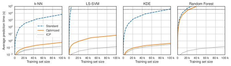
Figure 2: Comparison between the standard and optimized full CP. ICP serves as a baseline for these measurements. Prediction time for one test point w.r.t. the size of training data. Black dashed line is the experiment timeout (10 hours).

6 Bootstrapping methods

Let integer $B>1$ be a hyperparameter, and select a base classifier (e.g., decision tree). In bootstrapping, the training data $Z=\{(x_{1},y_{1}),...,(x_{n},y_{n})\}$ is sampled $B$ times with replacement to produce $B$ bootstrap samples, $Z_{1},...,Z_{B}$. On each sample we fit the base classifier, obtaining an ensemble of $B$ classifiers $(g_{1},...,g_{B})$, which we jointly denote with $f\mathrel{\mathop{\mathchar 58\relax}}X\rightarrow[0,1]^{\ell}$, $\ell=|Y|$.

Classifier $f$ outputs a confidence vector, $f(x)\in[0,1]^{\ell}$, over the labels. The $y$-th element of this vector, denoted by $f^{y}(x)$, is computed as the normalized count of classifiers $g_{i}$ that predict $y$. That is:

$$f^{y}(x)=\frac{1}{B}\text{\#}\{i=1,...,B\,\mathrel{\mathop{\mathchar 58\relax}}\,g_{i}(x)=y\}\quad y\in Y\,.$$

We define the bootstrapping nonconformity measure as:

$$A((x,y);\{(x_{1},y_{1}),...,(x_{n},y_{n})\})=-f^{y}(x)\,.$$

Complexity. Let $T_{g}(n)$ be the time needed to train the base classifier on $n$ training points, and $P_{g}(m)$ its cost to predict $m$ points. Bootstrap CP runs in $\mathcal{O}((T_{g}(n)+P_{g}(1))Bn\ell m)$.

6.1 Optimizing bootstrap CP

Standard bootstrap CP requires training a bootstrap ensemble for each training example $(x_{i},y_{i})$ and one for the test example $(x,y)$; this entails creating, for each example, $B$ bootstrap samples that do not contain that example. The optimization we propose maintains the spirit of bootstrap, although it may lead to different results from the standard version because of changes in the sampling strategy.

We first explain the basic idea for training and prediction, and then improve it with two remarks. Let “$\ast$” be a placeholder for the test point $(x,y)$, which is unavailable during training, and let $Z^{\ast}=Z\cup\{\ast\}$ be the augmented training set. For a number $B^{\prime}>B$ to be later specified, we create $B^{\prime}$ bootstrap samples of $Z^{\ast}$, denoted $\{Z^{\ast}_{1},...,Z^{\ast}_{B^{\prime}}\}$. We continue creating samples until, for every point $(x_{i},y_{i})\in Z^{\ast}$, there are at least $B$ bootstrap samples that do not contain $(x_{i},y_{i})$; that is, we increase the number of samples $B^{\prime}$ until $\text{\#}\{b=1,...,B^{\prime}\,\mathrel{\mathop{\mathchar 58\relax}}\,(x_{i},y_{i})\notin Z^{\ast}_{b}\}\geq B$ for all $(x_{i},y_{i})\in Z^{\ast}$. This ensures that each training point (and the placeholder test point) have at least $B$ bootstrap samples.

Let $E_{i}=\{b=1,...,B^{\prime}\,\mathrel{\mathop{\mathchar 58\relax}}\,(x_{i},y_{i})\notin Z^{\ast}_{b}\}$ be the samples associated with $(x_{i},y_{i})$, and $E=\{b=1,...,B^{\prime}\,\mathrel{\mathop{\mathchar 58\relax}}\,\ast\notin Z^{\ast}_{b}\}$ the ones associated with the (placeholder) test example. In the prediction phase, we compute a prediction for test point $(x,y)$ by using the base classifiers trained on the bootstrap samples in $E$. We make the prediction for a training point $(x_{i},y_{i})$ in the LOO procedure of CP as follows: i) in $E_{i}$’s bootstrap samples, replace the placeholder $\ast$ with the test point $(x,y)$, ii) train the base classifiers on the samples from $E_{i}$ and compute a prediction for $(x_{i},y_{i})$.

Remarks. The procedure explained so far preemptively samples $B$ bootstraps for each point. We apply the following improvements. Because some bootstrap samples $Z^{\ast}_{b}\in E_{i}$ associated with $(x_{i},y_{i})$ do not contain the placeholder $\ast$, in the training phase we: i) pretrain the base classifiers $g_{b}(x)$ on them, and ii) compute their predictions for $(x_{i},y_{i})$. This saves up considerable time in the prediction phase. The optimized bootstrap algorithm is listed in Appendix B.

Complexity. Optimized CP classification for $m$ test points is $\mathcal{O}((T_{g}(n)+P_{g}(1))(1-e^{-1})B\ell m)$, a factor $(1-e^{-1})\approx 0.632$ speed up on the standard one. The speed up of this optimization is not as prominent as our other proposals. However, we suspect one can further improve bootstrap CP for base classifiers that support incremental&decremental learning (Section 9). We leave this to future work.

7 Empirical evaluation

We compare the running time of the original and optimized CP, using ICP as a baseline. We detail hardware, precautions taken to ensure the fidelity of the measurements, and hyperparameters in Appendix E. We instantiate bootstrap CP to Random Forest.

7.1 Comparison between standard and optimized CP

Setup. In our experiments, the data distribution is irrelevant. We generate data for a binary classification problem with $30$ features, by using the make_classification() routine of the scikit-learn library. (In Appendix G, we further compare CP and ICP on the MNIST dataset.)

For every training size $n$, chosen in the space $[10,10^{5}]$, we train the CP with a nonconformity measure, and use it to predict $100$ test points. We set a timeout of 10 hours, which is verified after the prediction of every test point; therefore, the timeout may be exceeded if the prediction for a point has already started. We measure both the training time and the average prediction time for a test point. Each experiment is repeated for 5 different initialization seeds.

Prediction time. Figure 2 shows the comparison between standard and optimized CP. Results confirm the complexity we derived analytically. For 100k training points, the optimized k-NN CP ensures a prediction in 0.63 seconds, whilst the respective unoptimized version takes roughly 2 hours for the same prediction. Since k-NN and Simplified k-NN behave very similarly, results for the latter are in Appendix F. The largest speed up is with LS-SVM: the optimized version has a running time of 0.21 seconds; the standard implementation takes on average more than 24.5 hours for 1 prediction. Our bootstrap CP optimization only gives a marginal improvement over the original implementation. For $n=46415$, optimized Random Forest takes 43 hours for one prediction, the standard one 82 hours.

Comparison with ICP. We use ICP as a baseline. For a parameter $t\in\{1,...,n\}$, ICP trains the nonconformity measure on a subset of $t$ examples, and computes the scores for the remaining $n-t$. We fix $t/n=0.5$.

As expected, results (Figure 2) show that ICP is strictly faster than the optimized CP methods: e.g., when trained on 100k examples, LS-SVM takes 6.68 seconds per prediction, while LS-SVM ICP takes 0.16 seconds; the worst performing is Random Forest, which as seen above improves CP only by a linear factor. Nevertheless, in some cases ICP and optimized CP have the same magnitude: for KDE, ICP takes 0.31 seconds, optimized CP 0.46 seconds. In other words, our CP optimization seems to perform comparably well to ICP on reasonably large datasets.

This reveals a better trade-off between computational-statistical efficiency in conformal inference: if one’s priority is speed, they can use ICP, or other CP alternatives; however, if they can sacrifice computational time, they can get full CP predictions and yet scale to real-world data.

7.2 Training time

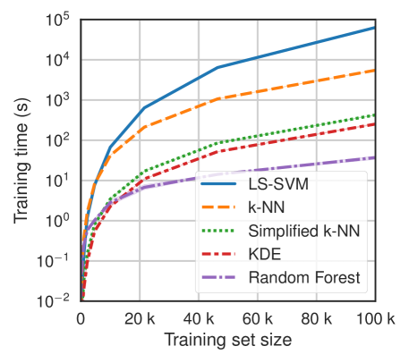
Figure 3: Training time of optimized CP.

CP with the optimized nonconformity measures incurs into a training time, while standard CP does not. We compare the training time of the optimized measures in Figure 3.

We observe that LS-SVM has the highest training time, whilst Random Forest the lowest. We also notice that the training time is a reasonable price to pay in practice. In a batch classification setting with 100k training and 20k test examples, optimized k-NN CP would take 2.2 hours for training and 3.3 hours for prediction. Standard k-NN CP would have no training time, but its prediction routine would run for 9.3 years to obtain the same solution.

It may be possible to speed up our techniques even further via approximate incremental&decremental learning techniques. We leave this to future work (Section 9).

8 Large $Y$ and extension to regression

The classification algorithms for CP (Algorithm 1) and ICP (Algorithm 2) are clearly unfeasible for a very large $Y$: they both require repeating the calculations for each $y\in Y$.

Things are different for regression, where we assume a total order on $Y$. In this case, one can avoid the $\ell=|Y|$ term in the cost of both CP and ICP (Vovk et al., 2005). Indeed, it is possible to find the intervals of $Y$ where the p-value $p_{(x,\hat{y})}$ exceeds $\varepsilon$, without having to try all values $\hat{y}\in Y$. In ICP, this can be done efficiently for general regressors.

As for full CP, this optimization is harder, as one needs to update the intervals of $Y$ for each training point when a new point arrives. Full CP regression was optimized in this sense for k-NN (Papadopoulos et al., 2011), ridge regression (Nouretdinov et al., 2001), and Lasso (Lei, 2019). Ndiaye & Takeuchi (2019) recently proposed a general method leading to approximate but statistically valid CP regressors.

Since the above full CP regression methods do not exploit incremental&decremental ideas, we suspect they can be optimized further. We show this is possible for k-NN.

8.1 Improving the k-NN CP regressor

The full k-NN CP regressor works as follows. Fix an hyperparameter $k>0$. Let $\tilde{y}\in Y$ be a candidate label (not to be defined explicitly) for test object $x$. Define the nonconformity score for the $i$-th training example $(x_{i},y_{i})$ as:

$$\alpha_{i}=\alpha_{i}(\tilde{y})=\mathinner{\!\left\lvert a_{i}+b_{i}\tilde{y}\right\rvert}\,,$$

where, for $i=1,...,n$:

$$a_{i} =\begin{cases}y_{i}-\frac{1}{k}\sum_{j=1}^{k-1}y_{(j)}(x_{i})\quad&\mbox{if $x$ is one of $x_{i}$'s $k$ NNs}\\ y_{i}-\frac{1}{k}\sum_{j=1}^{k}y_{(j)}(x_{i})\quad&\mbox{otherwise}\,,\end{cases}$$

$$b_{i} =\begin{cases}-\frac{1}{k}\quad&\mbox{if $x$ is one of $x_{i}$'s $k$ NNs}\\ 0\quad&\mbox{otherwise}\,;\end{cases}$$

here $y_{(j)}(x_{i})$ is the label of the $j$-th nearest neighbor of $x_{i}$ in the training set $Z\setminus(x_{i},y_{i})$. For the test example $x$, we set $a=-\nicefrac{{1}}{{k}}\sum_{j=1}^{k}y_{(j)}(x)$, $b=1$. The p-value is:

$$p_{(x,\tilde{y})}=\frac{\text{\#}\{i=1,...,n\,\mathrel{\mathop{\mathchar 58\relax}}\,\mathinner{\!\left\lvert a_{i}+b_{i}\tilde{y}\right\rvert}\geq\mathinner{\!\left\lvert a+b\tilde{y}\right\rvert}\}}{n+1}\,.$$

The optimization idea by Papadopoulos et al. (2011) is based on the fact that, in order to find an interval of $Y$ for which $p_{(x,\tilde{y})}>\varepsilon$, it suffices to find the points $\tilde{y}\in Y$ for which $c(\tilde{y})=\alpha_{i}(\tilde{y})-\alpha(\tilde{y})$ changes. This can be done efficiently, by only looking at most at $2n$ points. The time complexity of one prediction is $\mathcal{O}(n^{2}+2n\log(2n))$, where the term $\mathcal{O}(n^{2})$ comes from computing the $k$ nearest neighbors of each training point, and $\mathcal{O}(2n\log(2n))$ comes from sorting the critical points of $c(\tilde{y})$ (required by the above algorithm).

Optimization via incremental&decremental learning. The method by Papadopoulos et al. (2011) can be further improved via the incremental&decremental k-NN algorithm we proposed in this paper. We reduce the $\mathcal{O}(n^{2})$ term as follows. In the training phase, we: i) precompute the pairwise distances of the training points in $Z$, ii) and precompute temporary values $a_{i}^{\prime}$ and $b_{i}^{\prime}$, for $i=1,...,n$. Specifically, we let $a_{i}=y_{i}-\frac{1}{k}\sum_{j=1}^{k}y_{(j)}(x_{i})$ and $b_{i}=0$, as if the (yet unknown) test example $x$ did not contribute to their values. When making a prediction for $x$, we: iii) compute its distance from the elements of $Z$ (takes $\mathcal{O}(n)$), and iv) update those $a_{i}^{\prime}$ and $b_{i}^{\prime}$ such that $x$ is one of the $k$- nearest neighbors of $(x_{i},y_{i})$. Then we proceed as before.

Even in this setting, using an incremental&decremental version of the nonconformity measure enables us to reduce the prediction complexity by almost one order of magnitude. Predicting $m$ test examples reduces from $\mathcal{O}((n^{2}+2n\log(2n))m)$ to $\mathcal{O}(2n\log(2n)m)$.

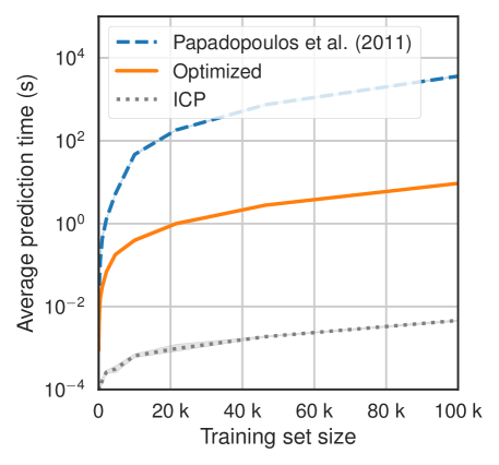
Figure 4: Time comparison of k-NN CP regression: method by Papadopoulos et al. (2011), our optimization, and ICP (baseline).

Empirical evaluation. We compare full k-NN CP regression (Papadopoulos et al., 2011) with our optimization via incremental&decremental learning. As a baseline we use ICP k-NN regression, whose complexity is $\mathcal{O}(tm))$, where $t\in\{2,...,n-1\}$ is the size of the proper training set, and $m$ the number of test points. We generate regression examples from $X\times Y=\mathbb{R}^{30}\times\mathbb{R}$ with scikit-learn’s make_regression() function. We vary $n\in[10,10^{5}]$, and measure the average prediction time across $100$ test points. Each experiment is repeated for $5$ random seeds, and confidence intervals are plotted.

Figure 4 shows that our optimization largely outperforms the previous version of full k-NN CP regression by Papadopoulos et al. (2011); the cost for one prediction with $100$k training points decreases from 1 hour to 9.3 seconds. ICP outperforms both, taking roughly 4.6 ms. We remark, however, that ICP was observed to have a strictly weaker statistical power in regression (Papadopoulos et al., 2011).

Discussion. We expect that our LS-SVM CP optimization (Section 5) can be readily applied to speed up the full CP regressor based on ridge regression (Nouretdinov et al., 2001). We leave this, and the optimization of other CP regressors using incremental&decremental ideas, to future work.

9 Discussion and conclusion

Full CP is computationally expensive because of its main routine (Algorithm 1), which runs a leave-one-out (LOO) procedure on the ML method (nonconformity measure) that it wraps. In this paper, we show that if a nonconformity measure can be designed to learn and unlearn one example efficiently (i.e., it can be trained incrementally&decrementally), this can speed up considerably CP classification. Concretely, we improved k-NN, KDE, and kernel LS-SVM CP classifiers by at least one order magnitude, and bootstrap CP by a linear factor. Furthermore, we exploited these ideas to further optimize k-NN CP regression. Our work makes it feasible to run full CP on large datasets.

We discuss how our optimizations are readily applicable to other tasks (e.g., clustering, change-point detection), and future directions for CP optimization.

Extensions to more learning tasks. In addition to classification and regression, CP is used for tasks such as anomaly detection (Laxhammar & Falkman, 2010), clustering, and sequence prediction (Cherubin & Nouretdinov, 2016). Because all these techniques are based on computing a p-value via Algorithm 1, our optimizations are immediately applicable. For example, conformal clustering (Cherubin et al., 2015) with k-NN CP costs $\mathcal{O}(n^{2}q^{p})$, where $q$ is the length of a square grid constructed around $p$-dimensional training points. With our optimization, the cost becomes $\mathcal{O}(nq^{p})$. (Usually, $p=2$, by using dimensionality reduction.)

CP has applications to online learning (e.g., change-point detection (Vovk et al., 2003)). At step $n+1$, the algorithm trains on examples $\{(x_{i},y_{i})\}_{i=1}^{n}$, makes a prediction for $x_{n+1}$, and learns the true label $y_{n+1}$. Adapting our optimizations to this setting is trivial: it suffice to incrementally learn the new example $(x_{n+1},y_{n+1})$ after prediction, which is efficient for k-NN, KDE and LS-SVM. This has a considerable speed-up. For example, an IID test by Vovk et al. (2003), which has further applications to feature selection (Cherubin et al., 2018), requires to incrementally compute a p-value for the $(n+1)$-th point given $\{(x_{i},y_{i})\}_{i=1}^{n}$. With k-NN CP, this costs $\mathcal{O}(n^{3})$; our method reduces it to $\mathcal{O}(n^{2})$ (Appendix C). Unfortunately, this is not efficient for bootstrap; we leave its further optimization to future work.

The umbrella of conformal inference also includes methods such as Venn Predictors (VP), which give analogous guarantees to CP, but for the calibration of probabilistic predictions. Future work may investigate whether VP can be optimized with similar techniques to the ones we proposed.

Boosting and gradient descent. We hope our work will inspire optimization techniques for more nonconformity measures. We foresee as particularly challenging the optimization of methods such as boosting and gradient descent. For both techniques, the contribution of a training example depends on previous examples. Hence, unlearning an example has a high cost, as it requires updating the contributions of all the examples that came after. We suggest recent work on unlearning methods may help to achieve this goal.

Approximations. Another natural avenue is to use approximate incremental&decremental learning techniques. For example, by bounding the contribution of each point it may be possible to achieve very computationally efficient methods with little cost on statistical efficiency.

Exploiting multiple CPUs, GPUs. A further direction is to study how to exploit a GPU or multiple CPUs to speed up CP. Towards this goal, we conducted a preliminary comparison between parallel and sequential implementations of CP and optimized CP (Appendix H); CP and optimized CP are parallelized in the same way. Results show that, for a small dataset (5k examples) standard CP benefits from parallelization, while optimized CP does not substantially. Surprisingly, in this case optimized k-NN is even faster without parallelization, although it does benefit for larger datasets. More research is needed to determine the best parallelization strategies for CP, both from an algorithmic and implementational level. We leave this, and the study of GPUs for CP, to future work.

Appendix A Details on CP and CP-inspired methods for classification

In the following table, $\ell=|Y|$, $T_{A}(n)$ is the training complexity on $n$ examples of the nonconformity measure $A$, $P_{A}(m)$ is its running time for predicting $m$ examples, $n$ and $m$ is respectively the number of training and test examples. In ICP and aggregated CP, $t\in\{1,...,n\}$ is the size of the proper training set. In cross and aggregated CP, $K\in\{2,...,n\}$ is a tuning parameter (number of folds).

	Train + Calibrate	Predict
CP	N/A	$\mathcal{O}((T_{A}(n)+P_{A}(1))n\ell m)$
ICP	$\mathcal{O}(T_{A}(t)+P_{A}(n-t))$	$\mathcal{O}((P_{A}(1)+n-t)\ell m)$
Cross CP	$\mathcal{O}((T_{A}((\nicefrac{{K-1}}{{K}})n)+P_{A}(\nicefrac{{n}}{{K}}))K)$	$\mathcal{O}((P_{A}(1)+\nicefrac{{n}}{{K}})K\ell m)$
Aggregated CP	$\mathcal{O}((T_{A}(t)+P_{A}(n-t))K)$	$\mathcal{O}((P_{A}(1)+n-t)K\ell m)$

ICP. Algorithm 2 describes the algorithms for calibrating and computing a p-value with ICP. In the training phase, ICP trains the nonconformity measure $A$ on the proper training set, $\{(x_{1},y_{1}),...,(x_{t},y_{t})\}$, and uses $A$ to compute the nonconformity scores on the calibration set $\{(x_{t+1},y_{t+1}),...,(x_{n},y_{n})\}$ (Lines 1-6). Similarly to CP classification, an ICP classifier computes a p-value for every $\hat{y}\in Y$ by running COMPUTE_PVALUE() (Lines 8-11); differently from CP, the p-value is only based on the nonconformity scores computed during calibration and the one for the test object.

1	calibrate$(x,y,\{(x_{1},y_{1}),...,(x_{n},y_{n})\},t,A)$
2	$Z_{train}=\{(x_{1},y_{1}),...,(x_{t},y_{t})\}$
3	$Z_{calib}=\{(x_{t+1},y_{t+1}),...,(x_{n},y_{n})\}$
4	for $i$ in t+1, …, n
5	$\alpha_{i}=A((x_{i},y_{i});Z_{train})$
6	return $A(\cdot;Z_{train}),\{\alpha_{t+1},...,\alpha_{n}\}$
7
8	compute_pvalue$(x,\hat{y},A(\cdot;Z_{train}),\{\alpha_{t+1},...,\alpha_{n}\})$
9	$\alpha=A((x,\hat{y});Z_{train})$
10	$p_{(x,\hat{y})}=\frac{\text{\#}\{i=t+1,...,n\,\mathrel{\mathop{\mathchar 58\relax}}\,\alpha_{i}\geq\alpha\}+1}{n-t+1}$
11	return $p_{(x,\hat{y})}$

Algorithm 2 Inductive Conformal Prediction: computing a p-value for $(x,\hat{y})$

CP alternatives. Algorithms of aggregated CP (Carlsson et al., 2014), cross CP (Vovk, 2015), CV+ and jackknife+ (Barber et al., 2019) can be found in the respective references. Note that CV+ and jackknife+, albeit originally designed for regression, can be extended to classification tasks (Appendix D in (Gupta et al., 2019)).

Appendix B Details on optimized nonconformity measures

B.1 LS-SVM

An LS-SVM model $w$ is learned as a solution of:

$$w=\arg\min_{w\in\mathbb{R}^{h}}\rho||w||^{2}+\sum_{i=1}^{n}(w^{\top}\phi(x_{i})-y_{i})^{2}\,,$$

for regularization parameter $\rho$. The closed-form solution to this is:

$$w^{*}=\Phi[\Phi^{\top}\Phi+\rho I_{n}]^{-1}Y\,,$$

where $\Phi=[\phi(x_{1}),...,\phi(x_{n})]$, $Y=\{y_{1},...,y_{n}\}$, and $I_{n}$ is the identity matrix of size $n\times n$.

The incremental&decremental learning method by Lee et al. (2019) requires storing an auxiliary matrix:

$$C=\Phi[\Phi^{\top}\Phi+\rho I_{n}]^{-1}\Phi^{\top}\,.$$

A description of how to learn incrementally or unlearn an example follows (Lee et al., 2019).

Incremental learning of one example. To learn $(x_{n+1},y_{n+1})$, update the model as follows:

$$w_{new} =w+\frac{(C-I_{q})\phi(x_{n+1})\left(\phi(x_{n+1})^{\top}w-y_{n+1}\right)}{\phi(x_{n+1})^{\top}\phi(x_{n+1})+\rho-\phi(x_{n+1})^{\top}C\phi(x_{n+1})}$$

$$C_{new} =C+\frac{(C-I_{q})\phi(x_{n+1})\phi(x_{n+1})^{\top}(C-I_{q})}{\phi(x_{n+1})^{\top}\phi(x_{n+1})+\rho-\phi(x_{n+1})^{\top}C\phi(x_{n+1})}\,.$$

Where $q$ is the size of the kernel space.

Decremental learning of one example. To unlearn $(x_{i},y_{i})$, update the model as follows:

$$w_{new} =w-\frac{(C-I_{q})\phi(x_{i})\left(\phi(x_{i})^{\top}w-y_{i}\right)}{-\phi(x_{i})^{\top}\phi(x_{i})+\rho+\phi(x_{i})^{\top}C\phi(x_{i})}$$

$$C_{new} =C-\frac{(C-I_{q})\phi(x_{i})\phi(x_{i})^{\top}(C-I_{q})}{-\phi(x_{i})^{\top}\phi(x_{i})+\rho+\phi(x_{i})^{\top}C\phi(x_{i})}\,.$$

B.2 Bootstrap algorithm

Algorithm 3 shows the entire optimized bootstrap CP algorithm. In the training phase, $B^{\prime}$ bootstrap samples are generated, and for some of them (those that do not contain the placeholder “$\ast$”) a classifier is trained. To compute a p-value for example $(x,\hat{y})$, the remaining classifiers are trained (after replacing “$\ast$” with $(x,\hat{y})$), and the predictions are computed as usual. A full implementation is provided in the code attached to this submission.

1	train$(\{(x_{1},y_{1}),...,(x_{n},y_{n})\},B)$
2	$Z^{\ast}=Z\cup\{\ast\}$                                // “$\ast$” is a placeholder for the test example $(x,\hat{y})$
3	$E_{1},...,E_{n},E\leftarrow\{\}$
4
5	// Associate at least $B$ bootstrap samples to each training example and to “$\ast$”
6	for $B^{\prime}$ in 1, 2, 3, …
7	$Z^{\ast}_{B^{\prime}}\leftarrow$ sample $|Z^{\ast}|$ examples from $Z^{\ast}$ with replacement
8	for $i=1,...,n$
9	if $(x_{i},y_{i})\notin Z^{\ast}_{B^{\prime}}$
10	Insert $Z^{\ast}_{B^{\prime}}$ into $E_{i}$
11	if $\ast\notin Z^{\ast}_{B^{\prime}}$
12	Insert $Z^{\ast}_{B^{\prime}}$ into $E$
13	if $|E|\geq B$ and $|E_{i}|\geq B$ for all $i=1,...,n$
14	exit for loop
15
16	// Pretraining for bootstrap samples that do not contain “$\ast$”
17	for $i=1,...,n$
18	for $Z_{b}\in E_{i}$
19	if $\ast\notin Z_{b}$
20	Train classifier $g$ on $Z_{b}$, and replace element $Z_{b}$ with $g(x)$ in $E_{i}$
21
22	// Pretraining for placeholder “$\ast$”. Note: by construction, no element of $E$ contains “$\ast$”
23	for $Z_{b}$ in $E$
24	Train classifier $g$ on $Z_{b}$, and replace element $Z_{b}$ with $g(x)$ in $E$
25
26	return $E_{1},...,E_{n},E$
27
28	compute_pvalue$((x,\hat{y}),E_{1},...,E_{n},E)$
29	// Compute the nonconformity scores for the training examples
30	for $i=1,...,n$
31	$\alpha_{i}=0$
32	for $e\in E_{i}$
33	if $e$ is a pretrained classifier, call it $g(x)$
34	$\alpha_{i}=\alpha_{i}-g^{\hat{y}}(x)$
35	else ($e$ is a bootstrap sample $Z_{b}$ that contains “$\ast$”)
36	Replace “$\ast$” with $(x,\hat{y})$ in $Z_{b}$
37	Train classifier $g$ on $Z_{b}$
38	$\alpha_{i}=\alpha_{i}-g^{\hat{y}}(x)$
39
40	// Compute nonconformity score for the test example
41	$\alpha=0$
42	for $g(x)\in E$
43	$\alpha=\alpha-g^{\hat{y}}(x)$
44
45	// Compute p-value
46	$p_{(x,\hat{y})}=\frac{\text{\#}\{i=1,...,n\,\mathrel{\mathop{\mathchar 58\relax}}\,\alpha_{i}\geq\alpha\}+1}{n+1}$
47
48	return $p_{(x,\hat{y})}$

Algorithm 3 Optimized bootstrap CP algorithm.

Appendix C Time complexity derivations

C.1 Simplified k-NN and k-NN

Standard. For simplicity, we only describe the complexity of Simplified k-NN; the complexity of k-NN is identical to the one derived for Simplified k-NN up to a linear factor.

Let us define a routine, best_k(A), which returns the $k$ smallest elements of a set $A$ of size $n$. In our work, we instantiate this to Introselect, which runs in $\mathcal{O}(n)$ worst-case.

The cost for computing the nonconformity measure $A((x,y);\{(x_{1},y_{1}),...,(x_{n},y_{n})\})$ for one example $(x,y)$ requires computing the distances from $x$ to the training points $\{(x_{1},y_{1}),...,(x_{n},y_{n})\}$, and selecting the $k$ best. Overall, by using best_k(A), this amounts to $\mathcal{O}(n)$. From the time complexity of CP classification (Section 2), we get that running CP with the (Simplified) k-NN nonconformity measure to predict $m$ test examples takes $\mathcal{O}(n^{2}\ell m)$.

Optimized. In the training phase, we precompute the distances and preliminary scores for the $n$ training examples ($\mathcal{O}(n^{2})$), and store both. To compute the nonconformity score $A$ for one example $(x_{i},y_{i})$ in the prediction phase, we only need to compute its distance from the test example $(x,y)$, and update the provisional score $\alpha_{i}$ if this distance is smaller than one of the best $k$ distances. This has cost $\mathcal{O}(1)$. The cost of CP classification with the optimized measure is therefore $\mathcal{O}(n\ell m)$.

C.2 KDE

Standard. Let $P_{K}$ be the time to compute the kernel on 1 input. To compute the nonconformity score, we repeat this operation for all the training points ($\mathcal{O}(P_{K}n)$). Hence the cost of KDE CP classification is: $\mathcal{O}(P_{K}n\ell m)$.

Optimized. The training costs of this algorithm is $\mathcal{O}(P_{K}n^{2})$. The cost for updating one nonconformity score with our optimization is $\mathcal{O}(P_{K})$. Therefore, the cost of optimized KDE CP for classification is $\mathcal{O}(P_{K}n\ell m)$.

C.3 LS-SVM

Standard. The running time of LS-SVM CP is dominated by training LS-SVM. Let $\mathcal{O}(n^{\omega})$, $\omega\in[2,3]$ be this training cost. Then, CP classification is $\mathcal{O}(n^{\omega+1}\ell m)$.

Optimized. Training the optimized algorithm has the same cost as training standard LS-SVM, $\mathcal{O}(n^{\omega})$. Let $q$ be the dimensionality of the objects after feature mapping $\phi(x)$. To compute the nonconformity score for an example $(x_{i},y_{i})$, we: i) update the model with the test example by using the method by Lee et al. (2019), ii) make a prediction for $(x_{i},y_{i})$. The first operation has cost $\mathcal{O}(q^{3})$), the second one requires $n$ kernel evaluations and $\mathcal{O}(q)$ for the dot product. Therefore, predicting with optimized LS-SVM is $\mathcal{O}(q^{3}n\ell m)$.

C.4 Bootstrap

Standard. Let $T_{g}(n)$ be the time needed to train the base classifier on $n$ training points, and $P_{g}(m)$ its running time when computing a prediction for $m$ points. To compute the bootstrap nonconformity measure once we need to train $B$ base classifiers and run each one to compute a prediction. This amounts to $\mathcal{O}((T_{g}(n)+P_{g}(1))B)$. The overall complexity of bootstrap CP classification is $\mathcal{O}((T_{g}(n)+P_{g}(1))Bn\ell m)$.

Optimized. During the training phase, and for each training point, we will need to train (and make predictions for), in expectation, $BPr\left(\ast\notin Z_{b}\right)$, where $Pr\left(\ast\notin Z_{b}\right)$ is the probability that an example (“$\ast$”, in this case) is not contained in a bootstrap sample of $Z^{\ast}$ with replacement. It is easy to see that $BPr\left(\ast\notin Z_{b}\right)=B(1-\nicefrac{{1}}{{n+1}})^{n+1}\approx Be^{-1}$. If we repeat the argument for all training examples, the training phase (Lines 1-26 in Algorithm 3) takes time $(T_{g}(n)+P_{g}(1))Be^{-1}n$.

Computing the p-value for one point is obtained as the complement of the probability, $(T_{g}(n)+P_{g}(1))B(1-e^{-1})n$. This is a linear factor $(1-e^{-1})\approx 0.632$ the speed of the original one. Overall, CP classification takes $(T_{g}(n)+P_{g}(1))B(1-e^{-1})n\ell m$ for classifying $m$ test examples in $\ell$ labels.

Remark. The actual complexity of optimized bootstrap CP is generally lower than the one derived above. Indeed, in the above calculations we assumed that each bootstrap sample is used for just one point; however, some bootstrap samples (and respective classifiers) are in fact shared among several training points. Therefore, the effective number of classifiers one needs to train is only $B^{\prime}$, and not $Bn$. We show the relation between $B$ and $B^{\prime}$ in Figure 5, which indicates that $B^{\prime}<Bn$.

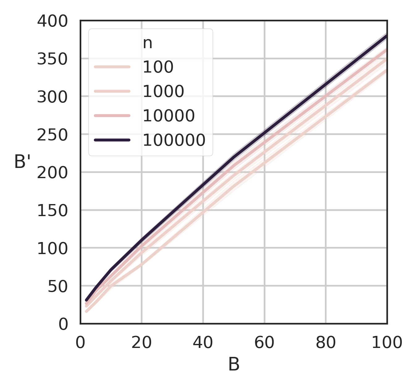
Figure 5: Relation between $B$, $n$, and $B^{\prime}$ for the optimized bootstrap CP algorithm.

C.5 IID test by Vovk et al. (2003)

Vovk et al. (2003) introduced an online algorithm for testing the exchangeability (or IID-ness) of a sequence of observations. At step $n$, having observed $\{x_{1},...,x_{n}\}$, it computes a p-value (Algorithm 1) for a new observation $x_{n+1}$. On the basis of the computed p-values, the test derives exchangeability martingales which can be used as the basis of an hypothesis test.

Suppose we use the k-NN nonconformity measure. Computing one p-value using standard k-NN CP is $\mathcal{O}(n^{2})$. Since standard CP does not have any way of exploiting previous computations, the p-values have to be computed independently. The cost of processing $n$ observations is $1^{2}+2^{2}+...+n^{2}=\sum_{i=1}^{n}i^{2}=\frac{1}{6}n(n+1)(2n+1)$. Hence, $\mathcal{O}(n^{3})$.

When using the optimized k-NN CP, the cost of computing one p-value for $x_{n+1}$ given $n$ training examples is $\mathcal{O}(n)$; this includes the cost of training on the new observation. This means the cost of computing $n$ p-values incrementally, as required by the IID test, is $1+2+...+n=\frac{n(n+1)}{2}$. That is, $\mathcal{O}(n^{2})$.

Appendix D Memory costs

A standard CP implementation requires storing the entire training data $Z$, which has cost $\mathcal{O}(np)$, where $n$ is the number of examples, $p$ their dimensionality. In addition to this cost, the optimized CP versions we introduced have the following requirements.

(Simplified) k-NN. Store, for every training point: i) the largest among the best $k$ distances, ii) the provisional score. This has cost $\mathcal{O}(n)$, negligible w.r.t. the $\mathcal{O}(np)$ already required by CP.

KDE. Store the $n$ preliminary scores, $\mathcal{O}(n)$, which is negligible w.r.t. $\mathcal{O}(np)$.

LS-SVM. requires storing the model, $w\in\mathbb{R}^{q}$, and an auxiliary $q\times q$ matrix required by the method by Lee et al. (2019), where $q$ is the dimensionality of the kernel space. Including the cost of standard CP, the memory used is $\mathcal{O}(np+q^{2})$.

Bootstrap. In the optimized algorithm, we create $B^{\prime}$ bootstrap samples. Of them, on average $B^{\prime}e^{-1}$ do not contain the placeholder $\ast$; we can therefore train them and compute a prediction for them (Lines 16-24). Storing these predictions has cost $\mathcal{O}(B^{\prime}e^{-1})$. For the remaining ones, we need record the indices pointing to the augmented dataset $Z^{\ast}$, so that in the test phase we can reconstruct the bootstrap samples. We store $n$ indices for each, totaling a memory cost of $\mathcal{O}(B^{\prime}(1-e^{-1})n)$. The overall cost of bootstrap CP is $\mathcal{O}(np+B^{\prime}(1-e^{-1})n)$. The relation between $B^{\prime}$, $B$, and $n$ is shown in Figure 5.

Appendix E Experiment details

Hardware and multiprocessing. We conduct our experiments on a 2x Intel Xeon E5-2680 v3 (48 threads) machine, with 256 GB RAM. In these experiments, each time measurement is performed on a single core. We limit the number of cores available for the experiment, so as to prevent time measurements from being affected by other running processes (e.g., kernel tasks). We prevent numpy from automatically parallelizing matrix calculations.

Hyperparameters. We use the following hyperparameters for the nonconformity measures.

Method	Hyperparameters
Simplified k-NN & k-NN	Euclidean distance, $k=15$.
KDE	Gaussian kernel. Bandwidth $h=1$.
LS-SVM	Linear kernel, $\rho=1$.
Bootstrapping	We instantiate bootstrapping to Random Forest, with $B=10$ classifiers. Each classifier, a decision tree, is allowed to grow up to depth 10, and to select among $\sqrt{p}$ of features for a split, where $p$ is the dimensionality of $X$.

When measuring time w.r.t. the training size $n$, we vary $n$ in the space $[10,10^{5}]$, by evenly separating $13$ values on a log scale.

Appendix F Simplified k-NN results

Due to lack of space, Figure 2 did not include results for Simplified k-NN. Figure 6 compares k-NN and Simplified k-NN, showing that they are very similar – indeed, their asymptotic time complexities are also identical.

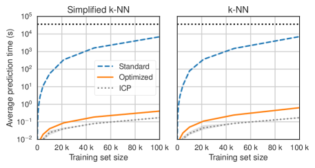
Figure 6: Comparison between standard and optimized k-NN and Simplified k-NN. ICP is used as a baseline. Prediction time for one test point w.r.t. the size of training data. Black dashed line is the experiment timeout (10 hours).

Appendix G Experiments on MNIST

We conduct experiments on the MNIST dataset (LeCun et al., 2010), which includes 60k training examples and 10k test examples. This dataset’s records have a much higher dimensionality than those considered in our previous experiments: each object is a 28x28 pixel matrix (784 features in total). Furthermore, this is a 10-label classification setting; the number of labels strongly penalizes CP (and ICP), although this is an irreducible cost if we make no assumptions on $Y$ (Section 8). (Fisch et al. (2021) recently made some developments w.r.t. this particular aspect.)

Time costs. We run standard and optimized CP on this dataset, by using the original training-test split. We do not include LS-SVM in this set of experiments, as it is specific to binary classification (although it could be extended by using e.g. a one-vs-all approach).

	CP	Optimized CP	ICP
NN	0s / T(1)	34m 5s / 7h 9m	22m 58s / 2h 38m
SimplifiedKNN	0s / T(1)	29s / 4h 36m	3m 47s / 1h 38m
KNN	0s / T(0)	34m 17s / 7h 21m	20m 25s / 2h 29m
KDE	0s / T(1)	1h 17m / 29h 13m	1h 30m / 6h 13m
RandomForest	0s / T(0)	48s / T(0)	21s / 1h 25m

Table 2: MNIST evaluation. Each entry reports training/prediction time for 60k training and 10k test points. $T(p)$ indicates that the timeout (48h) was reached before completing all the predictions, and that $p$ predictions were made by then.

Table 2 indicates that the advantage of using optimized CP w.r.t. standard CP is substantial; in particular, for the fastest nonconformity measures, standard CP could make just 1 prediction (out of 10k test points) within the 48h timeout limit. Results also suggest that exact optimized CP is a practical alternative to ICP; for example, optimized Simplified k-NN CP run in 4.3 hours, while ICP with the same nonconformity measure run in 1.6 hours. Unfortunately, optimized Random Forest was unable to make any predictions within the 48h timeout; we hope this method can be further optimized in the future. Finally, we observe that optimized CP KDE was substantially worse than ICP; the reason is that, for the experiments on MNIST, we used arbitrary precision math to make KDE numerically stable – something that can be improved upon.

Statistical Efficiency of CP and ICP. As a byproduct of the above experiment, we are able to compare CP and ICP on the basis of their statistical power (efficiency). Note that an analysis on such a large dataset would not have been possible without using our CP optimizations.

We compare CP and ICP in terms of their fuzziness on the MNIST test set. The fuzziness of a set of p-values $\{p_{(x,y)}\}_{y\in Y}$, returned by CP or ICP as the prediction for test object $x$, is the average of the p-values excluding the largest one:

$$\sum_{y\in Y}p_{(x,y)}-\max_{y}p_{(x,y)}\,.$$

A smaller fuzziness indicates better performance (Vovk et al., 2016). We use a Welch one-sided statistical test for the null hypothesis $H_{0}$: “ICP has a smaller fuzziness (i.e., it is better) than CP”. We reject the null hypothesis for a p-value $<0.01$.

The table below indicates the fuzziness of the evaluated techniques for the MNIST dataset. An asterisk * indicates statistical significance. Random Forest CP was excluded, as it did not return predictions within the timeout (Table 2).

Results demonstrate CP is consistently better w.r.t. fuzziness than ICP. However, we observe that future work is needed to compare CP and ICP under various conditions (e.g., umbalanced data, distribution shift, …). Our optimizations make this analysis feasible.

	CP	ICP
NN	0.00047 $\pm$ 0.00105*	0.00065 $\pm$ 0.00143
Simplified k-NN	0.04998 $\pm$ 0.07151*	0.05684 $\pm$ 0.07744
k-NN	0.00066 $\pm$ 0.00125*	0.00098 $\pm$ 0.00174
KDE	0.04494 $\pm$ 0.07005*	0.16791 $\pm$ 0.11729

Appendix H Does multiprocessing help?

We consider a multiprocessing implementation for CP classification. The CP implementation parallelizes Algorithm 1, which is run for every label and test point. Standard and optimized CP are parallelized in the same way. For the parallel versions, we employ a Python Pool of processes, as shown in the code included in the supplementary material.

We used the 48 threads machine described in Section 7, and made all the cores available for multiprocessing. We generated a dataset of size 1000, split it into training (%70) and test sets, and timed the sequential and parallel versions. Due to the high complexity of standard CP, we could not evaluate this for larger datasets. We report the measurements collected over 5 runs.

Results (Table 3) indicate that CP with standard nonconformity measures always benefits from parallelization, bringing at least one order of magnitude speed up. Conversely, optimized nonconformity measures give a mixed picture: except for LS-SVM and Random Forest, parallelization only brings mild improvements. Surprisingly, optimized k-NN CP is faster than the respective parallel version.

After this observation, we repeated the experiment just for optimized k-NN CP, for a dataset of 100k examples. In this case, parallelization indeed helps: prediction takes 1 hour for the parallel version, 3.5 hours for the sequential one. We conclude that the benefit of multiprocessing exists, but only for large datasets. We suspect this is due to the overhead of creating new processes, and that it can be further optimized in the future by working on the implementational details.

Table 3: Time comparison of sequential and parallel implementations, based on a dataset of 1000 examples with $30$ features each. Time is measured in seconds.

		CP	CP Parallel
Standard	Simplified k-NN	74.60 $\pm$ 1.46	3.95 $\pm$ 0.18
	k-NN	82.14 $\pm$ 1.29	4.11 $\pm$ 0.17
	KDE	138.48 $\pm$ 1.49	6.66 $\pm$ 0.28
	LS-SVM	8852.18 $\pm$ 27.46	624.74 $\pm$ 2.58
	Random Forest	5061.67 $\pm$ 310.75	225.75 $\pm$ 4.41
Optimized	Simplified k-NN	1.29 $\pm$ 0.01	0.43 $\pm$ 0.05
	k-NN	1.60 $\pm$ 0.27	9.04 $\pm$ 0.33
	KDE	1.35 $\pm$ 0.14	0.41 $\pm$ 0.00
	LS-SVM	8.47 $\pm$ 0.58	0.76 $\pm$ 0.01
	Random Forest	2409.59 $\pm$ 546.21	110.32 $\pm$ 32.50

References

- Barber et al. (2019) Barber, R. F., Candes, E. J., Ramdas, A., and Tibshirani, R. J. Predictive inference with the jackknife+. arXiv preprint arXiv:1905.02928, 2019.
- Carlsson et al. (2014) Carlsson, L., Eklund, M., and Norinder, U. Aggregated conformal prediction. In IFIP International Conference on Artificial Intelligence Applications and Innovations, pp. 231–240. Springer, 2014.
- Carlsson et al. (2017) Carlsson, L., Bendtsen, C., and Ahlberg, E. Comparing performance of different inductive and transductive conformal predictors relevant to drug discovery. In Conformal and Probabilistic Prediction and Applications, pp. 201–212, 2017.
- Cauwenberghs & Poggio (2001) Cauwenberghs, G. and Poggio, T. Incremental and decremental support vector machine learning. In Advances in neural information processing systems, pp. 409–415, 2001.
- Cherubin & Nouretdinov (2016) Cherubin, G. and Nouretdinov, I. Hidden markov models with confidence. In Symposium on Conformal and Probabilistic Prediction with Applications, pp. 128–144. Springer, 2016.
- Cherubin et al. (2015) Cherubin, G., Nouretdinov, I., Gammerman, A., Jordaney, R., Wang, Z., Papini, D., and Cavallaro, L. Conformal clustering and its application to botnet traffic. In International Symposium on Statistical Learning and Data Sciences, pp. 313–322. Springer, 2015.
- Cherubin et al. (2018) Cherubin, G., Baldwin, A., and Griffin, J. Exchangeability martingales for selecting features in anomaly detection. In Conformal and Probabilistic Prediction and Applications, pp. 157–170. PMLR, 2018.
- Fisch et al. (2021) Fisch, A., Schuster, T., Jaakkola, T., and Barzilay, R. Efficient conformal prediction via cascaded inference with expanded admission. In International Conference on Learning Representations (ICLR), 2021.
- Fukunaga & Hummels (1989) Fukunaga, K. and Hummels, D. M. Leave-one-out procedures for nonparametric error estimates. IEEE Transactions on Pattern Analysis and Machine Intelligence, 11(4):421–423, 1989.
- Gupta et al. (2019) Gupta, C., Kuchibhotla, A. K., and Ramdas, A. K. Nested conformal prediction and quantile out-of-bag ensemble methods. arXiv preprint arXiv:1910.10562, 2019.
- Hamerly & Speegle (2010) Hamerly, G. and Speegle, G. Efficient model selection for large-scale nearest-neighbor data mining. In British National Conference on Databases, pp. 37–54. Springer, 2010.
- Laxhammar & Falkman (2010) Laxhammar, R. and Falkman, G. Conformal prediction for distribution-independent anomaly detection in streaming vessel data. In Proceedings of the first international workshop on novel data stream pattern mining techniques, pp. 47–55, 2010.
- LeCun et al. (2010) LeCun, Y., Cortes, C., and Burges, C. Mnist handwritten digit database. ATT Labs [Online]. Available: http://yann.lecun.com/exdb/mnist, 2, 2010.
- Lee et al. (2019) Lee, W.-H., Ko, B. J., Wang, S., Liu, C., and Leung, K. K. Exact incremental and decremental learning for LS-SVM. In 2019 IEEE International Conference on Image Processing (ICIP), pp. 2334–2338. IEEE, 2019.
- Lei (2019) Lei, J. Fast exact conformalization of the lasso using piecewise linear homotopy. Biometrika, 106(4):749–764, 2019.
- Lei et al. (2018) Lei, J., G’Sell, M., Rinaldo, A., Tibshirani, R. J., and Wasserman, L. Distribution-free predictive inference for regression. Journal of the American Statistical Association, 113(523):1094–1111, 2018.
- Linusson et al. (2014) Linusson, H., Johansson, U., Boström, H., and Löfström, T. Efficiency comparison of unstable transductive and inductive conformal classifiers. In IFIP International Conference on Artificial Intelligence Applications and Innovations, pp. 261–270. Springer, 2014.
- Makili et al. (2013) Makili, L., Vega, J., and Dormido-Canto, S. Incremental support vector machines for fast reliable image recognition. Fusion Engineering and Design, 88(6-8):1170–1173, 2013.
- Ndiaye & Takeuchi (2019) Ndiaye, E. and Takeuchi, I. Computing full conformal prediction set with approximate homotopy. arXiv preprint arXiv:1909.09365, 2019.
- Nouretdinov et al. (2001) Nouretdinov, I., Melluish, T., and Vovk, V. Ridge regression confidence machine. In ICML, pp. 385–392. Citeseer, 2001.
- Papadopoulos et al. (2002) Papadopoulos, H., Proedrou, K., Vovk, V., and Gammerman, A. Inductive confidence machines for regression. In European Conference on Machine Learning, pp. 345–356. Springer, 2002.
- Papadopoulos et al. (2011) Papadopoulos, H., Vovk, V., and Gammerman, A. Regression conformal prediction with nearest neighbours. Journal of Artificial Intelligence Research, 40:815–840, 2011.
- Tsai et al. (2014) Tsai, C.-H., Lin, C.-Y., and Lin, C.-J. Incremental and decremental training for linear classification. In Proceedings of the 20th ACM SIGKDD international conference on Knowledge discovery and data mining, pp. 343–352, 2014.
- Vovk (2015) Vovk, V. Cross-conformal predictors. Annals of Mathematics and Artificial Intelligence, 74(1-2):9–28, 2015.
- Vovk et al. (2003) Vovk, V., Nouretdinov, I., and Gammerman, A. Testing exchangeability on-line. In Proceedings of the 20th International Conference on Machine Learning (ICML-03), pp. 768–775, 2003.
- Vovk et al. (2005) Vovk, V., Gammerman, A., and Shafer, G. Algorithmic learning in a random world. Springer Science & Business Media, 2005.
- Vovk et al. (2016) Vovk, V., Fedorova, V., Nouretdinov, I., and Gammerman, A. Criteria of efficiency for conformal prediction. In Symposium on Conformal and Probabilistic Prediction with Applications, pp. 23–39. Springer, 2016.
- Vovk et al. (2017) Vovk, V., Shen, J., Manokhin, V., and Xie, M.-g. Nonparametric predictive distributions based on conformal prediction. In Conformal and Probabilistic Prediction and Applications, pp. 82–102. PMLR, 2017.