A FORECAST OF THE SENSITIVITY ON THE MEASUREMENT OF THE OPTICAL DEPTH TO REIONIZATION WITH THE GROUNDBIRD EXPERIMENT

Abstract

We compute the expected sensitivity on measurements of optical depth to reionization for a ground-based experiment at Teide Observatory. We simulate polarized partial sky maps for the GroundBIRD experiment at the frequencies 145 and 220 GHz. We perform fits for the simulated maps with our pixel-based likelihood to extract the optical depth to reionization. The noise levels of polarization maps are estimated as 110 $\mu\mathrm{K~{}arcmin}$ and 780 $\mu\mathrm{K~{}arcmin}$ for 145 and 220 GHz, respectively, by assuming a three-year observing campaign and sky coverages of 0.537 for 145 GHz and 0.462 for 220 GHz. Our sensitivities for the optical depth to reionization are found to be $\sigma_{\tau}$=0.030 with the simulated GroundBIRD maps, and $\sigma_{\tau}$=0.012 by combining with the simulated QUIJOTE maps at 11, 13, 17, 19, 30, and 40 GHz.

1 Introduction

A model of rapid accelerated expansion of the early universe (Starobinsky, 1980; Guth, 1981; Sato, 1981; Albrecht & Steinhardt, 1982; Linde, 1982), required in order to resolve the horizon and flatness problems of the standard model of cosmology, predicts the production of two distinct polarized patterns in the cosmic microwave background (CMB) radiation due to density fluctuation and the production of primordial gravitational waves (Kamionkowski et al., 1997a; Seljak & Zaldarriaga, 1997; Zaldarriaga & Seljak, 1997; Kamionkowski et al., 1997b). Along with this possible inflationary expansion scenario of the early universe, the standard model of cosmology, or a spatially-flat six-parameter model of the universe ($\Lambda$CDM), having a cosmological constant and dark matter as dominant forms of the energy density in the universe at present, agrees remarkably well with observational data to date. In both cases, the CMB polarization plays a key role in discovering the physics of the early universe. Among six parameters in the $\Lambda$CDM model of the standard cosmology, the optical depth to reionization ($\tau$), a dimensionless quantity that provides a measure of the line-of-sight free-electron opacity to CMB radiation, has important cosmological implications.

Of the six parameters in the $\Lambda$CDM model mentioned, $\tau$ is the only one that is measured with sensitivity worse than 1% at present, $\tau=0.054\pm 0.007$ (Planck Collaboration, 2020). This measurement also constrains the sum of the neutrino masses, one of the critical parameters in describing the evolution of the early universe. We can determine the sum of the neutrino masses by comparing the primordial amplitude of CMB, $A_{s}$, and the amplitude of CMB at small scales. It gives, however, the combination of $A_{s}e^{-\tau}$ only, and thus a precise measurement of $\tau$ is required to better constrain the neutrino mass via $A_{s}$ (Allison et al., 2015; Bryan et al., 2018; Ferraro & Smith, 2018; Planck Collaboration, 2020).

At large angular scales in the polarization power spectrum of the CMB ($\ell\lesssim 10$ where $\ell$ is the multipole index in the angular power spectrum), anisotropies are created by the rescattering of the local temperature quadrupole (Zaldarriaga, 1997; Planck Collaboration, 2020). These lead to a “bump” today in the large-scale polarization power spectrum at the Hubble scale during reionization (Hu & White, 1997). The amplitude of the bump scales like a power law of $\tau^{2}$ and $\tau$ is therefore mostly constrained by the large-scale polarization measurements from the Planck satellite (Planck Collaboration, 2020). Recent space-based measurements of $\tau$ have a clear systematic tendency for the central value to decrease, and the large angular scale polarization measurements become crucial. In the near future, we expect a part of recently-started ground-based experiments such as ACTpol/SPTpol (Swetz et al., 2011; McMahon et al., 2009), BICEP/Keck Array (Ogburn IV et al., 2012), CLASS (Watts et al., 2018), GroundBIRD (Tajima et al., 2012; Won, 2018), POLARBEAR (Lee et al., 2008; Kermish et al., 2012), Simons Array (Stebor et al., 2016), Simons Observatory (Ade et al., 2019), STRIP (Franceschet et al., 2018), and QUIJOTE (Génova-Santos et al., 2015) to provide such measurements. Among these, CLASS, GroundBIRD, and QUIJOTE are sensitive to the polarization of CMB at large angular scales ($\ell\lesssim 20$).

In this paper, we calculate the expected sensitivity of the GroundBIRD experiment to $\tau$, based on simulated maps with the GroundBIRD configuration. A joint measurement with QUIJOTE, which has six frequency bands between 11 and 40 GHz, will provide better systematic error control for the foregrounds. We also estimate the sensitivity of this combined data analysis.

In section 2, we describe the GroundBIRD and QUIJOTE experiments; in section 3, we describe our process to prepare the data; in section 4, we describe the foreground cleaning; in section 5, we describe our pixel-likelihood method; in section 6, we discuss the result of the analysis; and in section 7, we present our conclusions.

2 The GroundBIRD and QUIJOTE telescopes

GroundBIRD (Ground-based Background Image Radiation Detector) is a ground-based experiment that measures the polarization of the CMB radiation. It will cover about 45% of the sky from the Teide Observatory ($28\arcdeg 18\arcmin~{}\mathrm{N}$ and $16\arcdeg 30\arcmin~{}\mathrm{W}$ in the northern hemisphere, 2400 m above mean sea level) in Tenerife, at two frequencies (145 and 220 GHz). This large sky coverage is obtained by an off-axis rotation of the telescope, as fast as 20 revolutions per minute (rpm), with the aim of minimizing impact from the instrument and atmospheric $1/f$ noise. Here, we refer to $f$ as the frequency in the power spectral density of the time-ordered data (TOD). The GroundBIRD telescope also has cryogenic mirrors in a crossed-Dragone optical set-up at a temperature of 4 K to minimize unwanted radiation from the optics reaching the photon sensors (Tajima et al., 2012). GroundBIRD’s photon sensors are kinetic inductance detectors (KIDs) (Day et al., 2003), and we plan to use six modules with 138 and one module with 23 polarization-sensitive detectors for 145 and 220 GHz, respectively. The GroundBIRD telescope will be a testbed for high-speed rotation scanning with a cryogenic mirror (Honda et al., 2020) and polarization measurements of CMB with KID (Goupy et al., 2016).

The QUIJOTE (Q-U-I JOint Tenerife) is a polarization experiment (Rubiño-Martín et al., 2012), also located at Teide Observatory, consisting of two 2.3-m Cross-Dragone telescopes which are equipped with three radiometer-based instruments: the MFI (multifrequency instrument, 11, 13, 17 and 19 GHz), the TGI (thirty-gigahertz instrument, 30 GHz), and the FGI (forty-gigahertz instrument, 40 GHz). By observing at elevations down to 30 deg, QUIJOTE achieves a sky coverage of up to $f_{\mathrm{sky}}\sim 70\%$. The combination of large-angular scale and low-frequency spectral coverage in multiple frequency bands makes it a unique experiment, especially with regard to its capability to provide accurate information about the spectrum and spatial distribution of the synchrotron emission.

The combination of QUIJOTE and GroundBIRD, both observing a similar sky footprint from the same site and using similar scanning strategies, provides a powerful way to perform a joint characterization of both foreground contaminants.

3 Generation and reconstruction of maps

In the experiment, the TOD correlates with the intensities of the sky signal given the direction of the telescope and the polarization antenna directions. With the TOD, we construct the sky maps for different frequencies through a map-making process. For our simulation study, however, we first simulate the template sky maps of different frequencies. Our TOD is then obtained by simulating observations with these template sky maps. We obtain our final maps through map-making from further procedures described below.

Figure 1: Simulated CMB polarization maps are shown: (a) and (b) show the $Q$ and $U$ maps, respectively. The temperature unit, $\mu\mathrm{K_{CMB}}$, is the CMB temperature or thermodynamic temperature. These maps are used as the template for CMB TOD. Here $N_{\textrm{side}}=1024$ and the Galactic coordinate system are used. All the maps are smoothed with a beamwidth of $0.6\arcdeg$.

3.1 CMB

We use the CAMB (Lewis et al., 2000) software for generating the theoretical CMB angular power spectra. All the cosmological parameters are taken from the latest Planck result (Planck Collaboration, 2020) unless otherwise stated. For $B$-mode spectrum, primordial gravitational waves are excluded but the lensing effect is included. The maps are synthesized using SYNFAST in HEALPix (Górski et al., 2005) software with the partition parameter $N_{\textrm{side}}=1024$ in HEALPix, which corresponds to an angular resolution of 3.4 arcmin. Figure 1 shows the synthesized CMB polarization maps. The Stokes parameters of linear polarization are shown as $Q$ and $U$. The input spectra for the map synthesis are generated with $\tau=0.05$. The synthesized maps are convolved with a Gaussian beam with $0.6\arcdeg$ FWHM (full width at half maximum), which is the designed beamwidth of the 145 GHz detectors of the GroundBIRD telescope. The beamwidth of the 145 GHz detectors is wider than that of the 220 GHz detectors, so we choose to smooth both maps with the beamwidth of $0.6\arcdeg$ FWHM to have a common resolution.

3.2 Foregrounds

Figure 2: A set of simulated foreground maps is shown. The $Q$ and $U$ polarization maps for synchrotron at 145 GHz, dust at 145 GHz, synchrotron at 220 GHz, and dust at 220 GHz are shown. Here $N_{\textrm{side}}=1024$, and the Galactic coordinate system is used. The units are $\mu\mathrm{K_{CMB}}$. All the maps are smoothed with a beamwidth of $0.6\arcdeg$, as for CMB maps.

The foregrounds are generated with the public version of the Python Sky Model (PySM) (Thorne et al., 2017). The polarization maps include only the synchrotron and dust foregrounds. Other foreground components such as free–free or anomalous microwave emission components are mostly unpolarized (Génova-Santos et al., 2015). The WMAP 23 GHz and the Planck 353 GHz polarization maps are used as the synchrotron and dust templates (Thorne et al., 2017). The foreground maps for a given frequency are obtained by extrapolating these template maps. For both of the foreground components, spatially-varying spectral indices are used to scale the templates of the components (Thorne et al., 2017). The foreground maps obtained for GroundBIRD frequencies are shown in Fig. 2 for each component for each frequency band. Here $N_{\textrm{side}}=1024$, and the Galactic coordinate system is used. Note that the temperature units are the CMB temperatures, $\mu\mathrm{K_{CMB}}$, for all the maps. As shown in Fig. 2, the dust component is dominant for GroundBIRD frequencies.

In order to improve the foreground removal further, we also simulate other frequency maps, for the QUIJOTE frequencies 11, 13, 17, 19, 30, and 40 GHz. These will be described in the foreground cleaning stage.

3.3 TOD generation

We simulate the TOD based on the observation method of the GroundBIRD telescope, which scans the sky with a continuous azimuthal rotation at a fixed elevation. The generated CMB and foreground maps are used for the input to the TOD simulation. The line of sight and the polarization direction of each detector are computed by accounting for the rotations of the telescope and the Earth.

We construct two rotational matrices to compute the observation points in celestial coordinates. One matrix accounts for the boresight angle, elevation, and azimuthal rotation of the telescope. The other one accounts for the location of the observing site and the rotation of the Earth. As a net result, we obtain the observation points in the equatorial coordinate system. For each step of the computation, we use the routines in healpy (Zonca et al., 2019) and astropy (Astropy Collaboration et al., 2013, 2018).

We set the elevation of the telescope at $70\arcdeg$, and the rotation speed at 20 rpm with a data sampling rate of 1000 samples per second. The angular distance between two consecutive samples is 2.4 arcmin on the sky, which is smaller than the pixel size of the template maps. It does not cause any sizable effect because our beamwidth is much larger than the pixel size. The TOD is expressed in $\mu\mathrm{K_{CMB}}$.

3.4 Noise

The noise in TOD contains white noise and $1/f$ noise. The white noise is a frequency-independent term due to random fluctuation. The $1/f$ noise, however, is a frequency-dependent term that is higher at low frequencies. It contains any low-frequency drifts due to detector condition changes or fluctuation of atmospheric radiation. For this study, we assume the knee frequency, the frequency where the $1/f$ noise is equal to the white noise, to be 0.1 Hz. Note that we also assume that the exponent of the $1/f$ noise component is equal to unity. Our estimation for noise equivalent temperature (NET) values of the detector and the atmospheric noise combined for GroundBIRD are 820 $\mu\mathrm{K\sqrt{s}}$ for 145 GHz and 2600 $\mu\mathrm{K\sqrt{s}}$ for 220 GHz in $\mu\mathrm{K_{CMB}}$. The calculation details are given in Appendix A. We assume the three-year observation time and $70\%$ observation efficiency. The numbers of detectors are 138 for 145 GHz and 23 for 220 GHz. We also assume the sky coverages to be $0.537$ and $0.462$ for 145 and 220 GHz, respectively. These provide the mean observation times per detector to be 0.83 $\mathrm{s/arcmin^{2}}$ for 145 GHz and 0.97 $\mathrm{s/arcmin^{2}}$ for 220 GHz. These assumptions lead to expected pixel noise levels for $Q$ and $U$ (Wu et al., 2014) of 110 $\mu\mathrm{K~{}arcmin}$ for 145 GHz and 780 $\mu\mathrm{K~{}arcmin}$ for 220 GHz. We use these pixel noise levels to generate uniform white noise maps with SYNFAST. We can also make noise maps by map-making from noise TOD. For this study, we choose the former method to generate multiple noise realizations at a low cost.

3.5 Map-making

Figure 3: Results of map-making for the one-day TOD are displayed. The frequency maps at 145 GHz for the $Q$ and $U$ polarizations are shown in (a) and (b); and the maps at 220 GHz are shown in (c) and (d). The equatorial coordinate system is used. The gray region is not observable by the GroundBIRD telescope. Here, only CMB and foreground components are included.

The sky maps are constructed from the TOD by the map-making process. The $1/f$ component of the TOD needs to be removed before map-making otherwise ring patterns from the combination of the instrumental variations, change in the atmospheric condition, and the scan strategy will remain in the maps. The process of removing $1/f$ noise is referred to as destriping. For destriping and map-making, we use MADAM (Keihänen et al., 2005, 2010).

Figure 3 shows the result of map-making. Since the GroundBIRD telescope observes the same sky area every day, we use one-day TOD for map-making to economize computing resources and time. Accordingly, the map-making residuals and the various types of noise are suppressed by assuming three-year observations. Here, we assume that the map-making residuals are approximately scaled with the inverse square root of the observation time. This assumption was confirmed for our scanning scheme by simulating the $1/f$ residuals of the 100-day observations and comparing them with the scaled 1-day residuals. We perform the map-makings separately for each of six modules for 145 GHz and one module for 220 GHz. The maps for 145 GHz are combined by averaging the individual maps of six modules, weighted by the observation time on each sky pixel. The resulting maps are also pixelized with $N_{\textrm{side}}=1024$. There are ill-defined pixels at the edges of the observed regions due to a lack of polarization angle information at such pixels. To compute the $T$, $Q$, and $U$ from TOD we need at least two observations at different parallactic angles to get the correct polarization angle. The ill-defined pixels have antenna directions that are not distributed over a wide range of angles and have too great an uncertainty to obtain correct polarization components. We exclude such pixels from our analysis, and this affects pixels within $0.7\arcdeg$ from the map edge.

After the destriping, there are tiny residuals from the $1/f$ noise. These residuals leave unwanted non-zero ring patterns originating from the scanning pattern on the maps. The residuals from the CMB and foregrounds are obtained by making the differences between the component maps from the map-making and the TOD template maps. For the $1/f$ noise, the residual is made from the TOD with only $1/f$ noise included. The map-making residuals are dominated by the $1/f$ residuals. The root mean square (RMS) values of polarization intensity maps of the CMB and foreground residuals are 0.03 and 0.07 $\mu\mathrm{K~{}arcmin}$, respectively, where the RMS values of $1/f$ residuals are 5.2 $\mu\mathrm{K~{}arcmin}$ at 145 GHz and 55 $\mu\mathrm{K~{}arcmin}$ at 220 GHz. We also check potential bias due to the residuals from the map-making.

3.6 Sky coverage and mask for the analysis

Figure 4: The GroundBIRD sky coverage and the Galactic plane mask are shown in (a) and (b), respectively. The equatorial coordinate system is used for visualization. $N_{\textrm{side}}=1024$ is assumed. The gray regions are masked.

The observing strategy sets the sky coverage of GroundBIRD. Our simulation gives the sky coverages of 0.537 for 145 GHz and 0.462 for 220 GHz. Note that the sky coverage for a given module depends on the location of the module on the focal plane because our telescope rotates at a fixed elevation. We use the 220 GHz sky coverage mask for the analysis, which masks the outside of a $50\arcdeg$ wide ring area, as shown in Fig. 4 (a). In Table 1, we summarize the number of detectors, the sky coverage, and the pixel noise levels of the GroundBIRD telescope.

Table 1: A summary of the number of detectors, the sky coverage, the mean observation time per detector, and the pixel noise level for the polarization maps of the GroundBIRD telescope is shown. An observation efficiency of 70% is assumed.

	145 GHz	220 GHz
Number of detectors	138	23
Sky coverage	0.537	0.462
Mean observation time ($\mathrm{s/arcmin^{2}}$)	0.83	0.97
NET ($\mathrm{\mu K~{}\sqrt{s}}$)	820	2600
Pixel noise level ($\mathrm{\mu K~{}arcmin}$)	110	780

To mask the Galactic plane, we apply the Galactic mask for polarization with a coverage of 52% used in the Planck analysis (Planck Collaboration, 2016), as shown in Fig. 4 (b). The combination of the GroundBIRD sky coverage and the Galactic mask results in coverage of 22.8% of the full sky.

4 Foreground cleaning

We use the internal linear combination (ILC) method to remove the foreground components (Eriksen et al., 2004). A frequency map $\mathbf{m}^{\nu}$ from observations at frequency $\nu$ contains CMB ($\mathbf{m}_{\mathrm{CMB}}$), foreground ($\mathbf{m}^{\nu}_{\mathrm{\{sync,dust\}}}$), and noise ($\mathbf{m}^{\nu}_{\mathrm{noise}}$) components. The map may be expressed in the form

$$\mathbf{m}^{\nu}=\mathbf{m}_{\mathrm{CMB}}+\mathbf{m}^{\nu}_{\mathrm{sync}}+\mathbf{m}^{\nu}_{\mathrm{dust}}+\mathbf{m}^{\nu}_{\mathrm{noise}},$$ (1)

where the units of all the maps are $\mu\mathrm{K_{CMB}}$. The foreground components have different frequency dependencies, whereas the CMB component is constant over frequencies.

We find the ILC coefficients for the linear combination of observed frequency maps that minimizes the variance of the combined map ($\mathbf{m}_{\mathrm{combined}}$), as

$$\mathbf{m}_{\mathrm{combined}}=\sum_{\nu}c_{\nu}\mathbf{m}^{\nu},$$ (2)

where $c_{\nu}$ is the ILC coefficient given the frequency $\nu$. The linear combination of frequency maps minimizes the foreground components, assuming the sum of the coefficients is 1, or $\sum\limits_{\nu}c_{\nu}=1$.

5 Likelihood fits

We use the exact likelihood function in real space (or also called the pixel-based likelihood) defined as

$$\mathcal{L}(C_{\ell})=\frac{1}{|2\pi\mathbf{M}|^{1/2}}\exp\left(-\frac{1}{2}\mathbf{m}^{T}\mathbf{M}^{-1}\mathbf{m}\right),$$ (3)

where $\mathbf{m}$ is a vector of the temperature map $T$ and and two Stokes parameters $Q$ and $U$. The pixel covariance matrix $\mathbf{M}$ is defined by Tegmark & Oliveria-Costa (2001)

$$\mathbf{M}=\left(\begin{array}[]{ccc}\langle T_{i}T_{j}\rangle&\langle T_{i}Q_{j}\rangle&\langle T_{i}U_{j}\rangle\\ \langle T_{i}Q_{j}\rangle&\langle Q_{i}Q_{j}\rangle&\langle Q_{i}U_{j}\rangle\\ \langle T_{i}U_{j}\rangle&\langle Q_{i}U_{j}\rangle&\langle U_{i}U_{j}\rangle\end{array}\right),$$ (4)

where indices $i$ and $j$ run over pixels. Each $T_{i}$ is a linear combination of normal spherical harmonics while $Q_{i}$ and $U_{i}$ are linear combinations of spin-2 spherical harmonics (Tegmark & Oliveria-Costa, 2001). The operation of $\langle\ \rangle$ is the average over our ensemble. The ensemble is a set of possible realizations of $T$, $Q$, and $U$ maps when the CMB maps have a multivariate Gaussian distribution. Since only the polarization maps are used as input data in our analysis, the covariances for polarizations $QQ$, $QU$, $UQ$, and $UU$ are used. We compute the covariance matrix analytically using the formulae in Zaldarriaga (1998). The theoretical angular spectra obtained by CAMB are used in this calculation.

Note that the use of the real-space likelihood approach ensures mathematical rigor but is extremely costly from the computational point of view when $N_{\textrm{side}}$ becomes large, especially for the inversion of a large covariance matrix. For that reason, the real-space likelihood is more feasible for studying large angular scales, which is the case for GroundBIRD. In an alternative approach, the likelihood in the harmonic space produces unwanted $E\rightarrow B$ mixing for partial sky maps. This mixing can be removed by modifying the likelihood (Chon et al., 2004; Smith & Zaldarriaga, 2007). We choose to use the exact real-space likelihood to study directly the sensitivity of the optical depth to reionization with GroundBIRD in order to simplify our study. For that reason, we degrade all the input maps to $N_{\mathrm{side}}=8$, which corresponds to the maximum multipole moment, $\ell_{\mathrm{max}}=23$ and an angular resolution of $7.3\arcdeg$. We, therefore, need to compute the covariance matrix for $\ell\leq 23$.

The evaluations of the inversion and determinant of covariance matrices are necessary for the likelihood computation. However, the analytically calculated covariance matrices are singular in most cases, and we cannot evaluate the inversion matrices and the determinants correctly. To bypass this problem, we apply a regularization method (Ledoit & Wolf, 2004). Adding a regularization matrix to the covariance matrices allows us to calculate the inversion and the determinant successfully. The regularization matrix is created by multiplying an identity matrix by a small number. The multiplication factor is determined so that the covariance matrix is regularized without significantly changing the original matrix.

The calculation of theoretical angular spectra with CAMB creates a time-consuming bottleneck at each iteration of the pixel-based likelihood fit. We use a linear interpolation algorithm to improve the computation speed, which is motivated by Watts et al. (2018). A set of the pre-computed angular power spectra is evaluated by sweeping the parameter space with CAMB. The angular power spectra for specific parameters are obtained by linear interpolation between the pre-computed spectra. This method is proper for less than four parameters because the time consumption and the storage space for the pre-computed data are exponentially proportional to the number of parameters. We make the pre-computed data set for $\tau$ by sampling 100 points. This method improves the calculation speed by a factor of 100 with only a negligible difference from the result obtained by CAMB.

We perform an ensemble test for 10 000 realizations of the CMB and noise to examine possible fit bias and estimate the expected uncertainty on $\tau$. For each realization, we generate a set of input maps. If we follow the whole simulation procedure for every realization, the TOD simulation and the map-making will take several years and require inaccessible computing resources. We therefore simplify the data simulations by skipping the time-consuming steps. For the ensemble test input maps, we make CMB and noise maps for every realization. We make the CMB maps directly by SYNFAST as we did for the TOD template. We also use SYNFAST to make the white noise maps for each frequency with the assumed pixel noise levels. The foregrounds are constant over the realizations and need to be made only once. The input map combines the CMB map and the white noise map for the realization, and the fixed foreground map. Additionally, we include the map-making residuals for the 145 and 220 GHz maps to evaluate the systematic effect of the $1/f$ noise. We compare the sum of each component map generated independently with the map from the single map-making with the TOD, including all the components. We find that the difference is negligible compared to any component or map-making residuals. Thus, we can form a frequency map by combining independently generated component maps. With the simulated maps, we remove the foreground components with the ILC method and then perform the maximum likelihood fit. The fit parameters are $\tau$ and the total noise level $\sigma_{p}$. The total noise level is the pixel noise level of the combined polarization map after foreground cleaning.

We verify the above technique using simulated frequency maps for the Planck frequencies. We simulate the maps with our simulation pipeline for all of the Planck frequency bands (30, 44, 70, 100, 145, 217, and 353 GHz). The white noises are generated with the noise levels obtained from the published Planck frequency maps. The uncertainty of $\tau$ for the simulated Planck data is found as $\sigma_{\tau}=0.007$, which is compatible with the published value (Planck Collaboration, 2020). The small discrepancy between our value and the published value arises because the analysis methods are different and our simulated maps are based on the aforementioned assumptions.

6 Results

First, we show the result with the GroundBIRD simulations only and then the result with three frequency maps including a synchrotron template. We also show the result with the GroundBIRD and QUIJOTE simulations here. The cases without foregrounds or map-making residuals are summarized in Appendix B.

6.1 GroundBIRD only

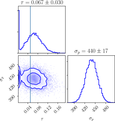
Figure 5: The result of the ensemble test with the two-frequency ILC is shown. The simulated GroundBIRD frequency maps are used. The contours for $1\sigma$ and $2\sigma$ are drawn, and the vertical solid lines in the $\tau$ histogram and contours display the input value of $\tau$. We estimate $\tau$ from the mean and standard deviation of its distribution excluding the peak at the lower boundary. The estimated $\tau$ is 0.067$\pm$0.030 with the total noise level estimate of 440$\pm$17 $\mu\mathrm{K~{}arcmin}$.

We first fit the GroundBIRD maps. The ensemble test is performed with 10 000 samples. For each realization, we remove the foreground first and then estimate $\tau$ from a pixel-based likelihood fit.

The ILC with the two GroundBIRD maps leaves a large foreground residual mainly from the synchrotron component. This residual prevents the correct estimation of $\tau$. To solve this problem, we add a mask to exclude the sky region dominated by large synchrotron residuals from the input map for the likelihood fit. This mask is obtained by applying a threshold to the foreground cleaned map. This extra mask excludes an additional $5\%$ of the sky and enables estimation of the unbiased $\tau$. After applying this mask, the ILC coefficients for 145 and 220 GHz are $c_{145}$=1.470$\pm$0.003 and $c_{220}$=$-$0.470$\pm$0.003, respectively.

The likelihood fit result for the ensemble is shown in Fig. 5, where a contour of $\tau$ versus $\sigma_{p}$ and two histograms of them are shown. The estimated $\tau$ is found to be 0.067$\pm$0.030 when the input $\tau$ is 0.05. The noise level of the foreground cleaned map is found to be 440$\pm$17 $\mu\mathrm{K~{}arcmin}$, to which the white noise and map-making residuals are contributing.

A small peak near the lower boundary of the $\tau$ histogram in Fig. 5 originates from our high noise level. Fluctuation in an ensemble, which simulates the statistical uncertainty of $\tau$, sometimes pushes $\tau$ down to its lower limit that is 0, making such a peak. One way to avoid it is to allow the negative value of $\tau$ in the likelihood. However, since it is not only unclear how to correctly construct the pixel likelihood with the unphysical negative $\tau$ values from the CAMB, but is also not of the main issue of this paper, we limit $\tau$ to non-negative values. We estimate $\tau$ from the mean and standard deviation of its distribution, excluding this peak.

Even after applying the extra mask for the synchrotron, the dominant foreground residual at this stage originates from the synchrotron foreground. We find that the non-zero foreground residuals introduce a bias in $\tau$, which tends to be overestimated by around 10% but is still within $1\sigma$ of the statistical uncertainty.

To remove the synchrotron foreground further, we add the simulated QUIJOTE 30 GHz map as a synchrotron template. The ILC coefficients for the three-frequency case are $c_{145}$=1.485$\pm$0.007, $c_{220}$=$-$0.468$\pm$0.003, and $c_{30}$=$-$0.017$\pm$0.006. The ILC coefficient for 30 GHz ($c_{30}$) is suppressed because the synchrotron foreground dominates over other components at this frequency. Therefore, the synchrotron template removes the synchrotron foreground without significantly changing the map. The estimated $\tau$ is 0.059$\pm$0.029 and the noise level is found to be 440$\pm$17 $\mu\mathrm{K~{}arcmin}$.

Note that the map-making residuals become practically an additional white noise source because their ring patterns are diluted as the maps are degraded to $N_{\mathrm{side}}=8$. We find that the existence of the map-making residuals increases the noise level effectively by 11% and thus the uncertainty of the $\tau$ is increased by around 10%. We discuss the results with and without map-making residuals in Appendix B.

6.2 GroundBIRD and QUIJOTE

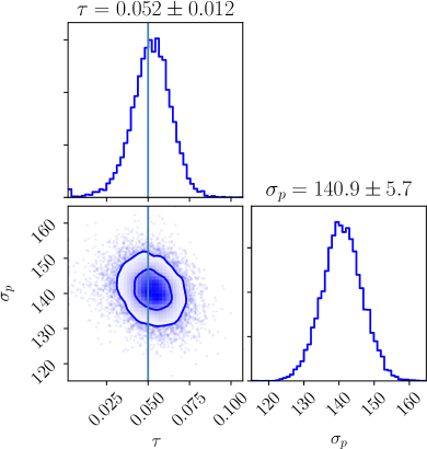
Figure 6: The result of the ensemble test with the eight-frequency ILC is shown. The simulated GroundBIRD maps for {145, 220} GHz and the simulated QUIJOTE maps for {11, 13, 17, 19, 30, 40} GHz are used. The contours for $1\sigma$ and $2\sigma$ are drawn, and the vertical solid lines in the $\tau$ histogram and the contour plot display the input value of $\tau$. The estimated $\tau$ is 0.052$\pm$0.012.

We estimate $\tau$ again by including the simulated QUIJOTE frequency maps at 11, 13, 17, 19, 30, and 40 GHz in our analysis. We generate the foreground and noise maps for QUIJOTE in a similar way as for the GroundBIRD maps. Here the $1/f$ noise component is not included in the QUIJOTE maps and is a potential limitation of our analysis. We discuss this point in the following section. The pixel noise levels of the polarization maps and the resulting ILC coefficients are summarized in Table 2. In this case, the map-making residuals are included only in the GroundBIRD maps, and the ILC coefficients of the GroundBIRD maps are relatively smaller than in previous cases. The effect of the map-making residuals, therefore, becomes small.

Table 2: Noise levels of polarization maps and ILC coefficients for the eight-frequency result are summarized. The constraint of $\sum_{\nu}c_{\nu}=1$ is numerically incorrect due to the rounding off of fit results.

Frequency	Noise level	ILC coefficients
(GHz)	($\mu\mathrm{K~{}arcmin}$)
11	3600	$-$0.011$\pm$	0.001
13	3600	$-$0.009$\pm$	0.002
17	5100	$-$0.003$\pm$	0.002
19	5100	$-$0.002$\pm$	0.002
30	160	$-$0.14$\pm$	0.04
40	91	1.12$\pm$	0.04
145	110	0.13$\pm$	0.03
220	780	$-$0.077$\pm$	0.008

The result of the eight-frequency case is shown in Fig. 6. The estimated $\tau$ is found to be 0.052$\pm$0.012 with the total noise level of 141$\pm$6 $\mu\mathrm{K~{}arcmin}$. The noise level is reduced by 70% compared to the three-frequency result because the contribution of the 220 GHz map with a high noise level is suppressed dominantly by adding 30 and 40 GHz maps. Accordingly, the sensitivity on the $\tau$ is improved compared to the three-frequency case.

6.3 Limitations of current analysis

We include several sources of systematic errors for realistic simulations: atmospheric noise, detector calibration, and map-making residuals. However, there are potential sources of systematic error that are not included in this study.

We assume that our fast-scanning technique, in combination with the sparse wire-grid calibration removes most of the atmospheric noise. Therefore, we do not consider the effect of frequency-dependent atmospheric fluctuations (Lay & Halverson, 2000) in this work. The systematic effects from the optical system are incomplete. For example, the uncertainty of the polarization angle and imperfect focusing due to the aberration of the reflectors are not included in our analysis. The detailed study for the sidelobes and spillover patterns is also in progress.

In our TOD simulation, we do not consider the systematic effects due to data cuts, potential pointing offsets and detector gain variations. These should be addressed when analyzing the real observations.

As is mentioned earlier, the foreground and noise maps for QUIJOTE do not contain the $1/f$ noise, since the behavior of $1/f$ noise for QUIJOTE is not available to us at this stage. Once this information is available, we plan to include it in our analysis. We will address all the issues discussed here in a future publication.

7 Conclusions

We have performed estimates of the optical depth to reionization ($\tau$) with simulated data for the GroundBIRD experiment. We started the simulation from TOD with the inclusion of $1/f$ noise in our simulation. The input maps cover 45% of the sky (22.8% after masking the Galactic plane). These maps included the CMB realization, foregrounds, expected noise, and map-making residuals. We assumed a three-year observation with 161 detectors in total. We cleaned the polarization foregrounds using the ILC method, which requires at least three frequency maps to remove two foreground components; namely, synchrotron and dust foregrounds. We also added the simulated QUIJOTE maps for better foreground cleaning. To estimate the $\tau$ values, we used our pixel-based likelihood.

The estimated $\tau$ is 0.067$\pm$0.030 with GroundBIRD maps only and 0.059$\pm$0.029 with a synchrotron template included, where the input value is 0.05. Adding QUIJOTE frequency maps to the GroundBIRD maps further removed the foregrounds and reduced the noise level. The estimated $\tau$ with eight-frequency (11, 13, 17, 19, 30, 40, 145, and 220 GHz) ILC is found to be 0.052$\pm$0.012. The incomplete foreground cleaning tends to introduce additional bias into the $\tau$ estimate. The uncertainty in the $\tau$ estimate is constrained mainly by the pixel noise level of the foreground cleaned map. The map-making residuals increase the noise level and degrade the sensitivity to $\tau$. In our case, $\tau$ sensitivity is degraded by about 10%, which depends on the observing strategy and detector set-up.

Appendix A Estimation of noise equivalent temperature of GroundBIRD

We estimate our noise level by considering the KID response, the optical efficiency, and the atmospheric emission. The noise equivalent power (NEP) is given by (Zmuidzinas, 2012; Flanigan et al., 2016)

$$\mathrm{NEP}^{2}=\frac{1}{\eta_{\mathrm{opt}}}\int d\nu\left[2h\nu P_{\mathrm{rad}}(\nu)\left\{1+\eta_{\mathrm{opt}}\eta_{\mathrm{em}}(\nu)\bar{n}_{\mathrm{bb}}F(\nu)\right\}+\frac{4\Delta}{\eta_{\mathrm{pb}}}P_{\mathrm{rad}}(\nu)\right]$$ (A1)

where $h$ is the Planck constant, $\nu$ is the frequency of the incoming radiation, $P_{\mathrm{rad}}(\nu)$ is the radiation power density in $\mathrm{pW/\sqrt{Hz}}$, reaching the telescope window at a given elevation angle, and $\eta_{\mathrm{em}}(\nu)$ is the sky emissivity that depends on the frequency. To compute $P_{\mathrm{rad}}(\nu)$ and $\eta_{\mathrm{em}}(\nu)$, we use the atmospheric antenna temperature for airmass of $1/\sin(70^{\arcdeg})$ derived from the atmospheric transmission at microwave model (Pardo et al., 2001), which is evaluated assuming average conditions at the Teide observatory (pressure of 770.0 mbar and precipitable water vapor (PWV) of 3.5 mm (Castro-Almazán et al., 2016)). For the actual modeling, we assume the PWV value to be 4.0 mm.

The $\eta_{\mathrm{opt}}$ is the net optical efficiency of our optical system, $\bar{n}_{\mathrm{bb}}$ is the mean photon number emitted from blackbody, $\eta_{\mathrm{pb}}$ is the Cooper-pair breaking efficiency, and $F(\nu)$ is the total transmissivity of the filters that are used in GroundBIRD optics. The $\Delta$ is the gap energy of the superconducting material which is given by $1.76k_{B}T_{c}$ where $k_{B}$ is the Boltzmann constant and $T_{c}$ is the superconducting transition temperature ($T_{c}=1.28\ \mathrm{K}$ for the aluminum thin film (Kutsuma et al., 2020)). The NEP calculation assumes the atmosphere to be a blackbody source. The parameters and their values used for this estimation are summarized in Table 3. The frequency-dependent parameters are shown by nominal values in our frequency bands, and the radiation power ($\mathcal{P}_{\mathrm{rad}}$) is integrated over our frequency band with a width of 60 GHz, for both 145 and 220 GHz. The estimated NEP are $160\ \mathrm{aW\sqrt{s}}$ and $290\ \mathrm{aW\sqrt{s}}$ for 145 GHz and 220 GHz, respectively. The corresponding NET values in CMB temperature are $820\ \mu\mathrm{K~{}\sqrt{s}}$ and $2600\ \mu\mathrm{K~{}\sqrt{s}}$ for 145 GHz and 220 GHz, respectively.

Parameter	145 GHz	220 GHz
$\mathcal{P}_{\mathrm{rad}}$ [$\mathrm{pW}$]	13	28
$F(\nu)$	0.5	0.5
$\eta_{\mathrm{em}}(\nu)$	0.15	0.28
$\eta_{\mathrm{opt}}$	0.38	0.30
$\eta_{\mathrm{pb}}$	0.4	0.4
$\bar{n}_{\mathrm{bb}}$	38.7	25.4

Table 3: The parameters and their nominal values at two frequency bands used for the estimation of NEP of the GroundBIRD detectors are summarized.

Appendix B Likelihood fit results for other set-ups

In this section, we summarize the results of ensemble tests for several foreground set-ups. The estimates of $\tau$ and total noise level $\sigma_{p}$ are summarized in Table 4. The simplest case is the “No foregrounds” case, where it is assumed that the foreground is cleaned completely. The input map contains CMB and noise only, and the same noise level as the “Two-frequency ILC” case is assumed. The estimated $\tau$ is 0.060$\pm$0.029 when the input value is 0.05, with an estimate of the white noise level of 397$\pm$17 $\mu\mathrm{K~{}arcmin}$. This uncertainty is 7% greater than the estimate by Fisher matrix, $\sigma_{\tau}$= 0.027, with the same noise input. The estimated $\tau$ has a large bias ($\sim 0.01$) from the input value but it is still within the uncertainty. We test this case with smaller noise levels and find that a large noise tends to make a positive bias in $\tau$ estimation.

The cases with ILC are tested in two ways: with and without map-making residuals. For the two-frequency case, the estimated $\tau$ is 0.066$\pm$0.028, and $\sigma_{p}$ is 395$\pm$16 $\mu\mathrm{K~{}arcmin}$ without the map-making residuals. With the map-making residuals, the estimated $\tau$ is 0.067$\pm$0.030, and $\sigma_{p}$ is 440$\pm$17 $\mu\mathrm{K~{}arcmin}$. The map-making residuals increase the noise level by 10% and also increase the $\tau$ uncertainty by around 10%. As discussed in section 6.1, incomplete foreground cleaning with two frequency maps tends to create an additional bias of around 10% in $\tau$ estimate.

In the three-frequency cases, we expect the synchrotron to be removed effectively by adding a 30 GHz map. Without the map-making residuals, the estimated $\tau$ is 0.056$\pm$0.026, with the estimated noise level of 394$\pm$15 $\mu\mathrm{K~{}arcmin}$. The $\tau$ uncertainty and the white noise level are at almost same level as the two-frequency map case. Adding a synchrotron template map at 30 GHz cleans the synchrotron foreground better, so the estimated $\tau$ is closer to the input value. With the map-making residuals, the estimated $\tau$ is 0.059$\pm$0.029 which has about 10% larger uncertainty compared to the value without map-making residuals. The noise level is almost same with the two-frequency case.

The eight-frequency map case uses all six QUIJOTE frequency maps with the GroundBIRD frequency maps. The map-making residuals are included only for the GroundBIRD frequency maps because we are not doing map-making for the QUIJOTE maps. The estimated value of $\tau$ is 0.052$\pm$0.012 and noise level is 139$\pm$6 $\mu\mathrm{K~{}arcmin}$ without the map-making residuals and $\tau$ is 0.052$\pm$0.012 and noise level is 141$\pm$6 $\mu\mathrm{K~{}arcmin}$ with the map-making residuals. Since the noise levels are smaller than the two or three-frequency cases, the bias in $\tau$ is suppressed. In this case, the map-making residuals slightly increase the noise level, but have a negligible effect on the estimation of $\tau$ because the contribution of the GroundBIRD 220 GHz map, which has a large white noise level and the map-making residuals, becomes small by adding the QUIJOTE maps.

Table 4: The estimates of $\tau$ and the pixel noise level of the combined map $\sigma_{p}$ for different foreground cleaning methods are summarized. For the “Fisher matrix” case, the same noise level as the two-frequency map case is assumed and the $\tau$ uncertainty is estimated from the Fisher matrix approach. Other estimates are from the pixel-based likelihood approach. The “No foregrounds” is the case with an input map combining only the CMB and noise. The same noise with “Two-frequency ILC” case is assumed. The “Two-frequency ILC” is the case performing the foreground cleaning with only two frequency maps of GroundBIRD. For the “Three-frequency ILC” case, a 30 GHz map is added to the two-frequency case, as a synchrotron template. The“Eight-frequency ILC” is the case with eight frequency maps, including all the QUIJOTE frequency maps. The cases with foregrounds are tested with and without the map-making residuals.

Foreground cleaning method	$\tau$		$\sigma_{p}\ (\mu\mathrm{K~{}arcmin})$
Fisher matrix	0.050$\pm$	0.027	395
No foregrounds	0.060$\pm$	0.029	397	$\pm$17
Two-frequency ILC	0.066$\pm$	0.028	395	$\pm$16
Two-frequency ILC with map-making residuals	0.067$\pm$	0.030	440	$\pm$17
Three-frequency ILC	0.056$\pm$	0.026	394	$\pm$15
Three-frequency ILC with map-making residuals	0.059$\pm$	0.029	440	$\pm$17
Eight-frequency ILC	0.052$\pm$	0.012	139	$\pm$ 6
Eight-frequency ILC with map-making residuals	0.052$\pm$	0.012	141	$\pm$ 6

References

- Ade et al. (2019) Ade, P., Aguirre, J., Ahmed, Z., et al. 2019, Journal of Cosmology and Astroparticle Physics, 2019, 056, doi: 10.1088/1475-7516/2019/02/056
- Albrecht & Steinhardt (1982) Albrecht, A., & Steinhardt, P. J. 1982, Phys. Rev. Lett., 48, 1220, doi: 10.1103/PhysRevLett.48.1220
- Allison et al. (2015) Allison, R., Caucal, P., Calabrese, E., Dunkley, J., & Louis, T. 2015, Phys. Rev. D, 92, 123535, doi: 10.1103/PhysRevD.92.123535
- Astropy Collaboration et al. (2013) Astropy Collaboration, Robitaille, T. P., Tollerud, E. J., et al. 2013, A&A, 558, A33, doi: 10.1051/0004-6361/201322068
- Astropy Collaboration et al. (2018) Astropy Collaboration, Price-Whelan, A. M., SipHocz, B. M., et al. 2018, aj, 156, 123, doi: 10.3847/1538-3881/aabc4f
- Bryan et al. (2018) Bryan, S., Ade, P., Bond, J. R., et al. 2018, Journal of Low Temperature Physics, 193, 1033, doi: 10.1007/s10909-018-2031-z
- Castro-Almazán et al. (2016) Castro-Almazán, J. A., Muñoz-Tuñón, C., García-Lorenzo, B., et al. 2016, in Observatory Operations: Strategies, Processes, and Systems VI, ed. A. B. Peck, R. L. Seaman, & C. R. Benn, Vol. 9910, International Society for Optics and Photonics (SPIE), 227 – 236, doi: 10.1117/12.2232646
- Chon et al. (2004) Chon, G., Challinor, A., Prunet, S., Hivon, E., & Szapudi, I. 2004, MNRAS, 350, 914, doi: 10.1111/j.1365-2966.2004.07737.x
- Day et al. (2003) Day, P. K., LeDuc, H. G., Mazin, B. A., Vayonakis, A., & Zmuidzinas, J. 2003, Nature, 425, 817, doi: 10.1038/nature02037
- Eriksen et al. (2004) Eriksen, H. K., Banday, A. J., Gorski, K. M., & Lilje, P. B. 2004, The Astrophysical Journal, 612, 633, doi: 10.1086/422807
- Ferraro & Smith (2018) Ferraro, S., & Smith, K. M. 2018, Phys. Rev. D, 98, 123519, doi: 10.1103/PhysRevD.98.123519
- Flanigan et al. (2016) Flanigan, D., McCarrick, H., Jones, G., et al. 2016, Applied Physics Letters, 108, 083504, doi: 10.1063/1.4942804
- Foreman-Mackey (2016) Foreman-Mackey, D. 2016, The Journal of Open Source Software, 1, 24, doi: 10.21105/joss.00024
- Franceschet et al. (2018) Franceschet, C., Realini, S., Mennella, A., et al. 2018, in Millimeter, Submillimeter, and Far-Infrared Detectors and Instrumentation for Astronomy IX, ed. J. Zmuidzinas & J.-R. Gao, Vol. 10708, International Society for Optics and Photonics (SPIE), 170 – 186, doi: 10.1117/12.2313558
- Génova-Santos et al. (2015) Génova-Santos, R., Rubiño Martín, J. A., Rebolo, R., et al. 2015, Highlights of Spanish Astrophysics VIII
- Górski et al. (2005) Górski, K. M., Hivon, E., Banday, A. J., et al. 2005, ApJ, 622, 759, doi: 10.1086/427976
- Goupy et al. (2016) Goupy, J., Adane, A., Benoit, A., et al. 2016, Journal of Low Temperature Physics, 184, 661, doi: 10.1007/s10909-016-1531-y
- Guth (1981) Guth, A. H. 1981, Phys. Rev. D, 23, 347, doi: 10.1103/PhysRevD.23.347
- Génova-Santos et al. (2015) Génova-Santos, R., Rubiño-Martín, J. A., Rebolo, R., et al. 2015, Monthly Notices of the Royal Astronomical Society, 452, 4169, doi: 10.1093/mnras/stv1405
- Honda et al. (2020) Honda, S., Choi, J., Génova-Santos, R. T., et al. 2020, in Ground-based and Airborne Telescopes VIII, ed. H. K. Marshall, J. Spyromilio, & T. Usuda, Vol. 11445, International Society for Optics and Photonics (SPIE), 1379 – 1386, doi: 10.1117/12.2560918
- Hu & White (1997) Hu, W., & White, M. 1997, Phys. Rev. D, 56, 596, doi: 10.1103/PhysRevD.56.596
- iminuit team (2018) iminuit team. 2018, iminuit – A Python interface to Minuit, https://github.com/scikit-hep/iminuit
- Kamionkowski et al. (1997a) Kamionkowski, M., Kosowsky, A., & Stebbins, A. 1997a, Phys. Rev. Lett., 78, 2058, doi: 10.1103/PhysRevLett.78.2058
- Kamionkowski et al. (1997b) —. 1997b, Phys. Rev. D, 55, 7368, doi: 10.1103/PhysRevD.55.7368
- Keihänen et al. (2010) Keihänen, E., Keskitalo, R., Kurki-Suonio, H., Poutanen, T., & Sirviö, A.-S. 2010, A&A, 510, A57, doi: 10.1051/0004-6361/200912813
- Keihänen et al. (2005) Keihänen, E., Kurki-Suonio, H., & Poutanen, T. 2005, Monthly Notices of the Royal Astronomical Society, 360, 390, doi: 10.1111/j.1365-2966.2005.09055.x
- Kermish et al. (2012) Kermish, Z., et al. 2012, Proc. SPIE Int. Soc. Opt. Eng., 8452, 1C, doi: 10.1117/12.926354
- Kutsuma et al. (2020) Kutsuma, H., Sueno, Y., Hattori, M., et al. 2020, AIP Advances, 10, 095320, doi: 10.1063/5.0013946
- Lay & Halverson (2000) Lay, O. P., & Halverson, N. W. 2000, The Astrophysical Journal, 543, 787, doi: 10.1086/317115
- Ledoit & Wolf (2004) Ledoit, O., & Wolf, M. 2004, Journal of Multivariate Analysis, 88, 365, doi: 10.1016/S0047-259X(03)00096-4
- Lee et al. (2008) Lee, A. T., Tran, H., Ade, P., et al. 2008, AIP Conference Proceedings, 1040, 66, doi: 10.1063/1.2981555
- Lewis et al. (2000) Lewis, A., Challinor, A., & Lasenby, A. 2000, ApJ, 538, 473, doi: 10.1086/309179
- Linde (1982) Linde, A. 1982, Physics Letters B, 116, 335 , doi: https://doi.org/10.1016/0370-2693(82)90293-3
- McMahon et al. (2009) McMahon, J. J., Aird, K. A., Benson, B. A., et al. 2009, AIP Conference Proceedings, 1185, 511, doi: 10.1063/1.3292391
- Ogburn IV et al. (2012) Ogburn IV, R. W., Ade, P. A. R., Aikin, R. W., et al. 2012, in Millimeter, Submillimeter, and Far-Infrared Detectors and Instrumentation for Astronomy VI, ed. W. S. Holland, Vol. 8452, International Society for Optics and Photonics (SPIE), 340 – 353, doi: 10.1117/12.925731
- Pardo et al. (2001) Pardo, J., Cernicharo, J., & Serabyn, E. 2001, IEEE Transactions on Antennas and Propagation, 49, 1683, doi: 10.1109/8.982447
- Planck Collaboration (2016) Planck Collaboration. 2016, Astronomy & Astrophysics, 594, A11, doi: 10.1051/0004-6361/201526926
- Planck Collaboration (2020) —. 2020, Astronomy & Astrophysics, 641, A6, doi: 10.1051/0004-6361/201833910
- Python Core Team (2015) Python Core Team. 2015, Python: A dynamic, open source programming language. https://www.python.org/
- Rubiño-Martín et al. (2012) Rubiño-Martín, J. A., Rebolo, R., Aguiar, M., et al. 2012, in Ground-based and Airborne Telescopes IV, ed. L. M. Stepp, R. Gilmozzi, & H. J. Hall, Vol. 8444, International Society for Optics and Photonics (SPIE), 987 – 997, doi: 10.1117/12.926581
- Sato (1981) Sato, K. 1981, Monthly Notices of the Royal Astronomical Society, 195, 467, doi: 10.1093/mnras/195.3.467
- Seljak & Zaldarriaga (1997) Seljak, U. b. u., & Zaldarriaga, M. 1997, Phys. Rev. Lett., 78, 2054, doi: 10.1103/PhysRevLett.78.2054
- Smith & Zaldarriaga (2007) Smith, K. M., & Zaldarriaga, M. 2007, Physical Review D, 76, 043001, doi: 10.1103/PhysRevD.76.043001
- Starobinsky (1980) Starobinsky, A. 1980, Physics Letters B, 91, 99, doi: https://doi.org/10.1016/0370-2693(80)90670-X
- Stebor et al. (2016) Stebor, N., Ade, P., Akiba, Y., et al. 2016, in Proc. SPIE 9914, Millimeter, Submillimeter, and Far-Infrared Detectors and Instrumentation for Astronomy VIII, 99141H, 99141H, doi: 10.1117/12.2233103
- Swetz et al. (2011) Swetz, D. S., Ade, P. A. R., Amiri, M., et al. 2011, The Astrophysical Journal Supplement Series, 194, 41, doi: 10.1088/0067-0049/194/2/41
- Tajima et al. (2012) Tajima, O., Choi, J., Hazumi, M., et al. 2012, in Millimeter, Submillimeter, and Far-Infrared Detectors and Instrumentation for Astronomy VI, ed. W. S. Holland, Vol. 8452, International Society for Optics and Photonics (SPIE), 468 – 476, doi: 10.1117/12.925816
- Tegmark & Oliveria-Costa (2001) Tegmark, M., & Oliveria-Costa, A. d. 2001, Physical Review D, 64, 063001, doi: 10.1103/PhysRevD.64.063001
- Thorne et al. (2017) Thorne, B., Dunkley, J., Alonso, D., & Næss, S. 2017, Monthly Notices of the Royal Astronomical Society, 469, 2821, doi: 10.1093/mnras/stx949
- Watts et al. (2018) Watts, D. J., Wang, B., Ali, A., et al. 2018, The Astrophysical Journal, 863, 121, doi: 10.3847/1538-4357/aad283
- Won (2018) Won, E. 2018, EPJ Web Conf., 168, 01014, doi: 10.1051/epjconf/201816801014
- Wu et al. (2014) Wu, W. L. K., Errard, J., Dvorkin, C., et al. 2014, The Astrophysical Journal, 788, 138, doi: 10.1088/0004-637x/788/2/138
- Zaldarriaga (1997) Zaldarriaga, M. 1997, Phys. Rev. D, 55, 1822, doi: 10.1103/PhysRevD.55.1822
- Zaldarriaga (1998) —. 1998, The Astrophysical Journal, 503, 1, doi: 10.1086/305987
- Zaldarriaga & Seljak (1997) Zaldarriaga, M., & Seljak, U. c. v. 1997, Phys. Rev. D, 55, 1830, doi: 10.1103/PhysRevD.55.1830
- Zmuidzinas (2012) Zmuidzinas, J. 2012, Annual Review of Condensed Matter Physics, 3, 169, doi: 10.1146/annurev-conmatphys-020911-125022
- Zonca et al. (2019) Zonca, A., Singer, L., Lenz, D., et al. 2019, Journal of Open Source Software, 4, 1298, doi: 10.21105/joss.01298