Bias-Variance Reduced Local SGD for Less Heterogeneous Federated Learning

Abstract

Recently, local SGD has got much attention and been extensively studied in the distributed learning community to overcome the communication bottleneck problem. However, the superiority of local SGD to minibatch SGD only holds in quite limited situations. In this paper, we study a new local algorithm called Bias-Variance Reduced Local SGD (BVR-L-SGD) for nonconvex distributed optimization. Algorithmically, our proposed bias and variance reduced local gradient estimator fully utilizes small second-order heterogeneity of local objectives and suggests randomly picking up one of the local models instead of taking the average of them when workers are synchronized. Theoretically, under small heterogeneity of local objectives, we show that BVR-L-SGD achieves better communication complexity than both the previous non-local and local methods under mild conditions, and particularly BVR-L-SGD is the first method that breaks the barrier of communication complexity $\Theta(1/\varepsilon)$ for general nonconvex smooth objectives when the heterogeneity is small and the local computation budget is large. Numerical results are given to verify the theoretical findings and give empirical evidence of the superiority of our method.

1 Introduction

Nowadays, optimization problems arising in machine learning are often large and require huge computational time. Distributed learning is one of the attractive approaches to reduce the computational time by utilizing parallel computing. In classical distributed learning, each worker has the whole dataset used in optimization or a random subset of the whole dataset which is not explicitly exchanged. In recent federated learning, introduced by Konečnỳ et al. (2015); Shokri & Shmatikov (2015); McMahan et al. (2017), we build a global model across multiple devices or servers without explicitly exchanging their own local datasets, and local datasets can be heterogeneous, i.e., each local dataset may be generated from a different distribution. There are various federated learning scenarios (e.g., personalization, preservation of the privacy of local information, robustness to attacks and failures, guarantees of fairness) and refer to the extensive survey (Kairouz et al., 2019) for these topics.

One of the most naive and widely used approaches to distributed learning is minibatch Stochastic Gradient Descent (SGD) (Dekel et al., 2012), which is also called as Federated Averaging (FedAvg) (McMahan et al., 2017). Each worker computes minibatch stochastic gradient of the own local objective and then their average is used to update the global model. Also, more computationally efficient methods including minibatch Stochastic Variance Reduced Gradient (SVRG) (Johnson & Zhang, 2013; Allen-Zhu & Hazan, 2016; Reddi et al., 2016a) and its variant (Lei et al., 2017), minibatch StochAstic Recursive grAdient algoritHm (SARAH) (Nguyen et al., 2017, 2019) and its variants (Fang et al., 2018; Zhou et al., 2018) are applicable to the problem. Particularly, SARAH achieves the optimal total computational complexity in nonconvex optimization.

Unfortunately, minibatch methods suffer from their communication cost because of the necessity to communicate local gradients for every single global update. One of the possible solutions is using a large batch to compute local gradients (Goyal et al., 2017), but the communication complexity, that is the necessary number of communication rounds to optimize, is theoretically never smaller than the one of deterministic GD and thus communication cost is still problematic.

To overcome the communication bottleneck problem, local methods have got much attention due to its empirical effectiveness (Konečnỳ et al., 2015; Lin et al., 2018). In local SGD (also called Parallel Restart SGD), each worker independently updates the local model based on his own local dataset, and periodically communicates and averages the local models. Many papers (Stich, 2018; Yu et al., 2019; Haddadpour & Mahdavi, 2019; Haddadpour et al., 2019; Koloskova et al., 2020; Khaled et al., 2020) have stated the superiority of local SGD to minibatch SGD, but these results are based on unfair comparisons and hence not satisfactory. Concretely, they have compared the two algorithms with the same local minibatch size $b$, which means that local SGD with $K$ local updates requires $K$ times larger number of local computations per communication round than minibatch SGD. If we fix the number of single stochastic gradient computations per communication round to $\mathcal{B}:=Kb$ for each worker, their results indicates that the communication complexity of local SGD with $K$ local updates and $b$ local minibatch size are never better than the one of minibatch SGD with $\mathcal{B}$ local minibatch size for any $\mathcal{B}$. This point is quite important, but many papers have overlooked it.

Recently, Woodworth et al. (2020b, a) have shown that, for the first time, theoretical superiority of local SGD to minibatch SGD under fair comparison for convex optimization when the heterogeneity of local objectives is small. On the other hand, their derived lower bound of local SGD also suggests the limitation of local SGD. Specifically, they have shown that if the first-order heterogeneity of local objectives is greater than $\sqrt{\varepsilon}$, where $\varepsilon$ is the desired optimization accuracy, the communication complexity of local SGD is even worse than the one of minibatch SGD. In other words, the quite small heterogeneity of local objectives is essential for the superiority of local SGD to minibatch SGD, which is a clear limitation of local SGD. SCAFFOLD (Karimireddy et al., 2020b) is a new local algorithm based on the idea of reducing their called client-drift, which uses a similar formulation to the variance reduction technique. However, the communication complexity is the same as minibatch SGD for general nonconvex objectives and it requires small heterogeneity and quadraticity of local objectives to surpass minibatch SGD, which is also quite limited. Inexact DANE (Reddi et al., 2016b) is another variant of local methods that uses a general local subsolver that returns an approximate minimizer of the regularized local objective. Again, the superiority to non-local methods has been only shown for quadratic convex objectives.

In summary, both in classical distributed learning and recent federated learning, naive minibatch (i.e., non-local) methods often suffer from their communication cost. Several local methods surpass non-local ones in terms of communication complexity. However, the necessary conditions for the superiority of the previous local algorithms to non-local ones are quite limited (i.e., extremely small heterogeneity or quadraticity of local objectives). A natural question is that: is there a local algorithm which surpasses non-local (and existing local) ones in terms of communication complexity with a fixed local computation budget under more relaxed conditions?

Algorithm	Communication Complexity	Extra Assumptions
Minibatch SGD	$\frac{1}{\varepsilon}+\frac{1}{\mathcal{B}P\varepsilon^{2}}$	None
Minibatch SARAH (Nguyen et al., 2019)	$\frac{1}{\varepsilon}+\frac{\sqrt{n\wedge\frac{1}{\varepsilon}}}{\mathcal{B}P\varepsilon}$	None
Local SGD (Yu et al., 2019)	$\frac{1}{\mathcal{B}\varepsilon}+\frac{1}{\mathcal{B}P\varepsilon^{2}}+\frac{1}{\varepsilon^{\frac{3}{2}}}$	$G$ gradient boundedness
Local SGD (Khaled et al., 2020)	$\frac{1+\sigma_{\mathrm{dif}}^{4}}{\mathcal{B}P\varepsilon^{2}}+\frac{\sigma_{\mathrm{dif}}^{2}\mathcal{B}P}{\varepsilon}$	convexity $\mathcal{B}\leq\frac{1+\sigma_{\mathrm{dif}}^{2}}{P\varepsilon}$ or $\sigma_{\mathrm{dif}}^{2}\geq\varepsilon$
Local SGD (Woodworth et al., 2020a)	$\frac{1}{\mathcal{B}\varepsilon}+\frac{1}{\mathcal{B}P\varepsilon^{2}}+\frac{1}{\sqrt{\mathcal{B}}\varepsilon^{\frac{3}{2}}}+\frac{\zeta_{1}}{\varepsilon^{\frac{3}{2}}}$	convexity, $1$st-order $\zeta_{1}$ heterogeneity
Local SGD (Woodworth et al., 2020a) (Lower bound)	$\frac{1}{\mathcal{B}\varepsilon^{\frac{3}{2}}}+\frac{1}{\mathcal{B}P\varepsilon^{2}}+\left(\frac{1}{\varepsilon}\wedge\frac{\zeta_{1}}{\varepsilon^{\frac{3}{2}}}\right)$	convexity, $1$st-order $\zeta_{1}$ heterogeneity
SCAFFOLD (Karimireddy et al., 2020b)	$\frac{1}{\varepsilon}+\frac{1}{\mathcal{B}P\varepsilon^{2}}$	None
SCAFFOLD (Karimireddy et al., 2020b)	$\frac{1}{\mathcal{B}\varepsilon}+\frac{1}{\mathcal{B}P\varepsilon^{2}}+\frac{\zeta}{\varepsilon}$	quadraticity, $2$nd-order $\zeta$ heterogeneity
BVR-L-SGD (this paper)	$\frac{1}{\sqrt{\mathcal{B}}\varepsilon}+\frac{\sqrt{n\wedge\frac{1}{\varepsilon}}}{\mathcal{B}P\varepsilon}+\frac{\zeta}{\varepsilon}$	$2$nd-order $\zeta$ heterogeneity

Table 1: Comparison of the order of the necessary number of communication rounds to satisfy $\mathbb{E}\|f(x_{\mathrm{out}})\|^{2}\leq\varepsilon$ (or $f(x_{\mathrm{out}})-f(x_{*})\leq\varepsilon$ for convex $f$). "Extra Assumptions” indicates the necessary assumptions to derive the results other than Assumptions 2, 3 and 4 in Section 2. $\varepsilon$ is the desired optimization accuracy. $\mathcal{B}$ is the local computation budget that is the allowed number of single stochastic gradient computations per communication round for each worker. $P$ is the number of workers. $n$ is the total number of samples and is possibly $\infty$ in online (i.e., expected risk minimization) settings. The smoothness of local objectives $L$, the variance of a single stochastic gradient $\sigma^{2}$ and gradient boundedness $G$ are regarded as $\Theta(1)$ for ease of presentation. Note that in this notation, second-order heterogeneity $\zeta$ always satisfies $\zeta\leq\Theta(L)=\Theta(1)$. $\sigma_{\mathrm{dif}}^{2}$ is the squared local gradient norm at an optimum (for the precise definition, see (Khaled et al., 2020)).

Main Contributions

We propose a new local algorithm called Bias-Variance Reduced Local SGD (BVR-L-SGD) for nonconvex distributed learning. The main features of our method are as below.

Algorithmic Features. The algorithm is based on our bias and variance reduced gradient estimator that simultaneously reduces the bias caused by local updates and the variance caused by stochastization based on the idea of SARAH like variance reduction technique. Importantly, to fully utilize the second-order heterogeneity of local objectives, a randomly picked local model is used as a synchronized global model instead of taking the average of them, which is typical in the previous local methods.

Theoretical Features. We analyse BVR-L-SGD for general nonconvex smooth objectives under second-order heterogeneity assumption, which interpolates the heterogeneity of local objectives between the identical case and the extremely non-IID case, and plays a critical role in our nonconvex analysis. The comparison of the communication complexities of our method with the most relevant existing results is given in Table 1. The communication complexity of BVR-L-SGD has a better dependence on $\varepsilon$ than minibatch SGD, local SGD and SCAFFOLD. When $\mathcal{B}P\gg\sqrt{n\wedge 1/\varepsilon}$ and the second-order heterogeneity $\zeta$ of local objectives is small relative to the smoothness $L$, BVR-L-SGD strictly surpasses minibatch SARAH. Furthermore, BVR-L-SGD is the first method that breaks the barrier of communication complexity $1/\varepsilon$ when local computation budget $\mathcal{B}\to\infty$, for general smooth nonconvex objectives with small heterogeneity $\zeta$. Importantly, even when the heterogeneity is high, the communication complexity of our method is never worse than the ones of the existing methods since the second-order heterogeneity $\zeta$ is bounded by two times the smoothness $L$ of local objectives.

As a result, BVR-L-SGD is a novel and promising communication efficient method for nonconvex optimization both in classical distributed learning (i.e., local data distributions are nearly identical) and recent federated learning (i.e., local data distributions can be highly heterogeneous).

Other Related Work. Several recent papers have also studied local algorithms combined with variance reduction technique (Sharma et al., 2019; Das et al., 2020; Karimireddy et al., 2020a). Sharma et al. (2019) have considered Parallel Restart SPIDER (PR-SPIDER), that is a local variant of SPIDER (Fang et al., 2018) and shown that the proposed algorithm achieves the optimal total computational complexity and the communication complexity of $1/\varepsilon$ for noncovnex smooth objectives. However, these rates essentially match the ones of non-local SARAH and no advantage of localization has been shown. Also, Das et al. (2020) have considered a SPIDER like local algorithm called FedGLOMO but the derived communication complexity is only $1/\varepsilon^{3/2}$ in general and the rate is even worse than minibatch SARAH. Karimireddy et al. (2020a) have proposed MIME, which is essentially a combination of local SGD and SVRG-like variance reduction technique. They have shown that MIME achieves the communication complexity of $1/(\mathcal{B}\varepsilon)+1/(P^{3/4}\varepsilon^{3/2})+\zeta/\varepsilon$ for $\zeta$ second-order heterogeneous nonconvex smooth objectives. Importantly, the second term of the rate of BVR-L-SGD has better dependencies on $P$ and $\mathcal{B}$ than the one of MIME. Particularly, BVR-L-SGD achieves $\zeta/\varepsilon$ when $\mathcal{B}\to\infty$ but MIME does not possess this property.

2 Problem Definition and Assumptions

In this section, we first introduce the notations used in this paper. Then, the problem setting considered in this paper is illustrated and theoretical assumptions are given.

Notation. $\|\cdot\|$ denotes the Euclidean $L_{2}$ norm $\|\cdot\|_{2}$: $\|x\|=\sqrt{\sum_{i}x_{i}^{2}}$ for vector $x$. For a matrix $X$, $\|X\|$ denotes the induced norm by the Euclidean $L_{2}$ norm. For a natural number $m$, $[m]$ denotes the set $\{1,2,\ldots,m\}$. For a set $A$, $\#A$ means the number of elements, which is possibly $\infty$. For any number $a,b$, $a\vee b$ and $a\wedge b$ denote $\mathrm{max}\{a,b\}$ and $\mathrm{min}\{a,b\}$ respectively. We denote the uniform distribution over $A$ by $\mathrm{Unif}(A)$.

2.1 Problem Setting

We want to minimize nonconvex smooth objective

$$f(x):=\frac{1}{P}\sum_{p=1}^{P}f_{p}(x),\text{ where }f_{p}(x):=\mathbb{E}_{z\sim D_{p}}[\ell(x,z)]$$

for $x\in\mathbb{R}^{d}$, where $D_{p}$ is the data distribution associated with worker $p$. Although we consider both offline (i.e., $\#\mathrm{supp}(D_{p})<\infty$ for every $p\in[P]$) and online (i.e., $\#\mathrm{supp}(D_{p})=\infty$ for some $p\in[P]$) settings, it is assumed for offline settings that each local dataset has an equal number of samples, i.e., $\#\mathrm{supp}(D_{p})=\#\mathrm{supp}(D_{p^{\prime}})$ for every $p,p^{\prime}\in[P]$ just for simplicity. We assume that each worker $p$ can only access the own data distribution $D_{p}$ without communication. Aggregation (e.g., summation) of all the worker’s $d$-dimensional parameters or broadcast of a $d$-dimensional parameter from one worker to the other workers can be realized by single communication. In typical situations, single communication is more time-consuming than single stochastic gradient computation. Let $\mathcal{C}$ denotes the single communication cost and $\mathcal{G}$ does the single stochastic gradient computation. Using these notations, we assume $\mathcal{C}\geq\mathcal{G}$. Since we expect that a larger number of available stochastic gradients in a communication round leads to faster optimization, we can increase the number of stochastic gradient computations unless the total gradient computational time exceeds $\mathcal{C}$. This motivates the concept of local computation budget $\mathcal{B}$ ($\leq\mathcal{C}/\mathcal{G}$): given a communication and computational environment, it is assumed that each worker can only compute at most $\mathcal{B}$ single stochastic gradients per communication round on average. Then, we compare the communication complexity, that is the total number of communication rounds of a distributed optimization algorithm to achieve the desired optimization accuracy. From the definition, given a communication and computational environment, the communication complexity with a fixed local computation budget $\mathcal{B}:=\mathcal{C}/\mathcal{G}$ captures the best achievable total execution time of an algorithm. Generally, for a larger budget, we expect smaller communication complexity.

2.2 Theoretical Assumptions

In this paper, we always assume the following four assumptions. Assumptions 2, 3 and 4 are fairly standard in first-order nonconvex optimization.

Assumption 1 (Heterogeneity).

$\{f_{p}\}_{p=1}^{P}$ is second-order $\zeta$-heterogeneous, i.e., for any $p,p^{\prime}\in[P]$,

$$\left\|\nabla^{2}f_{p}(x)-\nabla^{2}f_{p^{\prime}}(x)\right\|\leq\zeta,\forall x\in\mathbb{R}^{d}.$$

Assumption 1 characterizes the heterogeneity of local objectives $\{f_{p}\}_{p=1}^{P}$ and has a critical role in our analysis. We expect that relatively small heterogeneity to the smoothness reduces the necessary number of communication to optimize global objective $f=(1/P)\sum_{p=1}^{P}f_{p}$. If the local objectives are identical, i.e., $D_{p}=D_{p^{\prime}}$ for every $p,p^{\prime}\in[P]$, $\zeta$ becomes zero. When each $D_{p}$ is the empirical distribution of $n/P$ IID samples from common data distribution $D$, we have $\|\nabla^{2}f_{p}(x)-\nabla^{2}f_{p^{\prime}}(x)\|\leq\widetilde{\Theta}(\sqrt{P/n}L)$ with high probability by matrix Hoeffding’s inequality under Assumption 2 for fixed $x$ . Hence, in classical distributed learning regimes, Assumption 1 naturally holds. An important remark is that Assumption 2 implies $\zeta\leq 2L$, i.e., the heterogeneity is bounded by the smoothness. This means that Assumption 1 gives an interpolation between the identical data setting $\zeta=0$ and the extremely non-IID setting $\zeta=2L$. Even in federated learning regimes $\zeta\gg\sqrt{P/n}L$, we can expect $\zeta\ll 2L$ for some problems.

Assumption 2 (Smoothness).

For any $p\in[P]$ and $z\in\mathrm{supp}(D_{p})$, $\ell(\cdot,z)$ is $L$-smooth, i.e.,

$$\|\nabla\ell(x,z)-\nabla\ell(y,z)\|\leq L\|x-y\|,\forall x,y\in\mathbb{R}^{d}.$$

We assume $L$-smoothness of loss $\ell$ rather than risk $f$. This assumption is a bit strong, but is typically necessary in the analysis of variance reduced gradient estimators.

Assumption 3 (Existence of global optimum).

$f$ has a global minimizer $x_{*}\in\mathbb{R}^{d}$.

Assumption 4 (Bounded gradient variance).

For every $p\in[P]$,

$$\mathbb{E}_{z\sim D_{p}}\|\nabla\ell(x,z)-\nabla f_{p}(x)\|^{2}\leq\sigma^{2}.$$

Assumption 4 says that the variance of stochastic gradient is bounded for every local objective.

3 Approach and Proposed Algorithms

In this section, we introduce our approach and provide details of the proposed algorithms.

Algorithm 1 Local GD($\widetilde{x}_{0}$, $\eta$, $B$, $b$, $K$, $T$)

1:  for $t=1$ to $T$ do

2:     for $p=1$ to $P$ in parallel do

3:        Set $x_{0}^{(p)}=\widetilde{x}_{t-1}$.

4:        for $k=1$ to $K$ do

5:           Update $x_{k}^{(p)}=x_{k-1}^{(p)}-\eta\nabla f_{p}(x_{k-1}^{(p)})$

6:        end for

7:     end for

8:     Communicate $\{x_{t}^{(p)}\}_{p=1}^{P}$.

9:     $\widetilde{x}_{t}=\frac{1}{P}\sum_{p=1}^{P}x_{\hat{k}}^{(p)}$ ($\hat{k}\sim\mathrm{Unif}[K]$).

10:  end for

11:  Return: $\widetilde{x}_{\hat{t}}$ ($\hat{t}\sim\mathrm{Unif}[T]$).

3.1 Core Concepts and Approach

Here, we describe four main building blocks of our algorithm, that are localization, bias reduction, stochastization and variance reduction. Although our algorithm relies on SARAH like variance reduction technique, in this subsection we will describe our approach using SVRG like variance reduction rather than SARAH like one to simply convey the core ideas.

Localization. One of the promising methods for reducing communication cost is local methods. In local methods, each worker independently optimizes the local objective and periodically communicate the current solution. For example, the algorithm of local GD, which is a deterministic variant of local SGD, is given in Algorithm 1. In some sense, the local gradient $\nabla f_{p}(x)$ can be regard as a biased estimator of the global gradient $\nabla f(x)$. One of the limitations of local GD is the existence of the potential bias of the local gradient $\nabla f_{p}(x)$ to approximate the global one $\nabla f(x)$ for heterogeneous local objectives $\{f_{p}\}_{p=1}^{P}$. The bias $\|\nabla f_{p}(x)-\nabla f(x)\|$ critically affect the convergence speed and can be bounded as $\|\nabla f_{p}(x)-\nabla f(x)\|\leq\zeta_{1}$ under the first order $\zeta_{1}$-heterogeneity condition. This implies that the bias heavily depends on the heterogeneity parameter $\zeta_{1}$ and does not converge to zero as $x\to x_{*}$. Hence, the existing analysis of local methods requires extremely small $\zeta_{1}$ that typically depends on the optimization accuracy $\varepsilon$ to surpass non-local methods including GD and minibatch SGD in terms of communication complexity, which is quite limited in many situations.

Bias Reduction. To reduce the bias of local gradient, we introduce bias reduction technique. Concretely, we construct the local estimator $\nabla f_{p}(x)-\nabla f_{p}(x_{0})+\nabla f(x_{0})$ to approximate $\nabla f(x)$. Here, $x_{0}$ is the previously communicated solution. This construction evokes the famous variance reduction technique. Analogically to the analysis of variance reduced gradient estimators, under the second order $\zeta$-heterogeneity, the bias can be bounded as $\|\nabla f_{p}(x)-\nabla f_{p}(x_{0})+\nabla f(x_{0})-\nabla f(x)\|\leq\zeta\|x-x_{0}\|$. This means that the bias converges to zero as $x$ and $x_{0}\to x_{*}$. Hence, the bias of the introduced estimator is reduced by utilizing the periodically computed global gradient $\nabla f(x)$. This enables us to show faster convergence than vanilla non-local and local GD even for not too small $\zeta$.

Stochastization. Generally, deterministic methods require huge computational cost for single update in large scale optimization. The classical idea to handle this problem is stochastization. For example, non-distributed SGD naively uses $\nabla\ell(x,z)$ with single sample $z\sim D_{p}$ to approximate $\nabla f(x)=\mathbb{E}_{z\sim D}[\nabla\ell(x,z)]$. Although stochastization reduces the computational cost per update, the variance due to it generally slows down the convergence speed. Similar to standard SGD, we can naively stochastize our bias reduced estimator as $\ell(x,z)-\ell(x_{0},z)+(1/P)\sum_{p^{\prime}=1}^{P}\ell(x_{0},z_{p^{\prime}})$, where $z\sim D_{p}$ and $z_{p^{\prime}}\sim D_{p^{\prime}}$ for $p^{\prime}\sim[P]$. Here, $\{z_{p^{\prime}}\}_{p^{\prime}=1}^{P}$ is sampled only at communication time. As pointed out before, the variance $\mathbb{E}_{z,z^{\prime}\sim D_{p}}\|\ell(x,z)-\ell(x_{0},z)+(1/P)\sum_{p^{\prime}=1}^{P}\ell(x_{0},z_{p^{\prime}})-(\nabla f_{p}(x)-\nabla f_{p}(x_{0})+\nabla f(x_{0}))\|^{2}$ caused by stochastization may leads to slow convergence.

Variance Reduction. To reduce the variance of the gradient estimator due to stochastization, we introduce variance reduction technique. Variance reduction is also classical technique and has been extensively analysed both in convex and nonconvex optimization. The essence of variance reduction is the utilization of periodically computed full gradient $\nabla f(x)$. In non-distributed cases, a variance reduced estimator is defined as $\nabla\ell(x,z)-\nabla\ell(x_{0},z)+\nabla f(x_{0})$ with $z\sim D$. This estimator is unbiased and the variance $\mathbb{E}_{z\sim D}\|\nabla\ell(x,z)-\nabla\ell(x_{0},z)+\nabla f(x_{0})-\nabla f(x)\|^{2}$ can be bounded by $L^{2}\|x-x_{0}\|^{2}$, where $L$ is the smoothness parameter of $\ell$. If $x$ and $x_{0}\to x_{*}$, the variance converges to zero. In this mean, the estimator reduces the variance caused by stochastization and also maintains computational efficiency by using periodically computed global full gradients. Analogous to this formulation, each worker $p$ computes a variance reduced local gradient estimator $\nabla\ell(x,z)-\nabla\ell(x_{0},z)+\nabla f(x_{0})$ with $z\sim D_{p}$.

Algorithm 2 BVR-L-SGD($\widetilde{x}_{0}$, $\eta$, $b$, $\widetilde{b}$, $K$, $T$, $S$)

1:  for $s=1$ to $S$ do

2:     for $p=1$ to $P$ in parallel do

3:        if $\widetilde{b}\geq\frac{1}{P}\sum_{p=1}^{P}\#\mathrm{supp}(D_{p})$ then

4:           $\widetilde{\nabla}^{(p)}=\nabla f_{p}(\widetilde{x}_{s-1})$.

5:        else

6:           $\widetilde{\nabla}^{(p)}=\frac{1}{\widetilde{b}}\sum_{l=1}^{\widetilde{b}}\nabla\ell(\widetilde{x}_{s-1},z_{l})$ ($z_{l}\overset{i.i.d.}{\sim}D_{p}$).

7:        end if

8:     end for

9:     Communicate $\{\widetilde{\nabla}^{(p)}\}_{p=1}^{P}$, set $\widetilde{v}_{0}=\frac{1}{P}\sum_{p=1}^{P}\widetilde{\nabla}^{(p)}$.

10:     Set $x_{0}=x_{-1}=\widetilde{x}_{s-1}$.

11:     for $t=1$ to $T$ do

12:        for $p=1$ to $P$ in parallel do

13:           $g_{t}^{(p)}(x_{t-1})=\frac{1}{Kb}\sum_{l=1}^{Kb}\nabla\ell(x_{t-1},z_{l})$,

14:           $g_{t}^{(p)}(x_{t-2})=\frac{1}{Kb}\sum_{l=1}^{Kb}\nabla\ell(x_{t-2},z_{l})$

15:           for $z_{l}\overset{i.i.d.}{\sim}D_{p}$.

16:           $\widetilde{v}_{t}^{(p)}=g_{t}^{(p)}(x_{t-1})-g_{t}^{(p)}(x_{t-2})+\widetilde{v}_{t-1}^{(p)}$.

17:        end for

18:        Communicate $\{\widetilde{v}_{t}^{(p)}\}_{p=1}^{P}$, set $\widetilde{v}_{t}=\frac{1}{P}\sum_{p=1}^{P}\widetilde{v}_{t}^{(p)}$.

19:        for $p=1$ to $P$ in parallel do

20:           $x_{t}^{(p)}$, $x_{t}^{(p),\mathrm{out}}=$

21:                    Local-Routine$(p,x_{t-1},\eta,\widetilde{v}_{t},b,K)$.

22:        end for

23:        Communicate $\{x_{t}^{(p)}\}_{p=1}^{P}$ and $\{x_{t}^{(p),\mathrm{out}}\}_{p=1}^{P}$.

24:        Set $x_{t}=x_{t}^{(\hat{p})}$ and $x_{t}^{\mathrm{out}}=x_{t}^{(\hat{p}),\mathrm{out}}$ ($\hat{p}\sim\mathrm{Unif}[P]$).

25:     end for

26:     Set $\widetilde{x}_{s}=x_{T}$ and $\widetilde{x}_{s}^{\mathrm{out}}=x_{\hat{t}}^{\mathrm{out}}$ ($\hat{t}\sim\mathrm{Unif}[T]$).

27:  end for

28:  Return: $\widetilde{x}^{\mathrm{out}}=\widetilde{x}_{\hat{s}}^{\mathrm{out}}$ ($\hat{s}\sim\mathrm{Unif}[S]$).

Concrete Algorithm

In this paragraph, we illustrate the concrete procedure of our proposed algorithm based on the concepts described in the previous paragraph.

The proposed algorithm for nonconvex objectives is provided in Algorithm 2. In line 2-9, worker $p$ computes the full gradient of local objective $f_{p}$ (or a large batch stochastic gradient of $f_{p}$ if the learning problem is on-line, which means that $\#\mathrm{supp}(D_{p})=\infty$ for some $p$). Then, each worker broadcasts it and the gradient of global objective $f$ is executed by averaging the communicated local gradients (line 9). Then, for each iteration $t$, each worker computes variance reduced local gradient $\widetilde{v}_{t}^{(p)}$ that approximates the full local gradient using $Kb$ IID samples (line 13-16), that is an important process for computational efficiency. Then, $\{\widetilde{v}_{t}^{(p)}\}_{p=1}^{P}$ is communicated and $\widetilde{v}_{t}$ is obtained by averaging them. Using previous solution $x_{t-1}$ and $\widetilde{v}_{t}$ as inputs, each worker runs Local-Routine (Algorithm 3) (line 21). The next solution $x_{t}$ at iteration $t$ is set to the randomly chosen solutions from Local-Routine’s outputs $\{x_{t}\}_{p=1}^{P}$ rather than averaging them. When we terminate the for loop from line 11 to 22, the next solution at stage $s$ is set to the randomly chosen solutions from $\{x_{t}\}_{p=1,t=1}^{P,T}$ (line 24) rather than averaging them again. Although the model averaging process has a critical role in all the previous local algorithms, the random picking process is essential in our analysis to fully utilize the second-order heterogeneity and is one of the algorithmic novelties of our method.

Algorithm 3 Local-Routine($p$, $x_{0}$, $\eta$, $v_{0}$, $b$, $K$)

1:  Set $x_{0}^{(p)}=x_{-1}^{(p)}=x_{0}$.

2:  for $k=1$ to $K$ do

3:     $g_{k}^{(p)}(x_{k-1}^{(p)})=\frac{1}{b}\sum_{l=1}^{b}\ell(x_{k-1}^{(p)},z_{l})$, $g_{k}^{(p)}(x_{k-2}^{(p)})=\frac{1}{b}\sum_{l=1}^{b}\ell(x_{k-2}^{(p)},z_{l})$ ($z_{l}\overset{i.i.d.}{\sim}D_{p}$).

4:     $v_{k}^{(p)}=g_{k}^{(p)}(x_{k-1}^{(p)})-g_{k}^{(p)}(x_{k-2}^{(p)})+v_{k-1}^{(p)}$.

5:     Update $x_{k}^{(p)}=x_{k-1}^{(p)}-\eta v_{k}^{(p)}$

6:  end for

7:  Return: $x_{K}^{(p)}$, $x_{\hat{k}}^{(p)}$ ($\hat{k}\sim\mathrm{Unif}[K]$).

The local computation algorithm Local-Routine is illustrated in Algorithm 3. In lines 3-5, we again use variance reduction with $v_{0}$ as a snapshot gradient. Here, we adopt the SARAH like variance reduction rather than the SVRG like one because SARAH achieves the optimal computational complexity for non-distributed nonconvex optimization.

Remark (Communication and computational complexity).

The communication complexity is $\Theta(ST)$ and the averaged number of single gradient computations per communication round for each worker is $\Theta((Kb+\widetilde{b}/T))$.

Remark (Generalization of SARAH).

When $K=1$, BVR-L-SGD exactly matches to minibatch SARAH. In this sense, BVR-L-SGD is a generalization of minibatch SARAH.

Remark (Practical Implementation).

Practically, in line 19-24 of Algorithm 2, we randomly choose worker $\hat{p}$ at first and execute Local-Routine only for worker $\hat{p}$. Note that this procedure gives an equivalent algorithm to the original one but reduces the computational and communication cost. More specific procedures of the practical implementation are found in the supplementary material (Section C).

4 Convergence Analysis

In this section, we provide theoretical convergence analysis of our proposed algorithm. For the proofs, see the supplementary material (Section A and B).

4.1 Analysis of Local-Routine

Here, we analyse Local-Routine (Algorithm 3).

Lemma 4.1 (Descent Lemma).

Suppose that Assumption 2 holds. There exists $\eta_{1}=\Theta(1/L)$ such that for any $\eta\leq\eta_{1}$, Local-Routine($p$, $x_{0}$, $\eta$, $v_{0}$, $b$, $K$) satisfies for $k\in[K]$,

$$\mathbb{E}\|\nabla f(x_{k-1}^{(p)})\|^{2}\leq \ \Theta\left(\frac{1}{\eta}\right)(\mathbb{E}f(x_{k-1}^{(p)})-\mathbb{E}f(x_{k}^{(p)}))$$

$$+\frac{5}{2}\mathbb{E}\|v_{k}^{(p)}-\nabla f(x_{k-1}^{(p)})\|^{2}.$$

The deviation of $v_{k}^{(p)}$ from $\nabla f(x_{k-1}^{(p)})$ can be bounded by the following lemma.

Lemma 4.2.

Suppose that Assumptions 1 and 2 hold. Then, there exists $\eta_{2}=\Theta(1/(K\zeta)\wedge\sqrt{b}/(\sqrt{K}L))$ such that for $\eta\leq\eta_{2}$, Local-Routine($p$, $x_{0}$, $\eta$, $v_{0}$, $b$, $K$) satisfies

$$\frac{1}{K}\sum_{k=1}^{K}\mathbb{E}\|v_{k}^{(p)}-\nabla f(x_{k-1}^{(p)})\|^{2}$$

$$\leq \ \Theta\left(C_{\eta}\right)\sum_{k=1}^{K}\mathbb{E}\left\|\nabla f(x_{k-1}^{(p)})\right\|^{2}+\Theta(1)\|v_{0}-\nabla f(x_{0})\|^{2},$$

where $C_{\eta}:=\eta^{2}L^{2}/b+\eta^{2}\zeta^{2}K$.

Combining Lemma 4.1 and 4.2 results in the following proposition.

Proposition 4.3.

Suppose that Assumptions 1 and 2 hold. There exists $\eta_{3}=\Theta(1/L\wedge 1/(K\zeta)\wedge\sqrt{b}/(\sqrt{K}L))$ such that for $\eta\leq\eta_{3}$, Local-Routine($p$, $x_{0}$, $\eta$, $v_{0}$, $b$, $K$) satisfies

$$\mathbb{E}\|\nabla f(x_{\hat{k}}^{(p)})\|^{2}\leq \ \Theta\left(\frac{1}{\eta K}\right)(\mathbb{E}f(x_{0})-\mathbb{E}f(x_{K}^{(p)}))$$

$$+\Theta(1)\|v_{0}-\nabla f(x_{0})\|^{2}.$$

4.2 Analysis of BVR-L-SGD

Here, we analyse BVR-L-SGD (Algorithm 2). The following lemma bounds the variance of $\widetilde{v}_{t}$, which arises in Proposition 4.3.

Lemma 4.4.

Suppose that Assumptions 1, 2 and 4 hold. Then, there exists $\eta_{4}=\Theta(1/(K\zeta)\wedge\sqrt{b}/(\sqrt{K}L)\wedge\sqrt{Pb}/(\sqrt{KT}L))$ such that for $\eta\leq\eta_{4}$, BVR-L-SGD($\widetilde{x}_{0}$, $\eta$, $b$, $\widetilde{b}$, $K$, $T$, $S$) satisfies

$$\frac{1}{T}\sum_{t=1}^{T}\mathbb{E}\|\widetilde{v}_{t}-\nabla f(x_{t-1})\|^{2}$$

$$\leq \ \Theta\left(C_{\eta}^{\prime}\right)\frac{1}{T}\sum_{t^{\prime}=1}^{T}\frac{1}{P}\sum_{p=1}^{P}\mathbb{E}[G_{t^{\prime}}^{(p)}]+\mathds{1}_{\widetilde{b}<\frac{n}{P}}\frac{\sigma^{2}}{P\widetilde{b}}.$$

where $C_{\eta}^{\prime}:=\eta^{2}L^{2}KT/(Pb)+\eta^{2}L^{2}K/b+\eta^{2}\zeta^{2}K^{2}$, $n:=\sum_{p=1}^{P}\#\mathrm{supp}(D_{p})$ and $G_{t^{\prime}}^{(p)}:=\|\nabla f(x_{t^{\prime}-1}^{(p),\mathrm{out}})\|^{2}$.

Using the result of Local-Routine (Proposition 4.3) and Lemma 4.4, we obtain the following theorem.

Theorem 4.5.

Suppose that Assumptions 1, 2, 3 and 4 hold. Then, there exists $\eta=\Theta(1/L\wedge 1/(K\zeta)\wedge\sqrt{b}/(\sqrt{K}L)\wedge\sqrt{Pb}/(\sqrt{KT}L))$ such that BVR-L-SGD($\widetilde{x}_{0}$, $\eta$, $b$, $\widetilde{b}$, $K$, $T$, $S$) satisfies

$$\mathbb{E}\|\nabla f(\widetilde{x}^{\mathrm{out}})\|^{2}\leq \ \Theta\left(\frac{1}{\eta KTS}\right)(\mathbb{E}f(\widetilde{x}_{0})-f(x_{*}))$$

$$+\Theta(1)\mathds{1}_{\widetilde{b}<\frac{n}{P}}\frac{\sigma^{2}}{P\widetilde{b}},$$

where $n:=\sum_{p=1}^{P}\#\mathrm{supp}(D_{p})$.

Theorem 4.5 immediately implies the following corollary which characterises the communication complexity of BVR-L-SGD.

Corollary 4.6.

Suppose that Assumptions 1, 2, 3 and 4 hold. We denote $n=\sum_{p=1}^{P}\#\mathrm{supp}(D_{p})$. Let $\widetilde{b}=\Theta((n/P)\wedge(\sigma^{2}/(P\varepsilon)))$. Then, there exists $\eta=\Theta(1/L\wedge 1/(K\zeta)\wedge\sqrt{b}/(\sqrt{K}L)\wedge\sqrt{Pb}/(\sqrt{KT}L)))$ such that BVR-L-SGD($\widetilde{x}_{0}$, $\eta$, $b$, $\widetilde{b}$, $K$, $T$, $S$) with $S=\Theta(1+1/(\eta KT\varepsilon))$ satisfies $\mathbb{E}\|\nabla f(\widetilde{x}^{\mathrm{out}})\|^{2}\leq\Theta(\varepsilon)$ with communication complexity

$$ST=\Theta\left(\frac{L}{K\varepsilon}+\frac{\zeta}{\varepsilon}+\frac{L}{\sqrt{Kb}\varepsilon}+\sqrt{\frac{T}{KbP}}\frac{L}{\varepsilon}+T\right).$$

Remark (Communication efficiency).

Given local computation budget $\mathcal{B}$, we set $T=\Theta(1+\widetilde{b}/\mathcal{B})$ and $Kb=\Theta(\mathcal{B})$ with $b\leq\Theta(\sqrt{\mathcal{B}})$, where $\widetilde{b}$ was defined in Corollary B.1. Then, we have the averaged number of local computations per communication round $Kb+\widetilde{b}/T=\Theta(\mathcal{B})$ and the total communication complexity with budget $\mathcal{B}$ becomes $\Theta((L/(\sqrt{\mathcal{B}}\varepsilon)+\sqrt{n\wedge(\sigma^{2}/\varepsilon)}L/(\mathcal{B}P\varepsilon)+(n\wedge(\sigma^{2}/\varepsilon))/(\mathcal{B}P)+\zeta/\varepsilon)$.

5 Numerical Resutls

In this section, we provide several experimental results to verify our theoretical findings.

We conducted a ten-class classification on CIFAR10 dataset. Several heterogeneity patterns of local datasets were artificially created. For each heterogeneity, we compared the empirical performances of our method and several existing methods.

Data Preparation. We first equalized the number of data per class by randomly removing the excess data for both the train and test datasets for only simplicity. Then, for fixed $q\in\{0.1,0.35,0.6,0.85\}$, $q\times 100$ % of the data of class $p$ was assigned to worker $p$ for $p\in[P]$. Here, we set the number of workers to the number of classes. Then, for each class $p$, we equally divided the remained $(1-q)\times 100$ % data of class $p$ into $P-1$ sets and distributed them to correspondence worker $p^{\prime}\neq p$. As a result, we obtained several patterns of class imbalanced local datasets with various heterogeneity (we expect smaller heterogeneity for smaller $q$ and particularly $\zeta\approx 0$ when $q=0.1$ since $P=10$). An illustration of this process for $P=3$ is given in Figure 1. From this process, we fixed the number of workers $P$ to ten. Finally, we normalized each channel of the data to be mean and standard deviation $0.5$.

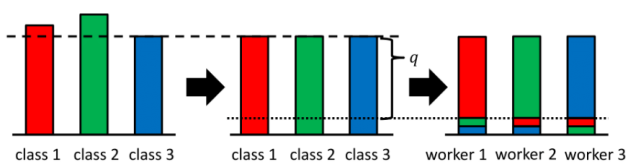
Figure 1: An illustraion of our local datasets generation process.

Models. We conducted our experiments using an one-hidden layer fully connected neural network with $100$ hidden units and softplus activation. For loss function, we used the standard cross-entropy loss. We initialized parameters by uniformly sampling the parameters from $[-\sqrt{6/(n_{\mathrm{in}}+n_{\mathrm{out}})},\sqrt{6/(n_{\mathrm{in}}+n_{\mathrm{out}})}]$ (Glorot & Bengio, 2010), where $n_{\mathrm{in}}$ and $n_{\mathrm{out}}$ are the number of units in the input and output layers respectively. Furthermore, we add $L_{2}$-regularizer to the empirical risk with fixed regularization parameter $5\times 10^{-3}$.

Implemented Algorithms. We implemented minibatch SGD, Local SGD, SARAH, SCAFFOLD and our BVR-L-SGD. For each local computation budget $\mathcal{B}\in\{256,512,1024\}$, we set $K=\mathcal{B}/16$ and $b=16$ for local methods (Local SGD, SCAFFOLD and BVR-L-SGD), and $b=\mathcal{B}$ for non-local ones (minibatch SGD and SARAH). Note that each algorithm requires the same order of stochastic gradient computations per communication. For each algorithm, we tuned learning rate $\eta$ from $\{0.005,0.01,0.05,0.1,0.5,1.0\}$. The details of the tuning procedure are found in the supplementary material (Section D).

Evaluation. We compared the implemented algorithms using four criteria of train loss; train accuracy; test loss and test accuracy against (i) heterogeneity $q$; (ii) local computation budgets $\mathcal{B}$ and (iii) the number of communication rounds. The total number of communication rounds was fixed to $3,000$ for each algorithm. We independently repeated the experiments $5$ times and report the mean and standard deviation of the above criteria. Due to the space limitation, we will only report train loss and test accuracy in the main paper. The full results are found in the supplementary material (Section D).

Results 1: Effect of the heterogeneity. Here, we investigate the effect of the heterogeneity on the convergence speed of the algorithms. To clarify the pure effect of the heterogeneity, we fixed the local computation budget $\mathcal{B}$ to $1,024$, which was the largest one in our experiments. Figure 2 shows the comparison of the best-achieved train loss and test accuracy in $3,000$ communication rounds against heterogeneity parameter $q$. From this, we can see that the convergence speed of the local methods deteriorated as heterogeneity parameter $q$ increased. Particularly, the degree of the performance degradation of L-SGD and SCAFFOLD was serious. In contrast, this phenomenon was not observed for non-local methods, because the convergence rates of non-local methods do not depend on heterogeneity $\zeta$ as in Table 1. Importantly, even for the largest $q$, BVR-L-SGD significantly outperformed the other methods.

2

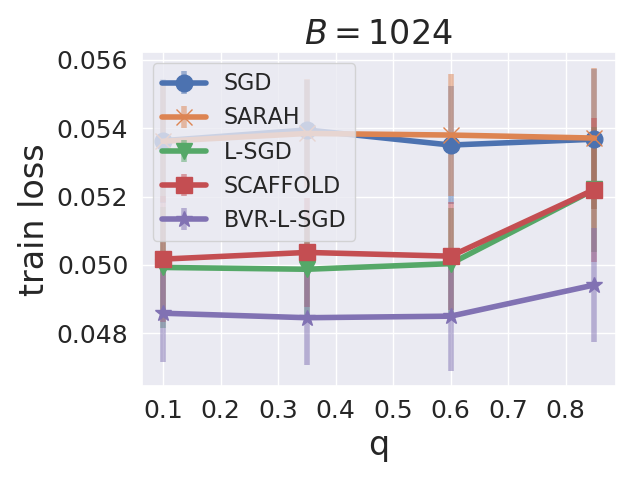
(a) Best Train Loss

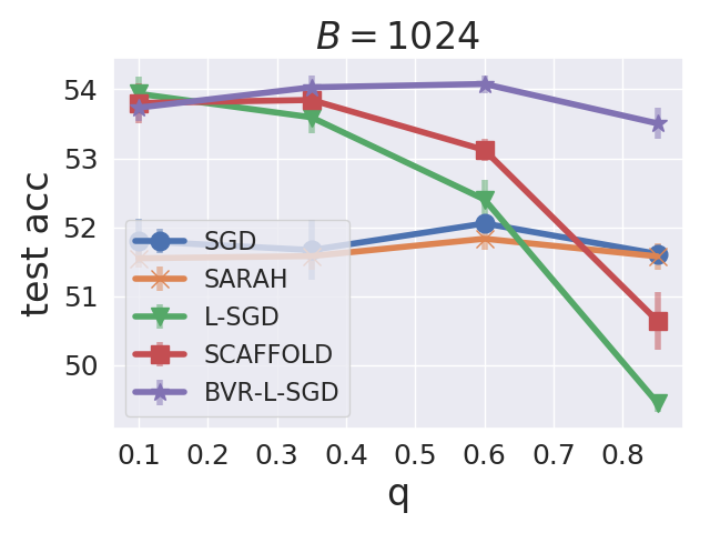
(b) Best Test Accuracy

Figure 2: Comparison of the best train loss and test accuracy against heterogeneity parameter $q$.

Results 2: Effect of the local computation budget size. Now, we examine the effect of the size of the local computation budget $\mathcal{B}$ to the convergence speed. For this purpose, we fixed heterogeneity parameter $q$ to the smallest one. Figure 3 shows the comparison of the best-achieved train loss and test accuracy against local computation budget $\mathcal{B}$. We can see that the local methods improved their performances as local computation budget $\mathcal{B}$ increased, but non-local methods did not. This is because local methods can potentially achieve a smaller communication complexity than $1/\varepsilon$ by increasing $\mathcal{B}$ for small $\zeta$, but non-local methods can not break the barrier of $1/\varepsilon$ for any $\mathcal{B}$ as in Table 1.

2

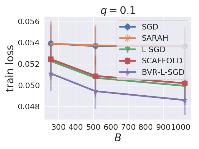
(a) Best Train Loss

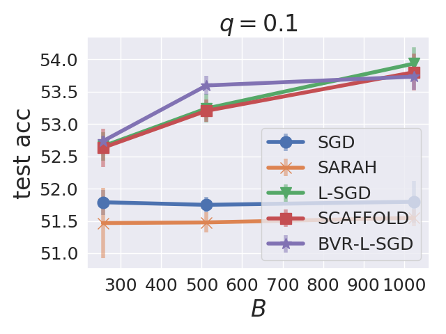
(b) Best Test Accuracy

Figure 3: Comparison of the best train loss and test accuracy against local computation budget $\mathcal{B}$.

Results 3: Effect of the number of communication rounds. Finally, to see the trends of train loss and test accuracy during optimization, we give the comparison of the train loss and test accuracy against the number of communication rounds (Figure 4). For the space limitation, we only report the case $\mathcal{B}=1,024$. From these results, it can be seen that our proposed BVR-L-SGD consistently outperformed the other methods from beginning to end.

2 2 2 2

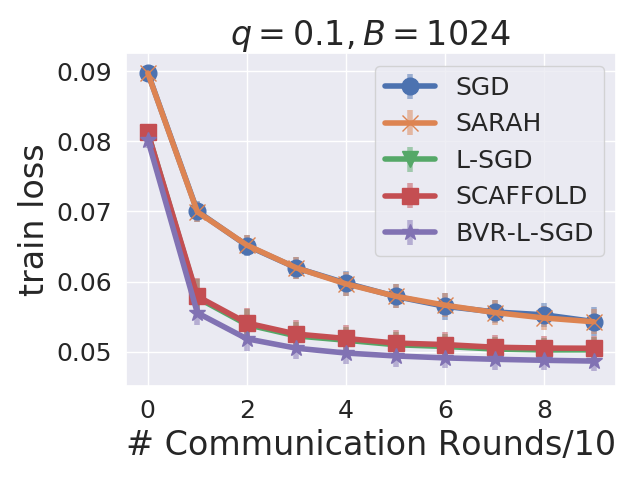
(a) Train Loss

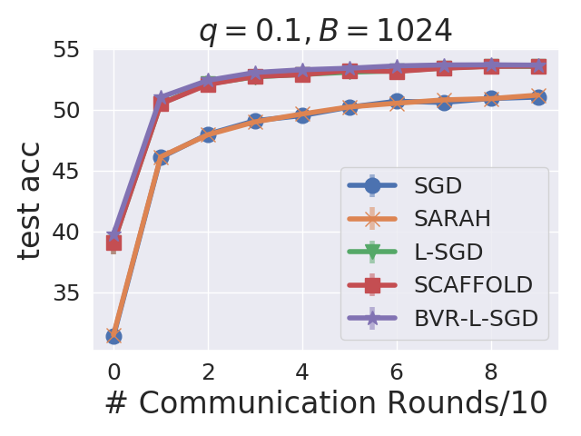
(b) Test Accuracy

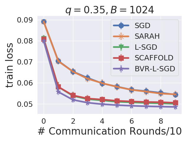
(c) Train Loss

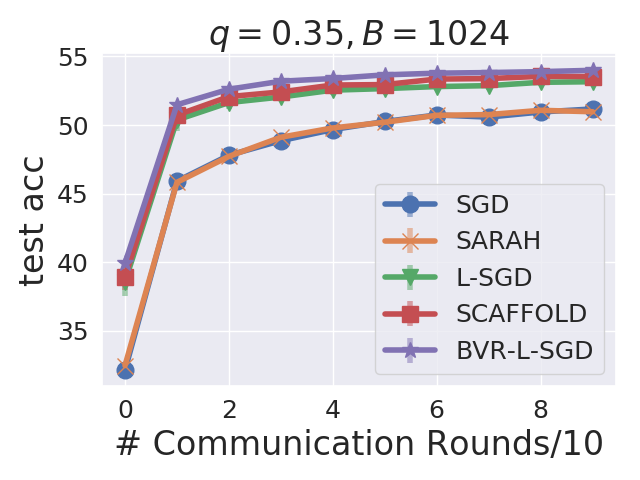
(d) Test Accuracy

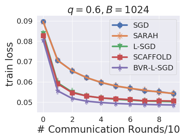
(e) Train Loss

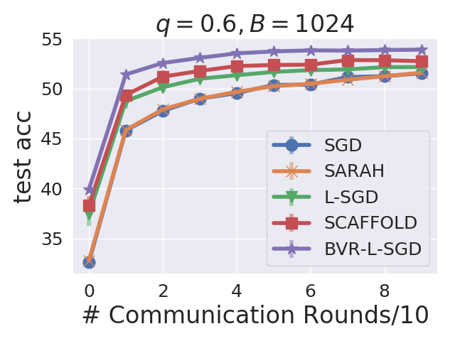
(f) Test Accuracy

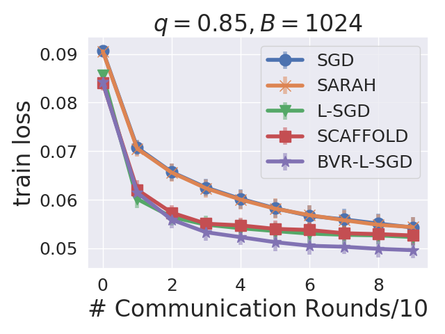
(g) Train Loss

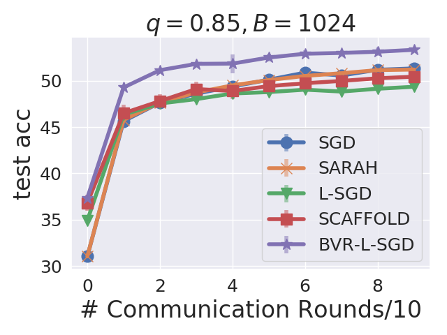
(h) Test Accuracy

Figure 4: Comparison of the train loss and test accuracy against the number of communication rounds.

In summary, for small heterogeneity, local methods significantly surpassed non-local methods. For relatively large heterogeneity, the performances of the existing local methods were seriously degraded. In contrast, the degree of deterioration of BVR-L-SGD was small and BVR-L-SGD consistently out-performed both the existing non-local and local methods. These observations strongly verify the theoretical findings and showed the empirical superiority of our method.

6 Conclusion and Future Work

In this paper, we studied our proposed BVR-L-SGD for nonconvex distributed learning, which is based on the bias-variance reduced gradient estimator to fully utilize the small second-order heterogeneity of local objectives and suggests randomly picking up one of the local models instead of taking the average of them when workers are synchronized. Our theory implies the superiority of BVR-L-SGD to previous non-local and local methods in terms of communication complexity. The numerical results strongly encouraged our theoretical results and suggested the empirical superiority of the proposed method.

One promising and challenging future work is to extend our algorithm and theory to the problem of finding second-order stationary points. Although there are many papers for finding second-order stationary points for general nonconvex problems (Ge et al., 2015; Allen-Zhu, 2017; Jin et al., 2017; Li, 2019), it might be inherently difficult for local algorithms to efficiently find a local minima due to the nature of local updates. An open question is that: can we construct a local algorithm that guarantees to find second-order stationary points and is more communication efficient than non-local methods for local objectives with small heterogeneity?

Appendix A Analysis of Local-Routine (Algorithm 3)

In this section, we give the analysis of Local-Routine.

Proof of Lemma 4.1

Let $\eta_{1}=1/(4L)$. From $L$-smoothness of $f$, we have

$$f(x_{k}^{(p)})\leq \ f(x_{k-1}^{(p)})+\langle\nabla f(x_{k-1}^{(p)}),x_{k}^{(p)}-x_{k-1}^{(p)}\rangle+\frac{L}{2}\|x_{k}^{(p)}-x_{k-1}^{(p)}\|^{2}$$

$$= \ f(x_{k-1}^{(p)})-\eta\langle\nabla f(x_{k-1}^{(p)}),v_{k}^{(p)}\rangle+\frac{\eta^{2}L}{2}\|v_{k}^{(p)}\|^{2}$$

$$\leq \ f(x_{k-1}^{(p)})-\eta\|\nabla f(x_{k-1}^{(p)})\|^{2}-\eta\langle\nabla f(x_{k-1}^{(p)}),v_{k}^{(p)}-\nabla f(x_{k-1}^{(p)})\rangle+\eta^{2}L\|v_{k}^{(p)}-\nabla f(x_{k-1}^{(p)})\|^{2}$$

$$+\eta^{2}L\|\nabla f(x_{k-1}^{(p)})\|^{2}$$

$$\leq \ f(x_{k-1}^{(p)})-\eta\left(\frac{3}{4}-\frac{\eta}{L}\right)\|\nabla f(x_{k-1}^{(p)})\|^{2}+\eta\left(1+\eta L\right)\|v_{k}^{(p)}-\nabla f(x_{k-1}^{(p)})\|^{2}$$

$$\leq \ f(x_{k-1}^{(p)})-\frac{\eta}{2}\|\nabla f(x_{k-1}^{(p)})\|^{2}+\eta\left(1+\eta L\right)\|v_{k}^{(p)}-\nabla f(x_{k-1}^{(p)})\|^{2}.$$

Here, in the second and third inequalities we used Cauchy Schwarz inequality and Arithmetic Mean-Geometric Mean inequality. The last inequality holds because $\eta\leq 1/(4L)$. Hence, we get

$$\|\nabla f(x_{k-1}^{(p)})\|^{2}\leq \ \frac{2}{\eta}(f(x_{k-1}^{(p)})-f(x_{k}^{(p)}))+2(1+\eta L)\|v_{k}^{(p)}-\nabla f(x_{k-1}^{(p)})\|^{2}$$

$$\leq \ \frac{2}{\eta}(f(x_{k-1}^{(p)})-f(x_{k}^{(p)}))+\frac{5}{2}\|v_{k}^{(p)}-\nabla f(x_{k-1}^{(p)})\|^{2}.$$

Finally, taking expectation on both sides yields the desired result. ∎

Lemma A.1.

Local-Routine($p$, $x_{0}$, $\eta$, $v_{0}$, $b$, $K$) satisfies for $k\in[K]$,

$$\mathbb{E}\|x_{k}^{(p)}-x_{0}\|^{2}\leq\Theta(\eta^{2}K^{2})\frac{1}{K}\sum_{k^{\prime}=1}^{K}\mathbb{E}\|v_{k^{\prime}}^{(p)}-\nabla f(x_{k^{\prime}-1}^{(p)})\|^{2}+\Theta(\eta^{2}K^{2})\frac{1}{K}\sum_{k^{\prime}=1}^{K}\mathbb{E}\|\nabla f(x_{k^{\prime}-1}^{(p)})\|^{2}.$$

for $p\in[P]$ and $k\in[K]$.

Proof.

$$\|x_{k}^{(p)}-x_{0}\|^{2}$$

$$= \ \|x_{k-1}^{(p)}-x_{0}+\eta v_{k}^{(p)}\|^{2}$$

$$\leq \ \left(1+\frac{1}{K}\right)\|x_{k-1}^{(p)}-x_{0}\|^{2}+\eta^{2}(1+K)\|v_{k}^{(p)}\|^{2}$$

$$\leq \ \left(1+\frac{1}{K}\right)\|x_{k-1}^{(p)}-x_{0}\|^{2}+2\eta^{2}(1+K)\|v_{k}^{(p)}-\nabla f(x_{k-1}^{(p)})\|^{2}+2\eta^{2}K\|\nabla f(x_{k-1}^{(p)})\|^{2}.$$

Here, the inequality follows from Cauchy Schwarz inequality and Arithmetic Mean-Geometric Mean inequality. Recursively using this inequality, we obtain

$$\|x_{k}^{(p)}-x_{0}\|^{2}$$

$$\leq \ 2\eta^{2}(1+K)\sum_{k^{\prime}=1}^{k}\left(1+\frac{1}{K}\right)^{k-k^{\prime}}\|v_{k^{\prime}}^{(p)}-\nabla f(x_{k^{\prime}-1}^{(p)})\|^{2}+2\eta^{2}(1+K)\sum_{k^{\prime}=1}^{k}\left(1+\frac{1}{K}\right)^{k-k^{\prime}}\|\nabla f(x_{k^{\prime}-1}^{(p)})\|^{2}$$

$$\leq \ 2e\eta^{2}(1+K)\sum_{k^{\prime}=1}^{K}\|v_{k^{\prime}}^{(p)}-\nabla f(x_{k^{\prime}-1}^{(p)})\|^{2}+2e\eta^{2}(1+K)\sum_{k^{\prime}=1}^{K}\|\nabla f(x_{k^{\prime}-1}^{(p)})\|^{2}.$$

Here, we used the fact that $(1+1/K)^{k-k^{\prime}}\leq(1+1/K)^{K}\leq e$ and the definition $x_{0}^{(p)}=x_{0}$. ∎

Lemma A.2.

Suppose that Assumptions and 1 hold. Then, for any $x,y\in\mathbb{R}^{d}$,

$$\|\nabla f_{p}(x)-\nabla f_{p}(y)+\nabla f(y)-\nabla f(x)\|^{2}\leq\zeta^{2}\|x-y\|^{2}$$

for $p\in[P]$.

Proof.

From the convexity of $\|\cdot\|^{2}$, we have

$$\|\nabla f_{p}(x)-\nabla f_{p}(y)+\nabla f(y)-\nabla f(x)\|^{2}$$

$$\leq \ \frac{1}{P}\sum_{p^{\prime}\neq p}\|\nabla f_{p}(x)-\nabla f_{p}(y)+\nabla f_{p^{\prime}}(y)-\nabla f_{p^{\prime}}(x)\|^{2}.$$

Since $f_{p}-f_{p^{\prime}}$ is $C^{2}$- function, $\nabla f_{p}(x)-\nabla f_{p^{\prime}}(x)-\nabla f_{p}(y)+\nabla f_{p^{\prime}}(y)=\nabla(f_{p}-f_{p^{\prime}})(x)-\nabla(f_{p}-f_{p^{\prime}})(y)=(\nabla^{2}(f_{p}-f_{p^{\prime}})(\xi))(x-y)$ for some $\xi\in\mathbb{R}^{d}$ by Mean value theorem. Hence, we have

$$\|\nabla f_{p}(x)-\nabla f_{p}(y)+\nabla f_{p^{\prime}}(y)-\nabla f_{p^{\prime}}(x)\|^{2}$$

$$\leq \ \frac{1}{P}\sum_{p^{\prime}\neq p}\|\nabla^{2}f_{p}(\xi)-\nabla^{2}f_{p^{\prime}}(\xi)\|_{2}^{2}\|x-y\|^{2}$$

$$\leq \ \zeta^{2}\|x-y\|^{2}.$$

Here the last inequality holds thanks to Assumption 1. ∎

Proof of Lemma 4.2

Observe that

$$\mathbb{E}\|v_{k}^{(p)}-\nabla f(x_{k-1}^{(p)})\|^{2}$$

$$= \ \mathbb{E}\|g_{k}^{(p)}(x_{k-1}^{(p)})-g_{k}^{(p)}(x_{k-2}^{(p)})+v_{k-1}^{(p)}-\nabla f(x_{k-1}^{(p)})\|^{2}$$

$$= \ \mathbb{E}\|g_{k}^{(p)}(x_{k-1}^{(p)})-g_{k}^{(p)}(x_{k-2}^{(p)})-\nabla f_{p}(x_{k-1}^{(p)})+\nabla f_{p}(x_{k-2}^{(p)})\|^{2}$$

$$+\mathbb{E}\|\nabla f_{p}(x_{k-1}^{(p)})-\nabla f_{p}(x_{k-1}^{(p)})+v_{k-1}^{(p)}-\nabla f(x_{k-1}^{(p)})\|^{2}$$

$$\leq \ \mathbb{E}\|g_{k}^{(p)}(x_{k-1}^{(p)})-g_{k}^{(p)}(x_{k-2}^{(p)})-\nabla f_{p}(x_{k-1})+\nabla f_{p}(x_{k-2}^{(p)})\|^{2}$$

$$+(1+K)\mathbb{E}\|\nabla f_{p}(x_{k-1})-\nabla f_{p}(x_{k-2}^{(p)})+\nabla f(x_{k-2}^{(p)})-\nabla f(x_{k-1}^{(p)})\|^{2}$$

$$+\left(1+\frac{1}{K}\right)\mathbb{E}\|v_{k-1}^{(p)}-\nabla f(x_{k-2}^{(p)})\|^{2}$$

$$\leq \ \frac{1}{b}\mathbb{E}\left[\mathbb{E}_{z\sim\mathcal{D}_{p}}\|\nabla\ell(x_{k-1}^{(p)},z)-\nabla\ell(x_{k-2}^{(p)},z)\|^{2}\right]$$

$$+(1+K)\mathbb{E}\|\nabla f_{p}(x_{k-1}^{(p)})-\nabla f_{p}(x_{k-2}^{(p)})+\nabla f(x_{k-2}^{(p)})-\nabla f(x_{k-1}^{(p)})\|^{2}$$

$$+\left(1+\frac{1}{K}\right)\mathbb{E}\|v_{k-1}^{(p)}-\nabla f(x_{k-2}^{(p)})\|^{2}.$$

Here, the second equality holds because $\mathbb{E}[g_{k}^{(p)}(x_{k-1}^{(p)})]=\nabla f_{p}(x_{k-1}^{(p)})$ and $\mathbb{E}[g_{k}^{(p)}(x_{k-2}^{(p)})]=\nabla f_{p}(x_{k-2}^{(p)})$. The fist inequality is from Cauchy-Schwarz inequlality and Arithmetic Mean-Geometric Mean inequality. The last inequality follows from the fact that $g_{k}^{(p)}$ constituted by $b$ IID stochastic gradients. Recursively using this inequality, we have

$$\mathbb{E}\|v_{k}^{(p)}-\nabla f(x_{k-1}^{(p)})\|^{2}$$

$$\leq \ \frac{eK}{b}\frac{1}{K}\sum_{k^{\prime}=1}^{K}\mathbb{E}\left[\mathbb{E}_{z\sim\mathcal{D}_{p}}\|\nabla\ell(x_{k^{\prime}-1}^{(p)},z)-\nabla\ell(x_{k^{\prime}-2}^{(p)},z)\|^{2}\right]$$

$$+e(1+K)K\frac{1}{K}\sum_{k^{\prime}=1}^{K}\mathbb{E}\|\nabla f_{p}(x_{k^{\prime}-1}^{(p)})-\nabla f_{p}(x_{k^{\prime}-2}^{(p)})+\nabla f(x_{k^{\prime}-2}^{(p)})-\nabla f(x_{k^{\prime}-1}^{(p)})\|^{2}$$

$$+e\|v_{0}-\nabla f(x_{0})\|^{2}.$$

Note that $x_{0}^{(p)}=x_{0}$ and $v_{0}^{(p)}=v_{0}$. Then applying Lemma A.2, we get

$$\mathbb{E}\|v_{k}^{(p)}-\nabla f(x_{k-1}^{(p)})\|^{2}\leq \ \Theta\left(\frac{K}{b}\right)\frac{1}{K}\sum_{k^{\prime}=1}^{K}\mathbb{E}[\mathbb{E}_{z\sim\mathcal{D}_{p}}\|\nabla\ell(x_{k^{\prime}-1}^{(p)},z)-\nabla\ell(x_{k^{\prime}-2}^{(p)},z)\|^{2}]$$

$$+\Theta(\zeta^{2}K^{2})\frac{1}{K}\sum_{k^{\prime}=1}^{K}\mathbb{E}\|x_{k^{\prime}-1}^{(p)}-x_{k^{\prime}-2}^{(p)}\|^{2}$$

$$+\Theta(1)\|v_{0}-\nabla f(x_{0})\|^{2}$$

$$\leq \ \Theta\left(\frac{L^{2}K}{b}+\zeta^{2}K^{2}\right)\frac{1}{K}\sum_{k^{\prime}=1}^{K}\mathbb{E}\|x_{k^{\prime}-1}^{(p)}-x_{k^{\prime}-2}^{(p)}\|^{2}$$

$$+\Theta(1)\|v_{0}-\nabla f(x_{0})\|^{2}$$

$$\leq \ \Theta\left(\frac{\eta^{2}L^{2}K}{b}+\eta^{2}\zeta^{2}K^{2}\right)\frac{1}{K}\sum_{k^{\prime}=1}^{K}\mathbb{E}\|v_{k^{\prime}-1}^{(p)}-\nabla f(x_{k^{\prime}-1}^{(p)})\|^{2}$$

$$+\Theta\left(\frac{\eta^{2}L^{2}K}{b}+\eta^{2}\zeta^{2}K^{2}\right)\frac{1}{K}\sum_{k^{\prime}=1}^{K}\mathbb{E}\|\nabla f(x_{k^{\prime}-1}^{(p)})\|^{2}$$

$$+\Theta(1)\|v_{0}-\nabla f(x_{0})\|^{2}.$$

Here, The second inequality holds by Assumption 2. Averaging this inequality from $k=1$ to $K$ and choosing sufficiently small $\eta_{2}$ such that $\eta_{2}=\Theta(1/(K\zeta)\wedge\sqrt{b}/(\sqrt{K}L))$, for any $\eta\leq\eta_{2}^{\prime}$, the factor $\Theta(\eta^{2}L^{2}K/b+\eta^{2}\zeta^{2}K^{2})$ becomes smaller than $1/2$. This gives the desired result. ∎

Proof of Proposition 4.3

From Lemma 4.1, we have

$$\frac{1}{K}\sum_{k=1}^{K}\mathbb{E}\|\nabla f(x_{k-1}^{(p)})\|^{2}\leq\Theta\left(\frac{1}{\eta K}\right)(\mathbb{E}f(x_{0})-\mathbb{E}f(x_{K}^{(p)}))+\Theta(1)\frac{1}{K}\sum_{k=1}^{K}\mathbb{E}\|v_{k}^{(p)}-\nabla f(x_{k-1}^{(p)})\|^{2}.$$

Applying Lemma 4.2 to this inequality, there exists $\eta_{3}=\Theta((1/L)\wedge\eta_{2})$, where $\eta_{2}$ is defined in Lemma 4.2, such that for every $\eta\leq\eta_{3}$, we get

$$\frac{1}{K}\sum_{k=1}^{K}\mathbb{E}\|\nabla f(x_{k-1}^{(p)})\|^{2}\leq\Theta\left(\frac{1}{\eta K}\right)(\mathbb{E}f(x_{0})-\mathbb{E}f(x_{K}^{(p)}))+\Theta(1)\|v_{0}-\nabla f(x_{0})\|^{2}.$$

Finally, since $\hat{k}\sim\mathrm{Unif}[K]$, taking expectation with respect to $\hat{k}$ gives the desired result. ∎

Appendix B Analysis of BVR-L-SGD (Algorithm 2)

In this section, we provide the analysis of BVR-L-SGD.

Proof of Lemma 4.4

We define $V_{t}^{(p)}$ as $\frac{1}{K}\sum_{k=1}^{K}\mathbb{E}\|v_{k}^{(p)}-\nabla f(x_{k-1}^{(p)})\|^{2}$ in Local-Routine at iteration $t$. Then, we can rewrite the statement in Lemma 4.2 as

$$V_{t}^{(p)}\leq\Theta\left(\frac{\eta^{2}L^{2}K}{b}+\eta^{2}\zeta^{2}K^{2}\right)\mathbb{E}\left\|\nabla f(x_{t}^{(p),\mathrm{out}})\right\|^{2}+\Theta(1)\|\widetilde{v}_{t}-\nabla f(x_{t-1})\|^{2}.$$

Averaging this inequality from $p=1$ to $P$, we have

$$\frac{1}{P}\sum_{p=1}^{P}V_{t}^{(p)}\leq\Theta\left(\frac{\eta^{2}L^{2}K}{b}+\eta^{2}\zeta^{2}K^{2}\right)\frac{1}{P}\sum_{p=1}^{P}\mathbb{E}\left\|\nabla f(x_{t}^{(p),\mathrm{out}})\right\|^{2}+\Theta(1)\|\widetilde{v}_{t}-\nabla f(x_{t-1})\|^{2}.$$ (1)

Observe that

$$\mathbb{E}\|\widetilde{v}_{t}-\nabla f(x_{t-1})\|^{2}$$

$$= \ \mathbb{E}\left\|\frac{1}{P}\sum_{p=1}^{P}\left(g_{t}^{(p)}(x_{t-1})-g_{t}^{(p)}(x_{t-2})+\widetilde{v}_{t-1}^{(p)}\right)-\nabla f(x_{t-1})\right\|^{2}$$

$$= \ \mathbb{E}\left\|\frac{1}{P}\sum_{p=1}^{P}\left(g_{t}^{(p)}(x_{t-1})-g_{t}^{(p)}(x_{t-2})\right)-\nabla f(x_{t-1})+\nabla f(x_{t-2})\right\|^{2}+\mathbb{E}\|\widetilde{v}_{t-1}-\nabla f(x_{t-2})\|^{2}$$

$$= \ \frac{1}{P^{2}}\sum_{p=1}^{P}\mathbb{E}\left\|g_{t}^{(p)}(x_{t-1})-g_{t}^{(p)}(x_{t-2})-\nabla f_{p}(x_{t-1})+\nabla f_{p}(x_{t-2})\right\|^{2}+\mathbb{E}\|\widetilde{v}_{t-1}-\nabla f(x_{t-2})\|^{2}$$

$$\leq \ \frac{1}{PKb}\frac{1}{P}\sum_{p=1}^{P}\mathbb{E}\left[\mathbb{E}_{z\sim D_{p}}\left\|\nabla\ell(x_{t-1},z)-\nabla\ell(x_{t-2},z)\right\|^{2}\right]+\mathbb{E}\|\widetilde{v}_{t-1}-\nabla f(x_{t-2})\|^{2}.$$

Here, the second inequality holds from $\mathbb{E}[g_{t}^{(p)}(x_{t-1})|t-1]=\nabla f_{p}(x_{t-1})$ and $\mathbb{E}[g_{t}^{(p)}(x_{t-2})|t-1]=\nabla f_{p}(x_{t-2})$. The last equality is from the independency of $g_{t}^{(p)}(x_{t-1})-g_{t}^{(p)}(x_{t-2})$ given the history of the iterations $1,\ldots,t-1$. The last inequality holds because the $Kb$ samples used for $g_{t}^{(p)}(x_{t-1})$ and $g_{t}^{(p)}(x_{t-2})$ are IID. Recursively using this inequality, we have

$$\mathbb{E}\|\widetilde{v}_{t}-\nabla f(x_{t-1})\|^{2}$$

$$\leq \ \frac{T}{PKb}\frac{1}{T}\sum_{t^{\prime}=1}^{T}\frac{1}{P}\sum_{p=1}^{P}\mathbb{E}\left[\mathbb{E}_{z\sim D_{p}}\left\|\nabla\ell(x_{t^{\prime}-1},z)-\nabla\ell(x_{t^{\prime}-2},z)\right\|^{2}\right]+\mathbb{E}\|\widetilde{v}_{0}-\nabla f(x_{0})\|^{2}$$

$$\leq \ \frac{L^{2}T}{PKb}\frac{1}{T}\sum_{t^{\prime}=1}^{T}\mathbb{E}\left\|x_{t^{\prime}-1}-x_{t^{\prime}-2}\right\|^{2}+\mathds{1}_{\widetilde{b}<\frac{1}{P}\sum_{p=1}^{P}\#\mathrm{supp}(D_{p})}\frac{\sigma^{2}}{P\widetilde{b}}.$$

The last inequality follows from Assumptions 2 and 4 with the definition of $\widetilde{v}_{0}$. From Lemma A.1, we have

$$\mathbb{E}\|x_{t^{\prime}}-x_{t^{\prime}-1}\|^{2}\leq\Theta(\eta^{2}K^{2})\frac{1}{P}\sum_{p=1}^{P}(V_{t^{\prime}}^{(p)}+\mathbb{E}\|\nabla f(x_{t^{\prime}}^{(p),\mathrm{out}})\|^{2}).$$

Hence, we get

$$\frac{1}{T}\sum_{t=1}^{T}\mathbb{E}\|\widetilde{v}_{t}-\nabla f(x_{t-1})\|^{2}$$

$$\leq \ \frac{L^{2}T}{PKb}\frac{1}{T}\sum_{t^{\prime}=1}^{T}\mathbb{E}\left\|x_{t^{\prime}-1}-x_{t^{\prime}-2}\right\|^{2}+\mathds{1}_{\widetilde{b}<\frac{1}{P}\sum_{p=1}^{P}\#\mathrm{supp}(D_{p})}\frac{\sigma^{2}}{P\widetilde{b}}$$

$$\leq \ \frac{\eta^{2}L^{2}KT}{Pb}\frac{1}{T}\sum_{t^{\prime}=1}^{T}\frac{1}{P}\sum_{p=1}^{P}V_{t^{\prime}}^{(p)}+\frac{\eta^{2}L^{2}KT}{Pb}\frac{1}{T}\sum_{t^{\prime}=1}^{T}\frac{1}{P}\sum_{p=1}^{P}\mathbb{E}\|\nabla f(x_{t^{\prime}-1}^{(p),\mathrm{out}})\|^{2}+\mathds{1}_{\widetilde{b}<\frac{1}{P}\sum_{p=1}^{P}\#\mathrm{supp}(D_{p})}\frac{\sigma^{2}}{P\widetilde{b}}.$$

Choosing $\eta_{4}\leq\eta_{3}$ such that $\Theta(\eta_{4}^{2}L^{2}KT/Pb)<1/2$, for every $\eta\leq\eta_{4}$, combining (1) yields

$$\frac{1}{T}\sum_{t=1}^{T}\mathbb{E}\|\widetilde{v}_{t}-\nabla f(x_{t-1})\|^{2}$$

$$\leq \ \Theta\left(\frac{\eta^{2}L^{2}K}{b}+\eta^{2}\zeta^{2}K^{2}+\frac{\eta^{2}L^{2}KT}{Pb}\right)\frac{1}{T}\sum_{t^{\prime}=1}^{T}\frac{1}{P}\sum_{p=1}^{P}\mathbb{E}\|\nabla f(x_{t^{\prime}-1}^{(p),\mathrm{out}})\|^{2}+\mathds{1}_{\widetilde{b}<\frac{1}{P}\sum_{p=1}^{P}\#\mathrm{supp}(D_{p})}\frac{\sigma^{2}}{P\widetilde{b}}.$$

This is the desired result. ∎

Proof of Theorem 4.5

The statement of Proposition 4.3 at iteration $t$ implies

$$\frac{1}{P}\sum_{p=1}^{P}\mathbb{E}\|\nabla f(x_{t}^{(p),\mathrm{out}})\|^{2}\leq\Theta\left(\frac{1}{\eta K}\right)(\mathbb{E}f(x_{t-1})-\mathbb{E}f(x_{t}))+\Theta(1)\mathbb{E}\|\widetilde{v}_{t}-\nabla f(x_{t-1})\|^{2}.$$

Averaging this inequality from $t=1$ to $T$ results in

$$\frac{1}{T}\sum_{t=1}^{T}\frac{1}{P}\sum_{p=1}^{P}\mathbb{E}\|\nabla f(x_{t}^{(p),\mathrm{out}})\|^{2}\leq\Theta\left(\frac{1}{\eta TK}\right)(\mathbb{E}f(x_{0})-\mathbb{E}f(x_{T}))+\Theta(1)\frac{1}{T}\sum_{t=1}^{T}\mathbb{E}\|\widetilde{v}_{t}-\nabla f(x_{t-1})\|^{2}.$$

Then, applying Lemma 4.4 to this inequality, there exists $\eta=\Theta(1/L\wedge 1/(K\zeta)\wedge\sqrt{b}/(\sqrt{K}L)\wedge\sqrt{Pb}/(\sqrt{KT}L)$ such that

$$\frac{1}{T}\sum_{t=1}^{T}\frac{1}{P}\sum_{p=1}^{P}\mathbb{E}\|\nabla f(x_{t}^{(p),\mathrm{out}})\|^{2}\leq\Theta\left(\frac{1}{\eta KT}\right)(\mathbb{E}f(x_{0})-\mathbb{E}f(x_{T}))+\Theta(1)\mathds{1}_{\widetilde{b}<\frac{1}{P}\sum_{p=1}^{P}\#\mathrm{supp}(D_{p})}\frac{\sigma^{2}}{P\widetilde{b}}.$$

From the definitions of $\widetilde{x}_{s}$ and $\widetilde{x}_{s}^{\mathrm{out}}$, we obtain

$$\mathbb{E}\|\nabla f(\widetilde{x}_{s}^{\mathrm{out}})\|^{2}\leq\Theta\left(\frac{1}{\eta KT}\right)(\mathbb{E}f(\widetilde{x}_{s-1})-\mathbb{E}f(\widetilde{x}_{s}))+\Theta(1)\mathds{1}_{\widetilde{b}<\frac{1}{P}\sum_{p=1}^{P}\#\mathrm{supp}(D_{p})}\frac{\sigma^{2}}{P\widetilde{b}}.$$

Finally, averaging this inequality from $s=1$ to $S$ and using Assumption 3 yield the desired result. ∎

Corollary B.1.

Suppose that Assumptions 1, 2, 3 and 4 hold. We denote $n:=\sum_{p=1}^{P}\#\mathrm{supp}(D_{p})$. Let $\widetilde{b}=\Theta((n/P)\wedge(\sigma^{2}/(P\varepsilon)))$. Then, there exists $\eta=\Theta(1/L\wedge 1/(K\zeta)\wedge\sqrt{b}/(\sqrt{K}L)\wedge\sqrt{Pb}/(\sqrt{KT}L)))$ such that BVR-L-SGD($\widetilde{x}_{0}$, $\eta$, $b$, $\widetilde{b}$, $K$, $T$, $S$) with $S=\Theta(1+1/(\eta KT\varepsilon))$ satisfies

$$\mathbb{E}\|\nabla f(\widetilde{x}^{\mathrm{out}})\|^{2}\leq\Theta(\varepsilon).$$

Moreover, the total communication complexity $ST$ is

$$\Theta\left(\frac{L}{K\varepsilon}+\frac{\zeta}{\varepsilon}+\frac{L}{\sqrt{Kb}\varepsilon}+\sqrt{\frac{T}{KbP}}\frac{L}{\varepsilon}+T\right).$$

Remark (Communication efficiency).

Given local computation budget $\mathcal{B}$, we set $T=\Theta(1+\widetilde{b}/\mathcal{B})$ and $Kb=\Theta(\mathcal{B})$ with $b\leq\Theta(\sqrt{\mathcal{B}})$, where $\widetilde{b}$ was defined in Corollary B.1. Then, we have the averaged number of local computations per communication round $Kb+\widetilde{b}/T=\Theta(\mathcal{B})$ and the total communication complexity with budget $\mathcal{B}$ becomes $\Theta((L/(\sqrt{\mathcal{B}}\varepsilon)+\sqrt{n\wedge(\sigma^{2}/\varepsilon)}L/(\mathcal{B}P\varepsilon)+(n\wedge(\sigma^{2}/\varepsilon))/(\mathcal{B}P)+\zeta/\varepsilon)$.

Appendix C Practical Implementation of BVR-L-SGD

In this section, we give practical implementation details of BVR-L-SGD (Algorithm 4). The blue texts indicates the changes from the original algorithm (Algorithm 2) for more specific, and computational and communication efficient procedures.

In line 1, we set $T=\lceil 1+\widetilde{b}/(Kb)\rceil$, which has been theoretically determined. In line 16, we at first pick a worker $\hat{p}$ uniformly random and send aggregated variance reduced gradient $\widetilde{v}_{t}$ to it. Then, worker $\hat{p}$ runs Local-Routine using $\widetilde{v}_{t}$ (line 18). Central server receive its output and broadcast it to all the worker (line 19). Note that Algorithm 4 only requires single aggregation and single broadcast for each $t\in[T]$.

Algorithm 4 Practical Implementation of BVR-L-SGD($\widetilde{x}_{0}$, $\eta$, $b$, $\widetilde{b}$, $K$, $S$)

1:  Set $T=\lceil 1+\widetilde{b}/(Kb)\rceil$.

2:  for $s=1$ to $S$ do

3:     for $p=1$ to $P$ in parallel do

4:        if $\widetilde{b}\geq\frac{1}{P}\sum_{p=1}^{P}\#\mathrm{supp}(D_{p})$ then

5:           $\widetilde{\nabla}^{(p)}=\nabla f_{p}(\widetilde{x}_{s-1})$.

6:        else

7:           $\widetilde{\nabla}^{(p)}=\frac{1}{\widetilde{b}}\sum_{l=1}^{\widetilde{b}}\nabla\ell(\widetilde{x}_{s-1},z_{l})$ for $\widetilde{b}$ IID samples $z_{l}\sim D_{p}$.

8:        end if

9:     end for

10:     Central Server: aggregate $\{\widetilde{\nabla}^{(p)}\}_{p=1}^{P}$ and broadcast $\widetilde{v}_{0}=\frac{1}{P}\sum_{p=1}^{P}\widetilde{\nabla}^{(p)}$ to all the workers.

11:     Set $x_{0}=x_{-1}=\widetilde{x}_{s-1}$.

12:     for $t=1$ to $T$ do

13:        for $p=1$ to $P$ in parallel do

14:           $g_{t}^{(p)}(x_{t-1})=\frac{1}{Kb}\sum_{l=1}^{Kb}\ell(x_{t-1},z_{l})$ and $g_{t}^{(p)}(x_{t-2})=\frac{1}{Kb}\sum_{l=1}^{Kb}\ell(x_{t-2},z_{l})$ for $z_{l}\overset{i.i.d.}{\sim}D_{p}$.

15:           $\widetilde{v}_{t}^{(p)}=g_{t}^{(p)}(x_{t-1})-g_{t}^{(p)}(x_{t-2})+\widetilde{v}_{t-1}^{(p)}$.

16:        end for

17:        Pick $\hat{p}\sim[P]$ uniformly at random.

18:        Central Server: aggregate $\{\widetilde{v}_{t}^{(p)}\}_{p=1}^{P}$ and send $\widetilde{v}_{t}=\frac{1}{P}\sum_{p=1}^{P}\widetilde{v}_{t}^{(p)}$ to worker $\hat{p}$.

19:        $x_{t}^{(\hat{p})},\_=$ Local-Routine($\hat{p}$, $x_{t-1}$, $\eta$, $\widetilde{v}_{t}$, $b$, $K$)

20:        Central Server: receive $x_{t}^{(\hat{p})}$ and broadcast $x_{t}=x_{t}^{(\hat{p})}$ to all the workers.

21:     end for

22:     Set $\widetilde{x}_{s}=x_{T}$.

23:  end for

24:  Return: $\widetilde{x}^{\mathrm{out}}=\widetilde{x}_{S}$.

Appendix D Supplementary of Numerical Experiments

Parameter Tuning

For all the implemented algorithms, the only tuning parameter was learning rate $\eta$. We ran each algorithm with $\eta\in\{0.005,0.01,0.05,0.1,0.5,1.0\}$ and chose the one that maximized the minimum train accuracy at the last $100$ global iterates to take into account not only convergence speed but also stability of convergence.

Additional Numerical Results

Here, we provide the full results in our numerical experiments. Figures 5, 6 and 7 show the comparisons of train loss, train accuracy, test loss and test accuracy for various $q$ with fixed local computation budget $\mathcal{B}=256,512$ and $1,024$ respectively.

4 4 4 4

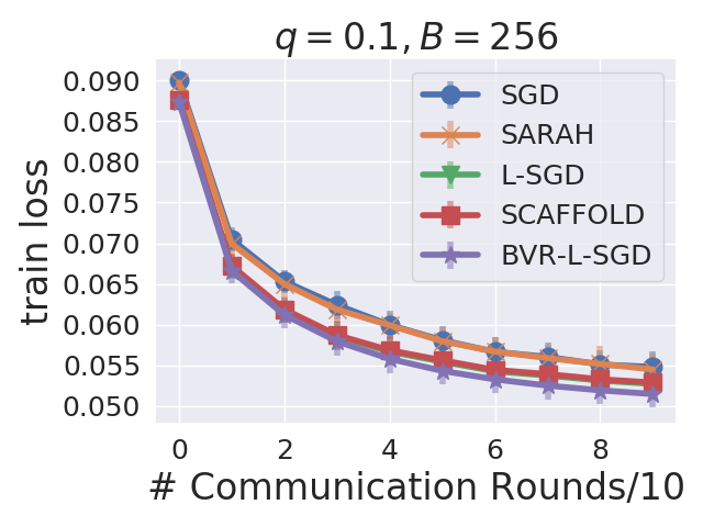
(a) Train Loss

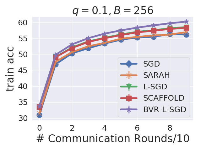
(b) Train Accuracy

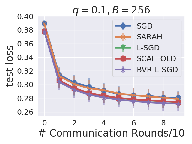
(c) Test Loss

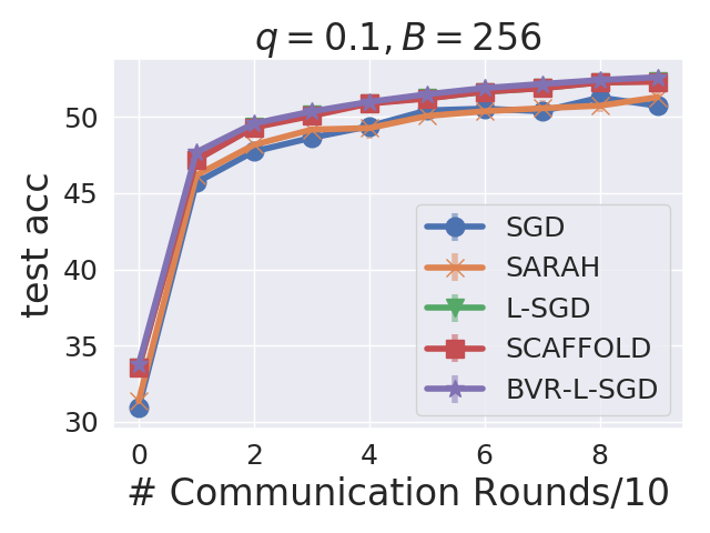
(d) Test Accuracy

(e) Train Loss

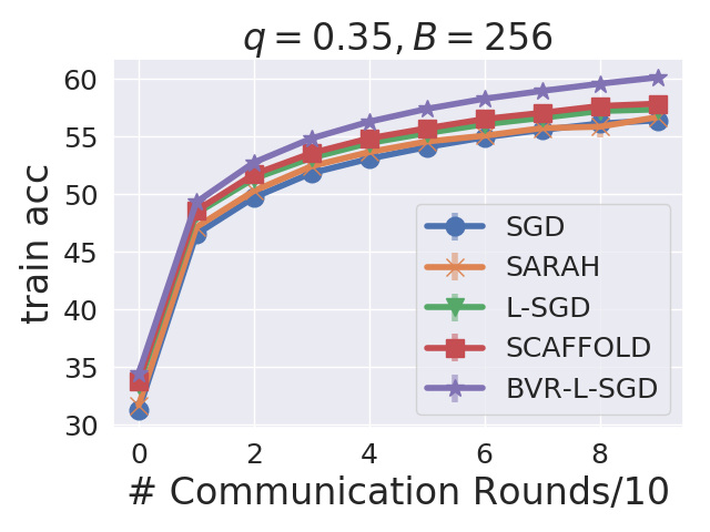
(f) Train Accuracy

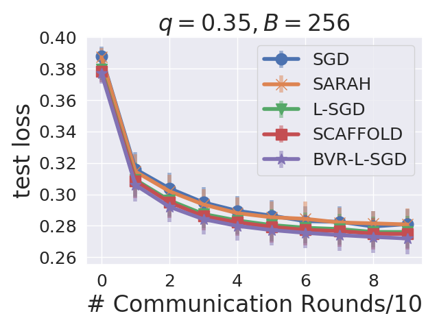
(g) Test Loss

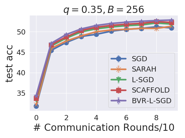
(h) Test Accuracy

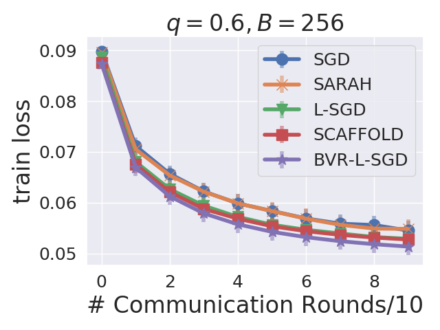
(i) Train Loss

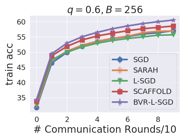
(j) Train Accuracy

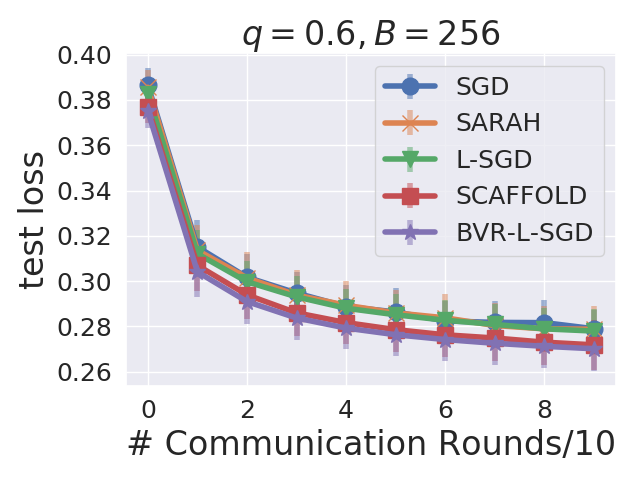
(k) Test Loss

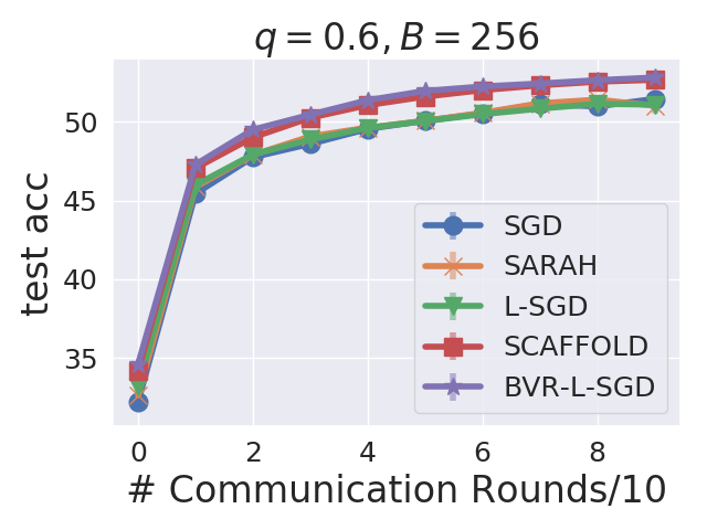
(l) Test Accuracy

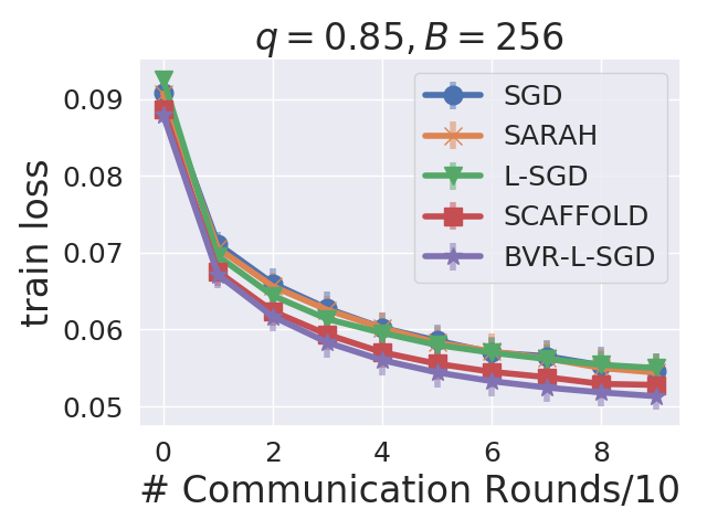
(m) Train Loss

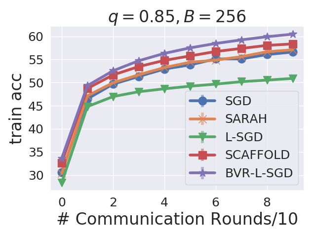
(n) Train Accuracy

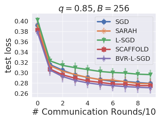
(o) Test Loss

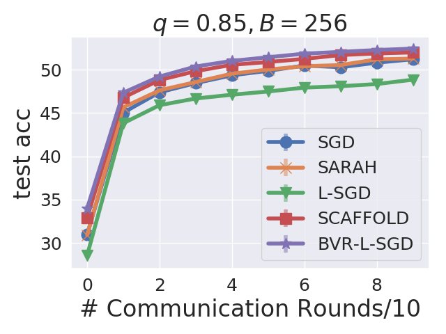
(p) Test Accuracy

Figure 5: Comparison of the train loss and test accuracy against the number of communication rounds for local computation budget $\mathcal{B}=256$.

4 4 4 4

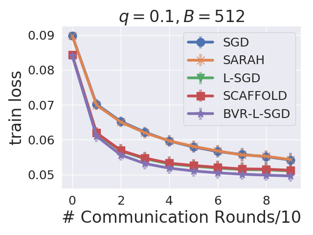
(a) Train Loss

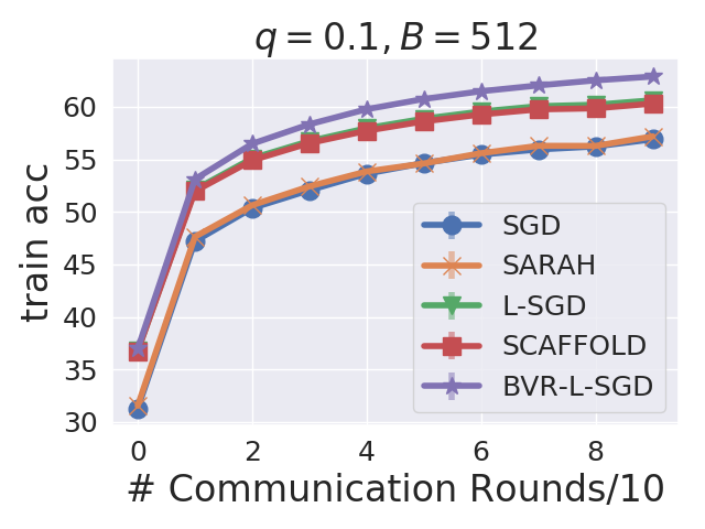
(b) Train Accuracy

(c) Test Loss

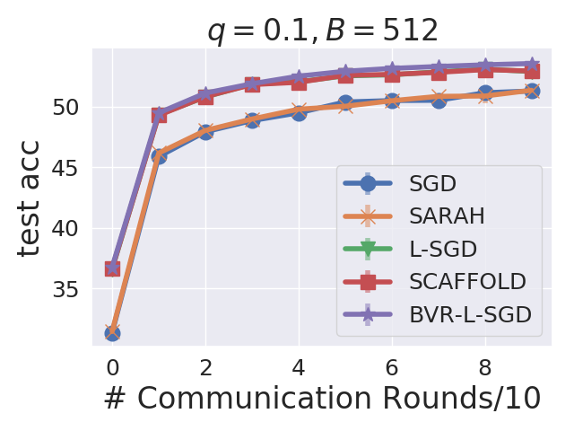
(d) Test Accuracy

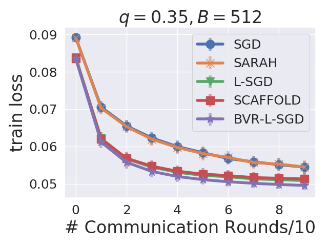
(e) Train Loss

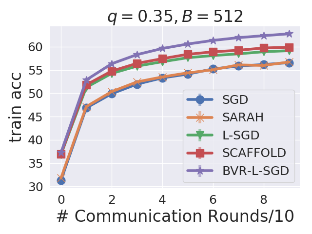
(f) Train Accuracy

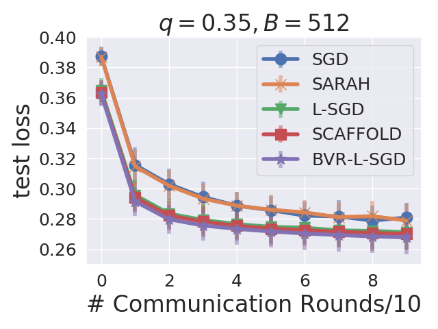
(g) Test Loss

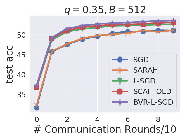
(h) Test Accuracy

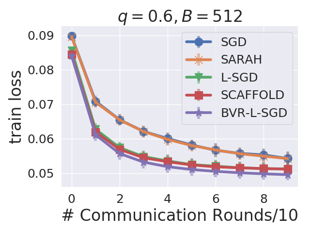
(i) Train Loss

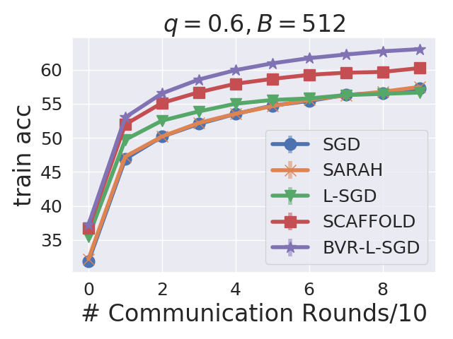
(j) Train Accuracy

(k) Test Loss

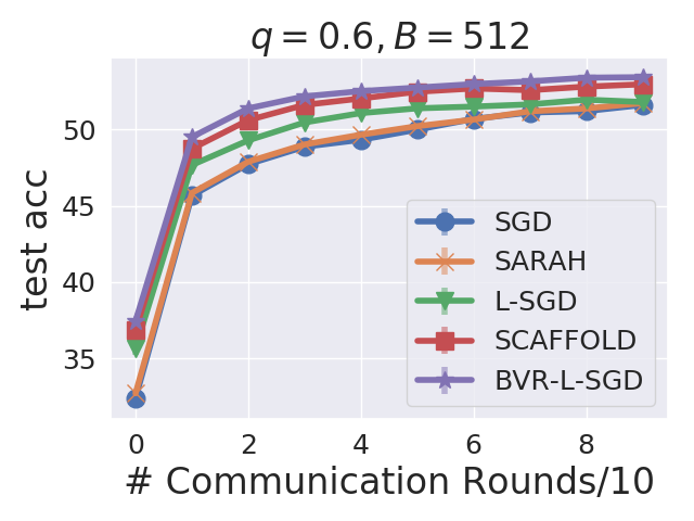
(l) Test Accuracy

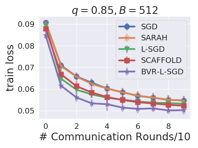
(m) Train Loss

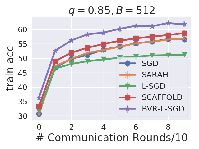
(n) Train Accuracy

(o) Test Loss

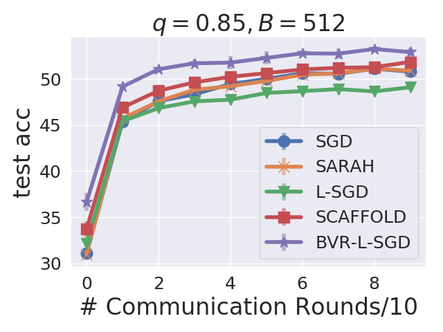
(p) Test Accuracy

Figure 6: Comparison of the train loss and test accuracy against the number of communication rounds for local computation budget $\mathcal{B}=512$.

4 4 4 4

(a) Train Loss

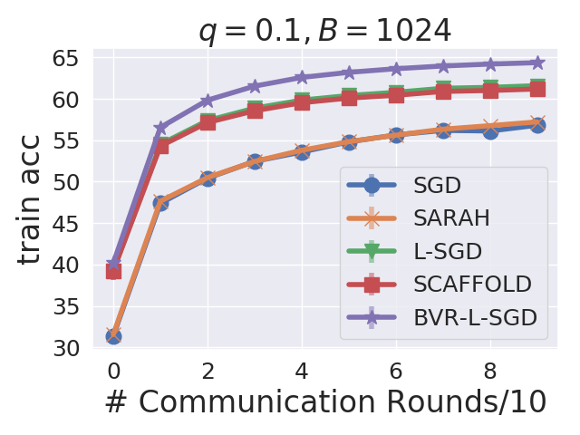
(b) Train Accuracy

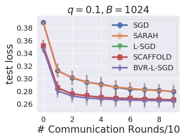
(c) Test Loss

(d) Test Accuracy

(e) Train Loss

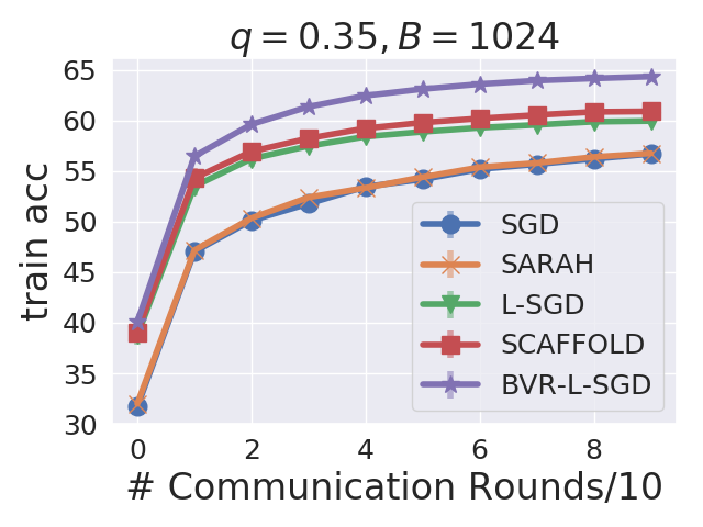
(f) Train Accuracy

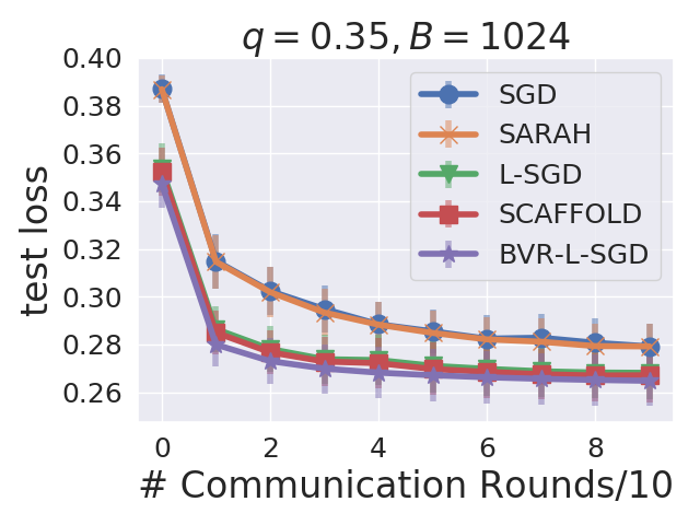
(g) Test Loss

(h) Test Accuracy

(i) Train Loss

(j) Train Accuracy

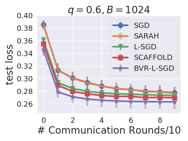
(k) Test Loss

(l) Test Accuracy

(m) Train Loss

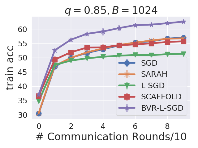
(n) Train Accuracy

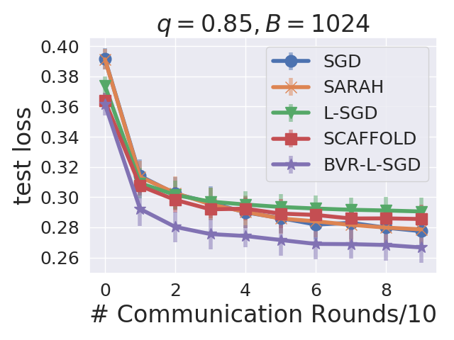
(o) Test Loss

(p) Test Accuracy

Figure 7: Comparison of the train loss and test accuracy against the number of communication rounds for local computation budget $\mathcal{B}=1,024$.

Computing Infrastructures

• OS: Ubuntu 16.04.6

• CPU: Intel(R) Xeon(R) CPU E5-2680 v4 @ 2.40GHz

• CPU Memory: 128 GB.

• GPU: NVIDIA Tesla P100.

• GPU Memory: 16 GB

• Programming language: Python 3.7.3.

• Deep learning framework: Pytorch 1.3.1.

References

- Allen-Zhu (2017) Allen-Zhu, Z. Natasha 2: Faster non-convex optimization than sgd. arXiv preprint arXiv:1708.08694, 2017.
- Allen-Zhu & Hazan (2016) Allen-Zhu, Z. and Hazan, E. Variance reduction for faster non-convex optimization. In International conference on machine learning, pp. 699–707. PMLR, 2016.
- Das et al. (2020) Das, R., Acharya, A., Hashemi, A., Sanghavi, S., Dhillon, I. S., and Topcu, U. Faster non-convex federated learning via global and local momentum. arXiv preprint arXiv:2012.04061, 2020.
- Dekel et al. (2012) Dekel, O., Gilad-Bachrach, R., Shamir, O., and Xiao, L. Optimal distributed online prediction using mini-batches. Journal of Machine Learning Research, 13(1), 2012.
- Fang et al. (2018) Fang, C., Li, C. J., Lin, Z., and Zhang, T. Spider: Near-optimal non-convex optimization via stochastic path integrated differential estimator. arXiv preprint arXiv:1807.01695, 2018.
- Ge et al. (2015) Ge, R., Huang, F., Jin, C., and Yuan, Y. Escaping from saddle points—online stochastic gradient for tensor decomposition. In Conference on learning theory, pp. 797–842. PMLR, 2015.
- Glorot & Bengio (2010) Glorot, X. and Bengio, Y. Understanding the difficulty of training deep feedforward neural networks. In Proceedings of the thirteenth international conference on artificial intelligence and statistics, pp. 249–256. JMLR Workshop and Conference Proceedings, 2010.
- Goyal et al. (2017) Goyal, P., Dollár, P., Girshick, R., Noordhuis, P., Wesolowski, L., Kyrola, A., Tulloch, A., Jia, Y., and He, K. Accurate, large minibatch sgd: Training imagenet in 1 hour. arXiv preprint arXiv:1706.02677, 2017.
- Haddadpour & Mahdavi (2019) Haddadpour, F. and Mahdavi, M. On the convergence of local descent methods in federated learning. arXiv preprint arXiv:1910.14425, 2019.
- Haddadpour et al. (2019) Haddadpour, F., Kamani, M. M., Mahdavi, M., and Cadambe, V. R. Local sgd with periodic averaging: Tighter analysis and adaptive synchronization. arXiv preprint arXiv:1910.13598, 2019.
- Jin et al. (2017) Jin, C., Ge, R., Netrapalli, P., Kakade, S. M., and Jordan, M. I. How to escape saddle points efficiently. In International Conference on Machine Learning, pp. 1724–1732. PMLR, 2017.
- Johnson & Zhang (2013) Johnson, R. and Zhang, T. Accelerating stochastic gradient descent using predictive variance reduction. Advances in neural information processing systems, 26:315–323, 2013.
- Kairouz et al. (2019) Kairouz, P., McMahan, H. B., Avent, B., Bellet, A., Bennis, M., Bhagoji, A. N., Bonawitz, K., Charles, Z., Cormode, G., Cummings, R., et al. Advances and open problems in federated learning. arXiv preprint arXiv:1912.04977, 2019.
- Karimireddy et al. (2020a) Karimireddy, S. P., Jaggi, M., Kale, S., Mohri, M., Reddi, S. J., Stich, S. U., and Suresh, A. T. Mime: Mimicking centralized stochastic algorithms in federated learning. arXiv preprint arXiv:2008.03606, 2020a.
- Karimireddy et al. (2020b) Karimireddy, S. P., Kale, S., Mohri, M., Reddi, S., Stich, S., and Suresh, A. T. Scaffold: Stochastic controlled averaging for federated learning. In International Conference on Machine Learning, pp. 5132–5143. PMLR, 2020b.
- Khaled et al. (2020) Khaled, A., Mishchenko, K., and Richtárik, P. Tighter theory for local sgd on identical and heterogeneous data. In International Conference on Artificial Intelligence and Statistics, pp. 4519–4529. PMLR, 2020.
- Koloskova et al. (2020) Koloskova, A., Loizou, N., Boreiri, S., Jaggi, M., and Stich, S. A unified theory of decentralized sgd with changing topology and local updates. In International Conference on Machine Learning, pp. 5381–5393. PMLR, 2020.
- Konečnỳ et al. (2015) Konečnỳ, J., McMahan, B., and Ramage, D. Federated optimization: Distributed optimization beyond the datacenter. arXiv preprint arXiv:1511.03575, 2015.
- Lei et al. (2017) Lei, L., Ju, C., Chen, J., and Jordan, M. I. Non-convex finite-sum optimization via scsg methods. arXiv preprint arXiv:1706.09156, 2017.
- Li (2019) Li, Z. Ssrgd: Simple stochastic recursive gradient descent for escaping saddle points. arXiv preprint arXiv:1904.09265, 2019.
- Lin et al. (2018) Lin, T., Stich, S. U., Patel, K. K., and Jaggi, M. Don’t use large mini-batches, use local sgd. arXiv preprint arXiv:1808.07217, 2018.
- McMahan et al. (2017) McMahan, B., Moore, E., Ramage, D., Hampson, S., and y Arcas, B. A. Communication-efficient learning of deep networks from decentralized data. In Artificial Intelligence and Statistics, pp. 1273–1282. PMLR, 2017.
- Nguyen et al. (2017) Nguyen, L. M., Liu, J., Scheinberg, K., and Takáč, M. Sarah: A novel method for machine learning problems using stochastic recursive gradient. In International Conference on Machine Learning, pp. 2613–2621. PMLR, 2017.
- Nguyen et al. (2019) Nguyen, L. M., van Dijk, M., Phan, D. T., Nguyen, P. H., Weng, T.-W., and Kalagnanam, J. R. Finite-sum smooth optimization with sarah. arXiv preprint arXiv:1901.07648, 2019.
- Reddi et al. (2016a) Reddi, S. J., Hefny, A., Sra, S., Poczos, B., and Smola, A. Stochastic variance reduction for nonconvex optimization. In International conference on machine learning, pp. 314–323. PMLR, 2016a.
- Reddi et al. (2016b) Reddi, S. J., Konečnỳ, J., Richtárik, P., Póczós, B., and Smola, A. Aide: Fast and communication efficient distributed optimization. arXiv preprint arXiv:1608.06879, 2016b.
- Sharma et al. (2019) Sharma, P., Kafle, S., Khanduri, P., Bulusu, S., Rajawat, K., and Varshney, P. K. Parallel restarted spider–communication efficient distributed nonconvex optimization with optimal computation complexity. arXiv preprint arXiv:1912.06036, 2019.
- Shokri & Shmatikov (2015) Shokri, R. and Shmatikov, V. Privacy-preserving deep learning. In Proceedings of the 22nd ACM SIGSAC conference on computer and communications security, pp. 1310–1321, 2015.
- Stich (2018) Stich, S. U. Local sgd converges fast and communicates little. arXiv preprint arXiv:1805.09767, 2018.
- Woodworth et al. (2020a) Woodworth, B., Patel, K. K., and Srebro, N. Minibatch vs local sgd for heterogeneous distributed learning. arXiv preprint arXiv:2006.04735, 2020a.
- Woodworth et al. (2020b) Woodworth, B., Patel, K. K., Stich, S., Dai, Z., Bullins, B., Mcmahan, B., Shamir, O., and Srebro, N. Is local sgd better than minibatch sgd? In International Conference on Machine Learning, pp. 10334–10343. PMLR, 2020b.
- Yu et al. (2019) Yu, H., Yang, S., and Zhu, S. Parallel restarted sgd with faster convergence and less communication: Demystifying why model averaging works for deep learning. In Proceedings of the AAAI Conference on Artificial Intelligence, volume 33, pp. 5693–5700, 2019.
- Zhou et al. (2018) Zhou, D., Xu, P., and Gu, Q. Stochastic nested variance reduction for nonconvex optimization. arXiv preprint arXiv:1806.07811, 2018.