Probing the structure of the $B$ meson with $B\to\ell\ell\ell^{\prime}\nu$

Abstract

We consider the decay $B\to\ell\ell\ell^{\prime}\nu$, taking into account the leading $1/m_{b}$ and $q^{2}$ corrections calculated in the QCD factorization framework as well as the soft corrections calculated employing dispersion relations and quark-hadron duality. We extend the existing results for the radiative decay $B\to\gamma\ell\nu$ to the case of non-zero (but small) $q^{2}$, the invariant mass squared of the dilepton pair $\ell^{+}\ell^{-}$. This restricts us to the case $\ell\neq\ell^{\prime}$ as otherwise the same sign $\ell$ and $\ell^{\prime}$ cannot be distinguished. We further study the sensitivity of the results to the leading moment of the $B$-meson distribution amplitude and discuss the potential to extract this quantity at LHCb and the Belle II experiment.

1 Introduction

Our understanding of the structure of the $B$ meson lacks the precision needed to provide accurate predictions of $B$-meson decays beyond naive factorization. The quantity most vitally required for making these predictions, whether using QCD factorization or light-cone sum rules (LCSR), is the leading moment of the $B$-meson distribution amplitude, $\lambda_{B}$, defined by (see e.g. Ref. [1])

$$\lambda_{B}^{-1}(\mu)=\int_{0}^{\infty}\frac{dk}{k}\phi_{B}^{+}(k,\mu),$$ (1)

where $\phi_{B}^{+}(k,\mu)$ is the distribution amplitude of the $B$ meson, depending on the scale $\mu$. The theoretical uncertainty on $\lambda_{B}$ is large with estimates ranging from $200$ MeV obtained using non-leptonic decays [2, 3] to $460\pm 110$ MeV obtained from QCD sum rules [1].

It was proposed in Refs. [4, 5, 6] to use the charged current decay of the $B^{+}$ meson, with an extra photon in the final state i.e., $B^{+}\to\ell^{+}\nu\gamma$ to probe $\lambda_{B}$ in the kinematic limit when the energy of the photon is large in comparison to the scale of strong interactions ($\Lambda_{\rm QCD}$). Note that the branching ratio is larger than for the purely leptonic final state, as the emission of the photon lifts the helicity suppression. On the experimental side, the most stringent limit from the BaBar collaboration was [7]

$$\mathcal{BR}(B^{+}\to\ell^{+}\nu\gamma)<15.6\times 10^{-6},$$ (2)

at $90\%$ confidence level (C.L.), resulting in the lower limit $\lambda_{B}>300$ MeV [7]. The Belle collaboration has provided an upper limit on the branching ratios for the electron and muon final states [8]:

$$\mathcal{BR}(B^{+}\to e^{+}\nu\gamma) <4.3\times 10^{-6},$$ (3)

$$\mathcal{BR}(B^{+}\to\mu^{+}\nu\gamma) <3.4\times 10^{-6},$$ (4)

also at $90\%$ C.L., providing a lower limit of $\lambda_{B}>238$ MeV. Note that the fact that the Belle lower limit lies below the BaBar limit, despite the limit on the branching ratio being more stringent, is due to both to a different choice of input parameters (particularly $m_{b}$ and $|V_{ub}|$) and the fact that in Ref. [8] the expression for the partial branching fraction include state-of-the-art next-to-leading order corrections from Ref. [9] and the soft corrections calculated in Ref. [10].

Updating this result is a priority at Belle II, and projections look very promising [11, 12]. However, the measurement of $B\to\gamma\ell\nu$ at LHCb is challenging as the low energy photon in combination with the neutrino in the final state provide complications for the trigger. On the other hand, if the photon was off-shell and emitted a lepton pair, then for the final state consisting of three charged leptons and a neutrino the analysis would be feasible. In fact, an upper limit at 95% C.L. has already been provided by LHCb in the region where the lowest of the muon pair mass combination is below $980$ MeV [13],

$$\mathcal{BR}(B^{+}\to\mu^{+}\mu^{-}\mu^{+}\nu)<1.6\times 10^{-8}.$$ (5)

In light of this measurement, it is of interest to assess whether $B\to\ell\ell\ell^{\prime}\nu$ could be a source of complementary information about the nature of the $B$-meson distribution amplitude. On the theoretical side the extension of the full existing formalism for $B\to\gamma\ell\nu$ to this case has not yet been attempted, although a first prediction of the branching ratio can be found in Ref. [14, 15], based on the vector meson dominance approach. Here the branching ratio was predicted to be $\sim 3\times 10^{-7}$ (above the experimental limit from LHCb) without an analysis of the associated uncertainties.

Our aim is therefore to provide predictions for the differential decay spectrum and the partial branching fraction for $B\to\ell\ell\ell^{\prime}\nu$, which, with more data, could lead to the measurement of the first moment of the $B$-meson distribution amplitude at LHCb. This would serve as an important cross-check for the results from Belle II. Here it is important to note that the framework in which our calculation is performed means that the results are only valid at low $q^{2}$, where $q^{2}$ is the dilepton mass squared for the $\ell^{+}\ell^{-}$ pair originating from the virtual photon. Since when $\ell=\ell^{\prime}$, this theoretical definition of $q^{2}$ cannot be measured experimentally, due to the ambiguity between the same sign leptons, such that the existing limit from LHCb cannot be converted into a lower limit on $\lambda_{B}$. We will therefore concentrate on the case $\ell\neq\ell^{\prime}$.

In the following section we will introduce our theoretical framework, expressing the amplitude for the decay in terms of the form factors, and providing details of the various contributions to these form factors that we include. In Sec. 3, after having discussed the kinematics necessary to calculate the branching ratio and the parameters adopted, we will present the results of our numerical analysis. Finally, a discussion of these results and our conclusions can be found in Sec. 4.

2 Theoretical framework

2.1 The Effective Amplitude

The amplitude for the process $B^{+}(p_{B})\to\ell^{+}(q_{1})\ell^{-}(q_{2})\ell^{\prime+}(p_{1}){\nu}(p_{2})$ can be written as

$$iA=\frac{G_{F}V_{ub}}{\sqrt{2}}\frac{ie^{2}}{q^{2}}(\bar{u}_{\ell}\gamma^{\mu}v_{\ell})[(\bar{u}_{\nu}\gamma^{\rho}P_{L}v_{\ell^{\prime}})T_{\mu\rho}-i(\bar{u}_{\nu}\gamma_{\mu}P_{L}v_{\ell^{\prime}})f_{B}]$$ (6)

where $G_{F}$ is the Fermi constant, $V_{ub}$ is the CKM matrix element and $e$ is the electric charge. Here the first term describes the emission of the virtual photon from the $B$ meson and the second term from the lepton. At leading order the second term can trivially be written in terms of the $B$-meson decay constant $f_{B}$, whereas the first term is more complicated and requires further study. On writing down this term in the most general form as possible, imposing the conservation of the electromagnetic current and applying the equation of motion (see Appendix A), the tensor $T_{\mu\rho}$ defined in Eq. (6) reduces to,

$$T_{\mu\rho}=iF_{A}(g_{\mu\rho}(p\cdot q)-p_{\mu}q_{\rho})+F_{V}\epsilon_{\rho\mu\lambda\sigma}p^{\lambda}q^{\sigma},$$ (7)

where $p=p_{1}+p_{2}$ and $q=q_{1}+q_{2}$. Therefore this contribution to the decay amplitude can be expressed in terms of two form factors $F_{V}$ and $F_{A}$, as in the case of $B\to\gamma\ell\nu$. The amplitude can then be expressed as

$${}iA=\frac{G_{F}V_{ub}}{\sqrt{2}}\frac{ie^{2}}{q^{2}}(\bar{\ell}\gamma^{\mu}\ell)(\bar{\nu}\Gamma^{\rho}\ell^{\prime})\Big{[}iF_{A}(g_{\mu\rho}\,p.q-p_{\mu}q_{\rho})+F_{V}\,\epsilon_{\rho\mu\lambda\sigma}\,p^{\lambda}q^{\sigma}\Big{]},$$ (8)

Making predictions for these decays therefore comes down to obtaining expressions for these form factors. Note that the mass of the leptons in the final state has been neglected, which results in the exact cancellation of the contact term with the contribution of photon emission from charged lepton. However, in case of tau leptons in the final state, additional form factors may appear and would need to be calculated.

2.2 Form Factors

The form factors defined in Eq. (7) are functions of $q^{2}$. They have been calculated for the case $B\to\gamma\ell\nu$ (i.e. $q^{2}=0$) and therefore these results need to be extended. We will therefore first review the results for $q^{2}=0$, before presenting our calculation at non-zero $q^{2}$.

2.2.1 State-of-the-art result for $B\to\gamma\ell\nu$

In the case of $B\to\gamma\ell\nu$, from Ref. [16] we have

$$F_{V}= \frac{Q_{u}\,f_{B}\,m_{B}}{2\,E_{\gamma}\,\lambda_{B}(\mu)}R(E_{\gamma}\,\mu)+\xi(E_{\gamma})+\Delta\xi(E_{\gamma})$$

$$F_{A}= \frac{Q_{u}\,f_{B}\,m_{B}}{2\,E_{\gamma}\,\lambda_{B}(\mu)}R(E_{\gamma},\mu)+\xi(E_{\gamma})-\Delta\xi(E_{\gamma}),$$ (9)

where the photon energy $E_{\gamma}=(m_{B}^{2}-p^{2})/(2m_{B})$, $Q_{u}$ is the charge of the $u$ quark and $m_{B}$ is the mass of the $B$ meson. The first term is the leading contribution in the heavy quark expansion, which depends inversely on the quantity of interest, $\lambda_{B}$, the first inverse moment of the $B$-meson distribution amplitude defined in Eq. (1). Note here that the factor $R(E_{\gamma},\mu)$ contains the radiative corrections calculated in Ref. [9], and at tree level is equal to 1. The second term encodes the symmetry conserving soft and $\mathcal{O}(1/m_{b},1/E_{\gamma})$ corrections to the form factors which may be sizeable. The soft corrections, arising when the quark propagator between the electromagnetic and weak vertices becomes soft, have been calculated making use of dispersion relations and quark-hadron duality, up to next-to-leading order (NLO) at leading twist and up to twist-6 at leading order [16, 17, 18]. The last term contains the symmetry breaking corrections, which arise at $\mathcal{O}(1/m_{b},1/E_{\gamma})$ in QCD factorization, as well as receiving contributions from the soft corrections at twist-3 to 6 [17, 18, 16].

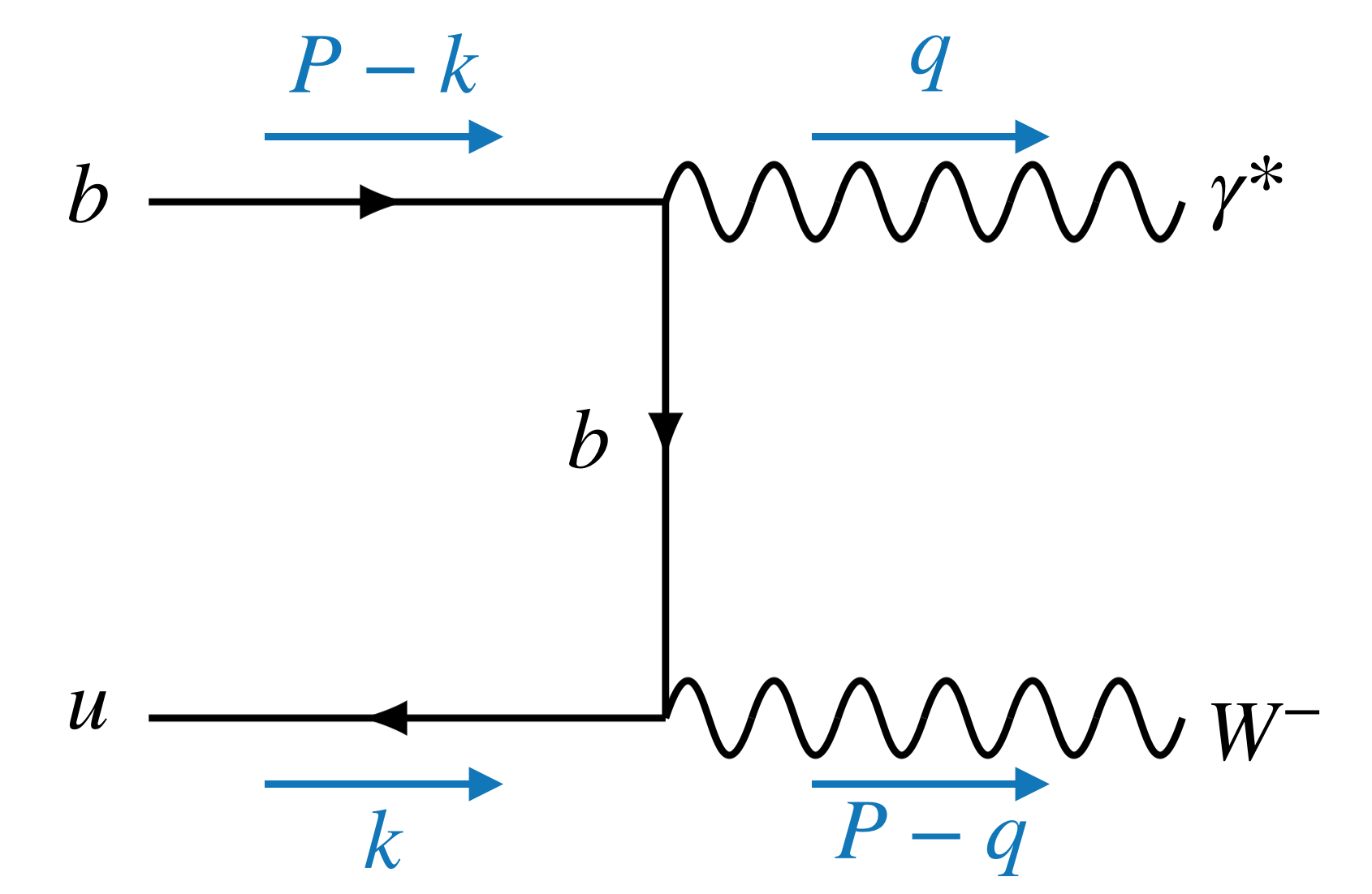
Figure 1: (a): photon emission from u quark, (b): photon emission from $b$ quark

2.2.2 Symmetric corrections for $B\to\ell\ell\ell^{\prime}\nu$ at leading order in $\alpha_{s}$

We now wish to extend these calculations to the case of non-zero $q^{2}$. In $B\to\gamma\ell\nu$, factorization holds as long as the photon is energetic in the rest frame of the $B$ meson, implying that the photon energy is $\sim m_{b}$. Similarly in our case a hard collinear virtual photon coupling to the spectator $u$ quark can be integrated out systematically, and the total amplitude is found to be factorized into a hard scattering kernel and a soft part, given by the distribution amplitude. In the same setting, the resulting contribution from the $b$ quark is found to be power suppressed. A quick analysis of the diagrams for the case of a soft emitted photon reveals that there are possibly power enhanced contributions, coming both from the $u$-quark and $b$-quark legs. However, these are not expected to be factorizable and will not be considered any further. We thus restrict our attention to the case of a hard collinear photon (defined below) for which the factorization is found to hold, constraining $q^{2}$ to be not too far from zero. Thus at the leading order, only the left-hand diagram in Fig. 1 contributes to the form factors.

For convenience, we choose to work in light-cone coordinates ($l\equiv(l_{+},l_{-},l_{\perp})$) where,

$$l_{\pm}=\frac{l_{0}\pm l_{3}}{2}, l_{\perp}=(l_{1},l_{2}).$$ (10)

As the spectator quark is soft, its momentum will scale as $k=(k_{+},k_{-},k_{\perp})\sim(\lambda,\lambda,\lambda)$, while the momentum of the virtual photon scales as $q=(q_{+},q_{-},q_{\perp})\sim(\lambda,1,\lambda^{1/2})$. This implies that,

$$(q-k)^{2}\sim q^{2}-2q_{-}k_{+}\ldots$$ (11)

where we neglect terms that are suppressed by higher powers of $\lambda$, such that the propagator can be expressed as

$$\frac{\not{q}-\not{k}}{(q-k)^{2}}=\frac{q_{-}\not{n}_{+}}{q^{2}-2q_{-}k_{+}}-\left(\frac{k_{+}\not{n}_{-}}{q^{2}-2q_{-}k_{+}}+\frac{k_{-}\not{n}_{+}}{q^{2}-2q_{-}k_{+}}+\frac{\not{k}_{\perp}}{q^{2}-2q_{-}k_{+}}\right).$$ (12)

Here the first term provides the leading contribution and the terms in brackets are suppressed by $\lambda$. Expressing the four-momentum of the virtual photon as $q^{\mu}=(E,q_{\perp},-q_{3})$, the components in light-cone coordinates, $(q_{+},q_{-},q_{\perp})$, can be expressed as

$$q_{+} =\frac{1}{2}(E-q_{3}) q_{-}=\frac{1}{2}(E+q_{3}).$$ (13)

When the photon is hard-collinear, $q_{-}\sim E$ at leading order. Thus, $2q_{-}k_{+}\simeq 2E\,k_{+}+\mathcal{O}(1/E)$. Using this and following Ref. [10], the form factor at leading order in the heavy quark and the perturbative expansion, arising from the first term in Eq. (12), reads,

$$F_{B\to\gamma^{\ast}}(q^{2},p^{2})=Q_{u}f_{B}\int_{0}^{\infty}dk_{+}\frac{\phi_{B}^{+}(k_{+})}{2E\,k_{+}-q^{2}-i\epsilon}.$$ (14)

We now wish to include the soft contribution, i.e. the non-perturbative contribution to the form factors which is not accesible via QCD factorization, calculated using dispersion relations and quark-hadron duality in Ref. [1, 16] using a technique similar to one applied to the $\gamma^{*}\gamma\pi$ form factor [19]. The idea is to relate via a dispersion relation the form factor at the desired $q^{2}$ to that at $q^{2}=-m_{B}\Lambda_{\rm QCD}$, where the result can easily be calculated perturbatively to arbitrary precision in the expansion in $1/m_{b}$, $q^{2}$, $1/E$. This requires an assumption to be made about the hadronic spectral density as a function of $q^{2}$. Following Refs. [10, 16], one easily obtains the result for the two form factors $F_{V}$ and $F_{A}$ at leading order in the twist and perturbative expansion,

$$F^{\mathrm{sym}}_{V/A}= \,Q_{u}f_{B}\bigg{(}\int_{\tfrac{s_{0}}{2E}}^{\infty}dk_{+}\frac{\phi_{B}^{+}(k_{+})}{2E\,k_{+}-q^{2}-i\epsilon}$$

$$\qquad\qquad\qquad+\int_{0}^{\tfrac{s_{0}}{2E}}dk_{+}\frac{e^{-(2Ek_{+}-m_{\rho}^{2})/M^{2}}}{m_{\rho}^{2}-q^{2}-i\epsilon}\phi_{B}^{+}(k_{+})\bigg{)}.$$ (15)

where $s_{0}$ is the continuum threshold, $m_{\rho}$ is the mass of $\rho$ meson, and $M$ is the Borel parameter. Note that $s_{0}$ corresponds to the value of $q^{2}$ above which quark-hadron duality is expected to hold. The Borel parameter enters the result due to fact that a Borel transformation has been performed in order to reduce the sensitivity to this assumption. Note that here, on comparing Eqs. (14) and (2.2.2) the soft contribution at leading order to the form factor can be extracted,

$$\xi_{\rm soft}=\,Q_{u}f_{B}\int_{0}^{\tfrac{s_{0}}{2E}}dk_{+}\left(\frac{e^{-(2Ek_{+}-m_{\rho}^{2})/M^{2}}}{m_{\rho}^{2}-q^{2}-i\epsilon}-\frac{1}{2E\,k_{+}-q^{2}-i\epsilon}\right)\phi_{B}^{+}(k_{+}).$$ (16)

2.2.3 Symmetric corrections for $B\to\ell\ell\ell^{\prime}\nu$ at NLL

Comparing Eq. (2.2.2) to Eq. (9) we observe two differences. The first is that $q^{2}$ now appears in the denominator. The second is that we have not yet included the factor $R(E_{\gamma},\mu)$ containing the NLL corrections. The radiative corrections for $B\to\ell\nu\gamma$ at NLL are significant and were seen in Refs. [9, 16] to affect the form factors by $20-40\%$. Note that these NLL corrections not only affect the leading-order contribution, i.e. the first term in Eq. (9), but also the soft contribution, as described in Ref. [16]. The factor $R(E_{\gamma},\mu)$ introduced in Ref.  via [9] can be adapted to our case,

$$R(p^{2},q^{2},\mu)=C(p^{2},q^{2},\mu_{h1})K^{-1}(\mu_{h2})U(p^{2},q^{2},\mu_{h1},\mu_{h2},\mu)J(p^{2},q^{2},\mu).$$ (17)

Here $C(p^{2},q^{2},\mu_{h1})$ is obtained from matching the QCD heavy-to-light current to the corresponding SCET current at the hard scale $\mu_{h1}$. The result at NLO was calculated in Ref. [20, 6, 21] and can also be found in Ref. [9], and is applicable for both $B\to\gamma\ell\nu$ and $B\to\ell\ell\ell^{\prime}\nu$. The same goes for the factor $K(\mu_{h2})$, which accounts for the conversion from the static $B$-meson decay constant in the SCET current to the standard definition in QCD, $f_{B}$, used in our analysis, more details and the expression can be found in Ref. [9]. Letting aside momentarily the renormalization group evolution (RGE) factor $U(p^{2},q^{2},\mu_{h1},\mu_{h2},\mu)$, let us first discuss the factor $J(p^{2},q^{2},\mu)$. This accounts for the hard-collinear radiative corrections, and was calculated for $B\to\gamma\ell\nu$ in Refs [20, 6]. For $B\to\ell\ell\ell^{\prime}\nu$ where $q^{2}\neq 0$ we can adopt the expression given in Ref. [17].

Returning to the RGE factor $U(p^{2},q^{2},\mu_{h1},\mu_{h2},\mu)$, we see that for any choice of the scales $\mu_{h1}$, $\mu_{h2}$ and $\mu$, some large logarithms arising in the expressions for $C(p^{2},q^{2},\mu_{h1})$, $K(\mu_{h2})$ and $J(p^{2},q^{2},\mu)$ will remain. Therefore it makes sense to resum these logarithms to all orders by solving a renormalization group equation [6]. This resummation results in the factor $U(p^{2},q^{2},\mu_{h1},\mu_{h2},\mu)$, which can be found in Ref. [9]. This factor depends on three scales: the hard scales $\mu_{h1}$ and $\mu_{h2}$ are taken to be $2E$ and $m_{b}$ respectively, while the hard-collinear scale $\mu$ is set to $(m_{b}\Lambda_{\rm QCD})^{1/2}$.

Putting this together we find the result at leading order in the heavy quark expansion, and NLL in the perturbative expansion to be

$$F_{V/A}^{\rm NLL}= \,\frac{Q_{u}\,m_{B}f_{B}}{2E\,\lambda_{B}}C(p^{2},q^{2},\mu_{h1})K^{-1}(\mu_{h2})U(p^{2},q^{2},\mu_{h1},\mu_{h2},\mu)\,J(p^{2},q^{2},\mu),$$ (18)

where we remind the reader that these are symmetric contributions. As mentioned earlier, including these NLL corrections has the consequence that the expression for soft contribution to the form factors given in Eq. (2.2.2) is no longer valid. This can be understood in terms of the following relation [9],

$$\xi_{\rm soft}=\frac{1}{\pi}\int_{0}^{s_{0}}\mathrm{d}s\left(\frac{e^{-(s-m_{\rho}^{2})/M^{2}}}{m_{\rho}^{2}-q^{2}-i\varepsilon}-\frac{1}{s-q^{2}-i\varepsilon}\right){\rm Im}F^{\rm QCD}(E,s).$$ (19)

Adopting $F^{\rm QCD}(E,s)=F^{\rm NLL}_{V/A}$ from Eq. (18), setting $\omega^{\prime}=s/(2E)$, and with the help of Appendix A of Ref. [17] we therefore obtain

$$\xi_{\rm soft}^{\rm NLL}=\, \,Q_{u}m_{B}f_{B}C(p^{2},q^{2},\mu_{h1})K^{-1}(\mu_{h2})U(p^{2},q^{2},\mu_{h1},\mu_{h2},\mu)$$

$$\int_{0}^{\tfrac{s_{0}}{2E}}\mathrm{d}\omega^{\prime}\left(\frac{e^{-(2E\,\omega^{\prime}-m_{\rho}^{2})/M^{2}}}{m_{\rho}^{2}-q^{2}-i\varepsilon}-\frac{1}{2E\,\omega^{\prime}-q^{2}-i\varepsilon}\right)\phi_{+}^{\rm eff}(\omega^{\prime},\mu)$$ (20)

where an expression for $\phi_{+}^{\rm eff}(\omega^{\prime},\mu)$ can be found in Ref. [16]. Note that, as was observed in Ref. [16] for the radiative mode, we find that on including NLL contributions the separation between the hard and soft parts, $F_{V/A}^{\rm NLL}$ and $\xi_{\rm soft}^{\rm NLL}$ respectively, becomes complicated, and henceforth we will consider the finite quantity

$$F_{V/A}^{\rm NLL}+\xi_{\rm soft}^{\rm NLL}=\, \,Q_{u}m_{B}f_{B}C(p^{2},q^{2},\mu_{h1})K^{-1}(\mu_{h2})U(p^{2},q^{2},\mu_{h1},\mu_{h2},\mu)$$

$$\left(\int_{0}^{\tfrac{s_{0}}{2E}}\mathrm{d}\omega^{\prime}\frac{e^{-(2E\,\omega^{\prime}-m_{\rho}^{2})/M^{2}}}{m_{\rho}^{2}-q^{2}-i\varepsilon}\phi_{+}^{\rm eff}(\omega^{\prime},\mu)-\int_{\tfrac{s_{0}}{2E}}^{\infty}\mathrm{d}\omega^{\prime}\frac{\phi_{+}^{\rm eff}(\omega^{\prime},\mu)}{2E\,\omega^{\prime}-q^{2}-i\varepsilon}\right).$$ (21)

2.2.4 Symmetry-breaking corrections

Having obtained the expression for the symmetry-conserving contributions to the form factors, we now consider the symmetry-breaking correction terms. Considering the leading power suppressed term in the $u$-quark propagator, we find

$$\Delta F_{V}^{(u)}=-\Delta F_{A}^{(u)}=\, \,Q_{u}\,f_{B}\,\int_{0}^{\infty}dk_{+}\phi_{B}^{+}\frac{1}{4E^{2}}\left(\frac{q^{2}}{2E\,k_{+}-q^{2}}+1\right)$$

$$=\, \,\frac{1}{4E^{2}}\left(Q_{u}f_{B}+q^{2}\,F^{\mathrm{sym}}_{V/A}\right)$$ (22)

The contribution arising due to the virtual photon emission from the $b$-quark leg is also power suppressed and has been neglected while computing the symmetry preserving, leading order contribution to the form factors. Similar to the $u$-quark contribution, the emission from the $b$-quark leg yields symmetry breaking correction which is conveniently written as

$$\Delta F_{V}^{(b)}=-\Delta F_{A}^{(b)}=\, \,Q_{b}f_{B}\int_{0}^{\infty}dk_{+}\phi_{B}^{+}\frac{1}{2m_{b}E}\left(\frac{q^{2}}{2E\,k_{+}-q^{2}}+1\right)$$

$$=\, \,\frac{Q_{b}}{2m_{b}E}\left(f_{B}+\frac{q^{2}}{Q_{u}}\,F^{\mathrm{sym}}_{V/A}\right)$$ (23)

2.2.5 Summary of contributions to the form factors

Combining Eqs. (21), (2.2.4) and (2.2.4), we obtain the final results for our form factors for the decay $B\to\ell\ell\ell^{\prime}\nu$,

$$F_{V}= F_{V}^{\rm NLL}+\xi_{\rm soft}^{\rm NLL}+\Delta F_{V}^{(u)}+\Delta F_{V}^{(b)}$$

$$F_{A}= F_{A}^{\rm NLL}+\xi_{\rm soft}^{\rm NLL}+\Delta F_{A}^{(u)}+\Delta F_{A}^{(b)},$$ (24)

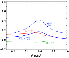
Figure 2: Different contributions to form factors are shown as a function of $q^{2}$ at a fixed value of $p^{2}=10$ GeV². The dotted (solid) blue curve shows the symmetric leading order (NLL) contribution $F_{V/A}^{\rm sym}$ ($F_{V/A}^{\rm NLL}+\xi_{\rm soft}^{\rm NLL}$). The red and green dotted curves show the symmetry breaking contributions of $u$ quark ($\Delta{F}_{V}^{(u)}$) and $b$ quark ($\Delta{F}_{V}^{(b)}$) respectively, scaled by a factor of 10.

In order to compare the different contributions to the form factors we plot the individual terms as a function of $q^{2}$ in Fig. 2 for $p^{2}=10$ GeV². The dotted blue curve shows the form factors at leading order $F_{V/A}^{\rm sym}$, as defined in Eq. (2.2.2). The solid blue curve shows the form factors after including the radiative and soft corrections, i.e. $F_{V/A}^{\rm NLL}+\xi_{\rm soft}^{\rm NLL}$ as given in Eq. (21). Note that the contribution of the symmetry-breaking terms is at most $10\%$ of the symmetry-preserving terms, and therefore we have scaled them by a factor of 10 in the plot. The red and green dotted curves show these scaled symmetry breaking terms, $\Delta F_{V}^{(u)}$ from Eq. (2.2.4) and $\Delta F_{V}^{(b)}$ from Eq. (2.2.4) respectively. The contribution of photon emission from the $b$ quark is always negative due to the negative charge of the $b$ quark. In Fig. 2 we see that the contribution of $\Delta F_{V}^{(b)}$ is highly suppressed in comparison to $\Delta{F}_{V}^{(u)}$ near $q^{2}=1$ GeV² ($\Delta F_{V}^{(u)}(1\,\mbox{GeV}^{2})\sim 5\Delta{F}_{V}^{(b)}(1\,\mbox{GeV}^{2})$) but the two quantities are comparable at low $q^{2}$. We further observe that radiative corrections reduce the form factor at leading order by a factor of $30-60\%$, varying over the $q^{2}$ range.

The central values (for $\lambda_{B}=350$ MeV) of the symmetry-preserving and symmetry-breaking terms contributions to the form factors, as well as the uncertainty bands, are shown in Fig. 3. The input parameters and the related uncertainties used to calculate this uncertainty band are given in Table 1. On comparing the uncertainty due to the hard-collinear factorization scale $\mu$ and the total uncertainty, it is clear that the scale provides the dominant contribution to the uncertainty on the form factors. We further show $|F_{A}\pm F_{V}|/2$ for $\lambda_{B}=200$ and 500 MeV, and observe a strong dependence of the form factors on $\lambda_{B}$. This is in accordance with the results for the branching ratio, which will be discussed in detail in Sec. 3.

Note that there are several contributions which have been calculated in the state-of-the-art $B\to\gamma\ell\nu$ analysis which have been neglected here, namely the $\mathcal{O}(\alpha_{s})$ and the higher twist contributions. These contributions were seen to be relatively small, we will comment more on the uncertainty due to missing higher-twist and higher $\mathcal{O}(\alpha_{s})$ terms in the following section.

Parameter	Value	Ref.	Parameter	Value	Ref.
$m_{B}$	$5.28~{}\mathrm{GeV}$	[22]	$f_{B}$	$192.0\pm 4.3$ MeV	[22]
$\left|V_{ub}\right|^{\text{excl}}$	$(3.70\pm 0.16)\times 10^{-3}$	[22]	$G_{F}$	$1.166\times 10^{-5}~{}\mathrm{GeV}^{-2}$	[22]
$m_{\mu}$	$0.105~{}\mathrm{GeV}$	[22]	$\tau_{B}$	$(1.641\pm 0.008)\times 10^{-12}$ s	[22]
$M_{\rho}$	$0.775$ GeV	[22]	$m_{e}$	$0.511\times 10^{-3}~{}\mathrm{GeV}$	[22]
$\alpha_{em}$	$1/137$	[22]	$\lambda_{B}$	$[200-500]$ MeV	[16]
$s_{0}$	$1.5\pm 0.1$ GeV2	[16]	$M^{2}$	$1.25\pm 0.25$ GeV2	[16]

Table 1: Numerical values of parameters adopted in our analysis

3 Numerical analysis and results

In this section, we will first outline the kinematics required to describe the differential decay distribution of the four leptonic decay of charged $B$ meson. This will be followed by a discussion of the numerical parameters implemented in our analysis. We will then present the results, where numerical predictions for the decay process under study are provided in specific $q^{2}$ bins, along with a thorough analysis of the uncertainties.

3.1 Kinematics

We follow the definitions in [23] for the kinematics. In order to examine the partial decay rate of $B^{+}(p_{B})\to\ell^{+}(q_{1})\ell^{-}(q_{2})\ell^{\prime+}(p_{1})\nu(p_{2})$, it is useful to introduce the following combinations of the final state particles’ four-momenta:

$$q=q_{1}+q_{2}; Q=q_{1}-q_{2} p=p_{1}+p_{2} P=p_{1}-p_{2}.$$ (25)

This four-body partial decay rate can then be described via five independent variables:

• the effective mass squared, $p^{2}$ and $q^{2}$, of the $\ell^{\prime}\nu$ and $\ell^{+}\ell^{-}$ system respectively,

• the angles $\theta_{\gamma}$ of the $\ell^{+}$ in the $\ell^{+}\ell^{-}$ center-of-mass system with respect to the $\ell^{+}\ell^{-}$ line of flight in $B$ rest frame, and $\theta_{W}$ of the $\ell^{\prime}$ in the $\ell^{\prime}\nu$ center-of-mass system with respect to the $\ell^{\prime}\nu$ line of flight in $B$ rest frame, where

  $$\cos\,\theta_{\gamma}=-\frac{\vec{Q}~{}.~{}\vec{p}}{|\vec{Q}|~{}|\vec{p}|},\qquad\mbox{and}\qquad\cos\,\theta_{W}=-\frac{\vec{q}~{}.~{}\vec{P}}{|\vec{q}|~{}|\vec{P}|},$$ (26)

• the angle $\phi$ between the planes of the two lepton pairs,

  $$\sin\phi=\frac{(\vec{q}\times\vec{P})\times(\vec{p}\times\vec{Q})}{|\vec{q}\times\vec{P}|~{}|\vec{p}\times\vec{Q}|}.$$ (27)

In terms of these five variables, the partial decay distribution is given by,

$$d^{5}\Gamma=\frac{\pi\lambda(m_{B}^{2},q^{2},p^{2})^{1/2}}{(4\pi)^{7}}m_{B}^{5}|A|^{2}d\Phi$$ (28)

where $d\Phi$ denotes an element of the four-body phase space, and is defined via

$$d\Phi=dq^{2}~{}dp^{2}~{}d\cos\theta_{\gamma}~{}d\cos\theta_{W}~{}d\phi,$$ (29)

$A$ is the amplitude of the process defined in Eq. (8) and the Källén function is given by

$$\lambda(a,b,c)=a^{4}+b^{4}+c^{4}-2(a^{2}b^{2}+b^{2}c^{2}+c^{2}a^{2}).$$ (30)

Note that the decay distribution in Eq. (28) corresponds to the case when $\ell\neq\ell^{\prime}$. If the leptons in the final state are all of the same flavour, there is an additional contribution to the amplitude due to the possible exchange of same-sign leptons. The expression for the partial decay rate given in Eq. (28), is then modified as $A\to\mathcal{M}\equiv A-A^{\prime}$, resulting in,

$$\left|\mathcal{M}\right|^{2}=\frac{1}{2}\Big{[}\left|A\right|^{2}d\Phi+\left|A^{\prime}\right|^{2}d\Phi^{\prime}-(AA^{\prime\dagger}+A^{\dagger}A^{\prime})d\Phi\Big{]},$$ (31)

where $A^{\prime}$ and $\Phi^{\prime}$ are obtained from $A$ and $\Phi$ respectively by substituting $p_{1}\leftrightarrow k_{2}$.

To obtain the results for the binned branching ratios, we first integrate over all variables except $q^{2}$ in the ranges

$$m_{\ell^{\prime}}^{2}\leq p^{2}\leq(m_{B}-\sqrt{q^{2}})^{2}$$

$$0\leq\theta_{\gamma},\theta_{W}\leq\pi,~{}0\leq\phi\leq 2\pi.$$ (32)

While the physical range of $q^{2}$ is given by $4m_{\ell}^{2}\leq q^{2}\leq(m_{B}-m_{\ell^{\prime}})^{2}$, since the factorization is only valid for low $q^{2}$, we will present binned branching ratios in the $q^{2}$ bins, $[4m_{\mu}^{2},1\,\mbox{GeV}^{2}]$ and $[0.1,1]$ GeV². For the case where $\ell=e$, we additionally consider the bin $[0.0025,1]$ GeV² where the lower limit is chosen to avoid the very low detector efficiency below $0.05$ GeV [24, 25].

3.2 Parameters

Before coming to the results, a discussion of our choices for the numerical input parameters is in order. The critical hadronic parameters for our analysis include the light-cone distribution amplitude $\phi_{B}^{+}$, the continuum threshold $s_{0}$, Borel Parameter $M^{2}$, and the decay constant of $B$ meson $f_{B}$. In addition, the hard-collinear scale $\mu$ and the CKM matrix element $V_{ub}$ play an important role. Starting with $\phi_{B}^{+}$ , there exist several possible choices for the parametrisation in the literature (see for example: [10, 26, 27]). We choose the form of $B$-meson distribution amplitude (DA) to be (see e.g. Ref. [10]),

$$\phi_{B}^{+}(k,\mu)=\frac{k}{\lambda_{B}^{2}(\mu)}e^{-k/\lambda_{B}(\mu)}$$ (33)

where, $\lambda_{B}$ is the first inverse moment of the $B$-meson DA defined in Eq. (1). The scale dependence of the $B$-meson LCDA is given in [28]. It is to be noted that at the leading order, only $\phi_{B}^{+}$ contributes and one does not have to worry about the other $B$-meson DAs, namely $\phi_{B}^{-}$, which does appear in the definition of the matrix element of the non-local quark-quark operator sandwiched between the $B$-meson state and the vacuum which defines the DAs (see for example[4, 27]). This means that our results depend on the choice of $\lambda_{B}$, for which we adopt the range given in Table 1, following Ref. [16].

For the continuum threshold and the Borel parameter we take the standard values as advocated in Refs. [10, 16]. The final hadronic parameter is the $B$-meson decay constant $f_{B}$, for which we adopt the average found in Ref. [22]. $V_{ub}$ is responsible for the dominant contribution to the uncertainty after $\lambda_{B}$. As this is an exclusive decay, we feel that it is appropriate to make use of the exclusive average as an input parameter, as found in Ref. [22]. While the $b$-quark mass does not have a large impact on our results, we choose to use the pole mass as input, adopting conservative errors $4.8\pm 0.1$ GeV. A summary of the values of the parameters used in our analysis can be found in Table 1.

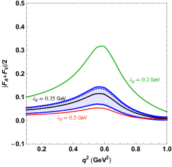
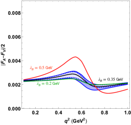
Figure 3: $\left|F_{V}+F_{A}\right|/2$ (left) and $\left|F_{A}-F_{V}\right|/2$ (right) as a function of $q^{2}$ for $p^{2}=10$ GeV². The black curve corresponds to central values of the input parameters, the dotted blue curves show the variation due to the hard-collinear scale, $\mu$ varied between $[1-2]$ GeV, the solid blue curves show the variation due to the input parameters: $m_{b},s_{0},M^{2}$, and $f_{B}$, where the errors have been added in quadrature. The green and red curves correspond to $\lambda_{B}$ = 0.2 and 0.5 GeV respectively.

3.3 Results

We will now present our predictions for the branching ratios for $B\to\ell\ell\ell^{\prime}\nu$ in the $q^{2}$ bins: $[4m_{\mu}^{2},1\,\mbox{GeV}^{2}]$ and $[0.1,1]$ GeV² as well as $[0.0025,1]$ GeV² when $\ell=e$. These results can be found in Table 2, where the final states considered are $\mu\mu\mu\nu$ and $ee\mu\nu$. It is evident that the effect of interference for the case $\ell=\ell^{\prime}$ enhances the branching ratio by $\sim$ 15$\%$. The remaining two possible final states will be discussed later on in this section. In order to understand the origin of the uncertainties on the result, we study the different contributions to the uncertainty for one of the results (for $\lambda_{B}=350$ MeV):

$$10^{7}\mathcal{BR}(B\to ee\mu\nu)\big{|}_{[\,0.1,\,1]}=\,0.411 \,+{\footnotesize\begin{pmatrix}+0.085\\ -0.140\end{pmatrix}_{\mu}+\begin{pmatrix}+0.083\\ -0.076\end{pmatrix}_{|V_{ub}|}+\begin{pmatrix}+0.012\\ -0.008\end{pmatrix}_{m_{b}}}$$

$$+{\footnotesize\begin{pmatrix}+0.012\\ -0.013\end{pmatrix}_{M^{2}}+\begin{pmatrix}+0.005\\ -0.006\end{pmatrix}_{s_{0}}+\begin{pmatrix}+0.010\\ -0.009\end{pmatrix}_{f_{B}}}.$$ (34)

We see that the largest contribution to the uncertainty, of around $20-30\%$, is due to the hard-collinear factorization scale $\mu$. This is in contrast with the radiative $B^{+}$ decay where the dependence on the scale $\mu$ nearly vanishes at NNLO. Another major source of uncertainty is the CKM matrix element $|V_{ub}|$, contributing at the $20\%$ level. Since $|V_{ub}|$ enters as an overall factor in the branching ratio, the resulting uncertainty is independent of the phase space. The mass of the $b$-quark $m_{b}$, the decay constant of the $B$ meson $f_{B}$, and the Borel parameter $M^{2}$ each provide an uncertainty of $\sim 3\%$, while the continuum threshold $s_{0}$ results in an error of only $1-2\%$.

Mode	$q^{2}$ bin (GeV2)	BR $\times(10^{7})$
$B\to\mu\mu\mu\nu$	$[4m_{\mu}^{2},1]$	$0.602^{+0.159}_{-0.158}$
	$[0.1,1]$	$0.471^{+0.121}_{-0.118}$
$B\to ee\mu\nu$	$[0.0025,1]$	$0.759^{+0.209}_{-0.276}$
	$[4m_{\mu}^{2},1]$	$0.519^{+0.152}_{-0.197}$
	$[0.1,1]$	$0.411^{+0.121}_{-0.160}$

Table 2: Branching ratios of $B\to\mu\mu\mu\nu$ and $B\to ee\mu\nu$

Note that an interesting consequence of lepton flavour universality (LFU) in SM is the branching ratios for different lepton pairs, measured in the same kinematic range, should turn out to be,

$$\mathcal{BR}(B\to eee\nu)\big{|}_{[q^{2}_{\rm low},q^{2}_{\rm high}]} =\mathcal{BR}(B\to\mu\mu\mu\nu)\big{|}_{[q^{2}_{\rm low},q^{2}_{\rm high}]}$$

$$\mathcal{BR}(B\to\mu\mu e\nu)\big{|}_{[q^{2}_{\rm low},q^{2}_{\rm high}]} =\mathcal{BR}(B\to ee\mu\nu)\big{|}_{[q^{2}_{\rm low},q^{2}_{\rm high}]}$$ (35)

In this study, we found that the relation holds upto the accuracy of the results given in Table 2. Hence, we give predictions for two decay processes, $B\to ee\mu\nu$ and $B\to\mu\mu\mu\nu$. The branching ratios of other processes follow from Eq.(3.3).

In the above discussion of the uncertainties, we have not yet mentioned the input parameter $\lambda_{B}$. The reason is that this is the very parameter we propose to measure or constrain via measurements of the branching ratios give in Table 2. Such a measurement relies crucially on the dependence of the integrated branching ratio for $B\to\ell\ell\ell^{\prime}\nu$ in the $q^{2}$ bin $[4m_{\mu}^{2},1\,\mbox{GeV}^{2}]$ on $\lambda_{B}$, we show the case of $B\to\mu\mu e\nu$ in Fig. 4. Here one sees the branching ratio in the bin $[4m_{\mu}^{2},1\,\mbox{GeV}^{2}]$ as a function of $\lambda_{B}$, where the central value is shown in black, the total uncertainty is indicated by the solid blue lines and the uncertainty band due to the hard-collinear scale is shown by the dotted blue lines. We further show the lower bound $\lambda_{B}>238$ GeV obtained by Belle mentioned in Sec. 3 [8]. There is clearly a strong dependence of this binned branching ratio on $\lambda_{B}$, far beyond the uncertainties arising from the remaining parameters. The final question to be answered is therefore whether the experiments LHCb and Belle II could possibly measure these binned branching ratios, and if so with what accuracy.

Here we stress again that the theoretical definition of $q^{2}$, i.e. the dilepton mass squared of the leptons originating from the virtual photon, can only be determined experimentally for the case $\ell\neq\ell^{\prime}$. Therefore the measurement of the integrated branching ratio in the $q^{2}$ bin we advocate can only be performed for this case. As mentioned in Sec. 1, so far the only limit on $B\to\ell\ell\ell^{\prime}\nu$ decays available is from the LHCb experiment for the case $\ell=\ell^{\prime}=\mu$, where with 4.7 fb^-1 they obtain an upper limit on the branching ratio of $1.6\times 10^{-8}$ at 95% C.L., in the region where the lowest of the two $\mu^{+}\mu^{-}$ mass combinations is below 0.98 GeV. As our formalism is only valid for low $q^{2}$, we cannot compare our results to this prediction. The sensitivity of LHCb for the case $\ell\neq\ell^{\prime}$ has not yet been studied, but given the existing limit for $\ell=\ell^{\prime}=\mu$, and taking a conservative guess that the yield would diminish by a factor of 3-4, the prospects for this channel with the the 50 ab^-1 expected by the end of Upgrade I, let alone the 300 ab^-1 at the end of Upgrade II, look very promising. For Belle II, the measurement of $B\to\gamma\ell\nu$ would probably provide a more precise measurement of $\lambda_{B}$, given the branching ratio is $\mathcal{O}(10)$ times larger [12]. With the full Belle II dataset of 50 ab^-1 expected by 2025 from Belle II, a factor $\mathcal{O}(10)$ reduction in the statistical uncertainty should be possible, more details can be found in Ref. [12]. However, a measurement of the partial branching fraction for $B\to ee\mu\nu$ and $B\to\mu\mu e\nu$, in the low $q^{2}$ bins $[0.0025,1]$ and $[0.1,1]$ GeV² respectively, could provide additional interesting information.

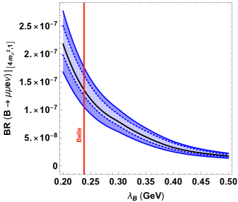
Figure 4: Integrated branching ratio of $B\to\mu\mu e\nu$ in the $q^{2}$ bin $[4m_{\mu}^{2},1\,\mbox{GeV}^{2}]$ as a function of $\lambda_{B}$. The black curve shows the central value, dotted blue curves show the variation due to the hard-collinear scale, $\mu$ varied between $[1-2]$ GeV, solid blue curves show the variation due to all input parameters, where the errors have been added in quadrature. The red line corresponds to the lower limit on $\lambda_{B}$ at 90% C.L. measured by Belle [8].

4 Conclusions

In this paper we have studied the purely leptonic decay modes $B\to\ell\ell\ell^{\prime}\nu$ for $\ell,\ell^{\prime}=e,\mu$ in the low $q^{2}$ region at NLL, including the leading $1/m_{b}$ and $q^{2}$ corrections, as well as the soft corrections at NLL. This work is motivated by the possibility to measure $\lambda_{B}$ at LHCb, since a systematic theoretical study with uncertainties for these four-lepton modes was lacking, and in light of the recent results from LHCb [13], here we have taken a first step towards achieving this goal. We stress that our result agree with those of Ref. [16] in the $q^{2}=0$ limit. We have provided a numerical comparison of the various contributions to the form factors $F_{V}$ and $F_{A}$ in Fig. 3, where we see the importance of calculating to NLL. Note that certain higher twist contributions which were calculated in the state-of-the-art $B\to\gamma\ell\nu$ analysis have been neglected here, i.e. the $1/m_{b}$ and $1/E_{\gamma}$ higher twist corrections and the twist 3 to 6 contributions to the soft correction. The effect of these missing pieces is conservatively estimated to add $\lesssim 5\%$ to the uncertainty, negligible compared to the uncertainty coming from $|V_{ub}|$. However this is only suggestive at this stage and a proper evaluation of these corrections is called for. Further, the calculation of the additional form factors which may be needed in order to account for massive leptons would be desirable.

We advocate the measurement of the partial branching fractions for $B\to ee\mu\nu$ and $B\to\mu\mu e\nu$, in the low $q^{2}$ bins $[0.0025,1]$ and $[0.1,1]$ GeV² respectively. Our results for these quantities can be found in Table 2 for $\lambda_{B}=350$ MeV and central values of the remaining parameters, where the uncertainty is at the 30% level, dominant contributions coming from $|V_{ub}|$ and the variation of the scale. We further show the dependence of the partial branching ratio on $\lambda_{B}$ in Fig. 4, and find that the dependence far outweighs the remaining uncertainties, suggesting that given a value of the partial branching ratio a measurement of $\lambda_{B}$ should be feasible. While there are no official projections for these channels at LHCb and Belle II, naive estimates show that the prospects to measure the partial branching ratio is promising. We therefore look forward to these results and to the potential measurement of $\lambda_{B}$, complementary to that of $\mathcal{B}(B\to\gamma\ell\nu)$ at Belle II.

Appendix A Hadronic matrix element

Let us define,

$$T_{\mu\rho}(p,q)=i\int d^{4}xe^{iqx}\left<0|T\{j_{\mu}^{em}(x)\bar{u}\Gamma_{\rho}b(0)\}|B(p+q)\right>.$$ (36)

The most general decomposition of the hadronic matrix element defined in Eq.  (36) is given by,

$$T_{\mu\rho}=(a~{}q^{2}+b~{}p.q)~{}g_{\mu\rho}+c~{}p_{\mu}q_{\rho}+d~{}\epsilon_{\rho\mu\lambda\sigma}p^{\lambda}q^{\sigma}.$$ (37)

The terms containing $p_{\rho}$ have been neglected since their contribution will always be proportional to the mass of lepton. Without any loss of generality, Eq. (37) can be rewritten as,

$$T_{\mu\rho}= iF_{A}~{}(g_{\mu\rho}~{}p.q-p_{\mu}q_{\rho})+\alpha~{}g_{\mu\rho}~{}p.q+\beta~{}p_{\mu}q_{\rho}+F_{e}~{}q^{2}~{}g_{\mu\rho}$$

$$+F_{V}~{}\epsilon_{\rho\mu\lambda\sigma}p^{\lambda}q^{\sigma}$$ (38)

Constraints on $T_{\mu\rho}$ can be obtained using the current conservation of em current i.e, $\partial^{\mu}j_{\mu}^{em}=0$. This is done by differentiating the correlation function in the definition of $T_{\mu\rho}$, which gives,

$$q^{\mu}T_{\mu\rho}=i(p+q)_{\rho}f_{B}$$ (39)

Using the definition in Eq. (37), this implies

$$F_{e}q^{2}=if_{B}-(\alpha+\beta)p.q$$ (40)

Using this condition,, $T_{\mu\rho}$ is reduced to,

$$T_{\mu\rho}=(iF_{A})~{}(g_{\mu\rho}~{}p.q-p_{\mu}q_{\rho})+F_{V}~{}\epsilon_{\rho\mu\lambda\sigma}~{}p^{\lambda}q^{\sigma}+if_{B}g_{\mu\rho},$$ (41)

where, $iF_{A}$ has been redefined as $iF_{A}+\beta$ for further simplification.

References

- [1] V. M. Braun, D. Yu. Ivanov, and G. P. Korchemsky. The B meson distribution amplitude in QCD. Phys. Rev., D69:034014, 2004.
- [2] M. Beneke, T. Huber, and Xin-Qiang Li. NNLO vertex corrections to non-leptonic B decays: Tree amplitudes. Nucl. Phys., B832:109–151, 2010.
- [3] Martin Beneke and Matthias Neubert. QCD factorization for and decays. Nucl. Phys., B675:333–415, 2003.
- [4] M. Beneke and T. Feldmann. Symmetry breaking corrections to heavy to light B meson form-factors at large recoil. Nucl. Phys., B592:3–34, 2001.
- [5] A. G. Grozin and M. Neubert. Asymptotics of heavy meson form-factors. Phys. Rev., D55:272–290, 1997.
- [6] S. W. Bosch, R. J. Hill, B. O. Lange, and M. Neubert. Factorization and Sudakov resummation in leptonic radiative B decay. Phys. Rev., D67:094014, 2003.
- [7] Bernard Aubert et al. A Model-independent search for the decay . Phys. Rev., D80:111105, 2009.
- [8] A. Heller et al. Search for decays with hadronic tagging using the full Belle data sample. Phys. Rev., D91(11):112009, 2015.
- [9] M. Beneke and J. Rohrwild. B meson distribution amplitude from . Eur. Phys. J. C, 71:1818, 2011.
- [10] V. M. Braun and A. Khodjamirian. Soft contribution to and the -meson distribution amplitude. Phys. Lett., B718:1014–1019, 2013.
- [11] M. Gelb et al. Search for the rare decay of with improved hadronic tagging. Phys. Rev. D, 98(11):112016, 2018.
- [12] W. Altmannshofer et al. The Belle II Physics Book. PTEP, 2019(12):123C01, 2019. [Erratum: PTEP 2020, 029201 (2020)].
- [13] Roel Aaij et al. Search for the rare decay . Submitted to: Eur. Phys. J., 2018.
- [14] A. V. Danilina and N. V. Nikitin. Four-Leptonic Decays of Charged and Neutral Mesons within the Standard Model. Phys. Atom. Nucl., 81(3):347–359, 2018. [Yad. Fiz.81,no.3,331(2018)].
- [15] A. Danilina, N. Nikitin, and K. Toms. Decays of charged -mesons into three charged leptons and a neutrino. Phys. Rev. D, 101(9):096007, 2020.
- [16] M. Beneke, V.M. Braun, Yao Ji, and Yan-Bing Wei. Radiative leptonic decay with subleading power corrections. JHEP, 07:154, 2018.
- [17] Yu-Ming Wang. Factorization and dispersion relations for radiative leptonic decay. JHEP, 09:159, 2016.
- [18] Yu-Ming Wang and Yue-Long Shen. Subleading-power corrections to the radiative leptonic decay in QCD. JHEP, 05:184, 2018.
- [19] Alexander Khodjamirian. Form-factors of and transitions and light cone sum rules. Eur. Phys. J. C, 6:477–484, 1999.
- [20] Enrico Lunghi, Dan Pirjol, and Daniel Wyler. Factorization in leptonic radiative B decays. Nucl. Phys., B649:349–364, 2003.
- [21] Christian W. Bauer, Sean Fleming, Dan Pirjol, and Iain W. Stewart. An Effective field theory for collinear and soft gluons: Heavy to light decays. Phys. Rev., D63:114020, 2001.
- [22] M. et al Tanabashi. Review of particle physics. Phys. Rev. D, 98:030001, Aug 2018.
- [23] A. Pais and S. B. Treiman. Pion Phase-Shift Information from Decays. Phys. Rev., 168:1858–1865, 1968.
- [24] R Aaij et al. Measurement of the branching fraction at low dilepton mass. JHEP, 05:159, 2013.
- [25] Roel Aaij et al. Angular analysis of the decay in the low- region. JHEP, 04:064, 2015.
- [26] S. Descotes-Genon and Christopher T. Sachrajda. Sudakov effects in form-factors. Nucl. Phys. B, 625:239–278, 2002.
- [27] S. Descotes-Genon and C.T. Sachrajda. Factorization, the light cone distribution amplitude of the B meson and the radiative decay . Nucl. Phys. B, 650:356–390, 2003.
- [28] Bjorn O. Lange and Matthias Neubert. Renormalization group evolution of the B meson light cone distribution amplitude. Phys. Rev. Lett., 91:102001, 2003.