Wiener Filter versus Recurrent Neural Network-based 2D-Channel Estimation for V2X Communications

Abstract

We compare the potential of neural network (NN)-based channel estimation with classical linear minimum mean square error (LMMSE)-based estimators, also known as Wiener filtering. For this, we propose a low-complexity recurrent neural network (RNN)-based estimator that allows channel equalization of a sequence of channel observations based on independent time- and frequency-domain long short-term memory (LSTM) cells. Motivated by Vehicle-to-Everything (V2X) applications, we simulate time- and frequency-selective channels with orthogonal frequency division multiplex (OFDM) and extend our channel models in such a way that a continuous degradation from line-of-sight (LoS) to non-line-of-sight (NLoS) conditions can be emulated. It turns out that the NN-based system cannot just compete with the LMMSE equalizer, but it also can be trained w.r.t. resilience against system parameter mismatch. We thereby showcase the conceptual simplicity of such a data-driven system design, as this not only enables more robustness against, e.g., signal-to-noise-ratio (SNR) or Doppler spread estimation mismatches, but also allows to use the same equalizer over a wider range of input parameters without the need of re-building (or re-estimating) the filter coefficients. Particular attention has been paid to ensure compatibility with the existing IEEE 802.11p piloting scheme for V2X communications. Finally, feeding the payload data symbols as additional equalizer input unleashes further performance gains. We show significant gains over the conventional LMMSE equalization for highly dynamic channel conditions if such a data-augmented equalization scheme is used.

I Introduction

Figure 1: Tapped-delay line channel model with the delay of the first channel tap set to zero.

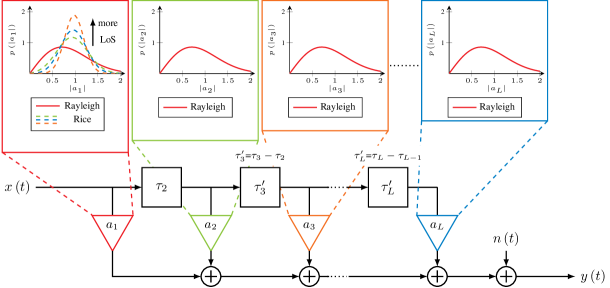
In wireless communications, high-spectral efficient data transmission strongly depends on the availability of precise knowledge of the current channel state information (CSI). Thus, the CSI needs to be estimated at the receiver – either explicitly or implicitly. In particular, for channels that are time- and frequency-selective due to motion and multi-path propagation, respectively, channel estimation becomes a key challenge in today’s OFDM-based transceiver implementations. Although channel estimation is a well-known field of classical signal processing-based research, its performance is limited by the following challenges: (a) mismatch between the mathematical traceability of the actual physical channel, i.e., an inaccuracy of the underlying channel models, (b) computational complexity and also the induced latency of the algorithms, and (c) robustness w.r.t. the system parameter estimation such as SNR or velocity. All of this leads to a discrepancy between the theoretical optimal solution and the actually achieved performance of channel equalization when deployed in a real system.

Although the channel changes continuously, the amount of transmitted pilots used for channel estimation should be as low as possible to maximize the transmission rate. Obviously, the channel state in-between pilot positions must be interpolated. Several of such pilot-aided channel estimation methods have evolved and essentially differ in the quality of this interpolation, but also in the required availability of assumptions about the channel, i.e., how is the channel correlated over time and frequency. A simple channel estimator is the least squares (LS) estimator with bilinear interpolation. The 2D-LMMSE estimator is a more advanced linear filter, which yields an optimal estimate of the channel under certain conditions [1, 2]; however, it is computationally complex and relies on the knowledge of the channel’s statistical properties, which boils down to the task of estimating the channel covariance matrix. To reduce the complexity, it can be replaced by two sequentially executed 1D-LMMSE estimators [3].

Recently, deep learning for communications has attracted a lot of attention in academia and also in industry for virtually any possible application [4, 5, 6]. This new paradigm of a data-centric system design allows to learn equalizers that are perfectly aware of the channel statistics including all its (potential) impairments. In [7] an NN structure for channel estimation is derived from the minimum mean square error (MMSE) filter. The main focus of [8] lies on the usage of additional meta data to obtain a more accurate channel estimate. Further, learning an efficient pilot arrangement together with a channel estimator for massive multiple-input multiple-output (MIMO) has been done in [9]. A joint demapping and decoding scheme is presented in [10] for a complete message frame. Further investigation on joint estimation and demapping as well as the transition towards end-to-end learning of the whole system including learning of the pilot arrangement and superimposed pilots are analyzed in [11]. It has been observed in [10] and [11] that a data-aware channel estimation can further improve the system’s performance by analyzing the payload data besides considering only the specific pilot positions. Finally, the authors of [12] propose an NN-based OFDM receiver that implicitly estimates the required CSI.

The main focus of our work is to showcase and analyze the universality and flexibility of NN-based solutions. For this, we seek to train our network over a wide range of possible input parameters. Motivated by the result in [13], which showed that RNNs are an attractive architecture for sequential data processing in communications, a novel RNN-based channel estimator is presented in this work. The presented channel estimation scheme is evaluated over time- and frequency-selective channels and compared to conventional channel estimation techniques such as 2D-LMMSE and 2x1D-LMMSE. For this, we use the piloting scheme as given in the IEEE 802.11p standard [14]. By investigating the influence of channel parameters such as velocity, noise and strength of a possible LoS connection on the accuracy of the estimated channel, we study whether it is beneficial to use an RNN-based channel estimator instead of conventional channel estimation schemes. Besides this, we analyze to what extent gains are possible while relying on inaccurate knowledge of the statistical properties and parameters of the channel. In the last section, we show that a data-augmented version of the same RNN equalizer can further extract statistical information about the channel state by observing the received payload data symbols.

II System setup

II-A Channel model

We assume a time- and frequency-selective wireless channel described by its time-variant channel impulse response

$$h\left(t,\tau\right)=\sum_{\ell=1}^{L}a_{\ell}\left(t\right)\delta\left(\tau-\tau_{\ell}\right)$$ (1)

where $L$ describes the number of channel taps, $a_{\ell}\left(t\right)$ denotes the complex-valued gain with an average power $p_{\ell}$ and $\tau_{\ell}$ represents the delay of the $\ell$-th channel tap. Each channel tap corresponds to one resolvable subpath of all paths in the multi-path environment, which is common for V2X communications. If transmitter and receiver are physically separated and there is no line-of-sight between them, the channel gain $a_{\ell}\left(t\right)$ is complex Gaussian distributed with zero-mean resulting in Rayleigh fading channel taps. This is a well-suited assumption if all received signal components are reflected or diffracted by objects of the environment. For further details we refer the reader to [15, 16]. In case there is a strong LoS component, it is more appropriate to model the first channel tap as Rician fading. The $K$-factor $K$ of the model is defined as the ratio between the power of the LoS component and the power of all the remaining resolvable multi-path components. We follow the simulation framework as described in [17].

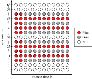
Throughout this work, we assume OFDM with cyclic prefix (CP) leading to the possibility of single-tap equalization. Let $X_{k,n}$ be the $k$-th complex symbol that should be transmitted over the $n$-th sub-carrier, where $k\in\mathbb{N}$ is the index of discrete time and $n\in\{0,...,N_{\mathrm{Sub}}-1\}$ is the sub-carrier over which the symbol should be transmitted. The symbol $X_{k,n}$ can either be a data carrying symbol or a pilot symbol that can be utilized for the channel estimation. The pilot arrangement for the IEEE 802.11p standard is schematically shown in Fig. 2. The mapping of the symbols $X_{k,n}$ onto the orthogonal sub-carriers can be expressed by an inverse discrete Fourier transform (IDFT) and to eliminate intersymbol interference (ISI) a CP is used. Let $\underline{X}_{k}=(X_{k,0},X_{k,1},...,X_{k,N_{\mathrm{Sub}}-1})^{T}$ denote the complex-valued vector containing the symbols per sub-carrier of the $k$-th OFDM symbol and $\underline{s}_{k}=(s_{k,0},s_{k,1},...,s_{k,N_{\mathrm{Sub}}-1})^{T}$ is the complex vector containing $N_{\mathrm{Sub}}$ output samples of the IDFT representing the $k$-th OFDM symbol in the time domain.

Figure 2: IEEE 802.11p pilot arrangement.

If the maximal delay of the channel is smaller than the duration of the CP, the received symbols $\underline{r}_{k}$ in the time domain after the removal of the CP are given by

$$\underline{r}_{k}=\underline{h}_{k}\circledast\underline{s}_{k}+\underline{n}_{k}$$ (2)

where $\underline{h}_{k}$ is the sampled version of the channel impulse response $h\left(t,\tau\right)$, $\underline{n}_{k}$ denotes an additive white Gaussian noise (AWGN) term and $\circledast$ denotes the circular convolution. The received symbols in the frequency domain are defined as

$$\underline{Y}_{k}{=}\underline{H}_{k}\circ\underline{X}_{k}+\underline{N}_{k}.$$ (3)

where $\underline{H}_{k}$ is the sampled channel transfer function, i.e., the discrete Fourier transform (DFT) of the sampled channel impulse response $\underline{h}_{k}$. Furthermore, $\circ$ denotes the Hadamard product, i.e., the element-wise multiplication. In the following we assume that the individual entries of $\underline{N}_{k}$ are independent and identically complex Gaussian distributed with zero-mean and a variance of $\sigma^{2}$. Hence, $\underline{N}_{k}$ is

$$\underline{N}_{k}\sim\mathcal{C}\mathcal{N}(\underline{0},\sigma^{2}\mathbf{I}_{N_{\mathrm{Sub}}})$$ (4)

distributed, where $\mathbf{I}_{N_{\mathrm{Sub}}}$ is the identity matrix of size $N_{\mathrm{Sub}}\times N_{\mathrm{Sub}}$.

At the receiver the symbols $\underline{Y}_{k}$ are equalized by scaling such that

$$\hat{Y}_{k,n}=Y_{k,n}\frac{\hat{H}_{k,n}^{*}}{|\hat{H}_{k,n}|^{2}}.$$ (5)

For the consideration of OFDM frames of $n_{\mathrm{T}}$ OFDM symbols (3) can be extended to

$$\mathbf{Y}=\mathbf{H}\circ\mathbf{X}+\mathbf{N}$$ (6)

where $\mathbf{Y}\in{\cal C}^{n_{\mathrm{T}}\times n_{\mathrm{F}}}$ is the received symbol matrix, $\mathbf{H}\in{\cal C}^{n_{\mathrm{T}}\times n_{\mathrm{F}}}$ is the channel matrix, $\mathbf{X}\in{\cal C}^{n_{\mathrm{T}}\times n_{\mathrm{F}}}$ is the transmitted symbol matrix and $\mathbf{N}\in{\cal C}^{n_{\mathrm{T}}\times n_{\mathrm{F}}}$ is the AWGN noise matrix.

((a)) 2D-Wiener filter

((b)) RNN

Figure 3: Block diagram of the 2D-Wiener filter and the RNN-based channel estimator.

Figure 4: Block diagram of the RNN-based channel estimator. The additional input $\mathbf{Y}$ is only used in Sec. IV for data-augmented channel estimation.

II-B Wiener filter baseline

The Wiener filter as shown in Fig. 3(a), also denoted as LMMSE estimator, is a linear filter that minimizes the mean squared error (MSE) between the true channel and the estimated channel. Therefore, it utilizes received pilot symbols, an estimated SNR and knowledge of the statistical properties of the channel. Precisely, it needs to know the channel’s autocorrelation function and the noise variance. For the derivation of the 2D-Wiener filter (6) is rewritten into

$$\underline{Y} =\mathbf{X}\underline{H}+\underline{N}$$ (7)

$$=\operatorname{diag}\left(\operatorname{vec}\left(\mathbf{X}\right)\right)\operatorname{vec}\left(\mathbf{H}\right)+\operatorname{vec}\left(\mathbf{N}\right)$$ (8)

where $\mathbf{X}$ is a diagonal matrix with all transmitted symbols on the main diagonal and $\underline{Y}$, $\underline{H}$ and $\underline{N}$ are the vectorized versions of the received symbols, channel matrix and the AWGN matrix, respectively. In the same way the received pilot symbols are defined as

$$\underline{Y}_{\mathrm{p}} =\mathbf{X}_{\mathrm{p}}\underline{H}_{\mathrm{p}}+\underline{N}_{\mathrm{p}}$$ (9)

$$=\operatorname{diag}\left(\Pi\operatorname{vec}\left(\mathbf{X}\right)\right)\Pi\operatorname{vec}\left(\mathbf{H}\right)+\Pi\operatorname{vec}\left(\mathbf{N}\right)$$ (10)

where $\Pi\in{\cal N}^{p\times n_{\mathrm{T}}n_{\mathrm{F}}}$ is a pilot selection matrix and $p$ is the number of pilots distributed over the OFDM frame. The pilot selection matrix contains a single one per row to select the pilot position and all the other elements of a row are set to zero.

Following [1] and [2] the channel estimate of the 2D-Wiener filter is given by

$$\hat{\underline{H}}_{\mathrm{LMMSE}}=\mathbf{W}\mathbf{X}_{\mathrm{p}}^{-1}\underline{Y}_{\mathrm{p}}$$ (11)

with the definition of the filter matrix $\mathbf{W}$

$$\mathbf{W}=\mathbf{R}_{\underline{H}\underline{H}}\Pi^{T}\left(\Pi\left(\mathbf{R}_{\underline{H}\underline{H}}+\sigma^{2}\mathbf{I}_{n_{\mathrm{T}}n_{\mathrm{F}}}\right)\Pi^{T}\right)^{-1}.$$ (12)

Note that the multiplication of $\mathbf{X}_{\mathrm{p}}^{-1}$ with $\underline{Y}_{\mathrm{p}}$ is the LS estimate of the channel at pilot positions. $\mathbf{R}_{\underline{H}\underline{H}}$ denotes the autocorrelation matrix of the channel, which we assume to be a separable composition of the temporal and the spectral autocorrelation of the channel and can be expressed as the Kronecker product [18]

$$\mathbf{R}_{\underline{H}\underline{H}}=\mathbf{R}_{\mathrm{T}}\otimes\mathbf{R}_{\mathrm{F}}.$$ (13)

This is a valid assumption for wide-sense stationary uncorrelated scattering (WSSUS) channel models. In general, the autocorrelation of unknown channels has to be determined empirically.

The temporal autocorrelation matrix $\mathbf{R}_{\mathrm{T}}$ and the spectral autocorrelation matrix $\mathbf{R}_{\mathrm{F}}$ are both Toeplitz matrices with their elements given by the temporal autocorrelation function

$$r_{\mathrm{T}}\left(kT_{\mathrm{S}}\right)=\operatorname{J_{0}}\left(2\pi f_{\mathrm{D,max}}T_{\mathrm{S}}k\right)$$ (14)

and the spectral autocorrelation function

$$r_{\mathrm{F}}\left(m\Delta f\right)=\sum_{l=0}^{L-1}p_{l}e^{j2\pi\tau_{l}\Delta fm},$$ (15)

respectively. Hereby, $T_{\mathrm{S}}$ is the duration of an OFDM symbol with CP, $f_{\mathrm{D,max}}=\nicefrac{{v}}{{c_{0}}}f_{\mathrm{c}}$ denotes the maximal Doppler frequency of the channel, $v$ denotes the velocity, $c_{0}$ is the wave propagation speed, i.e., speed of light, $f_{\mathrm{c}}$ is the carrier-frequency, $\Delta f$ is the sub-carrier spacing and $\operatorname{J_{0}}\left(.\right)$ is the zero-th order Bessel function of the first kind.

To reduce the computational complexity of the 2D-Wiener filter it can be replaced by a 2x1D-Wiener filter, considering that the two-dimensional channel estimation problem is separated into two one-dimensional tasks that are solved subsequently. The first Wiener filter interpolates the channel over the time axis, and the second Wiener filter estimates the channel over the frequency axis. For further details we refer the reader to [3], [1] and [2].

As can be seen from (12), (14) and (15) and as illustrated in Fig. 3(a), the filter matrices of the 2D-Wiener filter and the 2x1D-Wiener filter are dependent on several parameters of the channel, including velocity, noise power and $K$-factor. This additional knowledge of the channel parameters has to be provided to the Wiener filters by external parameter estimators. Furthermore, every time such a parameter changes, a recalculation of the filter matrices is required.

III RNN-based channel estimation

III-A Neural network structure and training

The structure of the proposed RNN-based channel estimator is illustrated in Fig. 4 and mainly consists of 3 bidirectional recurrent LSTM cells, which consecutively handle the input data in frequency-, then time- and then frequency-dimension again. This allows to keep the computational complexity feasible. We use recurrent NNs to exploit temporal and frequency correlations of the input data, but instead of simple recurrent neurons, we use LSTM units to circumvent the inherent vanishing gradient problem [19].

The RNN only takes the received pilot symbols $\underline{Y}_{\mathrm{p}}$, and the actually sent (known) pilot symbols $\mathbf{X}_{\mathrm{p}}$ as inputs for the two-dimensional channel estimation task. Only in Sec. IV, we additionally provide all the received symbols $\mathbf{Y}$ (including $\underline{Y}_{\mathrm{p}}$) to the RNN for data-augmented equalization. This is indicated by the red box in Fig. 4.

There are no explicit assumptions on channel statistics and noise variance fed to the RNN, but all of this information is implicitly provided through the data-driven training approach (cf. Fig. 3(b)). This is also the reason why we additionally feed $\mathbf{Y}$ (which includes random noisy payload data symbols) to the RNN (only in Sec. IV), as this allows the NN to better learn and estimate these channel statistics by itself. The first preprocessing step of the RNN-based estimator is the calculation of the LS estimate at all pilot positions $\underline{\hat{H}}_{\mathrm{p,LS}}=\mathbf{X}_{\mathrm{p}}^{-1}\underline{Y}_{\mathrm{p}}$. Thereafter, the resulting vector is reshaped into a matrix $\mathbf{\hat{H}}_{\mathrm{p,LS}}$ of target shape ${\cal C}^{n_{\mathrm{T}}\times n_{\mathrm{F}}}$ and zeros are inserted at positions where data is transmitted. Similar to [10], all inputs of shape ${\cal C}^{n_{\mathrm{T}}\times n_{\mathrm{F}}}$, including the pilot mask and positions in time and frequency dimension, are then stacked to one large input tensor.

After a complex- to real-valued conversion, the input data is processed by a bidirectional LSTM cell in frequency direction (i.e., vertically in the resource grid in Fig. 2). This means that the data (in frequency domain) is used as the LSTM cell’s time dimension. The output of the initial LSTM cell is thus an estimation for each symbol, only dependent on input data for the specific symbol and incoming cell states from decisions on previous and subsequent sub-carrier symbols. After the initial LSTM cell, the outputs are reshaped and time and frequency dimensions are transposed, so that the second LSTM cell can now operate in actual time domain (i.e., horizontally in the resource grid in Fig. 2). This second LSTM cell thereby has no direct connection in the frequency domain as its states only traverse trough the time domain. Finally, the second cell’s output is again reshaped and transposed so that a third LSTM cell can operate on frequency domain again.

The third LSTM cell’s output is then further processed by two time-distributed dense layers, i.e., dense layers that are applied to each time-frequency step separately with the same shared weights. The purpose of the first TDDL layer, which is rectified linear unit (ReLU) activated, is to combine the bidirectional LSTM cell’s forward and backward output. The second TDDL layer consists of two linearly activated neurons which finally provide an estimation on the real and imaginary part of $H_{k,n}$. We chose this 3x1D RNN structure to minimize the NN’s complexity for a single time-frequency step as much as possible with only recurrent state information traversing in time or frequency dimension. This approach renders this architecture highly scalable for all kinds of input data dimensions. Throughout this work, we use the proposed structure with 64 LSTM units per cell and 8 neurons in the first TDDL layer.

During training of the RNN-based channel estimator, stochastic gradient descent (SGD) and back-propagation through time (BPTT) are applied. Since the channel estimation problem can be classified as a regression task, we use the MSE loss; further training parameters are summarized in Tab. I. Note that, to obtain a universal channel estimator, the variety in the training data has to be high. For this, the RNN is trained within a given interval of uniformly distributed velocities and SNR values. In contrast to that, the $K$-factors used during training are not uniformly distributed, but instead, training data is divided into two halves. One half of each training batch is created with NLoS conditions, i.e., $K=0$ and the other half is created with uniformly distributed $K$-factors with $K\in(0,5)$.

TABLE I: Training parameters

Parameter	value
Epochs	100
Iterations per epoch	1000
Batch size	200
Learning rate	0.001
Velocities	0$\mathrm{\frac{km}{h}}$ - 300$\mathrm{\frac{km}{h}}$
SNR	5dB - 30dB
$K$-factors	0 - 5
Fract. of pure NLoS scenarios in train. set	50%

TABLE II: Simulation parameters

Parameter	value
Carrier frequency $f_{\mathrm{c}}$	5.9 GHz
Signal bandwidth $B$	10 MHz
OFDM symbol duration with CP $T_{\mathrm{S}}$	8 $\mathrm{\mu s}$
Cyclic prefix duration $T_{\mathrm{CP}}$	1.6 $\mathrm{\mu s}$
Sub-carrier spacing $\Delta f$	156.25 $\mathrm{kHz}$
Number of sub-carriers $N_{\mathrm{Sub}}$	64
Number of used sub-carriers	52
Pilot arrangement	IEEE 802.11p
Modulation	QPSK or 16-QAM
Channel length $L$	6 taps
Maximum delay $\tau_{\mathrm{max}}$	500 ns
PDP	equally weighted
Fading statistics	Rayleigh or Rician

III-B Simulation results

Figure 5: MSE comparison for different velocities at an SNR of 15 dB and a $K$-factor of $K=0$. The influence of up to $\pm 30$% velocity estimation mismatch on the 2D-LMMSE is visualized by the shaded red area around the LMMSE channel-matched curve.

We consider the V2X wireless channel with a carrier frequency of 5.9 GHz. The parameters assumed for the simulations are guided by the IEEE 802.11p standard [14] and are shown in detail in Tab. II. Thereby, a pilot arrangement as depicted in Fig. 2 is used.

In Fig. 5 to Fig. 8 the novel RNN-based channel estimator is compared with the 2D-Wiener filter and the 2x1D-Wiener filter (with reduced computational complexity) for varying velocities, SNR values and $K$-factors. The Wiener filters are recalculated for every evaluation point whereas the RNN-based channel estimator does not change for varying channel parameters. Besides the Wiener filters based on the accurate knowledge of the statistical properties and parameters of the channel (channel-matched LMMSE), more practicable estimated versions of them are also included (channel-mediated LMMSE) that are valid over a wider range of input parameters. Their filter matrices are estimated over $10^{6}$ channel realizations for uniformly distributed velocities between $0\mathrm{\nicefrac{{km}}{{h}}}$ and $300\mathrm{\nicefrac{{km}}{{h}}}$, SNR values between $5\mathrm{dB}$ and $30\mathrm{dB}$ and $K$-factors between $K=0$ and $K=5$. They are assumed to be applicable for a range of channel parameters and, therefore, a recalculation of the Wiener filters at runtime is not needed anymore. To summarize, the following filters are shown:

• Channel-matched LMMSE with genie-aided (perfect) parameter knowledge at the receiver. We show the 2D-LMMSE version and its 2x1D simplification for scenarios where it provides further insights.

• Channel-mediated LMMSE with estimated (averaged over many channel realizations) parameters, in an attempt to obtain an universal LMMSE estimator applicable over a wide range of parameters, serving as a best possible conventional competitor to the (later) universal RNN approach.

• RNN universal trained over a wide range of input parameters that does not require any other explicit parameter knowledge during inference.

The results reveal that the RNN-based channel estimator is universally applicable over a wide range of parameters and can adapt to varying and also difficult channel conditions, e.g., high user velocities as shown in Fig. 5. It can be seen that a high velocity renders the channel estimation into a difficult task and, thus, a general degradation of all estimators can be observed due to the high time-selectivity of the channel. Somewhat to our surprise, the RNN-based channel estimator can compete with the channel-matched LMMSE equalizer without being fed with a velocity estimation. This can be intuitively explained by the practice of training over a wide range of different channel parameters and thereby forcing the RNN to inherently learn to handle these effects solely based on input received channel observations. Note that the visible degradation of the 2x1D LMMSE performance is mainly caused by this standard’s pilot positioning scheme.

Figure 6: MSE comparison for different SNRs. The influence of up to $\pm 3$dB SNR estimation mismatch on the 2D-LMMSE is visualized by the shaded red area around the LMMSE channel-matched curve.

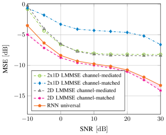
Fig. 6 analyzes the impact of the channel SNR and the red region around the LMMSE equalizer shows the influence of an $\pm 3\mathrm{dB}$ SNR parameter estimation mismatch. We want to emphasize, that the RNN-based channel estimator has an inherent advantage compared to the Wiener filter, as it only takes received channel observations as input and no further parameter estimation is required. A recalculation during runtime, as well as a separate parameter estimation block, is not needed. Therefore, this reduces its design complexity compared to a 2D-Wiener filter (assuming a continuous adaption of the filter coefficients to newly estimated parameters). Its universality and the absence of a separate parameter estimation lead to the conjecture, that the RNN implicitly learns to estimate these parameters. This is also supported by the observation that it outperforms both channel-mediated methods, which also only use the received pilot symbols without additional knowledge of the exact parameters. In cases where the 2D-Wiener filter is known to be optimal, the RNN can compete with it and is, in the most relevant regions, on par with the 2D-Wiener filter in terms of MSE performance.

Figure 7: MSE comparison for different $K$-factors at a velocity of $150\mathrm{\nicefrac{{km}}{{h}}}$ and an SNR of 15 dB.

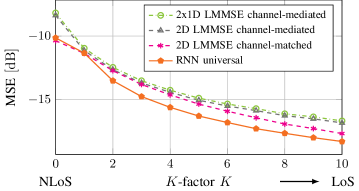
In Fig. 7 we now vary the channel properties by increasing the $K$-factor of our model. It is instructive to realize that this implies that the LoS components increasingly dominate the channel’s behavior. Note that this does not necessarily render the problem more difficult (often LoS conditions are much easier to handle; thus, the overall performance also improves for all the estimators with increasing $K$), but is simply unexpected by the equalizer and, thus, difficult to handle due to the model mismatch. Or in other words, we have designed the equalizer for the wrong channel conditions, which is beneficial for the RNN that only extracts the model from training data itself. We want to emphasize that this experiment operates the equalizers under mismatched conditions on purpose, i.e., we want to showcase the universality of the RNN-based system. Furthermore, in the case of evaluating the performance for varying $K$-factors and $K$-factors larger than zero, as shown in Fig. 7, the 2D-Wiener filter is not optimal anymore. Although, it is still the best conventional channel estimation method for this task, the RNN is able to outperform the 2D-Wiener filter for the given mismatch. However, the importance of this experiment is not necessarily found in the pure performance gain, but also in the simplicity of the system design.

Figure 8: MSE comparison for the mismatch of the velocity, for the mismatch of the SNR and for the mismatch of the $K$-factor (based on a velocity of $150\mathrm{\nicefrac{{km}}{{h}}}$, an SNR of 15 dB and a $K$-factor of 0).

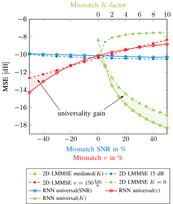
These gains in universality are also visible in Fig. 8, where the RNN’s MSE performance is compared to a mismatched LMMSE estimator, which assumes $K=0$, $v=150\mathrm{\nicefrac{{km}}{{h}}}$ and an SNR of $15\mathrm{dB}$. The shaded areas visualize regions for which the RNN provides a significantly better performance than the best LMMSE version. For readability, other estimators are not shown here. It can be clearly seen that the LMMSE equalizer performs slightly better if all parameters are well known, however, when introducing a mismatch of SNR, velocity or $K$-factor, the RNN clearly outperforms the classical approaches.

Figure 9: MSE comparison for different velocities at randomly chosen $K$-Factors between 0 and 5 (at least 20% $K=0$) and randomly chosen SNRs in the range between $5\mathrm{dB}$ and $30\mathrm{dB}$. The RNN-based equalizer now uses $\mathbf{Y}$ as additional input, i.e., data-augmented equalization is used.

Figure 10: BER vs. SNR for QAM constellations of $m=2$ and $m=4$ bit per complex symbol after soft-demapping and 40 iterations of BP decoding.

IV Data Augmented Equalization

We now extend the RNN equalizer by additionally providing the data symbols (without involving any decision feedback) to the equalizer similar to [10, 11] and, thereby, realize a data-aware equalization. This means we simply enable the additional input of $\mathbf{Y}$ in Fig. 4 (red box) and re-train the system. Note that we only re-use existing data that must be available at the receiver anyway but remains unused in the classical linear equalization schemes. The observed gains (shown in Fig. 9- 10 and discussed in the following) can intuitively be explained by the fact that the data symbols – although unknown at the receiver – can only occur at specific positions of the regular QAM constellation grid. This information is typically not used, however, the conceptual elegance of NNs easily allows to extract further statistical information about the current channel state even with data suffering from high uncertainty (unknown data bits and additional channel noise). So far the gains of the RNN-based equalizer have been limited and could be found more in terms of universality but not necessarily in terms of MSE performance gains when compared to the LMMSE equalizer. However, this experiment underlines the conceptual simplicity of such a data-driven system design w.r.t. re-using additional data sources. We simply re-train the system with the additional data input and do not need any reconsideration of the system setup itself. We empirically observe that this data augmentation provides significant additional gains in highly dynamic situations such as high velocity scenarios which would otherwise require more pilots.

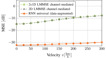
Fig. 9 shows the MSE performance at varying velocities in a scenario with $K$-factors randomly chosen between 0 to 5 with at least 20% of NLoS conditions ($K=0$) and SNR randomly chosen between $5\mathrm{dB}$ and 30$\mathrm{dB}$. Due to all channel parameters being randomly chosen, Fig. 9 only shows the channel-mediated estimators, with optimized filter coefficients for given parameter ranges, as conventional baseline. Clearly, the additional input of the received data symbols $\mathbf{Y}$ helps the RNN to track the variations of the channel and it can outperform both comparable channel-mediated 2x1D and 2D LMMSE baseline systems over the whole range of investigated velocities.

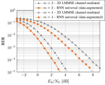
To further highlight these advantages in terms of resilience and a more accurate channel estimation, we now examine whether the observed gains for MSE on channel estimation can be transferred to the more tangible metric of final bit error rate (BER) performance. Therefore, we use $\hat{\mathbf{H}}$ to employ a posterior probability (APP) soft-demapping and add an outer irregular low-density parity-check (LDPC) code of rate $r=\nicefrac{{1}}{{2}}$, length $n=1296$ bit and 40 iterations of BP decoding. We also evaluate the BER performance in the more realistic channel scenario with parameters $K$ randomly chosen from 0 to 5 with at least 20% of NLoS ($K=0$) realizations and velocity randomly chosen between 0 and 300$\mathrm{\nicefrac{{km}}{{h}}}$ at varying SNR. Fig. 10 shows the BER performance vs. $\nicefrac{{E_{b}}}{{N_{0}}}$ for randomly generated bit, modulated with quadrature phase shift keying (QPSK) ($m=2$ bit per complex symbol) and 16-QAM ($m=4$) constellations. As can be seen, the RNN’s generally improved estimation $\mathbf{\hat{H}}_{\text{RNN}}$ in terms of MSE also leads to improved final BER performance. Thereby it is shown, that soft-values which are demapped using $\mathbf{\hat{H}}_{\text{RNN}}$ provide more information to the BP decoder at a given SNR than soft-values which are demapped using the conventional LMMSE estimator. Finally, we can observe gains in this specific scenario with varying parameters of up to 1dB for $m=2$ and even higher gains of up to 1.4dB for $m=4$. This performance increase for higher constellation orders is also expected, as higher constellations require better estimation to ensure good symbol and bit decisions.

V Conclusion and Outlook

We have shown that NN-based estimation for time- and frequency-selective channels exhibits a robust behavior w.r.t. inaccurate channel parameter knowledge. It turned out that NN-based channel estimation can compete with the (close to) optimal LMMSE estimator for a wide range of channel parameters and can even outperform the baseline for scenarios with inaccurate parameter estimations. When compared to the baseline without perfect velocity estimation and evaluated on a more realistic channel with LoS components, we observed significant gains. We have kept full compatibility to the IEEE 802.11p piloting scheme, however, extensions to other piloting schemes are straightforward. Finally, we have showcased the possibility of data-aware equalization that is able to extract further statistical information of the channel from the payload data sequence leading to significant MSE and consequently BER performance gains.

It remains open for future work to evaluate (and potentially train) the system with real-world data from larger measurement campaigns, in particular, from V2X scenarios. We want to emphasize that the main contribution of this work is not necessarily found in plain performance improvements for fixed channel setups, but to showcase the conceptual simplicity of such a data-driven and RNN-based system design.

References

- [1] R. Nilsson, O. Edfors, M. Sandell, and P. O. Borjesson, “An analysis of two-dimensional pilot-symbol assisted modulation for OFDM,” in 1997 IEEE International Conference on Personal Wireless Communications (Cat. No. 97TH8338). IEEE, 1997, pp. 71–74.
- [2] P. Hoeher, S. Kaiser, and P. Robertson, “Two-dimensional pilot-symbol-aided channel estimation by Wiener filtering,” in 1997 IEEE International Conference on Acoustics, Speech, and Signal Processing, vol. 3. IEEE, 1997, pp. 1845–1848.
- [3] X. Dong, W.-S. Lu, and A. C. Soong, “Linear interpolation in pilot symbol assisted channel estimation for OFDM,” IEEE Transactions on Wireless Communications, vol. 6, no. 5, pp. 1910–1920, 2007.
- [4] T. O’Shea and J. Hoydis, “An Introduction to Deep Learning for the Physical Layer,” IEEE Trans. Cogn. Commun. Netw., vol. 3, no. 4, pp. 563–575, Dec. 2017.
- [5] N. Farsad and A. Goldsmith, “Neural network detection of data sequences in communication systems,” IEEE Trans. on Signal Process., vol. 66, no. 21, pp. 5663–5678, 2018.
- [6] E. Nachmani, Y. Be’ery, and D. Burshtein, “Learning to decode linear codes using deep learning,” in Allerton Conf. IEEE, 2016, pp. 341–346.
- [7] D. Neumann, T. Wiese, and W. Utschick, “Learning the MMSE channel estimator,” IEEE Transactions on Signal Processing, vol. 66, no. 11, pp. 2905–2917, 2018.
- [8] C. Luo, J. Ji, Q. Wang, X. Chen, and P. Li, “Channel state information prediction for 5G wireless communications: A deep learning approach,” IEEE Transactions on Network Science and Engineering, 2018.
- [9] M. B. Mashhadi and D. Gunduz, “Pruning the pilots: Deep learning-based pilot design and channel estimation for MIMO-OFDM systems,” arXiv preprint arXiv:2006.11796, 2020.
- [10] M. Honkala, D. Korpi, and J. M. Huttunen, “Deeprx: Fully convolutional deep learning receiver,” arXiv preprint arXiv:2005.01494, 2020.
- [11] F. A. Aoudia and J. Hoydis, “End-to-end learning for OFDM: From neural receivers to pilotless communication,” arXiv preprint arXiv:2009.05261, 2020.
- [12] H. Ye, G. Ye Li, B. Juang, “Power of Deep Learning for Channel Estimation and Signal Detection in OFDM Systems,” IEEE Wireless Communications Letters, 2018.
- [13] D. Tandler, S. Dörner, S. Cammerer, and S. ten Brink, “On recurrent neural networks for sequence-based processing in communications,” in 2019 53rd Asilomar Conference on Signals, Systems, and Computers. IEEE, 2019, pp. 537–543.
- [14] I. S. Association et al., “802.11p-2010-IEEE standard for information technology-local and metropolitan area networks-specific requirements-part 11: Wireless LAN medium access control (MAC) and physical layer (PHY) specifications amendment 6: Wireless access in vehicular environments,” 2010.
- [15] A. F. Molisch, Wireless Communications, 2nd ed. John Wiley & Sons Ltd., 2016.
- [16] G. L. Stüber, Principles of Mobile Communication, 4th ed. Springer International Publishing, 2017.
- [17] C. Xiao, Y. R. Zheng, and N. C. Beaulieu, “Statistical simulation models for Rayleigh and Rician fading,” in IEEE International Conference on Communications, 2003. ICC ’03., vol. 5, 2003, pp. 3524–3529 vol.5.
- [18] M. Šimko, C. Mehlführer, M. Wrulich, and M. Rupp, “Doubly dispersive channel estimation with scalable complexity,” in 2010 International ITG Workshop on Smart Antennas (WSA), 2010, pp. 251–256.
- [19] S. Hochreiter and J. Schmidhuber, “Long short-term memory,” Neural computation, vol. 9, pp. 1735–80, 12 1997.
- [20] S. Cammerer, F. A. Aoudia, S. Dörner, M. Stark, J. Hoydis, and S. ten Brink, “Trainable communication systems: Concepts and prototype,” IEEE Transactions on Communications, vol. 68, no. 9, pp. 5489–5503, 2020.