Active Slices for Sliced Stein Discrepancy

Abstract

Sliced Stein discrepancy (SSD) and its kernelized variants have demonstrated promising successes in goodness-of-fit tests and model learning in high dimensions. Despite their theoretical elegance, their empirical performance depends crucially on the search of optimal slicing directions to discriminate between two distributions. Unfortunately, previous gradient-based optimisation approaches for this task return sub-optimal results: they are computationally expensive, sensitive to initialization, and they lack theoretical guarantees for convergence. We address these issues in two steps. First, we provide theoretical results stating that the requirement of using optimal slicing directions in the kernelized version of SSD can be relaxed, validating the resulting discrepancy with finite random slicing directions. Second, given that good slicing directions are crucial for practical performance, we propose a fast algorithm for finding such slicing directions based on ideas of active sub-space construction and spectral decomposition. Experiments on goodness-of-fit tests and model learning show that our approach achieves both improved performance and faster convergence. Especially, we demonstrate a 14-80x speed-up in goodness-of-fit tests when comparing with gradient-based alternatives.

1 Introduction

Discrepancy measures between two distributions are critical tools in modern statistical machine learning. Among them, Stein discrepancy (SD) and its kernelized version, kernelized Stein discrepancy (KSD), have been extensively used for goodness-of-fit (GOF) testing (Liu et al., 2016; Chwialkowski et al., 2016; Huggins & Mackey, 2018; Jitkrittum et al., 2017; Gorham & Mackey, 2017) and model learning (Liu & Wang, 2016; Pu et al., 2017; Hu et al., 2018; Grathwohl et al., 2020). Despite their recent success, applications of Stein discrepancies to high-dimensional distribution testing and learning remains an unsolved challenge.

These “curse of dimensionality” issues have been recently addressed by the newly proposed Sliced Stein discrepancy (SSD) and its kernelized variants SKSD (Gong et al., 2021), which have demonstrated promising results in both high dimensional GOF tests and model learning. They work by first projecting the score function and the test inputs across two slice directions $\bm{r}$ and $\bm{g}_{r}$ and then comparing the two distributions using the resulting one dimensional slices. The performance of SSD and SKSD crucially depends on choosing slicing directions that are highly discriminative. Indeed, Gong et al. (2021) showed that such discrepancy can still be valid despite the information loss caused by the projections, if optimal slices – directions along which the two distributions differ the most – are used. Unfortunately, gradient-based optimization for searching such optimal slices often suffers from slow convergence and sub-optimal solutions. In practice, many gradient updates may be required to obtain a reasonable set of slice directions (Gong et al., 2021).

We aim to tackle the above practical challenges by proposing an efficient algorithm to find good slice directions with statistical guarantees. Our contributions are as follows:

• We propose a computationally efficient variant of SKSD using a finite number of random slices. This relaxes the restrictive constraint of having to use optimal slices, with the consequence that convergence during optimisation to a global optimum is no longer required.

• Given that good slices are still preferred in practice, we propose surrogate optimization tasks to find such directions. These are called active slices and have analytic solutions that can be computed very efficiently.

• Experiments on GOF test benchmarks (including testing on restricted Boltzmann machines) show that our algorithm outperforms alternative gradient-based approaches while achieving at least a 14x speed-up.

• In the task of learning high dimensional independent component analysis (ICA) models (Comon, 1994), our algorithm converges much faster and to significantly better solutions than other baselines.

Road map:

First, we give a brief background for SD, SKSD and its relevant variants (Section 2). Next, we show that the optimality of slices are not necessary. Instead, finite random slices are enough to ensure the validity of SKSD (3.1). Despite that relaxing the optimality constraint gives us huge freedom to select slice directions, choosing an appropriate objective for finding slices is still crucial. Unfortunately, analysing SKSD in RKHS is challenging. We thus propose to analyse SSD as a surrogate objective by showing SKSD can be well approximated by SSD (Section 3.2). Lastly, by analyzing SSD, we propose algorithms to find active slices for SKSD (Sections 4, 5, 6), and demonstrate the efficacy of our proposal in the experiments (Section 7). Assumptions and proofs of theoretical results as well as the experimental settings can be found in the appendix.

2 Background

For a distributions $p$ on $\mathcal{X}\subset\mathbb{R}^{D}$ with differentiable density, we define its score function as $\boldsymbol{s}_{p}(\boldsymbol{x})=\nabla_{\boldsymbol{x}}\log p(\boldsymbol{x})$. We also define the Stein operator $\mathcal{A}_{p}$ for distribution $p$ as

$$\mathcal{A}_{p}\bm{f}(\boldsymbol{x})=\boldsymbol{s}_{p}(\boldsymbol{x})^{T}\bm{f}(\boldsymbol{x})+\nabla_{\boldsymbol{x}}^{T}\bm{f}(\boldsymbol{x})\,,$$ (1)

where $\bm{f}:\mathcal{X}\rightarrow\mathbb{R}^{D}$ is a test function. Then the Stein discrepancy (SD) (Gorham & Mackey, 2015) between two distributions $p,q$ with differentiable densities on $\mathcal{X}$ is

$$\begin{split}D_{SD}(q,p)&=\sup_{\bm{f}\in\mathcal{F}_{q}}\mathbb{E}_{q}[\mathcal{A}_{p}\bm{f}(\boldsymbol{x})]\,,\end{split}$$ (2)

where $\mathcal{F}_{q}$ is the Stein’s class of $q$ that contains test functions satisfying $\mathbb{E}_{q}[\mathcal{A}_{q}\bm{f}(\boldsymbol{x})]=0$ (also see Definition 22 in appendix B). The supremum can be obtained by choosing $\bm{f^{*}}\propto\boldsymbol{s}_{p}(\boldsymbol{x})-\boldsymbol{s}_{q}(\boldsymbol{x})$ if $\mathcal{F}_{q}$ is rich (Hu et al., 2018).

Chwialkowski et al. (2016); Liu et al. (2016) further restricts the test function space $\mathcal{F}_{q}$ to be a unit ball in an RKHS induced by a $c_{0}-$universal kernel $k:\mathcal{X}\times\mathcal{X}\rightarrow\mathbb{R}$. This results in the kernelized Stein discrepancy (KSD), which can be computed analytically:

$$\begin{split}D^{2}(q,p)&=\left(\sup_{\bm{f}\in\mathcal{H}_{k},||f||_{\mathcal{H}_{k}}\leq 1}\mathbb{E}_{q}[\mathcal{A}_{p}\bm{f}(\boldsymbol{x})]\right)^{2}\\ &=||\mathbb{E}_{q}[\bm{s}_{p}(\bm{x})k(\bm{x},\cdot)+\nabla_{\bm{x}}k(\bm{x},\cdot)]||^{2}_{\mathcal{H}_{k}}\,,\end{split}$$ (3)

where $\mathcal{H}_{k}$ is the $k$ induced RKHS with norm $||\cdot||_{\mathcal{H}_{k}}$.

2.1 Sliced kernelized Stein discrepancy

Despite the theoretical elegance of KSD, it often suffers from the curse-of-dimensionality in practice. To address this issue, Gong et al. (2021) proposed a divergence family called sliced Stein discrepancy (SSD) and its kernelized variants, under mild assumptions on the regularity of probability densities (Assumptions 1-4 in appendix B) and the richness of the kernel (Assumption 5 in appendix B). The key idea is to compare the distributions on their one dimensional slices by projecting the score $\bm{s}_{p}$ and test input $\bm{x}$ with two directions $\bm{r}$ and its corresponding $\bm{g}_{r}$, respectively. Readers are referred to appendix C for details. Despite that one cannot access all the information possessed by $\bm{s}_{p}$ and $\bm{x}$ due to the projections, the validity of the discrepancy can be ensured by using an orthogonal basis for $\bm{r}$ along with the corresponding most discriminative $\bm{g}_{r}$ directions. The resulting valid discrepancy is called maxSSD-g, which uses a set of orthogonal basis $\bm{r}\in O_{r}$ and their corresponding optimal $\bm{g}_{r}$ directions:

$$\begin{split}S_{\text{max}_{g_{r}}}(q,p)&=\sum_{\bm{r}\in O_{r}}{\sup_{\begin{subarray}{c}h_{rg_{r}}\in\mathcal{F}_{q}\\ \bm{g}_{r}\in\mathbb{S}^{D-1}\end{subarray}}{\mathbb{E}_{q}[{s}^{r}_{p}(\bm{x})h_{rg_{r}}(\bm{x}^{T}\bm{g}_{r})+}}\\ &{{\bm{r}^{T}\bm{g}_{r}\nabla_{\bm{x}^{T}\bm{g}_{r}}h_{rg_{r}}(\bm{x}^{T}\bm{g}_{r})]}}\,,\end{split}$$ (4)

where $h_{rg_{r}}:\mathcal{K}\subseteq\mathbb{R}\rightarrow\mathbb{R}$ is the test function, $\mathbb{S}^{D-1}$ is the $D$-dimensional unit sphere and $s_{p}^{r}(\bm{x})=\bm{s}_{p}(\bm{x})^{T}\bm{r}$ is the projected score function. Under certain scenarios (Gong et al., 2021), i.e. GOF test, one can further improve the performance of maxSSD-g by replacing $\sum_{\bm{r}\in O_{r}}$ with the optimal $\sup_{\bm{r}\in\mathbb{S}^{D-1}}$ in Eq.4, resulting in another variant called maxSSD-rg ($S_{\text{max}_{rg_{r}}}$). This increment in performance is due to the higher discriminative power provided by the optimal $\bm{r}$.

However, the optimal test functions $h^{*}_{rg_{r}}$ in maxSSD-g (or -rg) are intractable in practice. Gong et al. (2021) further proposed kernelized variants to address this issue by letting $\mathcal{F}_{q}$ to be in a unit ball of an RKHS induced by a $c_{0}-$universal kernel $k_{rg_{r}}$. With

$$\begin{split}\xi_{p,r,g_{r}}(\bm{x},\cdot)&=s_{p}^{r}(\bm{x})k_{rg_{r}}(\bm{x}^{T}\bm{g}_{r},\cdot)+\\ &\quad\bm{r}^{T}\bm{g}_{r}\nabla_{\bm{x}^{T}\bm{g}_{r}}k_{rg_{r}}(\bm{x}^{T}\bm{g}_{r},\cdot)\,,\end{split}$$ (5)

the maxSKSD-g (the kernelized version of maxSSD-g) is

$$SK_{\text{max}_{g_{r}}}(q,p)=\sum_{\bm{r}\in O_{r}}{\sup_{\bm{g}_{r}\in\mathbb{S}^{D-1}}{||\mathbb{E}_{q}[\xi_{p,r,g_{r}}(\bm{x})]||^{2}_{\mathcal{H}_{rg_{r}}}}}\,,$$ (6)

where $\mathcal{H}_{rg_{r}}$ is the RKHS induced by $k_{rg_{r}}$ with the associated norm $||\cdot||_{\mathcal{H}_{rg_{r}}}$. Similarly, a kernelized version of maxSSD-rg, denoted by maxSKSD-rg ($SK_{\text{max}_{rg_{r}}}$), is obtained by replacing $\sum_{\bm{r}\in O_{r}}$ with $\sup_{\bm{r}\in\mathbb{S}^{D-1}}$ in Eq.6.

Despite that maxSKSD-g (or -rg) addresses the tractability of test functions, the practical challenge of computing them is the computation of the optimal slice directions $\bm{r}$ and $\bm{g}_{r}$. Gradient-based optimization (Gong et al., 2021) for such computation suffers from slow convergence; even worse, it is sensitive to initialization and returns sub-optimal solutions only. In such case, it is unclear whether the resulting discrepancy is still valid, making the correctness of GOF test unverified. Therefore, the first important question to ask is: are the optimality of slices a necessary condition for the validity of maxSKSD-g (or -rg)? Remarkably, we show that the answer is No with mild assumptions on the kernel (Assumption 5-6 in appendix B).

As the sliced Stein discrepancy defined previously involves a $\sup$ operator, making them difficult to analyze, we need to define notations for their “sub-optimal” versions. For example, maxSSD-g (Eq.4) involves a $\sup$ operator over slices $\bm{g}_{r}$. We thus define SSD-g ($S_{g_{r}}$) as Eq.4 with a given $\bm{g}_{r}$ instead of the $\sup$:

$$\begin{split}S_{g_{r}}&=\sum_{\bm{r}\in O_{r}}\sup_{h_{rg_{r}}\in\mathcal{F}_{q}}\mathbb{E}_{q}[s_{p}^{r}(\bm{x})h_{rg_{r}}(\bm{x}^{T}\bm{g}_{r})+\\ &\bm{r}^{T}\bm{g}_{r}\nabla_{\bm{x}^{T}\bm{g}_{r}}h_{rg_{r}}(\bm{x}^{T}\bm{g}_{r})]\end{split}$$ (7)

Following similar logic, we define the “sub-optimal” version for each of the discrepancy mentioned in this section as table 1 and appendix A.

Table 1: Notations for “sub-optimal” versions of SSD & SKSD.

Optimal form	maxSSD-g ($S_{\text{max}_{g_{r}}}$)	maxSSD-rg ($S_{\text{max}_{rg_{r}}}$)	maxSKSD-g ($SK_{\text{max}_{g_{r}}}$)	maxSKSD-rg ($SK_{\text{max}_{rg_{r}}}$)
Modifications	Change $\sup_{\bm{g}_{r}}$	Change $\sup_{\bm{r},\bm{g_{r}}}$ to given	Same as maxSSD-g.	Same as maxSSD-rg
	to given $\bm{g}_{r}$ in Eq.4	$\bm{r}$, $\bm{g}_{r}$ in Eq.37 (App. C)	in Eq.6	in Eq.41 (App. C)
“sub-optimum”	SSD-g ($S_{g_{r}}$)	SSD-rg ($S_{rg_{r}}$)	SKSD-g ($SK_{g_{r}}$)	SKSD-rg ($SK_{rg_{r}}$)

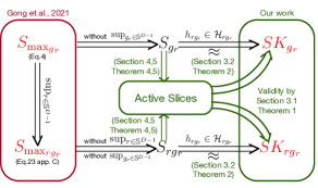
Figure 1: The relationship between different SSD discrepancies, where green texts indicate our contributions, red symbols indicate valid discrepancies and $\mathcal{H}_{rg_{r}}$ is the RKHS induced by kernel $k_{rg_{r}}$. The leftmost part are the discrepancies proposed by Gong et al. (2021), whereas the rightmost part + central “Active Slices” are our contributions. The arrows $\Rightarrow$ indicate the connections between Gong et al. (2021) and our work.

3 Relaxing constraints for the SKSD family

3.1 Is optimality necessary for validity?

As mentioned before, the discrepancy validity of max SKSD requires the optimality of slice directions, which restricts its application in practice. In the following, we show that these restrictions can be much relaxed with mild assumptions on the kernel. All proofs can be found in Appendix E.

The key idea is to use kernels such that the corresponding term $SK_{rg_{r}}$ is real analytic w.r.t. both $\bm{r}$ and $\bm{g}_{r}$, which is detailed by Assumption 6 (Appendix B). A nice property of any real analytic function is that, unless it is a constant function, otherwise the set of its roots has zero Lebesgue measure. This means the possible valid slices are almost everywhere in $\mathbb{R}^{D}$, giving us huge freedom to choose slices without worrying about violating validity.

Theorem 1 (Conditions for valid slices).

Assuming assumptions 1-4 (density regularity), 5 (richness of kernel) and 6 (real analytic kernel) in Appendix B, let $\bm{g}_{r}\sim\eta_{g}$ for each $\bm{r}\sim\eta_{r}$, where $\eta_{g}$, $\eta_{r}$ are distributions on $\mathbb{R}^{D}$ with a density, then $SK_{{rg_{r}}}(q,p)=0$ iff. $p=q$ almost surely.

The above theorem tells us that a finite number of random slices is enough to make $SK_{rg_{r}}$ valid without the need of using optimal slices (c.f. $SK_{\text{max}_{rg_{r}}}$). In practice, we often consider $\bm{r},\bm{g}_{r}\in\mathbb{S}^{D-1}$ instead of $\mathbb{R}^{D}$. Fortunately, one can easily transform arbitrary slices to $\mathbb{S}^{D-1}$ without violating the validity. For any $\bm{r},\bm{g}_{r}$, we (i) add Gaussian noises to them, and (2) re-normalize the noisy $\bm{r},\bm{g}_{r}$ to unit vectors. We refer to corollary 6.1 in appendix E.1 for details.

3.2 Relationship between SSD and SKSD

Theorem 1 allows us to use random slices. However, it is still beneficial to find good ones in practice. Unfortunately, $SK_{rg_{r}}$ is not a suitable objective for finding good slice directions. This is because, unlike the test function in a general function space ($h_{rg_{r}}\in\mathcal{F}_{q}$), the optimal kernel test function ($\mathbb{E}_{q}[\xi_{p,r,g_{r}}(\bm{x},\cdot)]$) can not be easily analyzed for finding good slices due to its restriction in RKHS.

Instead, we propose to use $S_{g}$ (or $S_{rg_{r}}$) as the optimization objective. To justify $S_{rg_{r}}$ as a good replacement for $SK_{g_{r}}$, we show that $SK_{rg_{r}}$ approximates $S_{rg_{r}}$ arbitrarily well if the corresponding RKHS of the chosen kernel is dense in continuous function space. Similar results for $SK_{g}\approx S_{g}$ can be derived accordingly as the only difference between $S_{g_{r}}$ and $S_{rg_{r}}$ is the summation over orthogonal basis $O_{r}$. However, $S_{rg_{r}}$ still involves a $\sup$ operator over test functions $h_{rg_{r}}$, which hinders further analysis. To deal with this, we give an important proposition that are needed in almost every theoretical claims we made. This proposition characterises the optimal test functions for $S_{rg_{r}}$ (or $S_{g_{r}}$).

Proposition 1 (Optimal test function given $\bm{r},\bm{g}_{r}$).

Assume assumptions 1-4 (density regularity) and given directions $\bm{r},\bm{g}_{r}$. Assume an arbitrary orthogonal matrix $\bm{G}_{r}=$ $\left[\bm{a}_{1},\ldots,\bm{a}_{D}\right]^{T}$ where $\bm{a}_{i}\in\mathbb{S}^{D\times 1}$ and $\bm{a}_{d}=\bm{g}_{r}.$ Denote $\bm{x}\sim q$ and $\bm{y}=\bm{G}_{r}\bm{x}$ which is also a random variable with the induced distribution $q_{G_{r}}$. Then, the optimal test function for $S_{rg_{r}}$ is

$$h_{rg_{r}}^{*}\left(\bm{x}^{T}\bm{g}_{r}\right)\propto\mathbb{E}_{q_{G_{r}}\left(\bm{y}_{-d}\mid y_{d}\right)}\left[\left(s_{p}^{r}\left(\bm{G}_{r}^{-1}\bm{y}\right)-s_{q}^{r}\left(\bm{G}_{r}^{-1}\bm{y}\right)\right)\right]$$ (8)

where $y_{d}=\bm{x}^{T}\bm{g}_{r}$ and $\bm{y}_{-d}$ contains other $\bm{y}$ elements.

Intuitively, assume $\bm{G}_{r}$ is a rotation matrix. Then $h_{rg_{r}}^{*}$ is the conditional expected score difference between two rotated $p$ and $q$. This form is very similar to the optimal test function for SD, which is just the score difference between the original $p$, $q$. Knowing the optimal form of $h_{rg_{r}}^{*}$, we can show $SK_{rg_{r}}$ can be well approximated by $S_{rg_{r}}$.

Theorem 2 ($SK_{rg_{r}}\approx S_{rg_{r}}$).

Assume assumptions 1-4 (density regularity) and 5 (richness of kernel). Given $\bm{r}$ and $\bm{g}_{r}$, $\forall\epsilon>0$ there exists a constant $C$ such that

$$0\leq S_{{rg_{r}}}-SK_{{rg_{r}}}<C\epsilon\,.$$

As $S_{rg_{r}}$ approximates $SK_{rg_{r}}$ arbitrary well, the hope is that good slices for $S_{rg_{r}}$ also correspond to good slices for $SK_{rg_{r}}$ in practice. Therefore in the next section we focus on analyzing $S_{rg_{r}}$ instead to propose an efficient algorithm for finding good slices.

4 Active slice direction $\bm{g}$

Finding good slices involves alternating maximization of $\bm{r}$ and $\bm{g}_{r}$. To simplify the analysis, we focus on good directions $\bm{g}_{r}$ given fixed $\bm{r}$, e.g. the orthogonal basis $\bm{r}\in O_{r}$ for now. Finding good $\bm{g}_{r}$ is achieved in two steps: (i) Rewriting the problem of the maximizing $S_{g_{r}}$ w.r.t $\bm{g}_{r}$ into an equivalent minimization problem, called controlled approximation; (ii) Establish an upper-bound of the controlled approximation objective such that its minimizer is analytic. This derivation is based on an important inequality: Poincaré inequality, which upper bounds the variances of a function by its gradient magnitude. Therefore, we need Assumptions 7-8 (Appendix B) to make sure this inequality is valid. We name the resulting $\bm{g}_{r}$ that minimizes the upper bound as active slices. All proofs can be found in appendix F.

4.1 Controlled Approximation

To start with, we need an upper bound for $S_{g_{r}}$ so that we can transform the maximization of $S_{g_{r}}$ into the minimization of their gap. Hence, we propose a generalization of SD (Eq.2) called projected Stein discrepancy (PSD):

$$\text{PSD}(q,p;O_{r})=\sum_{\bm{r}\in O_{r}}\sup_{f_{r}\in\mathcal{F}_{q}}\mathbb{E}_{q}[s^{r}_{p}(\bm{x})f_{r}(\bm{x})+\bm{r}^{T}\nabla_{\bm{x}}f_{r}(\bm{x})]$$ (9)

where $f_{r}:\mathcal{X}\subseteq\mathbb{R}^{D}\rightarrow\mathbb{R}$. SD is a special case of PSD by setting $O_{r}$ as identity matrix $\bm{I}$. In proposition 4 of appendix F.1, we show that if $\mathcal{F}_{q}$ contains all bounded continuous functions, then the optimal test function in PSD is

$$f_{r}^{*}(\bm{x})\propto\left(s_{p}^{r}(\bm{x})-s_{q}^{r}(\bm{x})\right)\,.$$ (10)

It can also be shown that PSD is equivalent to the Fisher divergence, which has been extensively used in training energy based models (Song et al., 2020; Song & Ermon, 2019) and fitting kernel exponential families (Sriperumbudur et al., 2017; Sutherland et al., 2018; Wenliang et al., 2019).

We now prove that PSD upper-bounds $S_{g_{r}}$, with the gap as the expected square error between their optimal test functions $f_{r}^{*}$ and $h^{*}_{rg_{r}}$ (Proposition 1). Since PSD is constant w.r.t. $\bm{g}_{r}$, maximization of $S_{g_{r}}$ is equivalent to a minimization task, called controlled approximation.

Theorem 3 (Controlled Approximation).

Assume assumptions 1-4 (density regularity), and the coefficient for the optimal test functions to be $1$ w.l.o.g., then $\text{PSD}\geq S_{g_{r}}$ and

$$\text{PSD}-S_{g_{r}}=\sum_{\bm{r}\in O_{r}}\mathbb{E}_{q}[(f_{r}^{*}(\bm{x})-h_{rg_{r}}^{*}(\bm{x}^{T}\bm{g}_{r}))^{2}],$$ (11)

with $f_{r}^{*}$ and $h^{*}_{rg_{r}}$ are optimal test functions for PSD and $S_{g_{r}}$ defined in Eq.10 and Eq.8 respectively.

Intuitively, minimizing the above gap can be regarded as a function approximation problem, where we want to approximate a multivariate function $f_{r}^{*}:\mathbb{R}^{D}\rightarrow\mathbb{R}$ by a univariate function $h^{*}_{rg_{r}}:\mathbb{R}\rightarrow\mathbb{R}$ with optimal parameters $\bm{g}_{r}$.

4.2 Upper-bounding the error

Solving the controlled approximation task directly may be difficult in practice. Instead, we propose an upper-bound of the approximation error, such that this upper-bound’s minimizer $\bm{g}_{r}$ is analytic. The inspiration comes from the active subspace method for dimensionality reduction (Constantine et al., 2014; Zahm et al., 2020), therefore we name the corresponding minimizers as active slices.

Theorem 4 (Error upper-bound and active slices $\bm{g}_{r}$).

Assume assumptions 2, 4 (density regularity) and 7-8 (Poincaré inequality conditions), we can upper bound the inner part of the controlled approximation error (Eq.11) by

$$\begin{split}\mathbb{E}_{q}\left[\left(f_{r}^{*}(\bm{x})-h_{rg_{r}}^{*}\left(\bm{x}^{T}\bm{g}_{r}\right)\right)^{2}\right]\leq C_{\text{sup}}\operatorname{tr}\left(\bm{G}_{r\backslash d}\bm{H}_{r}\bm{G}_{r\backslash d}^{T}\right),\end{split}$$ (12)

$$\begin{split}\bm{H}_{r}=\int q(\bm{x})\nabla_{x}f_{r}^{*}(\bm{x})\nabla_{\bm{x}}f_{r}^{*}(\bm{x})^{T}d\bm{x}.\end{split}$$ (13)

Here $C_{sup}$ is the Poincaré constant defined in assumption 8 and $\bm{G}_{r\backslash d}\in\mathbb{R}^{(D-1)\times D}$ is an arbitrary orthogonal matrix $\bm{G}_{r}$ excluding the $d^{th}$ row $\bm{g}_{r}$. The orthogonal matrix has the form $\bm{G}_{r}=[\bm{a}_{1},\ldots,\bm{a}_{D}]^{T}$ where $\bm{a}_{i}\in\mathbb{S}^{D-1}$ and $\bm{a}_{d}=\bm{g}_{r}$.

The above upper-bound is minimized when the row space of $\bm{G}_{r\backslash d}$ is the span of the first $D-1$ eigenvectors of $\bm{H}_{r}$ (arranging eigenvalues in ascending order). One possible choice for active slice $\bm{g}_{r}$ is $\bm{v}_{D}$, where $(\lambda_{i},\bm{v}_{i})$ is the eigenpair of $\bm{H}_{r}$ and $\lambda_{1}\leq\lambda_{2}\leq\ldots\leq\lambda_{D}$.

Intuitively, the active slices $\bm{g}_{r}=\bm{v}_{D}$ are the directions where the test function $f_{r}^{*}$ varies the most. Indeed, we have $\bm{v}_{D}^{T}\bm{H}_{r}\bm{v}_{D}=\mathbb{E}_{q}[||\nabla_{\bm{x}}f_{r}^{*}(\bm{x})^{T}\bm{v}_{D}||^{2}]=\lambda_{D}$, where the eigenvalue $\lambda_{D}$ measures the averaged gradient variation in the direction defined by $\bm{v}_{D}$.

5 Active slice direction $\bm{r}$

The dependence of active slice $\bm{g}_{r}$ on $\bm{r}$ motivate us to consider the possible choices of $\bm{r}$. Although finite random slices $\bm{r}$ are sufficient for obtaining a valid discrepancy, in practice using sub-optimal $\bm{r}$ can result in weak discriminative power and poor active slices $\bm{g}_{r}$. We address this issue by proposing an efficient algorithm to search for good $\bm{r}$. Again all the proofs can be found in appendix G.

5.1 PSD Maximization for searching $\bm{r}$

Directly optimizing $S_{rg_{r}}$ w.r.t. $\bm{r}$ is particularly difficult due to the alternated updates of $\bm{r}$ and $\bm{g}_{r}$. To simplify the analysis, we start from the task of finding a single direction $\bm{r}$. Our key idea to sidestep such alternation is based on the intuition that $S_{rg_{r}}$ with active slices $\bm{g}_{r}$ should well approximate $\text{PSD}_{r}$ (PSD with given $\bm{r}$) from theorem 4. The independence of $\text{PSD}_{r}$ to $\bm{g}_{r}$ allows us to avoid the alternated update and the accurate approximation validates the direct usage of the resulting active slices in $S_{rg_{r}}$. Indeed, we will prove that maximizing $\text{PSD}_{r}$ is equivalent to maximizing a lower-bound for $S_{rg_{r}}$.

Assume we have two slices $\bm{r}_{1}$ and $\bm{r}_{2}$, with given $\bm{g}_{r_{1}}$, $\bm{g}_{r_{2}}$. Then finding good $\bm{r}_{1}$ is equivalent to maximizing the difference $S_{{r_{1},g_{r_{1}}}}-S_{{r_{2},g_{r_{2}}}}$. The following proposition establishes a lower-bound for this difference.

Proposition 2 (Lower-bound for the $S_{rg_{r}}$ gap).

Assume the conditions in theorem 4 are satisfied, then for any slices $\bm{r}_{1}$, $\bm{r}_{2}$ and $\bm{g}_{r_{1}}$, $\bm{g}_{r_{2}}$, we have

$$\begin{split}S_{{r_{1},g_{r_{1}}}}-S_{{r_{2},g_{r_{2}}}}\geq\text{PSD}_{r_{1}}-\text{PSD}_{r_{2}}-C_{\text{sup}}\Omega,\end{split}$$ (14)

where $C_{\text{sup}}$ is the Poincaré constant defined in assumption 8 and $\Omega=\sum_{i=1}^{D}{\omega_{i}}$ where $\{\omega_{i}\}_{i}^{D}$ is the eigenvalue of $\mathbb{E}_{q}[\nabla_{\bm{x}}\bm{f}^{*}(\bm{x})\nabla_{\bm{x}}\bm{f}^{*}(\bm{x})^{T}]$, $\bm{f}^{*}(\bm{x})=\bm{s}_{p}(\bm{x})-\bm{s}_{q}(\bm{x})$.

Proposition 2 justifies the maximization of $\text{PSD}_{r_{1}}$ w.r.t. $\bm{r}_{1}$ as a valid surrogate. But more importantly, this alternative objective admits an analytic maximizer of $\bm{r}$, which is then used as the active slice direction:

Theorem 5 (Active slice $\bm{r}$).

Assuming assumptions 1-4 (density regularity), then the maximum of the $\text{PSD}_{r}$ is achieved at $\bm{r}^{*}=\bm{v}_{\text{max}}$:

$$\max_{\bm{r}\in\mathbb{S}^{D-1}}\mathbb{E}_{q}\left[s_{p}^{r}(\bm{x})f^{*}_{r}(\bm{x})+\bm{r}^{T}\nabla_{\bm{x}}f^{*}_{r}(\bm{x})\right]=\lambda_{\text{max}}.$$

Here $\left(\lambda_{\text{max}},\bm{v}_{\text{max}}\right)$ is the largest eigenpair of the matrix $\bm{S}=\mathbb{E}_{q}\left[\bm{f}^{*}(\bm{x})\bm{f}^{*}(\bm{x})^{T}\right]$

5.2 Constructing the orthogonal basis $O_{r}$

Under certain scenarios, e.g. model learning, we want to train the model to perform well in every directions instead of a particular one. Thus, using a good orthogonal basis is preferred over a single active slice $\bm{r}$. Here gradient-based optimization is less suited as it breaks the orthogonality constraint. Also proposition 2 is less useful here as well, as PSD is invariant to the choice of $O_{r}$, i.e. $\text{PSD}(q,p;O_{r_{1}})=\text{PSD}(q,p;O_{r_{2}})$ and $O_{r_{1}}\neq O_{r_{2}}$.

Inspired by the analysis of single active $\bm{r}$, we propose to use the eigendecomposition of $\bm{S}$ to obtain a good orthogonal basis $O_{r}$. Theoretically, this operation also corresponds to a greedy algorithm, where in step $i$ it searches for the optimal direction $\bm{r}_{i}$ that is orthogonal to $\{\bm{r}_{<i}\}$ and maximizes $\text{PSD}_{\bm{r}_{i}}$ (see Corollary 6.2 in appendix G.3). Although there is no guarantee for finding the optimal $O_{r}$ due to its myopic behavior, in practice this greedy algorithm at least finds some good directions with high discriminative power (eigenvectors with large eigenvalues).

6 Practical algorithm

Algorithm 1 Active slice algorithm

  Input: Samples $\bm{x}\sim q$, density $p$, kernel $k:\mathcal{X}\times\mathcal{X}\rightarrow\mathbb{R}$, Gaussian noise $\gamma$, pruning factor $m$ (optional)

  Result: $\widetilde{O_{r}}$, $\bm{G}$

  Estimate $\bm{s}_{p}(\bm{x})-\bm{s}_{q}(\bm{x})$ using KE or GE with kernel $k$ and samples $\bm{x}$.

  if Pruning then

     Top $m$ eigenvectors of $\bm{S}$ to form $\widetilde{O_{r}}$ (Theorem 5)

  else

     Getting all eigenvectors of $\bm{S}$ to form $\widetilde{O_{r}}$

  end if

  Add noise $\gamma$ to $\widetilde{O_{r}}$, then normalize. (Section 3.1)

  for $\bm{r}\in\widetilde{O_{r}}$ do

     $\bm{g}_{r}$ is the top 1 eigenvector of $\bm{H}_{r}$ (Theorem 4)

     Add noise $\gamma$ to $\bm{g}_{r}$ then normalize (Section 3.1)

     Concatenate $\bm{g}_{r}$ to $\bm{G}$

  end for

  Further optimize $\widetilde{O_{r}}$, $\bm{G}$ with SKSD-g ($SK_{g_{r}}$) using gradient-based optimization (Optional)

  Return: $\widetilde{O_{r}}$, $\bm{G}$

The proposed active slice method is summarized in Algorithm 1, which requires the intractable score difference $\bm{s}_{p}(\bm{x})-\bm{s}_{q}(\bm{x})$. Two types of approximations can be used. The first approach applies gradient estimators (GE) to estimate $\bm{s}_{q}(\bm{x})$ from $\bm{x}$ samples. We use the Stein gradient estimator (Li & Turner, 2017) for the GE approach, although other estimators (Sriperumbudur et al., 2017; Sutherland et al., 2018; Shi et al., 2018; Zhou et al., 2020) can also be employed. The second method directly estimates the score difference using a kernel-smoothed estimator (KE):

$$\bm{s}_{p}(\bm{y})-\bm{s}_{q}(\bm{y})\approx \mathbb{E}_{\bm{x}\sim q}[(\bm{s}_{p}(\bm{x})-\bm{s}_{q}(\bm{x}))k(\bm{x},\bm{y})]$$ (15)

$$= \mathbb{E}_{\bm{x}\sim q}[\bm{s}_{p}(\bm{x})k(\bm{x},\bm{y})+\nabla_{\bm{x}}k(\bm{x},\bm{y})],$$

where the second expression comes from integration by part, and it can be computed in practice. Figure 1 summarizes the relationships between different SSD discrepancies and highlights our contributions. For GOF test specifically, we also derive the asymptotic distribution and propose an practical GOF algorithm in appendix D.

6.1 Computational cost

The overall complexity includes the cost for (1) finding active slices (algorithm 1) (2) applying the downstream test. For finding the active slices $\bm{r}$, one important fact is that we only need the $m$ ($m\ll D$) most important $\bm{r}$ (importance characterised by eigenvalues). Luckily, fast eigenvalue-decomposition algorithm, e.g. randomized SVD from Saibaba et al. (2021), requires $O(m)$ matrix-vector product. For $\bm{g}$, from algorithm 1, we only need to solve $m$ eigenvalue-decomposition, each only cares about the most important eigenvector. Therefore, $O(m\times 1)$ matrix-vector product are needed. So the overall complexity for finding slices is $O(mD^{2})$, where $D^{2}$ comes from matrix-vector product. For gradient-based optimization (GO), the complexity is $O(l(D^{2}+C_{\text{grad}}))$ ($l$ is optimization step and $C_{\text{grad}}$ is the back-prop cost, $D^{2}$ coms from evaluating $SK_{g_{r}}$ or $SK_{rg_{r}}$). Our algorithm in general has lower training cost as $l\gg m$ and $C_{\text{grad}}$ can be expensive. For (2), our method has $O(mD)$ cost compared to $O(D^{2})$ for GO. As $m\ll D$, active slices have less complexity compared to pure GO based method proposed in Gong et al. (2021). For memory cost, our method costs $O(mD)$ to store $\bm{r},\bm{g}$ whereas GO uses $O(D^{2})$. Overall, our method requires nearly an order of magnitude less complexity in terms of computation and memory consumption.

7 Experiments

GOF test aims to test the fitness of the model to the target data. The test procedure roughly proceeds as: (1) Define null hypothesis (model matches the data distribution) and alternative hypothesis (model does not match the data distribution); (2) Compute test statistic (e.g. KSD) and threshold (e.g. bootstrap method); (3) Reject null hypothesis (statistic $>$ threshold) or not (statistic $\leq$ threshold). Refer to appendix D for more details.

7.1 Benchmark GOF tests

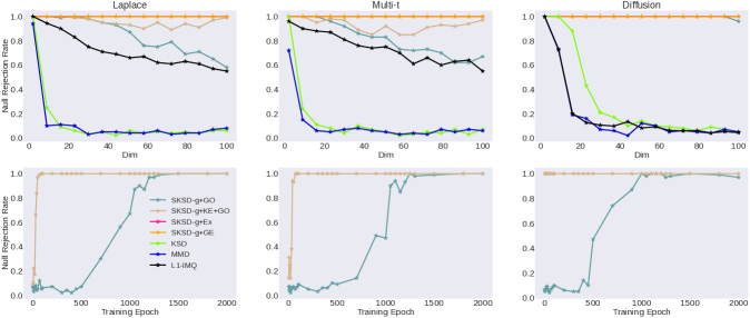
Figure 2: (Upper panel): The null rejection rate w.r.t. different dimensional benchmark problems. SKSD-g+Ex and SKSD-g+GE coincide at the optimal rejection rate (Lower panel): Null rejection rate with different number of gradient optimization epochs.

We demonstrate the improved test power results (in terms of null rejection rates) and significant speed-ups of the proposed active slice algorithm on 3 benchmark tasks, which have been extensively used for measuring GOF test performances (Jitkrittum et al., 2017; Huggins & Mackey, 2018; Chwialkowski et al., 2016; Gong et al., 2021). Here the test statistic is based on SKSD-g ($SK_{g_{r}}$) with fixed basis $O_{r}=\bm{I}$. Two practical approaches are considered for computing the active slice $\bm{g}_{r}$: (i) gradient estimation with the Stein gradient estimator (SKSD-g+GE), and (ii) gradient estimation with the kernel-smoothed estimator (KE), plus further gradient-based optimization (SKSD-g+KE+GO). For reference, we include a version of the algorithm with exact score difference (SKSD-g+Ex) as an ablation for the gradient estimation approaches.

In comparison, we include the following strong baselines: KSD with RBF kernel (Liu et al., 2016; Chwialkowski et al., 2016), maximum mean discrepancy (MMD, Gretton et al., 2012) with RBF kernel, random feature Stein discrepancy with L1 IMQ kernel (L1-IMQ, Huggins & Mackey, 2018), and the current state-of-the-art — maxSKSD-g with random initialized $\bm{g}_{r}$ followed by gradient optimization (SKSD-g+GO, Gong et al., 2021). For all methods requiring GO or active slices, we split the $1000$ test samples from $q$ into $800$ test and $200$ training data, where we run GO or active slice method on the training set.

The 3 GOF test benchmarks, with details in appendix H.1, are: (1) Laplace: $p(\bm{x})=\mathcal{N}(0,\bm{I})$, $q(\bm{x})=\prod_{d=1}^{D}{\text{Lap}(x_{d}|0,1/\sqrt{2})}$; (2) Multivariate-t: $p(\bm{x})=\mathcal{N}(0,\frac{5}{3}\bm{I})$, $q(\bm{x})$ is a fully factorized multivariate-t with $5$ degrees of freedom, $0$ mean and scale $1$; (3) Diffusion: $p(\bm{x})=\mathcal{N}(0,\bm{I})$, $q(\bm{x})=\mathcal{N}(\bm{0},\bm{\Sigma}_{1})$ where in $q(\bm{x})$ the variance of $1^{\text{st}}$-dim is $0.3$ and the rest is $\bm{I}$.

The upper panels in Figure 2 show the test power results as the dimensions $D$ increase. As expected, KSD and MMD with RBF kernel suffer from the curse-of-dimensionality. L1-IMQ performs relatively well in Laplace and multivariate-t but still fails in diffusion. For SKSD based approaches, SKSD-g+GO with $1000$ training epochs still exhibits a decreasing test power in Laplace and multivariate-t. On the other hand, SKSD-g+KE+GO with 50 training epochs has nearly optimal performance. SKSD-g+Ex and SKSD-g+GE achieve the true optimal rejection rate without any GO. Specifically, Table 2 shows that the active slice method achieves significant computational savings with 14x-80x speed-up over SKSD-g+GO.

For approaches that require gradient optimization, the lower panels in Figure 2 show the test power as the number of training epochs increases. SKSD-g+GO with random slice initialization requires a huge number of gradient updates to obtain reasonable test power, and $1000$ epochs achieves the best balance between run-time and performance. On the other hand, SKSD-g+KE+GO with active slice achieves significant speed-ups with near-optimal test power using around 50 epochs on Laplace and Multivariate-t. Remarkably, on Diffusion test, $\bm{g}_{r}$ initialized by the active slices achieves near-optimal results already, so that the later gradient refinements are not required.

Table 2: Test power for 100 dimensional benchmarks and time consumption. The run-time for SKSD-g+KE+GO include both the active slice computation and the later gradient-based refinement steps. NRR stands for null rejection rate.

	Laplace			Multi-t			Diffusion
Method	NRR	sec/trial	Speed-up	NRR	sec/trial	Speed-up	NRR	sec/trial	Speed-up
SKSD-g+Ex	1	0.38	103x	1	0.49	90x	1	0.34	102x
SKSD-g+GO	0.58	39.39	1x	0.67	44.24	1x	0.96	34.73	1x
SKSD-g+KE+GO	0.99	2.72	14x	0.97	2.38	19x	1	0.43	81x
SKSD-g+GE	1	0.66	60x	1	0.67	66x	1	0.78	44x

7.2 RBM GOF test

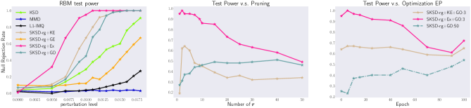
Figure 3: (Left): The GOF test power of each method with different level of noise perturbations (Mid): The effect of different pruning level towards the test power (Right): The effect of gradient based optimization epoch to the test power. 3 and 50 indicates the pruning level. KE+GO or Ex+GO means active slices with further gradient refinement steps.

Following Gong et al. (2021), we conduct a more complex GOF test using restrict Boltzman machines (RBMs, (Hinton & Salakhutdinov, 2006; Welling et al., )). Here the $p$ distribution is an RBM: $p(\bm{x})=\frac{1}{Z}\exp\left(\mathbf{x}^{\top}\mathbf{B}\mathbf{h}+\mathbf{b}^{\top}\mathbf{x}+\mathbf{c}^{\top}\mathbf{x}-\frac{1}{2}\|\mathbf{x}\|^{2}\right)$, where $\bm{x}\in\mathbb{R}^{D}$ and $\bm{h}\in\{\pm 1\}^{d_{h}}$ denotes the hidden variables. The $q$ distribution is also an RBM with the same $\mathbf{b},\mathbf{c}$ parameters as $p$ but a different $\bm{B}$ matrix perturbed by different levels of Gaussian noise. We use $D=50$ and $d_{h}=40$, and block Gibbs sampler with $2000$ burn-in steps. The test statistics for all the approaches are computed on a test set containing 1000 samples from $q$.

The test statistic is constructed using SKSD-rg ($SK_{rg_{r}}$) with $\bm{r}$, $\bm{g}_{r}$ obtained either by gradient-based optimization (SKSD-rg+GO) or the active slice algorithms (+KE, +GE and +Ex) without the gradient refinements. Specifically, SKSD-rg+GO runs 50 training epochs with $\bm{r}$ and $\bm{g}_{r}$ initialized to $\bm{I}$. For the active slice methods, we also prune away most slices and only keep the top-$3$ most important $\bm{r}$ slices.

The left panel of Figure 3 shows that SKSD-rg+KE achieves the best null rejection rates among all baselines, except for SKSD-rg+Ex whose performance is expected to upper-bound all other active slice methods. This shows the potential of our approach with an accurate score difference estimator. Although SKSD-rg+GO performs reasonably well, its run-time is 53x longer than SKSD-rg+KE as shown in Table 4. Interestingly, SKSD-rg+GE performs worse than KSD due to the significant under-estimation of the magnitude of $\bm{s}_{q}(\bm{x})$. Therefore, we omit this approach in the following ablation studies.

Ablation studies

The first ablation study, with results shown in the middle panel in Figure 3, considers pruning the active slices at different pruning levels, where the horizontal axis indicates the number of $\bm{r}$ slices used to construct the test statistic. We observe that the null rejection rates of active slice methods peak with pruning level 3, indicating their ability to select the most important directions. Their performances decrease when more $\bm{r}$ are considered since, in practice, those less important directions introduce extra noise to the test statistic. On the other hand, SKSD-rg+GO shows no pruning abilities due to its sensitivity to slice initialization. Remarkably, the final performance of SKSD-rg+GO without pruning is still worse than SKSD-rg+KE with pruning, showing the importance of finding ’good’ instead of many ’average-quality’ directions. Another advantage of pruning is to reduce the computational and memory costs from $O(MD)$ to $O(mD)$, where $m$ and $M$ are the number of pruned $\bm{r}$ and slice initializations, respectively ($m\ll M$).

The second ablation study investigates the quality of the obtained slices either by gradient-based optimization or by the active slice approaches. Results are shown in the right panel of Figure 3, where the horizontal axis indicates the number of training epochs, and the numbers annotated in the legend ($3$ and $50$) indicate the pruning. We observe that the null rejection rate of SKSD-rg+KE+GO starts to improve only after $100$ epochs, meaning that short run of GO refinements are redundant due to the good quality of active slices. The performance decrease of SKSD-rg+Ex+GO is due to the over-fitting of GO to the training set. The null rejection rate of SKSD-rg+GO gradually increases with larger training epochs as expected. However, even after 100 epochs, the test power is still lower than active slices without any GO.

In appendix H.2, another ablation study also shows the advantages of good $\bm{r}$ compared to using random slices.

7.3 Model learning: ICA

Table 3: The test NLL of different dimensional ICA model

Dimensions	SKSD-g+KE+GO	SKSD-g+Ex+GO	SKSD-g+GO	SKSD-rg+GO	LSD	KSD
10	7.93$\pm$0.31	7.95$\pm$0.31	8.06$\pm$0.33	10.03$\pm$0.61	7.42$\pm$0.31	7.82$\pm$0.31
80	7.88$\pm$0.77	15.17$\pm$0.97	19.03$\pm$1.06	62.53$\pm$0.92	6.26$\pm$1.49	80.75$\pm$1.22
100	6.93$\pm$1.36	21.50$\pm$1.41	22.22$\pm$1.08	75.28$\pm$1.63	17.55$\pm$1.60	110.78$\pm$1.19
150	11.67$\pm$2.46	27.37$\pm$3.04	21.63$\pm$3.27	107.25$\pm$1.93	32.15$\pm$3.75	180.47$\pm$1.91

We evaluate the performance of the active slice methods in model learning by training an independent component analysis (ICA) model, which has been extensively used to evaluate algorithms for training energy-based models (Gutmann & Hyvärinen, 2010; Hyvärinen & Dayan, 2005; Ceylan & Gutmann, 2018; Grathwohl et al., 2020). ICA follows a simple generative process: it first samples a $D$-dimensional random variable $\bm{z}$ from a non-Gaussian $p_{z}$ (we use multivariate-t), then transforms $\bm{z}$ to $\bm{x}=\bm{W}\bm{z}$ with a non-singular matrix $\bm{W}\in\mathbb{R}^{D\times D}$. The log-likelihood is $\log p(\bm{x})=\log p_{z}(\bm{W}^{-1}\bm{x})+C$ where $C$ can be ignored if trained by minimizing Stein discrepancies. We follow Grathwohl et al. (2020); Gong et al. (2021) to sample $20000$ training and $5000$ test datapoints from a randomly initialized ICA model. The baselines considered include KSD, SKSD-g+GO, SKSD-rg+GO and the state-of-the-art learned Stein discrepancy (LSD) (Grathwohl et al., 2020), where the test function is parametrized by a neural network. For active slice approaches, one optimization epoch include the following two steps: (i) finding active slices for both orthogonal basis $O_{r}$ and $\bm{g}_{r}$ at the beginning of the epoch, and (ii) refining the $\bm{g}_{r}$ directions and the $\bm{W}$ parameters in an adversarial manner with $O_{r}$ fixed.

Table 4: Test power and time consumption at 0.01 perturbation

	Test Power	Opt. Time	Speed-up
SKSD-rg+Ex	0.95	0.04s	254x
SKSD-rg+KE	0.67	0.19s	53x
SKSD-rg+GO	0.45	10.15s	1x

For SKSD-g+GO, we fix basis $O_{r}=\bm{I}$ and only update $\bm{g}_{r}$ with GO. We refer to appendix H.3 for details on the setup and training procedure.

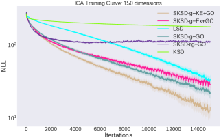
Figure 4: Training Curve of ICA model, where y-axes indicates the test NLL.

We see from Figure 4 that SKSD-g+KE+GO converges significantly faster at $150$ dimensions than all baselines; moreover, it has much better NLL (Table 3). We argue this performance gain is due to the use of the better orthogonal basis $O_{r}$ found by the greedy algorithm, showing the advantages of better $O_{r}$ in model learning. On the other hand, the importance of orthogonality in $O_{r}$ is indicated by the poor performance of SKSD-rg+GO, as gradient updates for $\bm{r}$ violate the orthogonality constraint. The goal of learning is to train the model to match the data distribution along every slicing direction, and the orthogonality constraint can help prevent the model from ignoring important slicing directions.

Interestingly, SKSD-g+Ex+GO performs worse than +KE+GO. We hypothesize that this is because the +Ex+GO approach often focuses on directions with large discriminative power but with less useful learning signal (see appendix H.3). $LSD$ performs well in low dimensional problems. However, in high dimensional learning tasks it spends too much time on finding good test functions, which slows down the convergence significantly.

8 Related Work

Active subspace method (ASM):

ASM is initially proposed as a dimensionality reduction method, which constructs a subspace with low-rank projectors (Constantine et al., 2014) according to the subspace Poincaré inequality. Zahm et al. (2020) showed promising results on the application of ASM to approximating multivariate functions with lower dimensional ones. However, they only considered the subspace Poincaré inequality under Gaussian measures, and a generalization to a broader family of famlity is proposed by Parente et al. (2020). Another closely related approach uses logarithmic Sobolev inequality instead to construct the active subspace (Zahm et al., 2018), which can be interpreted as finding the optimal subspace to minimize a KL-divergence. It has shown successes in Bayesian inverse problems and particle inference (Chen et al., 2019). However, as the ASM method is based on the eigen-decomposition of the sensitivity matrix, there is a potential limitation when the sensitivity matrix is estimated by Monte-Carlo method. We prove this limitation in appendix I.

Sliced discrepancies:

Existing examples of sliced discrepancies can be roughly divided into two groups. Most of them belong to the first group, and they use the slicing idea to improve computational efficiency. For example, sliced Wasserstein distance projects distributions onto one dimensional slices so that the corresponding distance has an analytic form (Kolouri et al., 2019; Deshpande et al., 2019). Sliced score matching uses Hutchinson’s trick to avoid the expensive computation of the Hessian matrix (Song et al., 2020). The second group focuses on the curse-of-dimensionality issue which remains to be addressed. To the best of our knowledge, existing integral probability metrics in this category include SSD (Gong et al., 2021) and kernelized complete conditional Stein discrepancy (KCC-SD, Singhal et al., 2019). The former is more general and requires less restrictive assumptions, while the latter requires samples from complete conditional distributions. Recent work has also investigated the statistical properties of sliced discrepancies (Nadjahi et al., 2020).

9 Conclusion

We have proposed the active slice method as a practical solution for searching good slices for SKSD. We first prove that the validity of the kernelized discrepancy only requires finite number of random slices instead of optimal ones, giving us huge freedom to select slice directions. Then by analyzing the approximation quality of SSD to SKSD, we proposed to find active slices by optimizing surrogate optimization tasks. Experiments on high-dimensional GOF tests and ICA training showed the active slice method performed the best across a number of competitive baselines in terms of both test performance and run-time. Future research directions include better score difference estimation methods, non-linear generalizations of slice projections, and the application of the active slice method to other discrepancies.

Appendix A Terms and Notations

For the clarity of the paper, we give a summary of the commonly used notations in the main text and proof.
Symbols:
$\bm{s}_{p}(\bm{x})$ $\nabla_{\bm{x}}\log p(\bm{x})$ $s_{p}^{r}(\bm{x})$ Projected score function $\nabla_{\bm{x}}\log p(\bm{x})^{T}\bm{r}$ $\mathcal{X}$ A subset of $\mathbb{R}^{D}$ $\mathcal{K}$ A subset of $\mathbb{R}$. $k_{rg_{r}}$ kernel function $k:\mathcal{K}\times\mathcal{K}\rightarrow\mathcal{R}$ $\mathcal{H}_{rg_{r}}$ Induced RKHS by the kernel $k_{rg_{r}}$. $||\cdot||_{\mathcal{H}_{rg_{r}}}$ RKHS norm of $\mathcal{H}_{rg_{r}}$ $\bm{g}_{r}$ Input projection direction (e.g. $\bm{x}^{T}\bm{g}_{r}$) for corresponding $\bm{r}$. $\bm{r}$ Score projection direction (e.g. $s_{p}^{r}(\bm{x})=\bm{s}_{p}(\bm{x})^{T}\bm{r}$) $S_{\text{max}_{g_{r}}}$ maxSSD-g (Eq.4). $S_{{g_{r}}}$ SSD-g, i.e. $S_{\text{max}_{g_{r}}}$ (Eq.4) without $\sup_{\bm{g}_{r}}$. But with summation of $O_{r}$. $S_{{rg_{r}}}$ SSD-rg, i.e. $S_{\text{max}_{g_{r}}}$ (Eq.4) without $\sup_{\bm{g}_{r}}$ and summation of $O_{r}$. Instead, we use specific $\bm{r}$. $SK_{\text{max}_{g_{r}}}$ maxSKSD-g. The kernelized verison of $S_{\text{max}_{g_{r}}}$ $SK_{{g_{r}}}$ SKSD-g. The kernelized verison of $S_{{g_{r}}}$ $SK_{{rg_{r}}}$ SKSD-rg. The kernelized verison of $S_{{rg_{r}}}$ PSD Projected Stein discrepancy (Eq.9) $\text{PSD}_{r}$ Projected Stein discrepancy (Eq.9) without summation $O_{r}$ and use specific $\bm{r}$ instead. $f_{r}^{*}$ Optimal test function for PSD. $f_{r}^{*}(\bm{x})\propto s_{p}^{r}(\bm{x})-s_{q}^{r}(\bm{x})$ $h_{rg_{r}}^{*}$ Optimal test function for $S_{g_{r}}$ with specific $\bm{r}$ and $\bm{g}_{r}$, defined in Eq.8. ^∗ This indicates the optimal test function (e.g. $f_{r}^{*}$) $C_{\text{sup}}$ Supremum of Poincaré constant defined in assumption 6.

A.1 “Sub-optimal” variants of SSD

For the ease of the analysis, we want to define the notations without the $\sup$ opeartor over the slice directions $\bm{r}$, $\bm{g}_{r}$. Here, we define SSD-g ($S_{g_{r}}$) as the maxSSD-g ($S_{\text{max}_{g_{r}}}$ in Eq.4) without the $\sup_{\bm{g}_{r}}$.

$$\begin{split}S_{g_{r}}&=\sum_{\bm{r}\in O_{r}}\sup_{h_{rg_{r}}\in\mathcal{F}_{q}}\mathbb{E}_{q}[s_{p}^{r}(\bm{x})h_{rg_{r}}(\bm{x}^{T}\bm{g}_{r})+\\ &\bm{r}^{T}\bm{g}_{r}\nabla_{\bm{x}^{T}\bm{g}_{r}}h_{rg_{r}}(\bm{x}^{T}\bm{g}_{r})]\end{split}$$ (16)

Similarly, we define SSD-rg ($S_{rg_{r}}$) as maxSSD-rg ($S_{\text{max}_{rg_{r}}}$ in Eq.37) without $\sup_{\bm{r},\bm{g}_{r}}$:

$$\begin{split}S_{rg_{r}}&=\sup_{h_{rg_{r}}\in\mathcal{F}_{q}}\mathbb{E}_{q}[s_{p}^{r}(\bm{x})h_{rg_{r}}(\bm{x}^{T}\bm{g}_{r})+\\ &\bm{r}^{T}\bm{g}_{r}\nabla_{\bm{x}^{T}\bm{g}_{r}}h_{rg_{r}}(\bm{x}^{T}\bm{g}_{r})]\end{split}$$ (17)

As for each of the above ”optimal” discrepancies, it has the corresponding kernelized version. Therefore, we need to define their ”un-optimal” version as well. We define SKSD-g ($SK_{g_{r}}$) as maxSKSD-g ($SK_{\text{max}_{g_{r}}}$ in Eq.6) as

$$SK_{{g_{r}}}=\sum_{\bm{r}\in O_{r}}{{||\mathbb{E}_{q}[\xi_{p,r,g_{r}}(\bm{x})]||^{2}_{\mathcal{H}_{rg_{r}}}}}\,,$$ (18)

Similarly, we define SKSD-rg ($SK_{rg_{r}}$) as maxSKSD-rg ($SK_{\text{max}_{rg_{r}}}$ in Eq.41) as

$$SK_{rg_{r}}=||\mathbb{E}_{q}[\xi_{p,r,g_{r}}(\bm{x})]||_{\mathcal{H}_{rg_{r}}}^{2}$$ (19)

Appendix B Assumptions and Definitions

Definition B.1 (Inner product in Hilbert space).

We denote the algebraic space $\mathbb{R}^{D}$ refers to a parameter space of dimension $D$. The Borel sets of $\mathbb{R}^{D}$ is denoted as $\mathcal{B}(\mathbb{R}^{D})$, and we let $\mu(x)$ be a probability measure on $\bm{x}$. We define

$$\mathcal{H}_{\mu}=L^{2}(\mathbb{R}^{D},\mathcal{B}(\mathbb{R}^{D}),\mu)$$ (20)

as the Hilbert space which contains all the measurable functions $f:\mathbb{R}^{D}\rightarrow\mathbb{R}$, such that $||f||_{\mathcal{H}_{\mu}}\leq\infty$, where we define inner product $\langle\cdot,\cdot\rangle_{\mathcal{H}_{\mu}}$ to be

$$\langle f,g\rangle_{\mathcal{H}_{\mu}}=\int{f(\bm{x})g(\bm{x})d\mu(x)}$$ (21)

for all $f,g\in\mathcal{H}_{\mu}$

Definition B.2.

(Stein Class (Liu et al., 2016)) Assume distribution $q$ has continuous and differentiable density $q(\bm{x})$. A function $f$ defined on the domain $\mathcal{X}\subseteq\mathbb{R}^{D}$, $f:\mathcal{X}\rightarrow\mathbb{R}$ is in the Stein class of $q$ if $f$ is smooth and satisfies

$$\int_{\mathcal{X}}{\nabla_{x}(f(\bm{x})q(\bm{x}))d\bm{x}}=0$$ (22)

We call a function $f(\bm{x})\in\mathcal{F}_{q}$ if $f$ belongs to the Stein class of $q$. We say vector-valued function $\bm{f}(\bm{x}):\mathcal{X}\subseteq\mathbb{R}^{D}\rightarrow\mathbb{R}^{m}\in\mathcal{F}_{q}$ if each component of $\bm{f}$ belongs to the Stein class of $q$.

Definition B.3 (Stein Identity).

Assume $q$ is a smooth density satisfied assumption 1 , then we have

$$\mathbb{E}_{q}\left[s_{q}(x)f(x)^{T}+\nabla f(x)\right]=0$$ (23)

for any functions $f:\mathcal{X}\subseteq\mathbb{R}^{D}\rightarrow\mathbb{R}^{D}$ in Stein class of $q$.

We can easily see that the above holds true for $\mathcal{X}=\mathbb{R}^{D}$ if

$$\lim_{||\bm{x}||\rightarrow\infty}{q(\bm{x})f(\bm{x})=0}$$ (24)

Assumption 1

(Properties of densities) Assume the two probability distributions $p$, $q$ has continuous differentiable density $p(\bm{x})$, $q(\bm{x})$ supported on $\mathcal{X}\subseteq\mathbb{R}^{D}$, such that the induced set $\mathcal{K}=\{y\in\mathbb{R}|y=\bm{x}^{T}\bm{g},||\bm{g}||^{2}=1,\bm{x}\in\mathcal{X}\}$ is locally compact Hausdorff (LCH) for all possible $\bm{g}\in\mathbb{S}^{D-1}$. If $\mathcal{X}=\mathbb{R}^{D}$, then the density $q$ satisfies: $\lim_{||\bm{x}||\rightarrow\infty}{q(\bm{x})=0}$. If $\mathcal{X}\subset\mathbb{R}^{D}$ is compact, then $q(\bm{x})=0$ at boundary $\partial\mathcal{X}$.

Assumption 2

(Regularity of score functions) Denote the score function of $p(\bm{x})$ as $\bm{s}_{p}(\bm{x})=\nabla_{\bm{x}}\log p(\bm{x})\in\mathbb{R}^{D}$ and score function of $q(\bm{x})$ accordingly. Assume the score functions are bounded continuous differentiable functions and satisfying

$$\begin{split}&\int_{\mathcal{X}}{q(\bm{x})|(s_{p}(\bm{x})-s_{q}(\bm{x}))^{T}\bm{r}|d\bm{x}}<\infty\\ &\int_{\mathcal{X}}{q(\bm{x})||(s_{p}(\bm{x})-s_{q}(\bm{x}))^{T}\bm{r}||^{2}d\bm{x}}<\infty\end{split}$$ (25)

for all $\bm{r}$ where $\bm{r}\in\mathbb{S}^{D-1}$.

Assumption 3

(Test functions) Assume the test function $h_{rg_{r}}:\mathcal{K}\subseteq\mathbb{R}\rightarrow\mathbb{R}$ is smooth and belongs to the Stein class of $q$. Specifically, if with assumption 1, we only requires $h_{rg_{r}}$ to be a bounded continuous function. Similarly, we assume this also holds for PSD (eq.9) test function $f_{r}(\bm{x})$.

Assumption 4

(Bounded Conditional Expectation) Define

$$h^{*}_{rg_{r}}(y_{d})=\mathbb{E}_{q_{G_{r}}(\bm{y}_{-d}|y_{d})}[(s_{p}^{r}(\bm{G}^{-1}_{r}\bm{y})-s_{q}^{r}(\bm{G}^{-1}_{r}\bm{y}))]$$ (26)

as in proposition 1. We assume $h^{*}_{rg_{r}}$ is uniformly bounded for all possible $\bm{g}_{r}\in\mathbb{S}^{D-1}$.

Assumption 5

(universal kernel): We assume the kernel $k_{rg}:\mathcal{K}\times\mathcal{K}\rightarrow\mathbb{R}$ is bounded and $c_{0}-$universal.

Assumption 6

(Real analytic translation invariant kernel): We assume the kernel is translation invariant $k(x,y)=\phi(x-y):\mathcal{K}\rightarrow\mathbb{R}$ and $\phi$ is a real analytic function. Additionally, we assume if $k(cx,cy)=k^{\prime}(x,y)$ for a constant $c>0$ where $k^{\prime}$ is also a $c_{0}-$universal kernel. For example, radial basis kernel function (RBF) and inverse multiquadric (IMQ) kernel satisfy these assumptions.

Assumption 7

(Log-concave probabilities) Assume a probability distribution $q$ with density function such that $q(\bm{x})=\exp(-V(\bm{x}))$, where $V(\bm{x})$ is a convex function.

Assumption 8

(Existence of supremum of Poincaré constant). For the Poincaré constant defined in lemma 5, the essential supremum exists $C_{ess,\bm{G}}=\text{ess sup}_{y_{d}}C_{y_{d}}<\infty$ and also the $C_{sup}=\sup_{\bm{G}}C_{ess,\bm{G}}<\infty$ exists over all possible orthogonal matrix $\bm{G}$.

Appendix C Detailed Background

C.1 Stein Discrepancy

Assume we have two differentiable probability density functions $q(\bm{x})$ and $p(\bm{x})$ where $\bm{x}\in\mathcal{X}\subset\mathbb{R}^{D}$. We further define a test function $\bm{f}:\mathcal{X}\rightarrow\mathbb{R}^{D}$ and a suitable test function family $\mathcal{F}_{q}$ called Stein’s class of q. Recall the Stein operator (Eq.1) is defined as

$$\mathcal{A}_{p}\bm{f}(\bm{x})=\bm{s}_{p}(\bm{x})^{T}\bm{f}(\bm{x})+\nabla_{\bm{x}}^{T}]\bm{f}(\bm{x})$$ (27)

The function family $\mathcal{F}_{q}$ is defined as

$$\mathcal{F}_{q}=\left\{\bm{f}:\mathcal{X}\rightarrow\mathbb{R}^{D}\;|\;\mathbb{E}_{q}[\mathcal{A}_{q}\bm{f}]=0\right\}$$ (28)

This function space can be quite general. For example, if $\mathcal{X}=\mathbb{R}^{D}$, we only require $\bm{f}$ to be differentiable and vanishing at infinity. With all the notations, Stein discrepancy is defined as follows:

$$D_{SD}(q,p)=\sup_{\bm{f}\in\mathcal{F}_{q}}\mathbb{E}_{q}[\mathcal{A}_{p}\bm{f}(\bm{x})]$$ (29)

which can be proved to be a valid discrepancy (Gorham & Mackey, 2017). Stein discrepancy has been shown to be closely related to Fisher discrepancy defined as

$$D_{F}(q,p)=\mathbb{E}_{q}{||\bm{s}_{p}(\bm{x})-\bm{s}_{q}(\bm{x})||^{2}_{2}}$$ (30)

Indeed, Hu et al. (2018) shows that the optimal test function for Stein discrepancy has the form $\bm{f}^{*}(\bm{x})\propto\bm{s}_{p}(\bm{x})-\bm{s}_{q}(\bm{x})$. By substitution, we can show Stein discrepancy is equivalent to Fisher divergence up to a multiplicative constant.

Unfortunately, the score difference $\bm{s}_{p}(\bm{x})-\bm{s}_{q}(\bm{x})$ may be intractable in practice, making SD intractable as a consequence. Thus, Liu et al. (2016); Chwialkowski et al. (2016) propose an variant of SD by restricting $\mathcal{F}_{q}$ to be a unit ball inside an RKHS $\mathcal{H}_{k}$ induced by a $c_{0}-$universal kernel $k:\mathcal{X}\times\mathcal{X}\rightarrow\mathbb{R}$. By using the reproducing properties, they propose kernelized Stein discrepancy as

$$\begin{split}D^{2}(q,p)&=||\mathbb{E}_{q}[\bm{s}_{p}(\bm{x})k(\bm{x},\cdot)+\nabla_{\bm{x}}k(\bm{x},\cdot)]||^{2}_{\mathcal{H}_{k}}\\ &=\mathbb{E}_{\bm{x},\bm{x^{\prime}}\sim q}[u_{p}(\bm{x},\bm{x}^{\prime})]\end{split}$$ (31)

where $u_{p}(\bm{x},\bm{x}^{\prime})$ is

$$\begin{split}&u_{p}(\bm{x},\bm{x}^{\prime})=\bm{s}_{p}(\bm{x})^{T}k(\bm{x},\bm{x}^{\prime})\bm{s}_{p}(\bm{x}^{\prime})+\bm{s}_{p}(\bm{x})^{T}\nabla_{\bm{x}^{\prime}}k(\bm{x},\bm{x}^{\prime})\\ +&\bm{s}_{p}(\bm{x}^{\prime})^{T}\nabla_{\bm{x}}k(\bm{x},\bm{x}^{\prime})+\nabla^{2}_{\bm{x},\bm{x}^{\prime}}k(\bm{x},\bm{x}^{\prime})\end{split}$$ (32)

and $\bm{x}$, $\bm{x}^{\prime}$ are i.i.d. samples from $q$.

Due to its tractability, it has been extensively used in statistical test e.g. GOF test Liu et al. (2016); Chwialkowski et al. (2016); Huggins & Mackey (2018); Jitkrittum et al. (2017). However, recent work demonstrate KSD suffers from the curse-of-dimensionality problem Gong et al. (2021); Huggins & Mackey (2018); Chwialkowski et al. (2016). One potential fix is to use another variant called sliced kernelized Stein discrepancy.

C.2 Sliced Kernelized Stein Discrepancy

In this section, we give a more detailed introduction to sliced kernelized Stein discrepancy (SKSD). Recall the definition of Stein discrepancy:

$$D_{SD}(q,p)=\sup_{\bm{f}\in\mathcal{F}_{q}}\mathbb{E}_{q}[\bm{s}_{p}^{T}(\bm{x})\bm{f}(\bm{x})+\nabla_{\bm{x}}^{T}\bm{f}(\bm{x})]$$ (33)

In the original paper of (Gong et al., 2021), they argue that the curse of dimensionality comes from two sources: (i) the high dimensionality of the score function $\bm{s}_{p}:\mathcal{X}\subseteq\mathbb{R}^{D}\rightarrow\mathbb{R}^{D}$ and (ii) the test function input $\bm{x}\in\mathcal{X}\subseteq\mathbb{R}^{D}$. Therefore, authors proposed two slice directions $\bm{r}$, $\bm{g}$ to project $\bm{s}_{p}$ and $\bm{x}$ respectively. However, this projection is equivalent to throwing away most of the information possessed by $\bm{s}_{p}$ and $\bm{x}$. To tackle this problem, authors proposed the first member of the SSD family by considering over all possible directions of $\bm{r}$ and $\bm{g}$ (a distribution over $\bm{r}\sim p_{r}$, $\bm{g}\sim p_{g}$), called integrated sliced Stein discrepancy:

$$\begin{split}S(q,p)&=\mathbb{E}_{p_{r},p_{g}}\left[\sup_{h_{rg}\in\mathcal{F}_{q}}{\mathbb{E}_{q}[s^{r}_{p}(\bm{x})h_{rg}(\bm{x}^{T}\bm{g})+}\right.\\ &\left.{\bm{r}^{T}\bm{g}\nabla_{\bm{x}^{T}\bm{g}}h_{rg}(\bm{x}^{T}\bm{g})]}\vphantom{\sup_{asd}}\right].\end{split}$$ (34)

where $h_{rg_{r}}$ is the test function. Although it is theoretically valid (Theorem 1 in(Gong et al., 2021)), its practical useage is limited by the intractability of the integral over $p_{r}$, $p_{g}$ and the optimal test function $h_{rg}$. Surprisingly, authors show that the integral over $\bm{r}$, $\bm{g}$ is not necessary for discrepancy validity. They achieved this in two steps.

The first step is to replace the expectation w.r.t. $\bm{r}$ by a finite summation over orthogonal basis. The author showed that this is a valid discrepancy, called orthogonal sliced Stein discrepancy defined as

$$\begin{split}S_{O}(q,p)&=\sum_{\bm{r}\in O_{r}}\mathbb{E}_{p_{g}}\left[\sup_{h_{rg}\in\mathcal{F}_{q}}{\mathbb{E}_{q}[s^{r}_{p}(\bm{x})h_{rg}(\bm{x}^{T}\bm{g})+}\right.\\ &\left.{\bm{r}^{T}\bm{g}\nabla_{\bm{x}^{T}\bm{g}}h_{rg}(\bm{x}^{T}\bm{g})]}\vphantom{\sup_{asd}}\right].\end{split}$$ (35)

where $O_{r}$ is an orthogonal basis (e.g. one-hot vectors). The next step is to get rid of the expectation w.r.t. $\bm{g}$ by a supremum operator. This is called maxSSD-g, which is defined as Eq.4 in the main text. For a quick recall, we include maxSSD-g in here:

$$\begin{split}S_{\text{max}_{g_{r}}}(q,p)&=\sum_{\bm{r}\in O_{r}}{\sup_{\begin{subarray}{c}h_{rg_{r}}\in\mathcal{F}_{q}\\ \bm{g}_{r}\in\mathbb{S}^{D-1}\end{subarray}}{\mathbb{E}_{q}[{s}^{r}_{p}(\bm{x})h_{rg_{r}}(\bm{x}^{T}\bm{g}_{r})+}}\\ &{{\bm{r}^{T}\bm{g}_{r}\nabla_{\bm{x}^{T}\bm{g}_{r}}h_{rg_{r}}(\bm{x}^{T}\bm{g}_{r})]}}\end{split}$$ (36)

Further, one can also use single optimal direction $\bm{r}$ to replace the summation over the orthogonal basis $O_{r}$, resulting in maxSSD-rg($S_{\text{max}_{rg_{r}}}$):

$$\begin{split}S_{max_{rg_{r}}}(q,p)&=\sup_{h_{rg}\in\mathcal{F}_{q},\bm{g}_{r},\bm{r}\in\mathbb{S}^{D-1}}\mathbb{E}_{q}\left[s^{r}_{p}(\bm{x})h_{rg_{r}}(\bm{x}^{T}\bm{g}_{r})+\right.\\ &\left.\bm{r}^{T}\bm{g}_{r}\nabla_{\bm{x}^{T}\bm{g}_{r}}h_{rg_{r}}(\bm{x}^{T}\bm{g}_{r})\right]\end{split}$$ (37)

Similar to KSD, authors addressed tractability issue of the optimal $h_{rg_{r}}$ by restricting the $\mathcal{F}_{q}$ to be a one-dimensional RKHS induced by a $c_{0}-$universal kernel $k_{rg}:\mathcal{K}\times\mathcal{K}\rightarrow\mathbb{R}$ where $\mathcal{K}\subseteq\mathbb{R}$. Thus, for each member of the above SSD family, we have a corresponding kernelized version. They are called integrated sliced kernelized Stein discrepancy, orthogonal SKSD, and max sliced kernelized Stein discrepancy (including maxSKSD-g and maxSKSD-rg). In practice, maxSKSD-g or maxSKSD-rg is often preferred over the others due to its computational tractability, where their optimal slices for $\bm{r}$ and $\bm{g}_{r}$ are obtained by gradient-based optimization.

By reproducing properties of RKHS, one can define $\xi_{p,r,g_{r}}(\bm{x},\cdot)$ as in Eq.5, and further define $\mu_{p,r,g_{r}}=\langle\xi_{p,r,g_{r}}(\bm{x},\cdot),\xi_{p,r,g_{r}}(\bm{y},\cdot)\rangle_{\mathcal{H}_{{rg_{r}}}}$

$$\mu_{p,r,g_{r}}(\bm{x},\bm{y}) =s^{r}_{p}(\bm{x})k_{rg_{r}}(\bm{x}^{T}\bm{g}_{r},\bm{y}^{T}\bm{g}_{r})s^{r}_{p}(\bm{y})$$ (38)

$$+\bm{r}^{T}\bm{g}_{r}s^{r}_{p}(\bm{y})\nabla_{\bm{x}^{T}\bm{g}_{r}}k_{rg_{r}}(\bm{x}^{T}\bm{g}_{r},\bm{y}^{T}\bm{g}_{r})$$

$$+\bm{r}^{T}\bm{g}_{r}s^{r}_{p}(\bm{x})\nabla_{\bm{y}^{T}\bm{g}_{r}}k_{rg}(\bm{x}^{T}\bm{g}_{r},\bm{y}^{T}\bm{g}_{r})$$

$$+(\bm{r}^{T}\bm{g}_{r})^{2}\nabla^{2}_{\bm{x}^{T}\bm{g}_{r},\bm{y}^{T}\bm{g}_{r}}k_{rg}(\bm{x}^{T}\bm{g}_{r},\bm{y}^{T}\bm{g}_{r}).$$

Then, by simple algebra, one can show that given $\bm{r}$, $\bm{g}_{r}$, the optimality w.r.t. test functions can be computed analytically:

$$\begin{split}&D^{2}_{rg_{r}}(q,p)\\ =&(\sup_{\begin{subarray}{c}h_{rg_{r}}\in\mathcal{H}_{rg_{r}}\\ ||h_{rg_{r}}||_{\mathcal{H}_{rg_{r}}}\leq 1\end{subarray}}\mathbb{E}_{q}[{s}^{r}_{p}(\bm{x})h_{rg_{r}}(\bm{x}^{T}\bm{g}_{r})\\ &+\bm{r}^{T}\bm{g}_{r}\nabla_{\bm{x}^{T}\bm{g}_{r}}h_{rg_{r}}(\bm{x}^{T}\bm{g}_{r})])^{2}\\ =&||\mathbb{E}_{q}[\xi_{p,r,g_{r}}(\bm{x})]||^{2}_{\mathcal{H}_{rg_{r}}}=\mathbb{E}_{q(\bm{x})q(\bm{x}^{\prime})}[\mu_{p,r,g_{r}}(\bm{x},\bm{x}^{\prime})].\end{split}$$ (39)

where $\mathcal{H}_{rg_{r}}$ is the RKHS induced by the kernel $k_{rg_{r}}$. Therefore, the maxSSD-g and maxSSD-rg can be computed as

$$SK_{\text{max}_{g_{r}}}(q,p)=\sum_{\bm{r}\in O_{r}}{\sup_{\bm{g}_{r}\in\mathbb{S}^{D-1}}{D^{2}_{rg_{r}}(q,p)}}$$ (40)

and

$$SK_{\text{max}_{rg_{r}}}(q,p)={\sup_{\begin{subarray}{c}\bm{g}_{r}\in\mathbb{S}^{D-1}\\ \bm{r}\in\mathbb{S}^{D-1}\end{subarray}}{D^{2}_{rg_{r}}(q,p)}}$$ (41)

Appendix D Goodness-of-fit test

In this section, we give an introduction to the GOF test. To be general, we focus on the SKSD-rg ($SK_{rg_{r}}=||\mathbb{E}_{q}[\xi_{p,r,g_{r}}(\bm{x})]||^{2}_{\mathcal{H}_{rg_{r}}}$) as other related discrepancy can be easily derived from it. Assuming we have active slices $\bm{r}$ and $\bm{g}_{r}$ from algorithm 1. Thus, we can estimate $SK_{rg_{r}}$ using the minimum variance U-staistics (Hoeffding, 1992; Serfling, 2009):

$$\widehat{SK}_{rg_{r}}(q,p)=\frac{1}{N(N-1)}{\sum_{1\leq i\neq j\leq N}{\mu_{p,r,g_{r}}(\bm{x}_{i},\bm{x}_{j})}}.$$ (42)

where $\mu_{\bm{x},\bm{y}}$ is defined in Eq.38 which satisfies $\mathbb{E}_{q(\bm{x})q(\bm{x}^{\prime})}[\mu_{p,r,g_{r}}(\bm{x},\bm{x}^{\prime})]=||\mathbb{E}_{q}[\xi_{p,r,g_{r}}(\bm{x})]||^{2}_{\mathcal{H}_{rg_{r}}}$, and $\bm{x}$, $\bm{x}^{\prime}$ are i.i.d. samples from $q$. With the help of the U-statistics, we characterize its asymptotic distribution.

Theorem 6.

Assume the conditions in theorem 1 are satisfied, we have the following:

1. If $q\neq p$, then $\widehat{SK}_{rg_{r}}$ is asymptotically normal. Particularly,

   $$\sqrt{N}(\widehat{SK}_{rg_{r}}-SK_{rg_{r}})\stackrel{{\scriptstyle d}}{{\rightarrow}}\mathcal{N}(0,\sigma_{h}^{2})$$ (43)

   where $\sigma_{h}^{2}=\text{var}_{\bm{x}\sim q}({\mathbb{E}_{\bm{x}^{\prime}\sim q}[\mu_{p,r,g_{r}}(\bm{x},\bm{x}^{\prime})]})$ and $\sigma_{h}\neq 0$

2. If $q=p$, we have a degenerated U-statistics with $\sigma_{h}=0$ and

   $$N\widehat{SK}_{rg_{r}}\stackrel{{\scriptstyle d}}{{\rightarrow}}\sum_{j=1}^{\infty}{c_{j}(Z_{j}^{2}-1)}$$ (44)

   where $\{Z_{j}\}$ are i.i.d standard Gaussian variables, and $\{c_{j}\}$ are the eigenvalues of the kernel ${\mu_{p,r,g_{r}}(\bm{x},\bm{x}^{\prime})}$ under $q(\bm{x})$. In other words, they are the solutions of $c_{j}\phi_{j}(\bm{x})=\int_{\bm{x}^{\prime}}{{\mu_{p,r,g_{r}}(\bm{x},\bm{x}^{\prime})}\phi_{j}(\bm{x}^{\prime})q(\bm{x}^{\prime})d\bm{x}^{\prime}}$.

Proof.

As the $\widehat{SK_{rg_{r}}}$ is the second order U-statistic of $SK_{rg_{r}}$, thus, we can directly use the results from section 5.5.1 and 5.5.2 in (Serfling, 2009). ∎

The above theorem indicates a well-defined asymptotic distribution for $SK_{rg_{r}}$, which allows us to use the following bootstrap method to estimate the rejection threshold (Huskova & Janssen, 1993; Arcones & Gine, 1992; Liu et al., 2016). The bootstrap samples can be computed as

$$\widehat{SK}_{m}^{*}=\sum_{1\leq i\neq j\leq N}{(w^{m}_{i}-\frac{1}{N})(w^{m}_{j}-\frac{1}{N}){\mu_{p,r,g_{r}}(\bm{x}_{i},\bm{x}_{j})}}$$ (45)

where $(w^{m}_{1},\ldots,w^{m}_{N})_{m=1}^{M}$ are random weights drawn from multinomial distributions $\text{Multi}(N,\frac{1}{N},\ldots,\frac{1}{N})$. Now, we give the detailed algorithm for GOF test.

Algorithm 2 GOF test with active slices

  Input: Samples $\bm{x}\sim q$, density $p$, kernel $k_{rg_{r}}$, active slices $\bm{r}$, $\bm{g}_{r}$, significance level $\alpha$, and bootstrap sample size $M$.

  Hypothesis: $H_{0}$: $p=q$ v.s. $H_{1}:$ $p\neq q$

  Computing U-statistics $\widehat{SK}_{rg_{r}}$ using Eq.42

  Generate $M$ bootstrap samples $\{\widehat{SK}^{*}_{m}\}_{m=1}^{M}$ using Eq.45

  Reject null hypothesis $H_{0}$ if the proportion of $\widehat{SK}_{m}^{*}>\widehat{SK}_{rg_{r}}$ is less than $\alpha$

Appendix E Relaxing constraints for kernelized SSD family

E.1 Validity w.r.t $\bm{r}$, $\bm{g}_{r}$

The key to this proof is to prove the real analyticity of $SK_{g_{r}}$ (or $S_{rg_{r}}$) to slices $\bm{r}$ and $\bm{g}_{r}$. Therefore, let’s first give a definition of multivariate real analytic function.

Definition E.1 (Real analytic function).

A function $f:\mathcal{U}\rightarrow\mathbb{R}$ is real analytic if for each $\bm{c}\in\mathcal{U}$, there is a power series as in the form

$$f(\bm{x})=\sum_{\kappa\in\mathbb{N}_{0}^{n}}\alpha_{\kappa}(\bm{x}-\bm{c})^{\kappa}$$

for some choice of $(\alpha_{\kappa})_{\kappa\in\mathbb{N}_{0}^{n}}\subset\mathbb{R}$ and all $\bm{x}$ in a neighbourhood of $\bm{c}$, and this power series converges absolutely. Namely,

$$\sum_{\kappa\in\mathbb{N}_{0}^{n}}|\alpha_{\kappa}||(\bm{x}-\bm{c})^{\kappa}|<\infty$$

where $\mathbb{N}_{0}=\{0,1,\ldots\}$ denotes non-negative integers, $\kappa=(\kappa_{1},\ldots,\kappa_{n})$ are called multiindex, and we define $\bm{x}^{\kappa}=x_{1}^{\kappa_{1}}\ldots x_{n}^{\kappa_{n}}$.

Now, we introduce a useful lemma showing that composition of real analytic function is also real analytic.

Lemma 1 (Composition of real analytic function).

Let $\mathcal{U}\subset\mathbb{R}^{n}$ and $\mathcal{V}\subset\mathbb{R}^{m}$ be open, and let $\bm{f}:\mathcal{U}\rightarrow\mathcal{V}$ and $\bm{g}:\mathcal{V}\rightarrow\mathbb{R}^{p}$ be real analytic. Then $\bm{g}\circ\bm{f}:\mathcal{U}\rightarrow\mathbb{R}^{p}$ is real analytic.

Especially, the real analyticity is not only preserved by function composition, it is also closed under most of the simple operations: addition, multiplication, division (assuming denominator is non-zero), etc. Now we can prove the main proposition to show that the SKSD-rg ($SK_{{rg_{r}}}$) is real analytic w.r.t both $\bm{g}_{r}$ and $\bm{r}$. In the following, we assume the $\bm{r},\bm{g}_{r}\in\mathbb{R}^{D}$.

Proposition 3 (SKSD-g is real analytic).

Assume assumption 1-4 (density regularity), 5-6 (kernel richness and real analyticity) are satisfied, further we let $\bm{g}_{r}\in\mathbb{R}^{D}$, then SKSD-g ($SK_{g_{r}}$) is real analytic w.r.t $\bm{g}_{r}$ and $SK_{rg_{r}}$ is real analytic to both $\bm{r}\in\mathbb{R}^{D}$ and $\bm{g}_{r}$.

Proof.

First, let’s focus on the real analyticity w.r.t. $\bm{g}_{r}$. We re-write the SKSD-g as the following:

$$\begin{split}&SK_{{g_{r}}}=\sum_{\bm{r}\in O_{r}}||\xi_{p,r,g_{r}}(\bm{x})||^{2}_{\mathcal{H}_{rg_{r}}}\\ &=\sum_{\bm{r}\in O_{r}}\langle\mathbb{E}_{q}[\underbrace{(s_{p}^{r}(\bm{x})-s_{q}^{r}(\bm{x}))}_{f_{r}^{*}(\bm{x})}k_{rg_{r}}(\bm{x}^{T}\bm{g}_{r},\cdot)],\\ &\mathbb{E}_{q}[(s_{p}^{r}(\bm{x})-s_{q}^{r}(\bm{x}))k_{rg_{r}}(\bm{x}^{T}\bm{g}_{r},\cdot)]\rangle_{\mathcal{H}_{rg_{r}}}\\ &=\sum_{\bm{r}\in O_{r}}\mathbb{E}_{\bm{x},\bm{x}^{\prime}}[f_{r}^{*}(\bm{x})k_{rg_{r}}(\bm{x}^{T}\bm{g}_{r},\bm{x}^{\prime T}\bm{g}_{r})f_{r}^{*}(\bm{x}^{\prime})]\end{split}$$

The second equality is from the definition of RKHS norm $||\cdot||_{\mathcal{H}_{rg_{r}}}$ and Stein identity. We can observe that $\bm{g}_{r}$ appears inside the kernel $k_{rg_{r}}$ in the form of $\bm{x}^{T}\bm{g}_{r}$. So in order to use the function composition lemma (lemma 1), we need to first show that for any given $\bm{x}$, $\bm{x}^{T}\bm{g}_{r}$ is real analytic. By definition of real analytic function, we need a center point $\bm{c}\in\mathbb{R}^{D}$, and $\bm{g}_{r}$ in the neighborhood of $c$ (i.e. $|\bm{g}_{r}-\bm{c}|<R_{c}$). Then, we define the power series as

$$h_{x}(\bm{g}_{r})=\sum_{\kappa_{1}=0}^{\infty}\ldots\sum_{\kappa_{D}=0}^{\infty}\frac{(g_{r1}-c_{1})^{\kappa_{1}}\ldots(g_{rD}-c_{D})^{\kappa_{D}}}{\kappa_{1}!\ldots\kappa_{D}!}\alpha_{\{\kappa_{i}\}_{i}^{D}}$$

with the following coefficient

$$\begin{cases}\alpha_{\{\kappa_{i}\}_{i}^{D}}=0\;\;\;\;\;\text{if}\;\;\;\;\;\sum_{i}\kappa_{i}>1\\ \alpha_{\{\kappa_{i}\}_{i}^{D}}=x_{i}\;\;\;\;\;\text{if}\;\;\;\;\;\kappa_{i}=1,\sum_{i}\kappa_{i}=1\\ \alpha_{\{\kappa_{i}\}_{i}^{D}}=\boldsymbol{c}^{T}\boldsymbol{x}\;\;\;\;\;\text{if}\;\;\;\;\;\sum_{i}\kappa_{i}=0\\ \end{cases}$$

Then, by substitution, we have

$$h_{x}(\boldsymbol{g}) =\sum_{d=1}^{D}{(g_{d}-c_{d})x_{d}}+\boldsymbol{c}^{T}\boldsymbol{x}$$ (46)

$$=\boldsymbol{x}^{T}\boldsymbol{g}$$ (47)

which converges with radius of convergence $R_{c}=\infty$. From assumption 6, we know the kernel $k_{rg_{r}}(\bm{x}^{T}\bm{g}_{r},\bm{x}^{\prime T}\bm{g}_{r})=\phi((\bm{x}-\bm{x}^{\prime})^{T}\bm{g}_{r})$ is translation invariant and real analytic. Thus, from lemma 1, we know $k_{rg_{r}}(\bm{x}^{T}\bm{g}_{r},\bm{x}^{\prime T}\bm{g}_{r})$ is real analytic to $\bm{g}_{r}$ with radius of convergence $R_{k}$ ($R_{k}$ is determined by the form of the kernel function). This means we can use a power series to represents this kernel w.r.t. $\bm{g}_{r}$ inside some neighborhood define around center point. Specifically, for a central point $\bm{c}\in\mathbb{R}^{D}$ and any $\bm{g}_{r}$ satisfying $|\bm{g}_{r}-\bm{c}|<R_{k}$, we have

$$k_{rg_{r}}(\bm{x}^{T}\bm{g}_{r},\bm{x}^{\prime T}\bm{g}_{r})=\sum_{\kappa\in\mathbb{N}_{0}^{D}}\alpha_{\kappa}(\bm{x},\bm{x}^{\prime})(\bm{g}_{r}-\bm{c})^{\kappa}$$

where this series converges absolutely. We substitute it into $SK_{{g_{r}}}$

$$\begin{split}&SK_{{g_{r}}}=\sum_{\bm{r}\in O_{r}}\mathbb{E}_{\bm{x},\bm{x}^{\prime}}[f_{r}^{*}(\bm{x})k_{rg_{r}}(\bm{x}^{T}\bm{g}_{r},\bm{x}^{\prime T}\bm{g}_{r})f_{r}^{*}(\bm{x}^{\prime})]\\ =&\sum_{\bm{r}\in O_{r}}\mathbb{E}_{\bm{x},\bm{x}^{\prime}}[f_{r}^{*}(\bm{x})\sum_{\kappa\in\mathbb{N}_{0}^{D}}\alpha_{\kappa}(\bm{x},\bm{x}^{\prime})(\bm{g}_{r}-\bm{c})^{\kappa}f_{r}^{*}(\bm{x}^{\prime})]\\ =&\sum_{\bm{r}\in O_{r}}\sum_{\kappa\in\mathbb{N}_{0}^{D}}\mathbb{E}_{\bm{x},\bm{x}^{\prime}}[\alpha_{\kappa}(\bm{x},\bm{x}^{\prime})f_{r}^{*}(\bm{x})f_{r}^{*}(\bm{x}^{\prime})](\bm{g}_{r}-\bm{c})^{\kappa}\end{split}$$

which also converges absolutely with radius of convergence $R_{k}$. The third equality is from the Fubini’s theorem. The conditions of Fubini’s theorem can be verified by fact that $f_{r}^{*}$ is square integrable (assumption 2), and the power series of $k_{rg_{r}}$ converges absolutely. Thus, by definition of real analytic function, SKSD-g is real analytic w.r.t each $\bm{g}_{r}$. This also implies SKSD-rg ($SK_{rg_{r}}$) is real analytic w.r.t. $\bm{g}_{r}$ (because $SK_{rg_{r}}$ is just $SK_{g_{r}}$ without summation over $O_{r}$).

For the real analyticity w.r.t $\bm{r}$, the proof is almost the same. The inner product $s_{p}^{r}(\bm{x})-s_{q}^{r}(\bm{x})$ is real analytic w.r.t $\bm{r}$ obviously for given $\bm{x}$. We also use the fact that real analyticity is preserved under multiplication of two real analytic functions. In addition, note that $k_{rg_{r}}(\bm{x}^{T}\bm{g}_{r},\bm{x}^{T}\bm{g}_{r})$ act as a constant w.r.t. $\bm{r}$, we can directly apply the Fubini’s theorem again to form a power series w.r.t. $\bm{r}$ with absolute convergence. Thus, $SK_{rg_{r}}$ is real analytic w.r.t. $\bm{r}$ for any $\bm{g}_{r}$. Thus, $SK_{rg_{r}}$ is real analytic to both $\bm{r}$ and $\bm{g}_{r}$. ∎

Next, we introduce an important property of real analytic function:

Lemma 2 (Zero Set Theorem (Mityagin, 2015)).

Let $f(\bm{x})$ be a real analytic function on (a connected open domain $\mathcal{U}$ of)$\mathbb{R}^{d}$. If $f$ is not identically $0$, then its zero set

$$S(f):=\{\bm{x}\in\mathcal{U}|f(x)=0\}$$

has a measure $0$, i.e. $\text{mes}_{d}S(f)=0$

With the help from the zero-set theorem, we can prove the validity of $SK_{g_{r}}$ (or $SK_{rg_{r}}$) with finite random slices $\bm{g_{r}}$ (and $\bm{r}$).

Proof of theorem 1

Proof.

We first deal with the validity of $\bm{g}_{r}$ with fixed orthogonal basis $O_{r}$. It is trivial that when $p=q$, $SK_{{g_{r}}}=0$ identically. Now, assume $p\neq q$, then, from the theorem 3 in (Gong et al., 2021), the orthogonal SKSD (Eq.48) is a valid discrepancy. Namely, we have

$$\sum_{\bm{r}\in O_{r}}\int q_{g_{r}}(\bm{g}_{r})||\mathbb{E}_{q}[\xi_{p,r,g_{r}}(\bm{x})]||^{2}_{\mathcal{H}_{rg_{r}}}>0$$ (48)

We should note that the distribution $q_{g_{r}}$ is originally defined on $\mathbb{S}^{D-1}$. But, we can easily generalize it to larger spaces. As for $\bm{g}_{r}\in\mathbb{R}^{D}$, we can always write $\bm{g}_{r}=c\bm{g}_{r}^{\prime}$, where $\bm{g}_{r}^{\prime}\in\mathbb{S}^{D-1}$, and $c\geq 0$. As the domain for $\bm{g}_{r}$ is $\mathbb{R}^{D}$, the $\bm{g}_{r}$ can represents all possible directions. Thus, we can follow the same proof logic as theorem 3 in (Gong et al., 2021) to show the corresponding discrepancy is greater than 0 when $p\neq q$.

Therefore, Eq.48 represents there exists a $\bm{r}\in O_{r}$ such that $||\mathbb{E}_{q}[\xi_{p,r,g_{r}}(\bm{x})]||^{2}_{\mathcal{H}_{rg_{r}}}>0$ for a set of $\bm{g}_{r}$ with non-zero measure. Namely, $||\mathbb{E}_{q}[\xi_{p,r,g_{r}}(\bm{x})]||^{2}_{\mathcal{H}_{rg_{r}}}$ is not $0$ identically. Thus, from the propositon 3 and lemma 2, the set of $\bm{g}_{r}$ that make $||\mathbb{E}_{q}[\xi_{p,r,g_{r}}(\bm{x})]||^{2}_{\mathcal{H}_{rg_{r}}}=0$ has a $0$ measure. Then, if $\bm{g}_{r}$ is sampled from some distribution $\eta_{g}$ with density supported on $\mathbb{R}^{D}$ (e.g. Gaussian distribution), we have

$$SK_{{g_{r}}}=\sum_{\bm{r}\in O_{r}}||\mathbb{E}_{q}[\xi_{p,r,g_{r}}(\bm{x})]||^{2}_{\mathcal{H}_{rg_{r}}}>0$$

almost surely.

Now, we show that $SK_{rg_{r}}$ is also a valid discrepancy with $\bm{r}\sim\eta_{r}$. First, due to the validity of integrated SKSD, we have

$$\int q_{r}(\bm{r})\int q_{g_{r}}(\bm{g}_{r})||\mathbb{E}_{q}[\xi_{p,r,g_{r}}(\bm{x})]||^{2}_{\mathcal{H}_{rg_{r}}}d\bm{g}_{r}d\bm{r}>0$$ (49)

Due to the real analyticity of $SK_{rg_{r}}$ ($||\mathbb{E}_{q}[\xi_{p,r,g_{r}}(\bm{x})]||^{2}_{\mathcal{H}_{rg_{r}}}$) w.r.t $\bm{r}$, we can easily show that

$$\int q_{g_{r}}(\bm{g}_{r})||\mathbb{E}_{q}[\xi_{p,r,g_{r}}(\bm{x})]||^{2}_{\mathcal{H}_{rg_{r}}}d\bm{g}_{r}$$

is real analytic to $\bm{r}$ and it is not 0 identically. Thus, by lemma 2, for $\bm{r}\sim\eta_{r}$, we have

$$\int q_{g_{r}}(\bm{g}_{r})||\mathbb{E}_{q}[\xi_{p,r,g_{r}}(\bm{x})]||^{2}_{\mathcal{H}_{rg_{r}}}d\bm{g}_{r}>0$$

Namely, $||\mathbb{E}_{q}[\xi_{p,r,g_{r}}(\bm{x})]||^{2}_{\mathcal{H}_{rg_{r}}}>0$ for a set of $\bm{g}_{r}$ with non-zero measure. In the beginning of the proof, we show that this set of $\bm{g}_{r}$ is almost everywhere in $\mathbb{R}^{D}$ due to its real analyticity. Namely, $||\mathbb{E}_{q}[\xi_{p,r,g_{r}}(\bm{x})]||^{2}_{\mathcal{H}_{rg_{r}}}>0$ for $\bm{r}\sim\eta_{r}$ and $\bm{g}_{r}\sim\eta_{g}$ if $p\neq q$. Thus, we can conclude that for $SK_{rg_{r}}=0$ if and only if $p=q$ almost surely for $\bm{r}\sim\eta_{r}$ and $\bm{g}_{r}\sim\eta_{g}$. ∎

Corollary 6.1 (Normalizing $\bm{g}_{r}$).

Assume the conditions in theorem 1 are satisfied, then the following operations do not violate the validity of SKSD-rg $SK_{rg_{r}}$. (1) For $\bm{g}^{\prime}_{r},\bm{r}^{\prime}\in\mathbb{S}^{D-1}$, we define $\bm{g}_{r}=\bm{g}^{\prime}_{r}+\bm{\gamma}_{g}$ and $\bm{r}=\bm{r}^{\prime}+\bm{\gamma}_{r}$, where $\gamma_{r}$, $\gamma_{g}$ are the noise from Gaussian distribution. (2) Define $\tilde{\bm{g}}_{r}=c_{g}\times\bm{g}_{r}$ and $\tilde{\bm{r}}=c_{r}\times\bm{r}$, where $\tilde{\bm{g}}_{r},\tilde{\bm{r}}$ are unit vectors and $c_{r},c_{g}>0$. The resulting active slices $\tilde{\bm{r}}$ and $\tilde{\bm{g}}_{r}$ do not violate the validity of $SK_{rg_{r}}$.

Proof.

From the theorem 1 with ${\bm{g}}_{r},{\bm{r}}$, when $p\neq q$, we have

$$\begin{split}&SK_{rg_{r}}=||\mathbb{E}_{q}[\xi_{p,r,g_{r}}(\bm{x})]||^{2}_{\mathcal{H}_{rg_{r}}}\\ =&\mathbb{E}_{\bm{x},\bm{x}^{\prime}}[f_{r}^{*}(\bm{x})k_{rg_{r}}(\bm{x}^{T}\bm{g}_{r},\bm{x}^{\prime T}\bm{g}_{r})f_{r}^{*}(\bm{x}^{\prime})]\\ =&\mathbb{E}_{\bm{x},\bm{x}^{\prime}}[c^{2}_{r}f_{\tilde{r}}^{*}(\bm{x})k_{rg_{r}}(c\bm{x}^{T}\tilde{\bm{g}}_{r},c\bm{x}^{\prime T}\tilde{\bm{g}}_{r})f_{\tilde{r}}^{*}(\bm{x}^{\prime})]>0\end{split}$$

From the assumption 6 that $k_{rg_{r}}(c\bm{x}^{T}\tilde{\bm{g}}_{r},c\bm{x}^{\prime T}\tilde{\bm{g}}_{r})=k^{\prime}_{rg_{r}}(\bm{x}^{T}\tilde{\bm{g}}_{r},\bm{x}^{\prime T}\tilde{\bm{g}}_{r})$. So this is equivalent to the SKSD-rg defined with a new $c_{0}-$universal kernel $k^{\prime}_{rg_{r}}$ and $\tilde{\bm{g}}_{r},\tilde{\bm{r}}\in\mathbb{S}^{D-1}$. Thus, the corresponding maxSKSD-rg with $\tilde{\bm{g}}_{r},\tilde{\bm{r}}\in\mathbb{S}^{D-1}$ is a valid discrepancy almost surely. ∎

E.2 Relationship beetween SSD and SKSD

Proof of proposition 1

Proof.

We consider the SSD-rg ($S_{rg_{r}}$) without the optimal test function:

$$\mathbb{E}_{q}[s_{p}^{r}(\bm{x})h_{rg_{r}}(\bm{x}^{T}\bm{g}_{r})+\bm{r}^{T}\bm{g}_{r}\nabla_{\bm{x}^{T}\bm{g}_{r}}h_{rg_{r}}(\bm{x}^{T}\bm{g}_{r})]$$ (50)

From the Stein identity (Eq.23), we can let $\bm{f}(\bm{x})=\left[r_{1}h_{rg_{r}}\left(\bm{x}^{T}\bm{g}_{r}\right),r_{2}h_{rg_{r}}\left(\bm{x}^{T}\bm{g}_{r}\right),\ldots,r_{D}h_{rg_{r}}\left(\bm{x}^{T}\bm{g}_{r}\right)\right]^{T}$ and then take the trace. Thus, we have

$$\mathbb{E}_{q}[s_{q}^{r}(\bm{x})h_{rg_{r}}(\bm{x}^{T}\bm{g}_{r})]=\mathbb{E}_{q}[\bm{r}^{T}\bm{g}_{r}\nabla_{\bm{x}^{T}\bm{g}_{r}}h_{rg_{r}}(\bm{x}^{T}\bm{g}_{r})]$$

Substitute it into Eq.50 and change the variable to $\bm{y}=\bm{G}_{r}\bm{x}$, we have

$$\begin{split}&\mathbb{E}_{q}[(s_{p}^{r}(\bm{x})-s_{q}^{r}(\bm{x}))h_{rg_{r}}(\bm{x}^{T}\bm{g}_{r})]\\ =&\int q_{G_{r}}(y_{d},\bm{y}_{-d})\underbrace{(s_{p}^{r}(\bm{G}_{r}^{-1}\bm{y})-s_{q}^{r}(\bm{G}_{r}^{-1}\bm{y}))}_{f_{r}^{*}(\bm{G}_{r}^{-1}\bm{y})}h_{rg_{r}}(y_{d})d\bm{y}\\ =&\int q_{G_{r}}(y_{d})\underbrace{\int q_{G_{r}}(\bm{y}_{-d}|y_{d})f_{r}^{*}(\bm{G}_{r}^{-1}\bm{y})d\bm{y}_{-d}}_{h_{rg_{r}}^{*}(y_{d})}h_{rg_{r}}(y_{d})dy_{d}\\ \leq&\sqrt{\mathbb{E}_{q_{G_{r}}(y_{d})}[h_{rg_{r}}^{*}(y_{d})^{2}]}\sqrt{\mathbb{E}_{q_{G_{r}}(y_{d})}[h_{rg_{r}}(y_{d})^{2}]}\end{split}$$

where the last inequality is from Cauchy-Schwarz inequality, where the equality holds when

$$\begin{split}&h_{rg_{r}}(y_{d})\propto h_{rg_{r}}^{*}(y_{d})\\ &=\mathbb{E}_{q_{G_{r}}\left(\bm{y}_{-d}\mid y_{d}\right)}\left[\left(s_{p}^{r}\left(\bm{G}_{r}^{-1}\bm{y}\right)-s_{q}^{r}\left(\bm{G}_{r}^{-1}\bm{y}\right)\right)\right]\end{split}$$

where $y_{d}=\bm{x}^{T}\bm{g}_{r}$. ∎

Proof of theorem 2

Proof.

Let’s first re-write of $S_{{rg_{r}}}$ and $SK_{{rg_{r}}}$.

$$\begin{split}&S_{{rg_{r}}}=\sup_{h_{rg_{r}}\in\mathcal{F}_{q}}\mathbb{E}_{q}[(s_{p}^{r}(\bm{y})-s_{q}^{r}(\bm{x}))h_{rg_{r}}(\bm{x}^{T}\bm{g}_{r})]\\ =&\mathbb{E}_{q_{G_{r}}(y_{d})}[\underbrace{\int q_{G_{r}}(\bm{y}_{-d}|y_{d})(s_{p}^{r}(\bm{G}^{-1}_{r}\bm{y})-s_{q}^{r}(\bm{G}^{-1}_{r}\bm{y}))d\bm{y}_{-d}}_{h^{*}_{rg_{r}}(y_{d})}\\ \times&h^{*}_{rg_{r}}(y_{d})]\\ =&\mathbb{E}_{q_{G_{r}}(y_{d})}[h^{*}_{rg_{r}}(y_{d})^{2}]\end{split}$$

where the second equality is from proposition 1.

$$\begin{split}SK_{{rg_{r}}}=\langle\mathbb{E}_{q}[\xi_{p,r,g_{r}}(\bm{x})],\mathbb{E}_{q}[\xi_{p,r,g_{r}}(\bm{x})]\rangle_{\mathcal{H}_{k}}\end{split}$$

where $\xi_{p,r,g_{r}}(\bm{x},\cdot)$ is defined in Eq.5, and $\langle\cdot,\cdot\rangle_{\mathcal{H}_{rg_{r}}}$ is the RKHS inner product induced by kernel $k_{rg_{r}}$. By simple algebraic manipulation and Stein identity (Eq.23), we have

$$\begin{split}&\mathbb{E}_{q}[\xi_{p,r,g_{r}}(\bm{x},\cdot)]\\ =&\mathbb{E}_{q}[(s_{p}^{r}(\bm{x})-s_{q}^{r}(\bm{x}))k_{rg_{r}}(\bm{x}^{T}\bm{g}_{r},\cdot)]\\ =&\mathbb{E}_{q_{G_{r}}(y_{d})}[\underbrace{\int q_{G_{r}}(\bm{y}_{-d}|y_{d})(s_{p}^{r}(\bm{G}^{-1}_{r}\bm{y})-s_{q}^{r}(\bm{G}^{-1}_{r}\bm{y}))d\bm{y}_{-d}}_{h^{*}_{rg_{r}}(y_{d})}\\ \times&k_{rg_{r}}(y_{d},\cdot)]\\ =&\mathbb{E}_{q_{G_{r}}(y_{d})}[h^{*}_{rg_{r}}(y_{d})k_{rg_{r}}(y_{d},\cdot)]\end{split}$$

Thus, we have

$$\begin{split}&SK_{{rg_{r}}}\\ =&\mathbb{E}_{y_{d},y_{d}^{\prime}\sim q_{G_{r}}(y_{d})}[h^{*}_{rg_{r}}(y_{d})k_{rg_{r}}(y_{d},y_{d}^{\prime})h^{*}_{rg_{r}}(y_{d}^{\prime})]\\ \leq&\sqrt{\mathbb{E}_{y_{d},y^{\prime}_{d}}[k_{rg_{r}}(y_{d},y_{d}^{\prime})^{2}]}\sqrt{\mathbb{E}_{y_{d}}[h^{*}_{rg_{r}}(y_{d})^{2}]}\sqrt{\mathbb{E}_{y_{d}^{\prime}}[h^{*}_{rg_{r}}(y_{d}^{\prime})^{2}]}\\ =&MS^{*}_{{rg_{r}}}\end{split}$$

where constant $M$ is from the bounded kernel assumption, and the inequality is from Cauchy-Schwarz inequality. Without the loss of generality, we can set $M=1$. For other value of $M>0$, one can always set the optimal test function ($h_{rg_{r}}^{*}$) for SSD-rg with coefficient $M$. The the new SSD-g will be $M$ multiplied by the original SSD-rg with $M=1$.

Thus, SSD-rg is an upper bound for SKSD-rg. From the assumption 1, we know that the induced set $\mathcal{K}=\{y\in\mathbb{R}|y=\bm{x}^{T}\bm{g},||g||=1,\bm{x}\in\mathcal{X}\}$ is LCH, and the kernel $k_{rg_{r}}:\mathcal{K}\times\mathcal{K}\rightarrow\mathbb{R}$ is $c_{0}-$universal. Then, from (Sriperumbudur et al., 2011), $c_{0}-$universal implies $L_{p}-$universal. Namely, the induced RKHS $\mathcal{H}_{rg_{r}}$ is dense in $L^{p}(\mathcal{K};\mu)$ with all Borel probability measure $\mu$ w.r.t. p-norm, defined as

$$||f||_{p}=\left(\int|f(\bm{x})|^{p}d\mu(\bm{x})\right)^{\frac{1}{p}}$$

Now, from the assumption 4, we know $h_{rg_{r}}^{*}(y_{d})$ is bounded for all possible $\bm{g}_{r}$, we have

$$\int q_{G_{r}}(y_{d})|h_{rg_{r}}^{*}(y_{d})|^{2}dy_{d}<\infty$$

This means $h_{rg_{r}}^{*}\in L^{2}(\mathcal{K},\mu_{G_{r}})$, where $\mu_{G_{r}}$ is the probability measure with density $q_{G_{r}}(y_{d})$

From the $L_{p}-$universality, there exists a function $\widetilde{h^{*}_{rg_{r}}}\in\mathcal{H}_{rg_{r}}$, such that for any given $\epsilon>0$,

$$||h^{*}_{rg_{r}}-\widetilde{h^{*}_{rg_{r}}}||_{2}<\epsilon$$

Let’s define $\widetilde{SK_{{rg_{r}}}}$ is the SKSD-rg with the specific kernelized test function $\widetilde{h^{*}_{rg_{r}}}$, and from the optimality of SKSD-rg, we have

$$SK_{{rg_{r}}}\geq\widetilde{SK_{{rg_{r}}}}$$

Therefore, we have

$$\begin{split}0&\leq S_{{rg_{r}}}-SK_{{rg_{r}}}\\ &\leq S_{{rg_{r}}}-\widetilde{SK_{{rg_{r}}}}\\ &=\mathbb{E}_{q}[(s_{p}^{r}(\bm{x})-s_{q}^{r}(\bm{x}))(h^{*}_{rg_{r}}(\bm{x}^{T}\bm{g}_{r})-\widetilde{h^{*}_{rg_{r}}}(\bm{x}^{T}\bm{g}_{r}))]\\ &\leq\underbrace{\sqrt{\mathbb{E}_{q}[(s_{p}^{r}(\bm{x})-s_{q}^{r}(\bm{x}))^{2}]}}_{C_{r}}\\ &\times\sqrt{\mathbb{E}_{q}[(h^{*}_{rg_{r}}(\bm{x}^{T}\bm{g}_{r})-\widetilde{h^{*}_{rg_{r}}}(\bm{x}^{T}\bm{g}_{r}))^{2}]}\\ &=C_{r}\sqrt{\int q_{G_{r}}(y_{d},\bm{y}_{-d})(h^{*}_{rg_{r}}(y_{d})-\widetilde{h^{*}_{rg_{r}}}(y_{d}))^{2}d\bm{y}}\\ &=C_{r}||h^{*}_{rg_{r}}-\widetilde{h^{*}_{rg_{r}}}||_{2}<C_{r}\epsilon\end{split}$$

From assumption 2, we know $s_{p}^{r}(\bm{x})-s_{q}^{r}(\bm{x})$ is square integrable for all possible $\bm{r}$. Therefore, let’s define $C=\max_{\bm{r}\in\mathbb{S}^{D-1}}C_{r}$, then,

$$0\leq S_{{rg_{r}}}-SK_{{rg_{r}}}<C\epsilon$$

∎

Appendix F Theory related to active slice $\bm{g}$

F.1 Optimal test function for PSD

Proposition 4 (Optimality of PSD).

Assume the assumption $1-3$ (density regularity) are satisfied, then the optimal test function for PSD given $O_{r}$ is proportional to the projected score difference, i.e.

$$f_{r}^{*}(\bm{x})\propto\left(s_{p}^{r}(\bm{x})-s_{q}^{r}(\bm{x})\right)$$ (51)

Thus,

$$\text{PSD}(q,p;O_{r})=\sum_{\bm{r}\in O_{r}}\mathbb{E}_{q}[(s_{p}^{r}(\bm{x})-s_{q}^{r}(\bm{x}))^{2}]$$ (52)

if the coefficient of $f^{*}_{r}$ to be 1.

Proof.

From the Stein identity (Eq.23), we can re-write the inner part of the supremum of Eq.9 as

$$\begin{split}&\mathbb{E}_{q}[s_{p}^{r}(\bm{x})f_{r}(\bm{x})+\bm{r}^{T}\nabla_{\bm{x}}f_{r}(\bm{x})]\\ =&\mathbb{E}_{q}[(s_{p}^{r}(\bm{x})-s_{q}^{r}(\bm{x}))f_{r}(\bm{x})]\end{split}$$

Then, we can upper bound the PSD (Eq.9) as the following

$$\begin{split}&\sum_{\bm{r}\in O_{r}}\mathbb{E}_{q}[(s^{r}_{p}(\bm{x})-s^{r}_{q}(\bm{x}))f_{r}(\bm{x})]\\ \leq&\sum_{\bm{r}\in O_{r}}\sqrt{\mathbb{E}_{q}[(s_{p}^{r}(\bm{x})-s_{q}^{r}(\bm{x}))^{2}]}\sqrt{\mathbb{E}_{q}[(f_{r}(\bm{x}))^{2}]}\end{split}$$

by Cauchy-Schwarz inequality. It is well-known that the equality holds when $f_{r}(\bm{x})\propto(s_{p}^{r}(\bm{x})-s_{q}^{r}(\bm{x}))$ ∎

F.2 Proof of Theorem 11

Proof.

The key to this proof is to notice that $h_{rg_{r}}^{*}$ is the conditional mean of $f_{r}^{*}$ w.r.t. the transformed distribution $q_{G_{r}}$. By using the similar terminology of proposition 1, and let $s_{p}^{r}=s_{p}^{r}(\bm{x})$ for abbreviation. Then,

$$\begin{split}&\mathbb{E}_{q}[(s_{p}^{r}-s_{q}^{r})f_{r}^{*}(\bm{x})]-\mathbb{E}_{q}[(s_{p}^{r}-s_{q}^{r})h_{rg_{r}}^{*}(\bm{x}^{T}\bm{g}_{r})]\\ =&\int q(\bm{x})[(s_{p}^{r}-s_{q}^{r})^{2}-(s_{p}^{r}-s_{q}^{r})h_{rg_{r}}^{*}(\bm{x}^{T}\bm{g}_{r})]d\bm{x}\\ =&\int q_{G_{r}}(y_{d})[\int q_{G_{r}}(\bm{y}_{-d}|y_{d})(s_{p}^{r}(\bm{G}_{r}^{-1}\bm{y})-s_{q}^{r}(\bm{G}_{r}^{-1}\bm{y}))^{2}d\bm{y}_{-d}\\ -&\underbrace{\int q_{G_{r}}(s_{p}^{r}(\bm{G}_{r}^{-1}\bm{y})-s_{q}^{r}(\bm{G}_{r}^{-1}\bm{y}))d\bm{y}_{-d}}_{h_{rg_{r}}^{*}(y_{d})}h_{rg_{r}}^{*}(y_{d})]dy_{d}\\ =&\int q_{G_{r}}(y_{d})[\int q_{G_{r}}(\bm{y}_{-d}|y_{d})(f_{r}^{*}(\bm{G}_{r}^{-1}\bm{y})-h_{rg_{r}}^{*}(y_{d}))^{2}]d\bm{y}\\ =&\mathbb{E}_{q}[(f_{r}^{*}(\bm{x})-h_{rg_{r}}^{*}(\bm{x}^{T}\bm{g}_{r}))^{2}]\geq 0\end{split}$$

where the $3^{\text{rd}}$ equality is due to the fact that $h_{rg_{r}}^{*}$ is the conditional mean of $f_{r}^{*}$. Thus,

$$\begin{split}&PSD-S_{g_{r}}\\ =&\sum_{\bm{r}\in O_{r}}\mathbb{E}_{q}[(s_{p}^{r}-s_{q}^{r})f_{r}^{*}(\bm{x})]-\mathbb{E}_{q}[(s_{p}^{r}-s_{q}^{r})h_{rg_{r}}^{*}(\bm{x}^{T}\bm{g}_{r})]\\ =&\sum_{\bm{r}\in O_{r}}\mathbb{E}_{q}[(f_{r}^{*}(\bm{x})-h_{rg_{r}}^{*}(\bm{x}^{T}\bm{g}_{r}))]\geq 0\end{split}$$

∎

F.3 Proof of Theorem 4

Before we give the details, we introduce the main inequality and its variant for the proof.

Lemma 3 (Poincaré Inequality).

For a probabilistic distribution $p$ that satisfies assumption $7$, for all locally Lipschitz function $f(\bm{x}):\mathcal{X}\subseteq\mathbb{R}^{D}\rightarrow\mathbb{R},$ we have the following inequality

$$\operatorname{Var}_{p}(f(\bm{x}))\leq C_{p}\int p(\bm{x})||\nabla_{\bm{x}}f(\bm{x})\|^{2}d\bm{x}$$

where $C_{p}$ is called Poincaré constant that is only related to $p$.

One should note that the assumption of log concavity of $p$ is a sufficient condition for Poincaré inequality, which means it may be applied to a broader class of distributions. But it is beyond the scope of this work.

Due to the form of optimal test functions of SSD-g, we need to deal with the transformed distribution $q_{G_{r}}$ and its conditional expectations (see Eq.8). Unfortunately, the original form of Poincaré inequality cannot be applied. In the following, we introduce its variant called subspace Poincaré inequality (Constantine et al., 2014; Zahm et al., 2020; Parente et al., 2020) to deal with the conditional expectation. But before that, we need to make sure the transformed distribution and its conditional density still satisfy the conditions of Poincaré inequality, i.e. log concavity.

Lemma 4 (Preservation of log concavity).

Assume distribution $q(\bm{x})=$ $\exp(-V(\bm{x}))$ is log-concave. With arbitrary orthogonal matrix $\bm{G}$ and corresponding transformed distribution $q_{G},$ the conditional distribution $q_{G}\left(\bm{y}_{-d}\mid y_{d}\right)$ is also log-concave for all $d=1,\ldots,D.$

Proof.

Assume we have $\bm{y}=\bm{G}\bm{x}$. Thus, by change of variable formula, $q_{G}(\bm{y})=$ $q(\bm{x})=q\left(\bm{G}^{-1}\bm{y}\right)=\exp\left(-V\left(\bm{G}^{-1}\bm{y}\right)\right).$ Thus, the log conditional distribution

$$\log q_{G}\left(\bm{y}_{-d}\mid y_{d}\right)=-V\left(\bm{G}^{-1}\bm{y}\right)-\log q_{G}\left(y_{d}\right)$$

We inspect its Hessian w.r.t $\bm{y}_{-d}$

$$\nabla_{\bm{y}_{-d}}^{2}\left(V\left(\bm{G}^{-1}\bm{y}\right)+\log q_{G}\left(y_{d}\right)\right)$$

$$= \nabla_{\bm{y}_{-d}}^{2}\left(V\left(\bm{G}^{-1}\bm{y}\right)\right)$$

$$= \nabla_{\bm{y}_{-d}}\left(\bm{G}_{\backslash d}V^{\prime}\left(\bm{G}^{-1}\bm{y}\right)\right)$$

$$= \bm{G}_{\backslash d}V^{\prime\prime}\left(\bm{G}^{-1}\bm{y}\right)\bm{G}_{\backslash d}^{T}$$

where $\bm{G}_{\backslash d}=\left[\bm{g}_{1},\ldots,\bm{g}_{d-1},\bm{g}_{d+1},\ldots,\bm{g}_{D}\right]^{T}$ and $V^{\prime}\left(\bm{G}^{-1}\bm{y}\right)=\nabla_{\bm{G}^{-1}\bm{y}}V\left(\bm{G}^{-1}\bm{y}\right)$. We already know that $V(\cdot)$ is a convex function. Thus, for all $\bm{u}\in\mathbb{R}^{D}$, $\bm{u}^{T}V^{\prime\prime}(\bm{x})\bm{u}\geq 0,$ therefore,

$$\bm{u}^{T}\bm{G}_{\backslash d}V^{\prime\prime}\left(\bm{G}^{-1}\bm{y}\right)\bm{G}_{\backslash d}^{T}\bm{u}=\bm{l}^{T}V^{\prime\prime}\left(\bm{G}^{-1}\bm{y}\right)\bm{l}\geq 0$$

where $\bm{l}=\bm{G}_{\backslash d}^{T}\bm{u}.$ ∎

Now, we can introduce the subspace Poincaré inequality

Lemma 5 (Poincaré inequality for conditional expectation).

Assume the assumption 2,4 (density regularity), 7 (Poincaré inequality condition) are satisfied, with arbitrary orthogonal matrix $\bm{G},\bm{y}=\bm{G}\bm{x}$ and $y_{d}=\bm{x}^{T}\bm{g},$ we have the following inequality

$$\begin{split}&\int q_{G}\left(\bm{y}_{-d}\mid y_{d}\right)\left[f_{r}^{*}\left(\bm{G}^{-1}\bm{y}\right)-h_{rg_{r}}^{*}\left(y_{d}\right)\right]^{2}d\bm{y}_{-d}\\ \leq&C_{yd}\mathbb{E}_{q_{G}\left(\bm{y}_{-d}\mid y_{d}\right)}\left[\left\|\bm{G}_{\backslash d}\nabla f_{r}^{*}\right\|^{2}\right]\end{split}$$

where $C_{y_{d}}$ is the Poincaré constant, $\bm{G}_{\backslash d}=\left[\bm{a}_{1},\ldots,\bm{a}_{d-1},\bm{a}_{d+1},\ldots,\bm{a}_{D}\right]^{T}$ is the orthogonal matrix $\bm{G}$ excluding $\bm{a}_{d}=\bm{g}$ and $f_{r}^{*}$, $h_{rg_{r}}^{*}$ are the optimal test functions defined in proposition 4, 1 respectively with coefficient 1.

Proof.

From lemma 4, we know $q_{G}\left(\bm{y}_{-d}\mid y_{d}\right)$ is a log-concave distribution. Therefore, it satisfies the Poincaré inequality (lemma.3). We have

$$\int q_{G}\left(\bm{y}_{-d}\mid y_{d}\right)\left[f_{r}^{*}\left(\bm{G}^{-1}\bm{y}\right)-h^{*}_{rg_{r}}(y_{d})\right]^{2}d\bm{y}_{-d}$$

$$= Var_{q_{G}(\bm{y}_{-d}|y_{d})}(f_{r}^{*}(\bm{G}^{-1}\bm{y}))$$

$$\leq C_{y_{d}}\int q_{G}\left(\bm{y}_{-d}\mid y_{d}\right)\left\|\nabla_{\bm{y}-d}f_{r}^{*}\left(\bm{G}^{-1}\bm{y}\right)\right\|^{2}d\bm{y}_{-d}$$

$$= C_{y_{d}}\int q_{G}\left(\bm{y}_{-d}\mid y_{d}\right)\left\|\bm{G}_{\backslash d}\nabla_{\bm{G}^{-1}\bm{y}}f_{r}^{*}\left(\bm{G}^{-1}\bm{y}\right)\right\|^{2}d\bm{y}_{-d}$$

The first equality comes from the fact that $h^{*}_{rg_{r}}(y_{d})$ is actually a conditional mean of $f_{r}^{*}(\bm{G}^{-1}\bm{y})$, and the inequality comes from the direct application of Poincaré inequality on $q_{G}(\bm{y}_{-d}|y_{d})$ and $f_{r}^{*}(\bm{G}^{-1}\bm{y})$. ∎

With the above tools, it is now easy to prove theorem 4.

Theorem 4

Proof.

We can re-write the inner part of controlled approximation (Eq.11) in the following:

$$\int q_{G_{r}}\left(y_{d},\bm{y}_{-d}\right)\left[f_{r}^{*}\left(\bm{G}_{r}^{-1}\bm{y}\right)-h_{rg_{r}}^{*}\left(y_{d}\right)\right]^{2}d\bm{y}$$

$$= \int q_{G_{r}}(y_{d})\mathbb{E}_{q_{G_{r}}(\bm{y}_{-d}|y_{d})}[(f_{r}^{*}(\bm{G}_{r}^{-1}\bm{y})-h_{rg_{r}}(y_{d}))^{2}]d\bm{y}$$

$$\leq \int q_{G_{r}}\left(y_{d},\bm{y}_{-d}\right)C_{y_{d}}\left\|\bm{G}_{r\backslash d}\nabla f_{r}^{*}\right\|^{2}d\bm{y}$$

$$\leq C_{sup}\int q_{G_{r}}\left(y_{d},\bm{y}_{-d}\right)\left\|\bm{G}_{r\backslash d}\nabla f_{r}^{*}\right\|^{2}d\bm{y}$$

$$= C_{sup}\int q(\bm{x})\operatorname{tr}\left[\left(\bm{G}_{r\backslash d}\nabla f_{r}^{*}\right)\left(\bm{G}_{r\backslash d}\nabla f_{r}^{*}\right)^{T}\right]d\bm{x}$$

$$= C_{sup}\operatorname{tr}\left[\bm{G}_{r\backslash d}\bm{H}_{r}\bm{G}_{r\backslash d}^{T}\right]$$

where the first inequality is directly from lemma 5 and the second inequality is from the definition of $C_{sup}$.

To minimize this upper bound, we can directly use the theorem 2.1 (Sameh & Tong, 2000) by setting $B=I$ and $\bm{X}=\bm{G}_{r\backslash d}^{T}$. Therefore, we only need to check if $\bm{G}_{r\backslash d}\bm{G}_{r\backslash d}^{T}=\bm{I}$. This is trivial as $\bm{G}_{r}$ is an orthogonal matrix. Thus, the proof is complete. ∎

Appendix G Theory related to active slice $\bm{r}$

G.1 Proof of proposition 2

First, from the theorem 11, we have

$$\text{PSD}_{r}\geq S_{{r,g}}$$

Thus, we can establish the following lower bound

$$\begin{split}&S_{{r_{1},g_{r_{1}}}}-S_{{r_{2},g_{r_{2}}}}\\ \geq&S_{{r_{1},g_{r_{1}}}}-\text{PSD}_{r_{2}}\\ =&\underbrace{S_{{r_{1},g_{r_{1}}}}-\text{PSD}_{r_{1}}}_{\text{controlled approximation}}+\text{PSD}_{r_{1}}-\text{PSD}_{r_{2}}\end{split}$$

Thus, from theorem 4, we can obtain

$$\begin{split}&S_{{r_{1},g_{r_{1}}}}-\text{PSD}_{r_{1}}\\ =&-\mathbb{E}_{q}\left[(f_{r_{1}}^{*}(\bm{x})-h^{*}_{r_{1}g_{r_{1}}}(\bm{x}^{T}\bm{g}_{r_{1}})^{2})\right]\\ \geq&-C_{\text{sup}}\text{tr}(\bm{G}_{r_{1}\backslash d}\bm{H}_{r_{1}}\bm{G}_{r_{1}\backslash d}^{T})\\ =&-C_{\text{sup}}\text{tr}(\bm{H})+\underbrace{\bm{g}_{r_{1}}^{T}\bm{H}_{r_{1}}\bm{g}_{r_{1}}}_{\geq 0}\\ \geq&-C_{\text{sup}}\text{tr}(\bm{H}_{r_{1}})\end{split}$$

where the first inequality is from the upper bound of controlled approximation (theorem 4) and $\bm{g}_{r_{1}}^{T}\bm{H}_{r_{1}}\bm{g}_{r_{1}}\geq 0$ is due to the positive semi-definiteness of $\bm{H}_{r_{1}}$. Assume we have an orthogonal basis $O_{r_{1}}$ that contains $\bm{r}_{1}$, thus, for each $\bm{r}\in O_{r_{1}}$, we have $\text{tr}(\bm{H}_{r})\geq 0$. Then, we can show

$$\begin{split}\text{tr}(\bm{H}_{r_{1}})&\leq\sum_{\bm{r}\in O_{r_{1}}}\text{tr}(\bm{H}_{r})\\ &=\sum_{\bm{r}\in O_{r_{1}}}\text{tr}(\mathbb{E}_{q}[\nabla_{\bm{x}}\bm{f}^{*}(\bm{x})\bm{r}\bm{r}^{T}\nabla_{\bm{x}}\bm{f}^{*}(\bm{x})^{T}])\\ &=\text{tr}(\mathbb{E}_{q}[\nabla_{\bm{x}}\bm{f}^{*}(\bm{x})\sum_{\bm{r}\in O_{r_{1}}}{\bm{r}\bm{r}^{T}}\nabla_{\bm{x}}\bm{f}^{*}(\bm{x})^{T}])\\ &=\text{tr}(\mathbb{E}_{q}[\nabla_{\bm{x}}\bm{f}^{*}(\bm{x})\nabla_{\bm{x}}\bm{f}^{*}(\bm{x})^{T}])\\ &=\sum_{i=1}^{D}\omega_{i}=\Omega\end{split}$$

where $\{\omega_{i}\}_{i}^{D}$ are the eigenvalues of $\mathbb{E}_{q}[\nabla_{\bm{x}}\bm{f}^{*}(\bm{x})\nabla_{\bm{x}}\bm{f}^{*}(\bm{x})^{T}]$, $\bm{f}^{*}(\bm{x})=\bm{s}_{p}(\bm{x})-\bm{s}_{q}(\bm{x})$ and $\sum_{\bm{r}\in O_{r_{1}}}\bm{r}\bm{r}^{T}=\bm{I}$ since $\bm{r}\in O_{r_{1}}$ are orthogonal to each other.

Thus, we can substitute it back, we have

$$S_{{r_{1},g_{r_{1}}}}-S_{{r_{2},g_{r_{2}}}}\geq\text{PSD}_{r_{1}}-\text{PSD}_{r_{2}}-C_{\text{sup}}\Omega$$

G.2 Proof of theorem 5

Proof.

From proposition 4 we know $f_{r}^{*}(\bm{x})=\left(s_{p}^{r}(x)-s_{q}^{r}(x)\right),$ thus, we can substitute into PSD (Eq.9), we get

$$\text{PSD}_{r}=\max_{\bm{r}\in\mathbb{S}^{D}-1}\mathbb{E}_{q}\left[\left(\left(\bm{s}_{p}(\bm{x})-\bm{s}_{q}(\bm{x})\right)^{T}\bm{r}\right)^{2}\right]$$

To maximize it, we consider the following constraint optimization problem.

$$\max_{\bm{r}}\mathbb{E}_{q}\left[\left(\left(\bm{s}_{p}(x)-\bm{s}_{q}(x)\right)^{T}\bm{r}\right)^{2}\right]\quad\text{ s.t. }\quad\|\bm{r}\|^{2}=1$$

We take the derivative of the corresponding Lagrange multiplier w.r.t. $\bm{r}$,

$$\mathbb{E}_{q}\left[\nabla_{\bm{r}}\left(\left(\bm{s}_{p}(\bm{x})-\bm{s}_{q}(\bm{x})\right)^{T}\bm{r}\right)^{2}\right]-2\lambda\bm{r}=0$$

$$\Rightarrow \mathbb{E}_{q}\left[\left(\bm{s}_{p}(\bm{x})-\bm{s}_{q}(\bm{x})\right)^{T}\bm{r}\left(\bm{s}_{p}(\bm{x})-\bm{s}_{q}(\bm{x})\right)\right]=\lambda\bm{r}$$

$$\Rightarrow \underbrace{\mathbb{E}_{q}\left[\left(\bm{s}_{p}(\bm{x})-\bm{s}_{q}(\bm{x})\right)\left(\bm{s}_{p}(\bm{x})-\bm{s}_{q}(\bm{x})\right)^{T}\right]}_{\bm{S}=\mathbb{E}_{q}[\bm{f}^{*}(\bm{x})\bm{f}^{*}(\bm{x})^{T}]}\bm{r}=\lambda\bm{r}$$

$$\Rightarrow \bm{S}\bm{r}=\lambda\bm{r}$$

This exactly the problem of finding eigenpair for matrix $\bm{S}$. Let’s assume $\bm{r}=\bm{v}$ which is the eigenvector of $\bm{S}$ with corresponding eigenvalue $\lambda$. Substituting it back to PSD, we have

$$\begin{split}&\mathbb{E}_{q}\left[\left(\left(\bm{s}_{p}(\bm{x})-\bm{s}_{q}(\bm{x})\right)^{T}\bm{r}\right)^{2}\right]\\ =&\mathbb{E}_{q}\left[\left(\bm{s}_{p}(\bm{x})-\bm{s}_{q}(\bm{x})\right)^{T}\bm{r}\left(\bm{s}_{p}(\bm{x})-\bm{s}_{q}(\bm{x})\right)\right]^{T}\bm{r}\\ =&\bm{r}^{T}\bm{S}\bm{r}\\ =&\lambda\bm{v}^{T}\bm{v}=\lambda\end{split}$$

Thus, to obtain the active slice $\bm{r}$, we only need to find the eigenvector of $\bm{S}$ with the largest eigenvalue. ∎

G.3 Greedy algorithm is eigen-decomposition

Corollary 6.2 (Greedy algorithm is eigen-decomposition).

Assume the conditions in theorem 5 are satisfied, then finding the orthogonal basis $O_{r}$ from the greedy algorithm is equivalent to the eigen-decomposition of $\bm{S}$.

Proof.

Assume we have obtained the active slice $\bm{r}$ from theorem 5, thus, we have $\bm{S}\bm{r}=\lambda\bm{r}$. The greedy algorithm for $\bm{r}^{\prime}$ can be translated into the following constrained optimization

$$\begin{split}&\max_{\bm{r}^{\prime}}\quad\mathbb{E}_{q}\left[\left(\left(\bm{s}_{p}(x)-\bm{s}_{q}(x)\right)^{T}\bm{r}^{\prime}\right)^{2}\right]\\ s.t.\quad&||\bm{r}^{\prime}||^{2}=1\\ &\bm{r}^{T}\bm{r}^{\prime}=0\end{split}$$

By using Lagrange multipliers ($\mu$, $\gamma$), and then take derivative w.r.t. $\bm{r}^{\prime}$,

$$\bm{S}\bm{r}^{\prime}=\mu\bm{r}^{\prime}+\gamma\bm{r}$$

Then taking the inner product with $\bm{r}$ in both side, and notice $\bm{S}$ is a symmetric matrix, we obtain

$$\begin{split}\gamma&=\langle\bm{S}\bm{r}^{\prime},\bm{r}\rangle\\ &=\langle\bm{r}^{\prime},\bm{S}^{T}\bm{r}\rangle\\ &=\langle\bm{r}^{\prime},\lambda\bm{r}\rangle=0\end{split}$$

Therefore, the constrained optimization is the same as the one in theorem 5, which is to find a eigenvector of $\bm{S}$ that is different from $\bm{r}$. Repeat the above procedure, the final resulting $O_{r}$ is a group of eigenvectors of $\bm{S}$. ∎

Appendix H Experiment Details

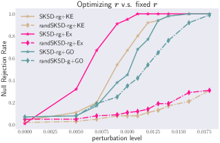
Figure 5: The test power difference with good $\bm{r}$ and fixed $\bm{r}$.

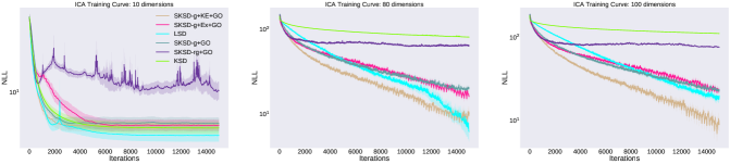
Figure 6: Training curve of ICA model with test NLL for different dimensions.

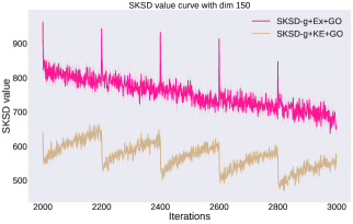
Figure 7: SKSD value curve with 150 dimensional ICA during iteration 5000 to 6000

For all experiments in this paper, we use RBF kernel with median heuristics.

H.1 Benchmark GOF test

For gradient based optimization, we use Adam (Kingma & Ba, 2014) with learning rate $0.001$ and $\beta=(0.9,0.99)$. We use random initialization for SKSD-g+GO by drawing $\bm{g}_{r}$ from a Gaussian distribution before normalizing them to unit vectors. For kernel smooth and gradient estimator, we use RBF kernel with median heuristics. Although the algorithm 1 states that small Gaussian noise are needed for active slices, in practice, we found that active slices still have the satisfactory performance without the noise.

The significance level for GOF test $\alpha=0.05$, and the dimensions of the benchmark problems grow from $2$ to 100. We use $1000$ bootstrap samples to estimate the threshold and run $100$ trials for each benchmark problems.

H.2 RBM GOF test

We set significance level $\alpha=0.05$ and use $1000$ bootstrap samples to compute the threshold. For methods that require training (SKSD based method), we need to collect some training samples. Following the same settings as (Gong et al., 2021), to avoid over-fitting to small training set, we collect the pseudo-samples during the early burn-in stage. Note that these pseudo-samples should not be used for testing, as they are not drawn from the $q$. We collect $2000$ samples. For gradient based optimization, we use the same optimizer as benchmark GOF test with the same hyper-parameters. The batch size is 100. For initialization of SKSD+GO, we found that if the slices are initialized randomly, the gradient optimization fails to find meaningful slices within a reasonable amount of time, therefore, we have initialize the $\bm{r}$ and $\bm{g}_{r}$ as one-hot vectors and set $\bm{r}=\bm{g}_{r}$. For pruning ablation study, if the pruning level is set to $50$, we initialize $\bm{r}$ and $\bm{g}_{r}$ to be the identity matrix. The default number of gradient optimization for SKSD+GO is $50$. For active slice method, we directly use the active slices without any further optimizations. We run 100 trials for GOF test with 1000 test samples per trial.

(Gong et al., 2021) reports SKSD-rg+GO has near optimal test power at perturbation level $0.01$. The performance difference is because they train the SKSD-rg with $200$ batch sizes per burn-in step. Namely, the training set size are $200\times 2000=400000$, which is 200 times larger than ours. They also run $2000$ iterations, which is equivalent to $100$ epochs in our settings.

Figure 5 shows the test power difference with optimized $\bm{r}$ and fixed $\bm{r}$. The legend with rand annotation implies we randomly initialized $\bm{r}$ as one-hot vectors and fix them while updating $\bm{g}_{r}$ using GO or active slice. Without rand, it means both $\bm{r}$ and $\bm{g}_{r}$ are optimized. We only use 3 $\bm{r}$ for active slice method and 50 for gradient-based counterpart. For active slice method with pruning (randSKSD-g+Ex or randSKSD-g+KE), despite we show that any finite random slices define a valid discrepancy, it is clear that the performance is quite poor with random initialized $\bm{r}$’s. It indicates that using active slices of $\bm{g}_{r}$ alone cannot compensate the poor discriminating power of the random $\bm{r}$’s. Although SKSD-rg+GO demonstrates an advantage compared to randSKSD-g+GO, the performance boost is less clear compared to active slices method. This is because we do not use any pruning for randSKSD-g+GO, and adopt orthogonal basis $O_{r}=\bm{I}$. Despite the orthogonal basis may not capture the important directions, they can provide reasonable discriminating power due to their orthogonality from each other. In summary, using good directions for $\bm{r}$ is advantageous compared to fixed $\bm{r}$.

H.3 Model learning: Training ICA

We use Adam optimizer for the model and slice directions with learning rate $0.001$ and $\beta=(0.9,0.99)$. We totally run $15000$ iterations. The batch size is 100. We evaluate our method in dimension 10, 80, 100 and 150. For more stable comparisons, we initialized the weight matrix $\bm{W}$ until its conditional number is smaller than its dimensions. For active slice method, we use randomly sampled $3000$ data from training set to estimate the score difference and the matrices used for eigen-decomposition.

For SKSD-rg+GO, we initialize the $\bm{r}$ to be a group of one-hot vectors to form identity matrix and $\bm{g}_{r}=\bm{r}$. We use an adversarial training procedure that updates both $\bm{r}$ and $\bm{g}_{r}$ using Adam once per iteration before we update the model. For SKSD-g+GO, we fix the orthogonal basis $O_{r}$ to be the identity matrix and only update $\bm{g}_{r}$. Each results are the average of 5 runs of training.

As for the reason why SKSD-g+Ex+GO performs worse than +KE+GO, we suspect that +Ex only focus on directions with high discriminating power. However, high discriminating power is not necessarily good for model learning. It may focus on very small area that is different from the target but ignore the larger area with small difference. Because our algorithm for finding basis is greedy, this means it can ignore the generally good directions if they are not orthogonal to the directions with high discriminating power.

From figure 7, we can observe there is a spike of SKSD-g+Ex+GO value at every 200 iterations due to the new active slices found at the beginning of each training epoch. However, the value drops significantly fast to the one before new active slices. This indicates the Ex indeed finds directions with large discriminating power but they do not represents good directions for learning due to the fast drop of SKSD values. On the other hand, the directions provided by KE does not give the highest discriminating power, but it can find generally good directions of $\bm{g}_{r}$ using GO refinement steps within a few iterations. This means the directions found by KE indeed represents good directions for learning as the model cannot decrease this value quickly. We guess this is due to the smooth estimation of KE, where very small areas with high discriminating power are smoothed out.

Figure 6 shows the ICA training curve of other dimensions. We can observe the convergence speed of LSD deteriorates as the dimension increases due to the poor test function in early training stage, whereas SKSD-g+KE+GO maintains the fastest convergence in high dimensions.

Appendix I Perturbation of eigenvectors

The active slice method (algorithm 1) is mainly based on the eigenvalue-decomposition of matrix $\boldsymbol{H}$, where

$$\boldsymbol{H}=\int q(\boldsymbol{x})\nabla_{\boldsymbol{x}}f_{r}^{*}(\boldsymbol{x})\nabla_{\boldsymbol{x}}f_{r}^{*}(\boldsymbol{x})^{T}d\boldsymbol{x}$$

Obtaining the analytic form of $\boldsymbol{H}$ involves complicated integration, so Monte Carlo estimation is often used for approximation. We denote it as $\hat{\boldsymbol{H}}$, with M being the number of samples:

$$\hat{\boldsymbol{H}}=\frac{1}{M}\sum_{i=1}^{M}[\nabla_{\boldsymbol{x}_{i}}f_{r}^{*}(\boldsymbol{x}_{i})\nabla_{\boldsymbol{x}_{i}}f_{r}^{*}(\boldsymbol{x}_{i})^{T}]$$ (53)

Let $\boldsymbol{g}$ be the top eigenvector of $\boldsymbol{H}$ and $\hat{\boldsymbol{g}}$ be the top eigenvector of $\hat{\boldsymbol{H}}$. Let $\lambda_{1}$, $\lambda_{2}$ be the top two eigenvalues of $\boldsymbol{H}$. Assuming the error matrix $\boldsymbol{E}=\hat{\boldsymbol{H}}-\boldsymbol{H}$ is deterministic, (Yu et al., 2015) proved that

$$||\boldsymbol{g}\boldsymbol{g}^{T}(\boldsymbol{I}-\hat{\boldsymbol{g}}\hat{\boldsymbol{g}}^{T})||_{F}\leq\frac{2||\boldsymbol{E}||_{op}}{\lambda_{1}-\lambda_{2}}$$ (54)

where we define the operator norm for a given $n\times n$ matrix $\boldsymbol{A}$ as

$$||\boldsymbol{A}||_{op}=\sup\{||\boldsymbol{A}\boldsymbol{x}||:x\in\mathbb{R}^{n}\ \text{with}\ ||\boldsymbol{x}||=1\}$$

We also have (with proof below)

$$\min_{\epsilon\in\{-1,1\}}||\boldsymbol{g}-\epsilon\hat{\boldsymbol{g}}||_{2}\leq\sqrt{2}||\boldsymbol{g}\boldsymbol{g}^{T}(\boldsymbol{I}-\hat{\boldsymbol{g}}\hat{\boldsymbol{g}}^{T})||_{F}$$ (55)

Inequality 54 and 55 imply that,

$$\min_{\epsilon\in\{-1,1\}}||\boldsymbol{g}-\epsilon\hat{\boldsymbol{g}}||_{2}\leq 2^{3/2}\frac{||\hat{\boldsymbol{H}}-\boldsymbol{H}||_{op}}{\lambda_{1}-\lambda_{2}}$$ (56)

I.1 Proof of inequality 55

Proposition 5.

Let $\bm{S}$ and $\bm{U}$ be two matrices with orthonormal columns and equal rank $r$. Let $\bm{\Pi}_{S}$ ($resp.$ $\bm{\Pi}_{U}$) indicates the projection matrix to the column space of $\bm{S}$ ($resp.$ $\bm{U}$). Then

$$\min_{O\in\mathbb{R}^{r\times r}\operatorname{orthogonal}}||\bm{S}-\bm{U}\bm{O}||_{F}\leq\sqrt{2}||\bm{\Pi}_{S}(\bm{I}-\bm{\Pi}_{U})||_{F}$$ (57)

When $r=1$, we denote $\boldsymbol{O}$ as $\epsilon$. Following the definition of orthogonal matrix, we have $\epsilon^{T}\epsilon=\epsilon^{2}=1$, hence $\epsilon\in\{-1,1\}$. Substituting $\bm{S}=\boldsymbol{g}$ and $\boldsymbol{U}=\hat{\boldsymbol{g}}$, we get inequality 55.

Proof.

Let $\bm{W}\bm{\Sigma}\bm{V}^{T}$ be a singular value decomposition of $\bm{S}^{T}\bm{U}$, and use $\bm{O}=\bm{V}\bm{W}^{T}$.Now,

$$||\bm{S}-\bm{U}\bm{O}||^{2}_{F} =\operatorname{Tr}((\bm{S}-\bm{U}\bm{O})^{T}(\bm{S}-\bm{U}\bm{O}))$$

$$=||\bm{S}||^{2}_{F}+||\bm{U}||^{2}_{F}-2\operatorname{Tr}(\bm{O}\bm{S}^{T}\bm{U})$$

$$=2r-2\operatorname{Tr}(\bm{\Sigma})$$

where r is the rank of $\bm{S}$ and $\bm{U}$. On the other hand, by Pythagora’s theorem

$$||\bm{\Pi}_{S}(\bm{I}-\bm{\Pi}_{U})||_{F}^{2} =||\bm{\Pi}_{S}||_{F}^{2}-||\bm{\Pi}_{S}\bm{\Pi}_{U}||_{F}^{2}$$

$$=r-||\bm{\Pi}_{S}\bm{\Pi}_{U}||_{F}^{2}$$

$$=r-||\bm{SS}^{T}\bm{UU}^{T}||_{F}^{2}$$

$$=r-\operatorname{Tr}(\bm{\Sigma}^{2})$$

We claim that the entries of $\bm{\Sigma}$ are bounded above by 1, such that $\operatorname{Tr}(\bm{\Sigma})\leq\operatorname{Tr}(\bm{\Sigma}^{2})$, then

$$\min_{O\in\mathbb{R}^{r\times r}\operatorname{orthogonal}}||\bm{S}-\bm{U}\bm{O}||_{F}^{2} \leq 2r-2\operatorname{Tr}(\bm{\Sigma})$$

$$\leq 2r-2\operatorname{Tr}(\bm{\Sigma}^{2})$$

$$=2||\bm{\Pi}_{S}(\bm{I}-\bm{\Pi}_{U})||_{F}^{2}$$

Taking the square root of both sides yields the desired inequality. To prove the claim, let $\bm{\omega}=[\bm{S},\bm{S}^{\prime}]$ and $\tilde{\bm{U}}=[\bm{U},\bm{U}^{\prime}]$ be orthogonal matrices. Then $\bm{S}^{T}\bm{U}$ is a diagonal block in $\bm{\omega}^{T}\tilde{\bm{U}}$. It follows that $\max_{i}\Sigma_{i,i}=||\bm{S}^{T}\bm{U}||_{op}\leq||\bm{\omega}^{T}\tilde{\bm{U}}||_{op}=1$ ∎

From Eq.56, we can see if the top two eigenvalues are similar, then their corresponding eigenvectors can be arbitrary different. In terms of our active slice algorithm, it means if the most discriminating directions for two distributions $q$, $p$ have similar ”magnitude of difference”, our algorithm may fail under Monte-carlo approximation. On the other hand, if the eigenvalues are different, Eq.56 guarantees that eigenvectors from $\hat{\bm{H}}$ are not far-away from the truth.

References

- Arcones & Gine (1992) Arcones, M. A. and Gine, E. On the bootstrap of u and v statistics. The Annals of Statistics, pp. 655–674, 1992.
- Ceylan & Gutmann (2018) Ceylan, C. and Gutmann, M. U. Conditional noise-contrastive estimation of unnormalised models. In International Conference on Machine Learning, pp. 726–734. PMLR, 2018.
- Chen et al. (2019) Chen, P., Wu, K., Chen, J., O’Leary-Roseberry, T., and Ghattas, O. Projected stein variational newton: A fast and scalable bayesian inference method in high dimensions. arXiv preprint arXiv:1901.08659, 2019.