Constant mean curvature surfaces based on fundamental quadrilaterals

Abstract.

We describe the construction of CMC surfaces with symmetries in $\mathbb{S}^{3}$ and $\mathbb{R}^{3}$ using a CMC quadrilateral in a fundamental tetrahedron of a tessellation of the space. The fundamental piece is constructed by the generalized Weierstrass representation using a geometric flow on the space of potentials.

Introduction

Surfaces with constant mean curvature (CMC) in euclidean 3-space and in the round 3-sphere can be investigated by methods of integrable systems. Their Gauss equation is the elliptic sinh-Gordon equation

(0.1) $$\Delta u+\sinh u=0\,\,\,,$$

which is one of the basic examples of integrable equations. Similar to minimal surfaces in euclidean 3-space, CMC surfaces possess 1-parameter (denoted usually by $\lambda$) families of isometric associated surfaces obtained by rotating their Hopf differential. This allows CMC surfaces to be described in terms of loop groups [4], so that analytic methods of the theory of integrable systems can be applied. One of the powerful methods of the construction of CMC surfaces is the generalized Weierstrass representation (DPW) by Dorfmeister-Pedit-Wu [6]. It starts with an analytic differential equation for the holomorphic frame $\Phi_{z}=\Phi\xi$ with a meromorphic DPW potential $\xi(z,\lambda)$ and the subsequent loop group factorization of $\Phi$, leading to immersion formulas for the CMC surfaces. Control of the monodromy of the holomorphic frame is of crucial importance for the construction of CMC surfaces with non-trivial topology and symmetries.

16cm(14.5cm,7.5cm)

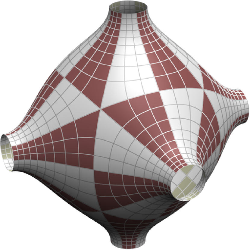
(a) cube (bulge)

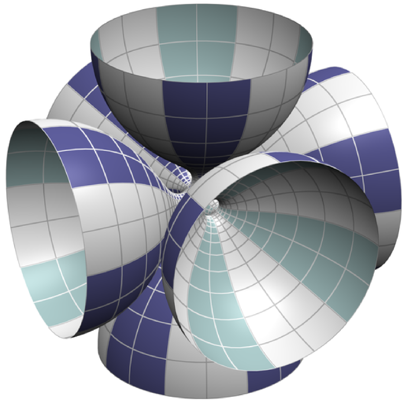
(b) cube (neck)

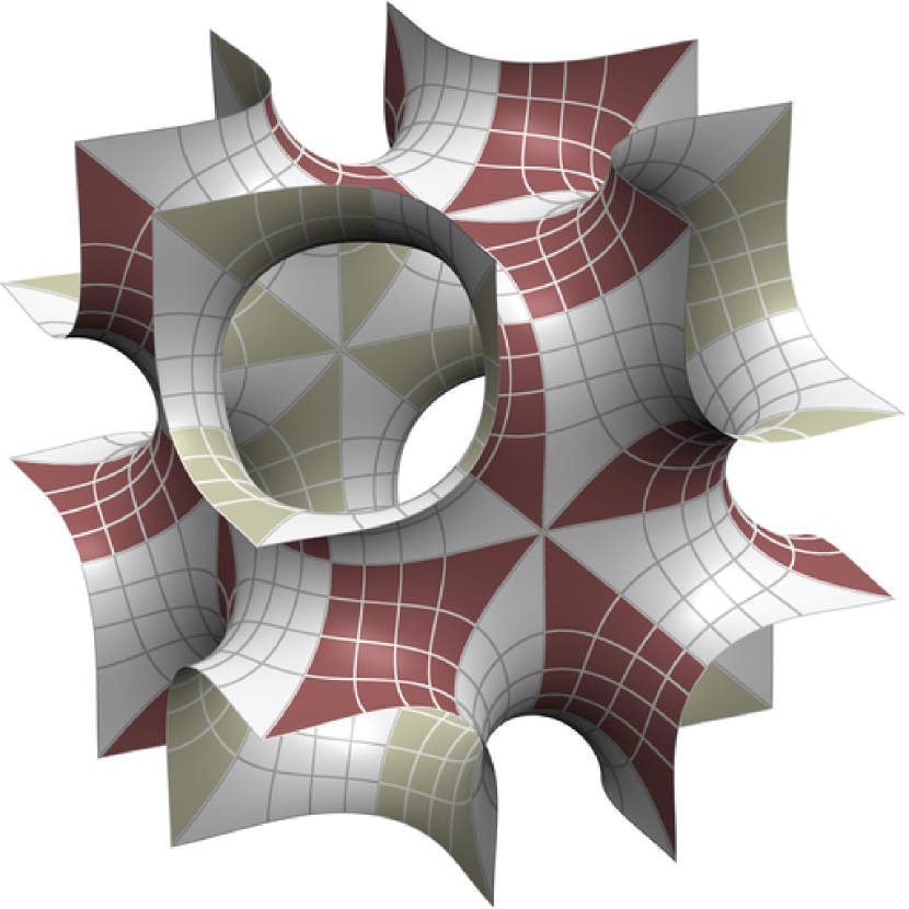
(c) octahedron

Figure 1. Triply periodic CMC surfaces in $\mathbb{R}^{3}$

A particularly important class of potentials is given by Fuchsian systems $\xi(z)$, those with only simple poles. In the simplest case of three singularities it reduces to the hypergeometric equation (see, for example, [7]), whose monodromy group can be described explicitly from the local residues. This leads to CMC surfaces based on fundamental triangles [25]. From the geometric point of view, CMC surfaces constructed from fundamental quadrilaterals are more natural, since they come from the curvature line parametrization. But for Fuchsian systems with more then three singularities the monodromy cannot be computed explicitly in terms of the coefficients of the system, introducing accessory parameters. Then the simplest holomorphic frame equation is a Fuchsian system with four singularities on the Riemann sphere

(0.2) $$\Phi_{z}=\Phi\sum_{k=0}^{3}\frac{A_{k}}{z-z_{k}}\,\,\,.$$

In section 4 of this paper we show how all periodic and compact surfaces based on fundamental quadrilaterals can be constructed from the system (0.2). Our constructions make explicit use of this Fuchsian DPW form. The relation of the monodromy and the coefficients of the Fuchsian system is the famous Hilbert’s 21st problem, which was intensely studied [1]. There exist many important partial results in the simplest non-trivial case of four singularities. This case was investigated mostly within the theory of isomonodromic deformations [7] and the Painlevé VI equation, where the problem is to describe the coefficients $A_{k}$ as functions of the poles $z_{j}$ when the monodromy group is preserved. The holomorphic frame $\Phi(z,\lambda)$ of a CMC surface lies in a loop group, and the main analytic problem is to construct solutions whose monodromy group is unitary on the unit circle $|\lambda|=1$, giving global solutions of the Gauss equation on the four-punctured sphere.

In general, it is a hard problem to control the intrinsic and extrinsic closing conditions to obtain closed surfaces or surfaces with prescribed global properties. In recent years, important progress has been made using a flow of DPW potentials [27, 28, 13] or similar methods on spectral data [12]. By the very nature of these techniques, only surfaces which are small perturbations of spheres or tori have been reached [13].

16cm(14.5cm,5cm)

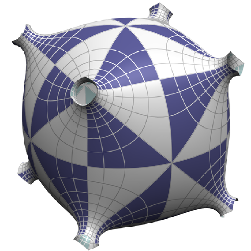
(a) alternate octahedron

(b) alternate octahedron

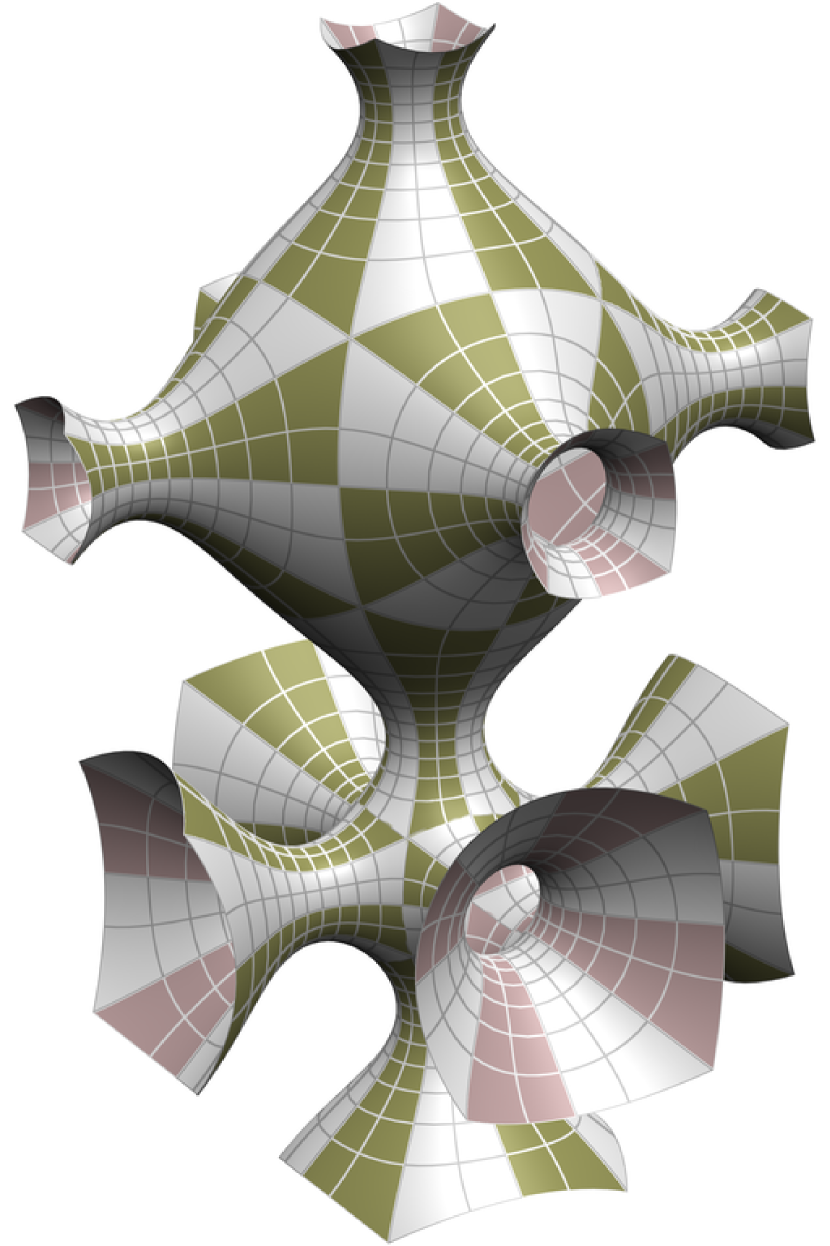
(c) alternate cube

Figure 2. Triply periodic CMC surfaces in $\mathbb{R}^{3}$

In [18] Lawson constructed the first compact minimal surfaces in the round 3-sphere of genus $g\geq 2.$ A fundamental piece of a Lawson surface is obtained by the Plateau solution of a specific geodesic polygon. The compact surface is then built from the fundamental 4-gon by the finite group generated by rotations around the geodesic edges of the polygon. Later, Karcher-Pinkall-Sterling [16] constructed new minimal surfaces in the 3-sphere by starting with a tessellation of the 3-sphere into tetrahedra. The minimal surfaces are obtained from fundamental minimal 4-gons within such a tetrahedron which reflect across the geodesic boundaries. Constant mean curvature (CMC) surfaces in $\mathbb{R}^{3}$ have been constructed by adapting these methods [8]; see also [22, 10] for related computer experiments.

This paper constructs such fundamental patches of surfaces (section 3) based on the deformation of DPW potentials. In this paper the following new surfaces are numerically constructed: triply periodic surfaces (figure 1b-c, figure 2) and doubly periodic surfaces (figure 3b-c, figure 4b-c, figure 5b-c), new doubly periodic surfaces with Delaunay ends (figure 11), new surfaces with Delaunay ends of positive genus (figures 22, 23 and 30) as well as new KPS-type surfaces (figure 27a,d). We also reconstruct by these methods previously constructed surfaces based on doubly-periodic hexagonal, square and triangular tilings of the plane, triply periodic cubic examples, cylinders with ends [8, 9], and the Lawson and KPS surfaces [18, 16].

The 3D-data of the surfaces constructed in this paper are available in the DGD Gallery [5].

1. Geometric construction

1.1. The construction

This report reports on the experimental construction of CMC surfaces in $\mathbb{R}^{3}$ with genus with and without Delaunay ends via the generalized Weierstrass representation (DPW) [6]. The construction starts with a tetrahedron in $\mathbb{R}^{3}$ as shown which tessellates $\mathbb{R}^{3}$ by the group generated by the reflections in the four planes containing its faces. Each of the six edges of the tetrahedron is marked with an integer $n\in\mathbb{N}_{\geq 1}\cup\{\infty\}$ specifying that the internal dihedral angle between the two planes meeting at that edge is $\pi/n$. The tetrahedron can be degenerate in the following ways:

• vertex at $\infty$

• parallel planes, with opposite outward normals: the edge of the tetrahedron between the two planes is marked with $\infty$

• coincident planes, with the same outward normal: the edge of the tetrahedron between the two planes is marked with $1$.

In this tetrahedron construct a CMC quadrilateral as shown, such that

• each of the four edges of the quadrilateral lies in a plane of the tetrahedron, and the surface reflects smoothly across this plane

• at each of the four vertices of the quadrilateral, application of the tessellation group results in a surface with either an immersed point of the surface or a once-wrapped Delaunay end at the vertex.

Then the surface constructed by application of the tessellation group is a CMC immersion with optional Delaunay ends and the symmetries of that group. Its genus is finite if the tessellation group is finite, and infinite if the group is infinite. These surfaces are described in detail at the end of this section.

The polygon is constructed via a Fuchsian DPW potential on $\mathbb{C}\mathrm{P}^{1}$ with four simple poles on $\mathbb{S}^{1}$ (section 3.1) and a reflection symmetry across $\mathbb{S}^{1}$. The unit disk is the domain of a CMC quadrilateral which reflects in planes containing its boundaries. The simple poles with constant or Delaunay residue eigenvalues insure that each vertex of the quadrilateral after reflection is either immersed or a Delaunay end. The four dihedral angles of the tetrahedron at the corners of the quadrilateral are controlled by the four local monodromies of the potential, and the two remaining dihedral angles by two global monodromies.

The potential has two accessory parameters which are computed by the unitary flow (section 3.3). Starting with an initial surface (section 3.2) which satisfies the intrinsic closing condition (unitary monodromy on $\mathbb{S}^{1}_{\lambda}$), the unitary flow, which preserves this condition, is run through the space of potentials until the dihedral angles of the planes reach the values prescribed by the tessellation. The dihedral angles are controlled by certain monodromy traces at the evaluation point. The unitary flow is not known in general to exist, but short time existence can be shown in some cases [12]. Hence we construct the surfaces numerically, giving evidence that the unitary flow has long time existence.

The Lawson surfaces [18] (figure 25) and the surfaces of Karcher-Pinkall-Sterling [16] (figures 26 and 27 and figures 28 and 29) have been constructed by solutions of Plateau problems. The cubic lattice and some of the 2-dimensional lattices were shown to exist by similar methods [8].

1.2. Tetrahedral tessellations

The following theorem classifies the tetrahedral tessellation of $\mathbb{S}^{3}$ (which are compact) and of $\mathbb{R}^{3}$ (which are compact, paracompact or degenerate). The tetrahedral tessellation of $\mathbb{H}^{3}$, which can be determined by the same methods, are omitted for simplicity.

16cm(14.5cm,7.5cm)

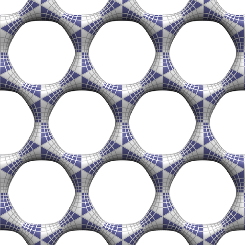
(a) hexagon (bulge)

(b) hexagon (neck)

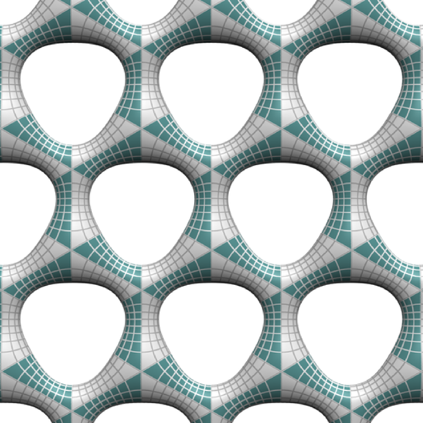
(c) alternate hexagon

Figure 3. Doubly periodic CMC surfaces in $\mathbb{R}^{3}$

Theorem 1.1.

1. The tetrahedral tessellations of $\mathbb{S}^{3}$ are as follows:

      $$a,\,b\in\mathbb{N}_{\geq 2}$$ Minimal Lawson surfaces

      surfaces with respective tetrahedral, octahedral, and icosahedral symmetries

      surfaces with respective -cell, /-cell and /-cell symmetries

   surface with -cell symmetry

   subgroup of -cell

2. The tetrahedral tessellations of $\mathbb{R}^{3}$ are as follows:

         triply periodic surfaces

      $$(a,\,b,\,c)$$ one of , or doubly periodic surfaces

      singly periodic surfaces

      a permutation of , or surfaces with Platonic symmetries and Delaunay ends

      a permutation of , or

         tori with Delaunay ends

        

   

Proof.

Necessary conditions that a compact tetrahedron tessellates one of the spaceforms $\mathbb{S}^{3}$, $\mathbb{R}^{3}$ or $\mathbb{H}^{3}$ are the following.

• Each edge of the tetrahedron is marked with an integer $n\in\mathbb{N}_{\geq 2}$ denoting that the internal dihedral angle between the two faces meeting at that edge is $\pi/n$.

• At each vertex of the tetrahedron, the three integers marking the three edges meeting at the vertex are $(2,\,2,\,n)$, $n\in\mathbb{N}_{\geq 2}$ or $(2,\,3,\,k)$, $k\in\{3,\,4,\,5\}$.

• The Gram matrix $T\in{\mathrm{M}}_{n\times n}{(}\mathbb{R})$ defined by $T_{ij}=-\cos\pi/n_{ij}$ has signature $(\delta,\,1,\,1,\,1)$, where $\delta=1$, $0$ or $-1$ for $\mathbb{S}^{3}$, $\mathbb{R}^{3}$ and $\mathbb{H}^{3}$ respectively.

16cm(14.5cm,7.5cm)

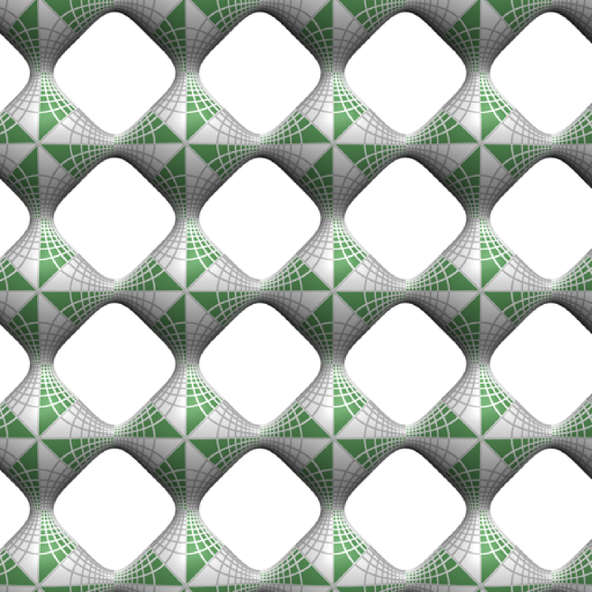
(a) square (bulge)

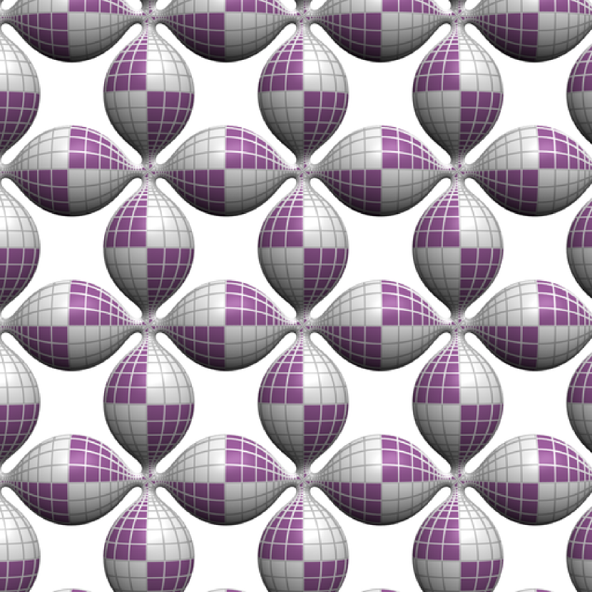
(b) square (neck)

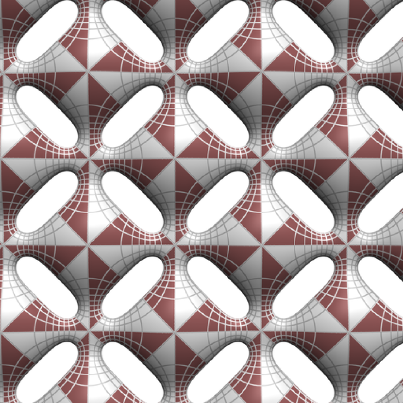
(c) alternate square

Figure 4. Doubly periodic CMC surfaces in $\mathbb{R}^{3}$

The compact tetrahedra in $\mathbb{S}^{3}$, $\mathbb{R}^{3}$ and $\mathbb{H}^{3}$ are the following:

$$\begin{array}[]{c}\includegraphics{diagram/tet-c-compact-A.pdf}\\ \text{\tiny$a,b\in\mathbb{N}_{\geq 2}$}\\ A_{ab}\end{array}\quad\begin{array}[]{c}\includegraphics{diagram/tet-c-compact-B.pdf}\\ \text{\tiny$a,b\in\{2,3,4,5\}$}\\ B_{ab}\end{array}\quad\begin{array}[]{c}\includegraphics{diagram/tet-c-compact-C.pdf}\\ \text{\tiny$a\in\{2,3,4,5\}$}\\ C_{a}\end{array}\quad\begin{array}[]{c}\includegraphics{diagram/tet-c-compact-D.pdf}\\ \text{\tiny$a,b\in\{2,3,4,5\}$}\\ D_{ab}\end{array}$$

with identifications $A_{ba}=A_{ab}$, $B_{ba}=B_{ab}$, $D_{ba}=D_{ab}$ and

(1.1) $$A_{23}=B_{22}\,\,\,,\quad A_{33}=D_{22}\,\,\,,\quad B_{23}=C_{2}\,\,\,,\quad B_{33}=D_{23}\,\,\,.$$

To see this, first consider those tetrahedra with at least one edge marked with $4$ or $5$. Then at each of the vertices at the endpoints of that edge, the other two edges meeting the vertex must be marked with $2$ and $3$. Hence all such tetrahedra with at least one $4$ or $5$ is one of the four types $A_{ab}$, $B_{ab}$, $C_{a}$ or $D_{ab}$. The remaining tetrahedra have only $2$ or $3$ at each face. There are seven of these, namely $A_{22}$, $A_{23}=B_{22}$, $B_{23}=C_{2}$, $C_{3}$, $A_{33}=D_{22}$, $B_{33}=D_{23}$ and $D_{33}$.

Since its Gram matrix has positive determinant, the tetrahedron $A_{ab}$ is in $\mathbb{S}^{3}$. The spaceforms for the other tetrahedra $B_{ab}$, $C_{a}$ and $D_{ab}$ are determined by the signs of the determinate of the Gram matrix as follows:

(1.2) $$\small\begin{array}[t]{c|cccc}B&2&3&4&5\\ \hline\cr 2&[+]&+&+&+\\ 3&&+&+&+\\ 4&&&0&-\\ 5&&&&-\end{array}\qquad\begin{array}[t]{c|cccc}C&2&3&4&5\\ \hline\cr&[+]&+&0&-\end{array}\qquad\begin{array}[t]{c|cccc}D&2&3&4&5\\ \hline\cr 2&[+]&[+]&+&-\\ 3&&0&-&-\\ 4&&&-&-\\ 5&&&&-\end{array}$$

The $[+]$ in the above tables denotes entries which are redundant due to the identifications (1.1)

Hence the tetrahedra which tessellate $\mathbb{S}^{3}$ are $A_{ab}$ and the seven tetrahedra $B_{23}$, $B_{24}$, $B_{25}$, $B_{33}$, $B_{34}$, $B_{35}$ and $D_{24}$. These tessellate $\mathbb{S}^{3}$ because they tessellate either a sphere or a $n$-cell, which in turn tessellates $\mathbb{S}^{3}$.

The compact tetrahedra which tessellate $\mathbb{R}^{3}$ are the three tetrahedra $B_{44}$, $C_{4}$ and $D_{33}$. The first two tessellate a cube and the third tessellates a rhombic dodecahedron, each of which in turn tessellates $\mathbb{R}^{3}$.

The paracompact tetrahedral tessellations of $\mathbb{R}^{3}$ are classified similarly except that the integer triple at each vertex is as in the compact case or one of $(3,\,3,\,3)$, $(2,\,4,\,4)$ or $(2,\,3,\,6)$.

The degenerate tetrahedral tessellations of $\mathbb{R}^{3}$ are classified similarly except that the integer triple at each vertex is as in the paracompact case or one of $(2,\,2,\,\infty)$ or $(1,\,n,\,n)$, $n\in\mathbb{N}_{\geq 1}\cup\{\infty\}$. ∎

1.3. The surfaces

This section describes the experimentally constructed minimal surfaces in $\mathbb{S}^{3}$ and CMC surfaces in $\mathbb{R}^{3}$. They are of the types:
In $\mathbb{R}^{3}$:

• triply periodic CMC surfaces $\mathbb{R}^{3}$ without ends (figures 1 and 2)

• doubly periodic CMC surfaces $\mathbb{R}^{3}$ without ends (e.g. figure 3)

• doubly periodic CMC surfaces $\mathbb{R}^{3}$ with ends (figure 11)

• single periodic CMC surfaces in $\mathbb{R}^{3}$ with Delaunay ends (cylinders, figure 16)

• CMC surfaces in $\mathbb{R}^{3}$ with dihedral symmetry and Delaunay ends (tori, figures 19 and 20)

• CMC surfaces in $\mathbb{R}^{3}$ with Platonic symmetries and Delaunay ends (figures 22 and 23)

• CMC spheres in $\mathbb{R}^{3}$ with four Delaunay ends (fournoids, figure 24).

In $\mathbb{S}^{3}$:

• Lawson surfaces $\xi_{ab}$ in $\mathbb{S}^{3}$ (figure 25)

• minimal surfaces in $\mathbb{S}^{3}$ with Platonic symmetries (figures 26 and 27)

• minimal surfaces in $\mathbb{S}^{3}$ with $n$-cell symmetries (figures 28 and 29)

• minimal tori in $\mathbb{S}^{3}$ with Delaunay ends (figure 30).

In all shown figures the lines on the surfaces are curvature lines. The surfaces in $\mathbb{S}^{3}$ are stereographically projected to $\mathbb{R}^{3}$.

16cm(14.5cm,7.5cm)

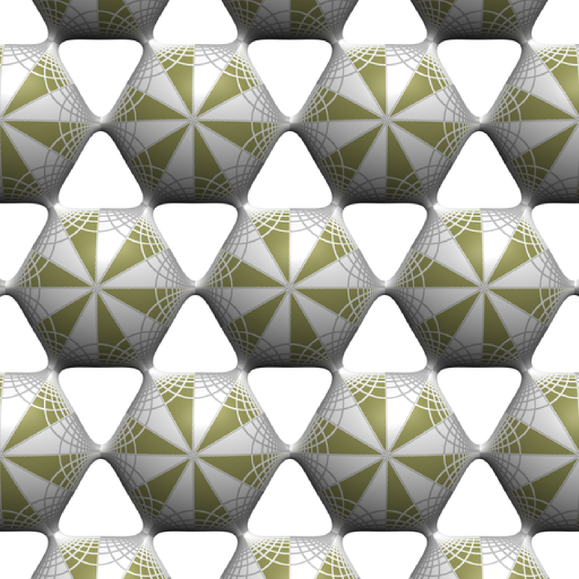
(a) triangle (bulge)

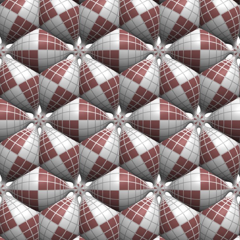
(b) triangle (neck)

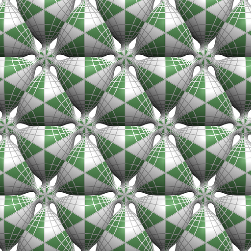
(c) rhombus

Figure 5. Doubly periodic CMC surfaces in $\mathbb{R}^{3}$

Triply periodic surfaces in $\mathbb{R}^{3}$.

The simplest triply periodic surfaces can be thought of as tubes along the edges of the standard cubic lattice in $\mathbb{R}^{3}$ (figure 7). The genus of those surfaces modulo translation is $3$.

The triply periodic surfaces are constructed from the three compact tetrahedra which tessellate $\mathbb{R}^{3}$. Since the CMC quadrilateral can be situated in each tetrahedron in three ways, this gives nine different configurations, of which two are redundant due to symmetry (figure 6).

cube $a_{1}$    oct $a_{2}$    $a_{3}$

alt cube $b_{1}$    alt oct $b_{2}$

$c_{1}$    $c_{2}$

Figure 6. The tetrahedra for the seven possible triply periodic examples.

Of these, $a_{3}$ and $b_{2}$ are not possible under our symmetry constraints (compare with (3.2)), $c_{1}$ seems to devolve to $a_{1}$, and the flow for $c_{2}$ degenerates (figures 1 and 2).

Figure 7. The simplest triply periodic surface and its tetrahedron.

Doubly periodic surfaces in $\mathbb{R}^{3}$.

The doubly periodic surfaces can be thought of as tubes along the edges of a triangle tessellations of $\mathbb{R}^{2}$. The six 2-dimensional lattices are constructed with the tetrahedron below where $(a,\,b,\,c)$ are the indices of a triangle tessellation of $\mathbb{R}^{2}$, that is, a permutation of $(3,\,3,\,3)$, $(2,\,4,\,4)$ or $(2,\,3,\,6)$ (figures 3, 4 and 5).

     lattice (a, b, c) genus hexagon (2, 3, 6) 2 square (2, 3, 6) 2 triangle (2, 3, 6) 3 alt hexagon (3, 3, 3) 2 alt square (4, 4, 2) 2 rhombus (3, 6, 2) 2     

Figure 8. Left: tetrahedron for doubly periodic surface,, where $(a,\,b,\,c)$ is a permutation of $(3,\,3,\,3)$, $(2,\,3,\,6)$ or $(2,\,4,\,4)$. Middle: table of 2-dimensional lattices. The genus listed in the table is that of the surface modulo translations. Right: fundamental piece for a 2-dimensional lattice.

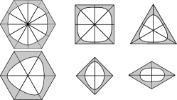
Figure 9. The six $2$-dimensional lattices.

Doubly periodic surfaces in $\mathbb{R}^{3}$ with Delaunay ends. The doubly periodic surfaces with Delaunay ends are obtained from triangle tessellations of $\mathbb{R}^{2}$. Additional freedom is given by the choice of vertices corresponding to Delaunay ends (figure 11).

Cylinders in $\mathbb{R}^{3}$ with ends. Cylinders with Delaunay ends can be constructed from a degenerate tetrahedron with two parallel planes. Of course, the same construction without Delaunay ends give the classical rotational symmetric periodic surfaces, i.e., Delaunay cylinders (figure 16).

Tori in $\mathbb{R}^{3}$ with Delaunay ends. The torus with $n$ ends is constructed via the diagram below (figures 19 and 20). For large $n$, existence of those tori can be shown by growing Delaunay ends in equidistance on one side of a cylinder.

      

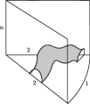
Figure 10. Left: tetrahedron for a torus in $\mathbb{R}^{3}$ with $n$ Delaunay ends and order $n$ cyclic symmetry and $n$ ends. Right: fundamental piece of this torus.

16cm(14.5cm,13.8cm)

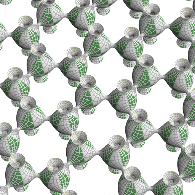
(a) hexagon lattice with ends (bulge)

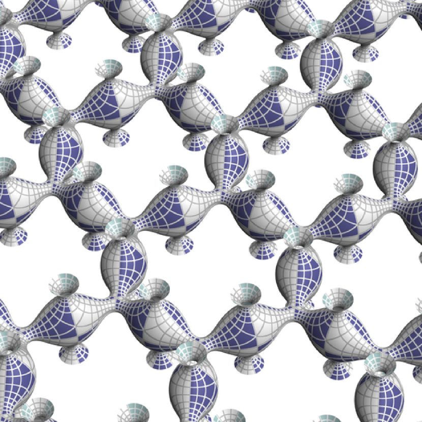
(b) hexagon lattice with ends (neck)

Figure 11. Doubly periodic CMC surfaces in $\mathbb{R}^{3}$ with Delaunay ends

Surfaces in $\mathbb{R}^{3}$ with Platonic symmetry and Delaunay ends.

Given a triangle tessellations of $\mathbb{S}^{2}$, the surface is the orbit of a tube along one edge of the triangle with a Delaunay end at a vertex of the triangle. Equivalently, the surface is built from tubes along the edges of one of the five Platonic solids, with ends emanating from the vertices. The five tetrahedra are as in the diagram below, with $(a,\,b,\,c)$ a permutation of $(2,\,3,\,k)$, $k\in\{3,\,4,\,5\}$ (figures 22 and 23).

   surface (a, b, c) genus tetrahedron (2, 3, 6) 3 octahedron (2, 3, 6) 7 icosahedron (2, 3, 6) 19 cube (2, 3, 6) 5 dodecahedron (2, 3, 6) 11   

Figure 12. Left: Tetrahedron for Platonic surfaces in $\mathbb{R}^{3}$, where $(a,\,b,\,c)$ is a permutation of $(2,\,3,\,k)$. Right: fundamental piece of the surfaces with Platonic symmetry and Delaunay ends.

Lawson surfaces. Classically, the Lawson surfaces [18] are constructed from Plateau solutions of a geodesic polygon by reflection. The tetrahedron $A_{ab}$ and its inscribed fundamental piece admit a rotational order 2 symmetry around a geodesic through the vertices labeled by $a$ and $b$. The geodesic arc is contained in the fundamental piece. This observation relates the original construction with the construction carried out in the present work, see also [16] (figure 25).

Figure 13. Tetrahedron for Lawson surface $\xi_{a-1,b-1}$.

Surfaces in $\mathbb{S}^{3}$ with Platonic symmetries.

Minimal surfaces in $\mathbb{S}^{3}$ with Platonic symmetries have been constructed by Karcher-Pinkall-Sterling [16]. These surfaces can be thought of as tubes along one edge of a triangle which tessellates $\mathbb{S}^{2}$. Note that [16] does not list all possible surfaces, e.g. the alternate octahedron of genus 11 and the alternate icosahedron of genus 29 are missing (figures 26 and 27).

     symmetry genus tetrahedron 3 cube 5 octahedron 7 alt octahedron 11 dodecahedron 11 icosahedron 19 alt icosahedron 29

Figure 14. Left: tetrahedron for surfaces in $\mathbb{S}^{3}$ with Platonic symmetries. Right: table of these surfaces.

Figure 15. Triangle tessellations of $\mathbb{S}^{2}$. Left to right: cyclic of order $5$, dihedral of order $10$, tetrahedral, octahedral and icosahedra.

16cm(14.5cm,7.5cm)

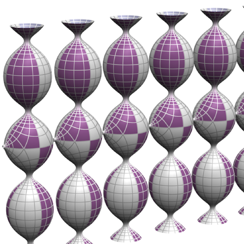
(a) cylinder 2

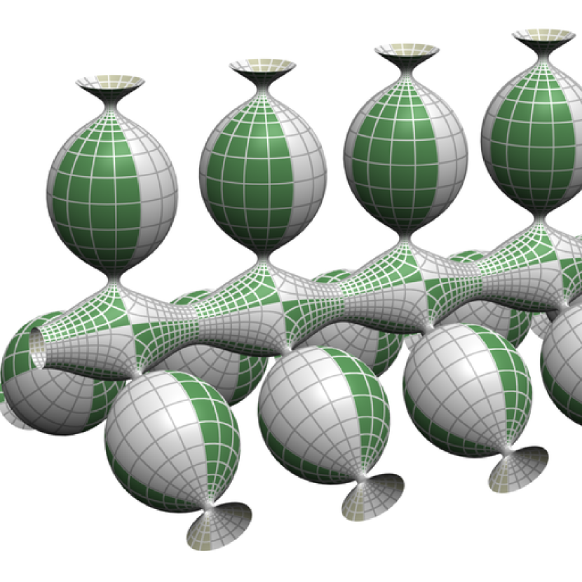
(b) cylinder 3

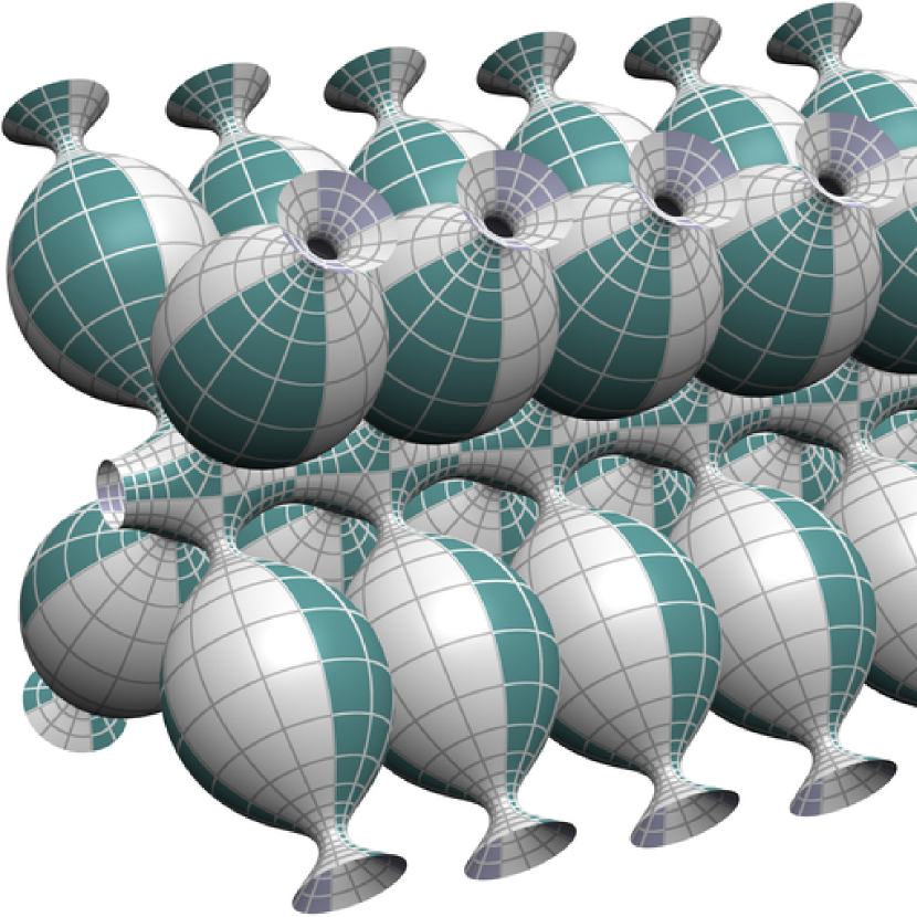
(c) cylinder 4

Figure 16. CMC cylinders in $\mathbb{R}^{3}$ with Delaunay ends

Surfaces in $\mathbb{S}^{3}$ with $n$-cell symmetries.

For each of the $n$-cell tessellations of $\mathbb{S}^{3}$ there is a surface which can be thought of as tubes along the edges of the cells. These minimal surfaces have also been constructed by Karcher-Pinkall-Sterling [16] (figures 28 and 29).

     symmetry genus $5$-cell 6 $16$-cell 17 $24$-cell 73 $600$-cell 601

Figure 17. Left: tetrahedron for surfaces in $\mathbb{S}^{3}$ with $n$-cell symmetries. Right: table of these surfaces.

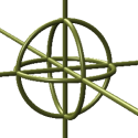
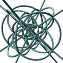
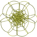
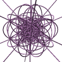
Figure 18. The $5$-, $8$-, $16$-, $24$-, $120$- and $600$-cell tessellations of $\mathbb{S}^{3}$, stereographically projected to $\mathbb{R}^{3}$.

2. CMC polygons via the DPW method

2.1. The generalized Weierstrass representation (DPW)

Define the following loop groups (see [24] for details):

• $\Lambda$ = smooth maps (loops) from $\mathbb{S}^{1}_{\lambda}$ to ${\mathrm{SL}}_{2}{\mathbb{C}}$

• $\Lambda_{u}$ = the subgroup loops in $\Lambda$ which are in ${\mathrm{SU}}_{2}{}$ on $\mathbb{S}^{1}$

• $\Lambda_{+}$ = the subgroup loops in $\Lambda$ which extend to the interior unit disk in $\mathbb{C}\mathrm{P}^{1}_{\lambda}$

• $\Lambda_{-}$ = the subgroup of loops in $\Lambda$ which extend to the exterior unit disk in $\mathbb{C}\mathrm{P}^{1}_{\lambda}$

• $\mathring{\Lambda}_{-}$ = the subgroup of $g\in\Lambda_{\text{--}1}$ such that $g(0)$ is upper triangular with diagonal in $\mathbb{R}^{+}$.

These can be generalized to loops on a circle of radius $r\in(0,\,1)$; see [20].

A DPW potential $\xi$ on a Riemann surface $\Sigma$ is a $\Lambda\mathfrak{sl}({2},\,{\mathbb{C}})$ valued holomorphic differential form on $\Sigma$ with $\xi=\sum_{k=\text{--}1}^{\infty}\xi_{k}\lambda^{k}$, $\det\xi_{\text{--}1}=0$. A meromorphic DPW potential is defined analogously.

A CMC surface is constructed from a DPW potential as follows. Let $\Phi$ be the holomorphic frame solving $\mathrm{d}\Phi=\Phi\xi$; $\Phi$ generally has monodromy. Let $\Phi=FB\in\Lambda_{u}\mathring{\Lambda}_{+}$ be the Iwasawa factorization into the unitary frame $F$ and positive part $B$ (see [24]); for our case of ${\mathrm{SU}}_{2}{}$ this factorization always exists. The CMC surface is constructed via the formulas first obtained in [4]:

(2.1a) $$\mathbb{S}^{3} :\quad f(\lambda_{0},\,\lambda_{1})=F(\lambda_{0})F^{\text{--}1}(\lambda_{1})\,\,\,,\quad\lambda_{0},\,\lambda_{1}\in\mathbb{S}^{1}$$

(2.1b) $$\mathbb{H}^{3} :\quad f(\lambda_{0},\,\lambda_{1})=F(\lambda_{0})F^{\text{--}1}(\lambda_{1})\,\,\,,\quad\lambda_{1}=\lambda_{0}^{\text{--}1}\in\mathbb{C}\setminus\mathbb{S}^{1}$$

(2.1c) $$\mathbb{R}^{3} :\quad f(\lambda_{0})=\text{--}\tfrac{2}{H}\dot{F}(\lambda_{0})F(\lambda_{0})^{\text{--}1}\,\,\,,\quad\lambda_{0}=1\text{ or }\text{--}1$$

where in the case of $\mathbb{R}^{3}$ the dot denotes the derivative with respect to $\theta$, $\lambda=e^{\mathbbm{i}\theta}$. The unitary frame $F$ yields a unitary potential $\mu=F^{-1}\mathrm{d}F$ which is well-defined on the (Riemann) surface as opposed to $F$ which is well-defined only on the universal covering. The unitary potential is also known as the associated family of flat connections, see [14] and the literature therein.

16cm(14.5cm,13.8cm)

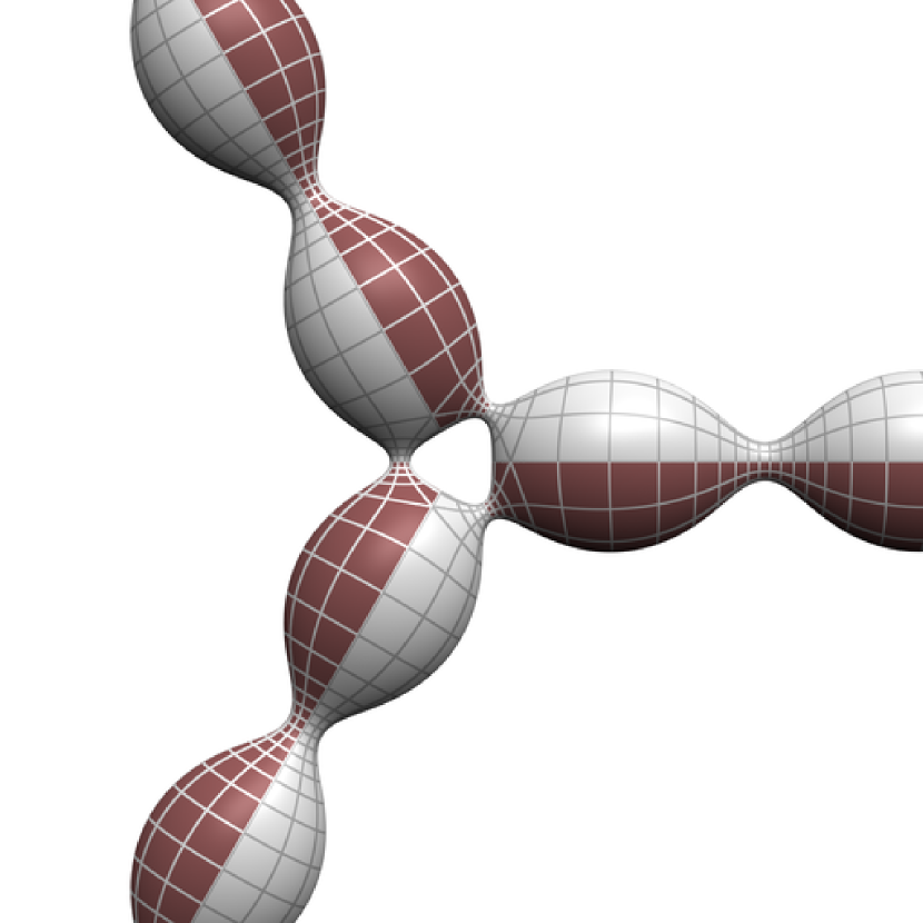
(a) torus 3 (bulge)

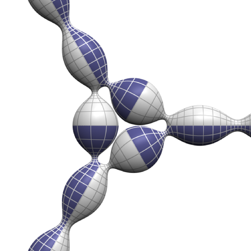
(b) torus 3 (neck)

Figure 19. CMC tori in $\mathbb{R}^{3}$ with Delaunay ends

A DPW potential $\xi=\sum_{k=\text{--}1}^{\infty}\xi_{k}\lambda^{k}$ is adapted if $\xi_{\text{--}1}$ is upper triangular (and hence has zero diagonal because $\det\xi_{\text{--}1}=0$). For adapted DPW potentials, the Hopf differential is $Q=\langle\xi_{\text{--}1},\,\xi_{0}\rangle$. For non-adapted potentials, the formula for $Q$ is more complicated.

If $\xi$ is holomorphic at $z_{0}$, the induced CMC surface is immersed at $z_{0}$ if and only if $\xi_{\text{--}1}$ does not vanish at $z_{0}$.

This representation differs from the original representation [6] in that the potential and loops are not twisted. It is slightly looser than the representation [25] in that it does not require the DPW potential to be adapted.

2.2. Delaunay ends

A Delaunay eigenvalue is

(2.2) $$\nu=\tfrac{1}{2}\sqrt{1+\lambda^{\text{--}1}(\lambda-\lambda_{0})(\lambda-\lambda_{1})w}\,\,\,.$$

where the evaluation points $\lambda_{0}$, $\lambda_{1}$ and the end weight $w\in{\mathbb{R}^{\times}}$ chosen so that $\nu$ is real on $\mathbb{S}^{1}$. A DPW potential with a simple pole, unitary monodromy, and Delaunay eigenvalues of the residue induces a surface asymptotic to a half Delaunay cylinder [17].

To construct surfaces, two types of closing conditions must be satisfied by a DPW potential:

• The intrinsic closing condition is the condition that the monodromy group is unitarizable on $\mathbb{S}^{1}$ (or more generally, $r$-unitarizable on an circle of radius $r\in(0,\,1)$). For the Fuchsian DPW potentials, this condition is not directly satisfiable except in the case of $3$ or $2$ geometric poles; more than $3$ requires the unitary flow, which by definition preserves the intrinsic closing condition.

• The extrinsic closing conditions are conditions on the DPW potential on the monodromy at the evaluation points, chosen to control the desired geometry of the surface via (2.1). For surfaces constructed via tessellations these conditions are given in theorem 2.3.

2.3. Gauge

Consider a holomorphic DPW potential $\xi$ and a holomorphic map $g\colon\Sigma\to\Lambda$. The gauge action is

(2.3) $$\xi\mapsto g^{\text{--}1}\xi g+g^{\text{--}1}\mathrm{d}g\,\,\,.$$

The point of the gauge action is that if $\mathrm{d}\Phi=\Phi\xi$ then $\mathrm{d}(\Phi g)=(\Phi g)({{\xi}{.}{g}})$. We allow gauges to have monodromy $\pm\operatorname{\mathbbm{1}}$ along paths; such multivalued gauges nevertheless map single-values potentials to single-valued potentials.

A DPW gauge is one which maps DPW potentials to DPW potentials, that is, $g\colon\Sigma\to\Lambda_{+}$ is holomorphic in $\lambda$. If $\xi$ is a DPW potential and $g$ is DPW gauge, then $\xi$ and ${{\xi}{.}{g}}$ induce the same surface in the sense that $\Phi$ and $\Phi g$ do. A DPW gauge $g$ is adapted if it preserves adapted DPW potentials, that is, $\left.g\right|_{\lambda=0}$ is upper triangular.

Let $\xi$ be a holomorphic DPW potential on $\Sigma.$ A meromorphic DPW gauge is given by a meromorphic map $g\colon\Sigma\to\Lambda_{+}.$ Then, ${{\xi}{.}{g}}$ is a meromorphic DPW potential with so-called apparent singularities at the singular points of $g$. In general, the singularities of a meromorphic DPW potential are not apparent.

2.4. Spin

For a DPW gauge $g$ define the group homomorphism

(2.4a) $$\operatorname*{spin}:H_{1}(\Sigma)\to\mathbb{Z}_{2}=\{\pm 1\}\,\,\,,$$

(2.4b) $$\operatorname*{spin}_{\gamma}g=\begin{cases}+1&\text{if $g$ has monodromy $+1$ along $\gamma$}\\ -1&\text{if $g$ has monodromy $-1$ along $\gamma$}\end{cases}$$

that is, $\operatorname*{spin}_{\gamma}g=+1$ (resp. $\text{--}1$) if $g$ returns to itself (resp. its negative) along $\gamma$. Then $\operatorname*{spin}_{\gamma}gh=\operatorname*{spin}_{\gamma}g\cdot\operatorname*{spin}_{\gamma}h$.

To define $\operatorname*{spin}$ for DPW potentials consider the double cover

(2.5) $$\mathbb{C}^{2}\setminus\{0\}\to\{x\in\mathfrak{sl}({2},\,{\mathbb{C}})\setminus\{0\}\operatorname{|}\det x=0\}\,\,\,,\quad\bigl{[}\begin{smallmatrix}u\\ v\end{smallmatrix}\bigr{]}\mapsto\bigl{[}\begin{smallmatrix}u\\ v\end{smallmatrix}\bigr{]}\bigl{[}\begin{smallmatrix}\text{--}v&u\end{smallmatrix}\bigr{]}\,\,\,.$$

For a DPW potential $\xi$ on a Riemann surface $\Sigma$, let $\xi_{\text{--}1}$ be its $\lambda^{\text{--}1}$ coefficient. Define the group homomorphism

(2.6a) $$\operatorname*{spin}:H_{1}(\Sigma)\to\mathbb{Z}_{2}=\{\pm 1\}\,\,\,,$$

(2.6b) $$\operatorname*{spin}_{\gamma}\xi=\begin{cases}+1&\text{if the lift of $\xi_{\text{--}1}$ along $\gamma$ is a closed cuvve}\\ -1&\text{otherwise}\end{cases}$$

That is, $\operatorname*{spin}_{\gamma}\xi$ is $+1$ (resp. $\text{--}1$) if the lift of $\xi_{\text{--}1}$ returns to itself (resp. its negative) along $\gamma$. Then $\operatorname*{spin}_{\gamma}{{\xi}{.}{g}}=\operatorname*{spin}_{\gamma}\xi\cdot\operatorname*{spin}_{\gamma}g$.

16cm(14.5cm,7.5cm)

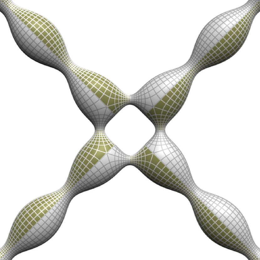
(a) torus 4 (bulge)

(b) torus 6 (bulge)

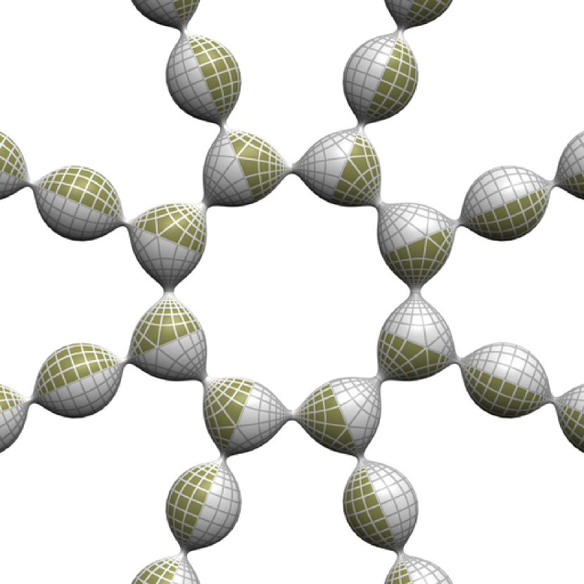
(c) torus 8 (bulge)

Figure 20. CMC tori in $\mathbb{R}^{3}$ with Delaunay ends

The spin can similarly be defined for unitary potentials using the lift of the coefficient of $\lambda^{\text{--}1}$. If $\Phi=FB$ is the holomorphic frame with potential $\xi$, and $F$ is the corresponding unitary frame with potential $\eta$, then $\operatorname*{spin}\eta=\operatorname*{spin}\xi$ because $\operatorname*{spin}B|_{\lambda=0}=1$ since $B|_{\lambda=0}\in\mathring{\Lambda}_{+}$.

A geometric interpretation for the spin of a potential can be given in terms of a coordinate frame, that is, a unitary frame $G$ satisfying

(2.7) $$N=Ge_{0}G^{\text{--}1}\,\,\,,\quad f_{x}/v=Ge_{1}G^{\text{--}1}\,\,\,,\quad f_{y}/v=Ge_{2}G^{\text{--}1}$$

where $e_{0},\,e_{1},\,e_{2}$ is a positively oriented orthonormal basis for $\mathfrak{su}_{2}{}$, $f$ is the CMC immersion, $v$ is the metric of $f$, and $N$ is its normal. Then $\operatorname*{spin}\xi=\operatorname*{spin}u$, where $u=F^{\text{--}1}G$ is the gauge between the unitary frame $F$ and a coordinate frame $G$.

Consider a meromorphic DPW potential $\xi$ on $\Sigma$. For $z\in\Sigma$ write $\operatorname*{spin}_{z}\xi$ to mean $\operatorname*{spin}_{\gamma}\xi$ along a small circle $\gamma$ encircling $z$. If $\xi$ is regular at $z$ then $\operatorname*{spin}_{z}\xi=1.$ For a DPW potential $\xi$ on $\mathbb{C}\mathrm{P}^{1}$ with finitely many singularities we have the total spin

(2.8) $$\prod_{z\in\mathbb{C}\mathrm{P}^{1}}\operatorname*{spin}_{z}\xi=1\,\,\,.$$

As an application of spin, when we construct CMC polygons whose boundaries reflect in planes in section 2.6, the spin is used to distinguish the internal and external dihedral angles of the planes.

2.5. Symmetry

The following theorem and lemma detail how a symmetry of the potential descends to a symmetry of the meromorphic frame, the unitary frame, and the CMC immersion via (2.1).

Theorem 2.1.

Let $\xi$ be a DPW potential.

1. If for a holomorphic automorphism $\tau$ of the domain, $\tau^{\ast}\xi={{\xi}{.}{g}}$, then $\tau^{\ast}\Phi=R\Phi g$ for some $R\in\Lambda$. If $R$ is unitary, then the CMC immersion has the orientation preserving symmetry

   (2.9a) $$\mathbb{S}^{3} \mathbb{H}^{3} :\quad\tau^{\ast}f=RfR^{\text{--}1}$$ and

   (2.9b) $$\mathbb{R}^{3} :\quad\tau^{\ast}f=RfR^{\text{--}1}-\tfrac{2}{H}\dot{R}{R}\,\,\,,$$

   where in the case of $\mathbb{R}^{3}$ the dot denotes the derivative with respect to $\theta$, $\lambda=e^{\mathbbm{i}\theta}$.

2. If for an antiholomorphic automorphism $\tau$ of the domain, $\tau^{\ast}\xi(\lambda)={{\overline{\xi(\overline{\lambda})}}{.}{g}}$, then $\tau^{\ast}\Phi(\lambda)=R\overline{\Phi(\overline{\lambda})}g$ for some $R\in\Lambda$. If $R$ is unitary, then the CMC immersion has the orientation reversing symmetry

   (2.10a) $$\mathbb{S}^{3} \mathbb{H}^{3} :\quad\tau^{\ast}f(\lambda_{0},\,\lambda_{1})=R\overline{f(\overline{\lambda_{0}},\,\overline{\lambda_{1}})}R^{\text{--}1}\,,$$ and

   (2.10b) $$\mathbb{R}^{3} :\quad\tau^{\ast}f(\lambda_{0})=-R\overline{f(\overline{\lambda_{0}})}R^{\text{--}1}-\tfrac{2}{H}\dot{R}{R}\,\,\,.$$

In the orientation reversing case of the above theorem, the symmetry (2.10) relates two associate CMC surfaces, which are the same surface if $\lambda_{1}=\overline{\lambda_{0}}$ (for $\mathbb{S}^{3}$), $\lambda_{0}\in\mathbb{R}$ and $\lambda_{1}\in\mathbb{R}$ (for $\mathbb{H}^{3}$) and $\lambda_{0}\in\{\pm 1\}$ (for $\mathbb{R}^{3}$).

Theorem 2.1 is of limited use without the knowledge that $R$ in that theorem is unitary. One necessary condition that $R$ is unitary is given in the following lemma:

Lemma 2.2.

If $\xi$ in theorem 2.1 extends to $\mathbb{S}^{1}_{\lambda}$ and has irreducible unitary monodromy, then $R$ in that theorem is unitary.

Proof.

Let $f:U\to\Sigma$ be the universal cover, and $\tau$ a lift of $\tau$ to the universal cover, so $f\tau=\tau\circ f$. Let $\sigma$ be a deck transformation, so $f\sigma=f$. Then $f\tau\sigma\tau^{\text{--}1}=f$ implying that $\tau\sigma\tau^{\text{--}1}$ is a deck transformation.

Let $M_{\sigma}$ the monodromy of $\Phi$ with respect to $\sigma$. and $\operatorname*{spin}_{\sigma}\operatorname{\mathbbm{1}}\in\{\pm\operatorname{\mathbbm{1}}\}$ the monodromy of $g$ with respect to $\sigma$. For the orientation reversing case,

(2.11) $$\sigma^{\ast}\tau^{\ast}\Phi=\sigma^{\ast}(R\overline{\Phi}g)=(\operatorname*{spin}_{\sigma}g)R\overline{M}_{\sigma}\overline{\Phi}g=(\operatorname*{spin}_{\sigma}g)R\overline{M}_{\sigma}R^{\text{--}1}\tau^{\ast}\Phi$$

so

(2.12) $${\tau^{\text{--}1}}^{\ast}\sigma^{\ast}\tau^{\ast}\Phi=(\operatorname*{spin}_{\sigma}g)R\overline{M}_{\sigma}R^{\text{--}1}\Phi\,\,\,.$$

Since $\tau\sigma\tau^{\text{--}1}$ is a deck transformation, its monodromy is given by $N_{\sigma}\mathrel{\vbox{\hbox{\scriptsize.}\hbox{\scriptsize.}}}=(\operatorname*{spin}_{\sigma}g)R\overline{M}_{\sigma}R^{\text{--}1}$. Since by assumption the monodromy group is irreducible and unitary, then $N_{\sigma}\in\Lambda_{u}$ for every deck transformation $\sigma$. Using that $\xi$ extends to $\mathbb{S}^{1}_{\lambda}$, this implies $R\in\Lambda_{u}$.

The proof for the orientation preserving case is the same without the overline. ∎

2.6. CMC polygons

Let $\mathbb{R}\cup\{\infty\}$ be divided into $n$ segments $s_{1},\dots,s_{n}$ at $n$ distinct consecutive points $z_{ij}$ dividing $s_{i}$ and $s_{j}$. Let $\xi$ be a meromorphic DPW potential on $\mathbb{C}\mathrm{P}^{1}$ with singularities at these points $z_{ij}$. With $b$ a basepoint in the upper halfplane, for $i,\,j\in\{1,\dots,n\}$ let $\gamma_{ij}$ be a simple closed counterclockwise curve based at $b$ which crosses the segments $s_{i}$ and $s_{j}$, and let $M_{ij}$, $i,\,j\in\{1,\dots,n\}$, $i<j$ be the monodromy along $\gamma_{ij}$. The $n$ local monodromies are those along paths which enclose one singularity; the remaining monodromies are called global.

16cm(14.5cm,7.5cm)

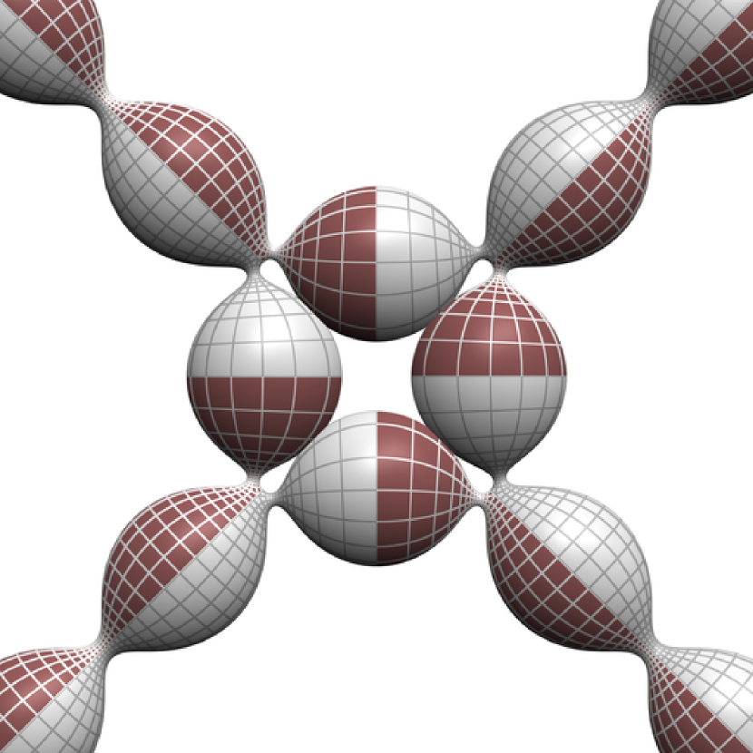
(a) torus 4 (neck)

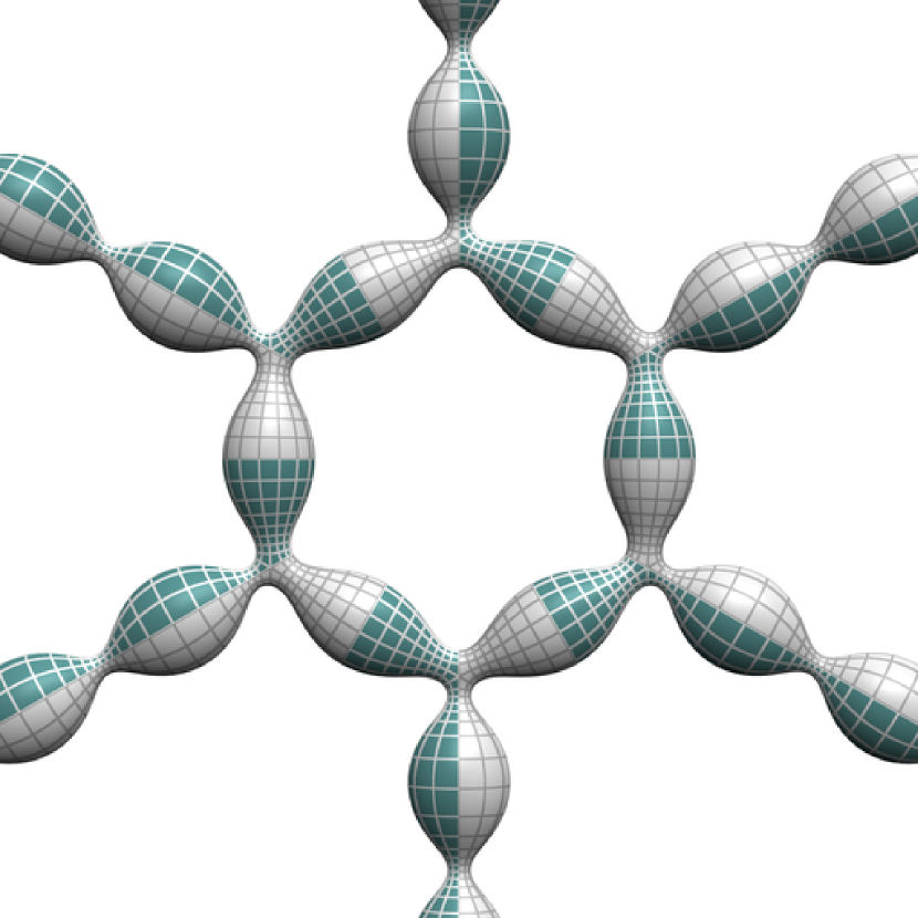
(b) torus 6 (neck)

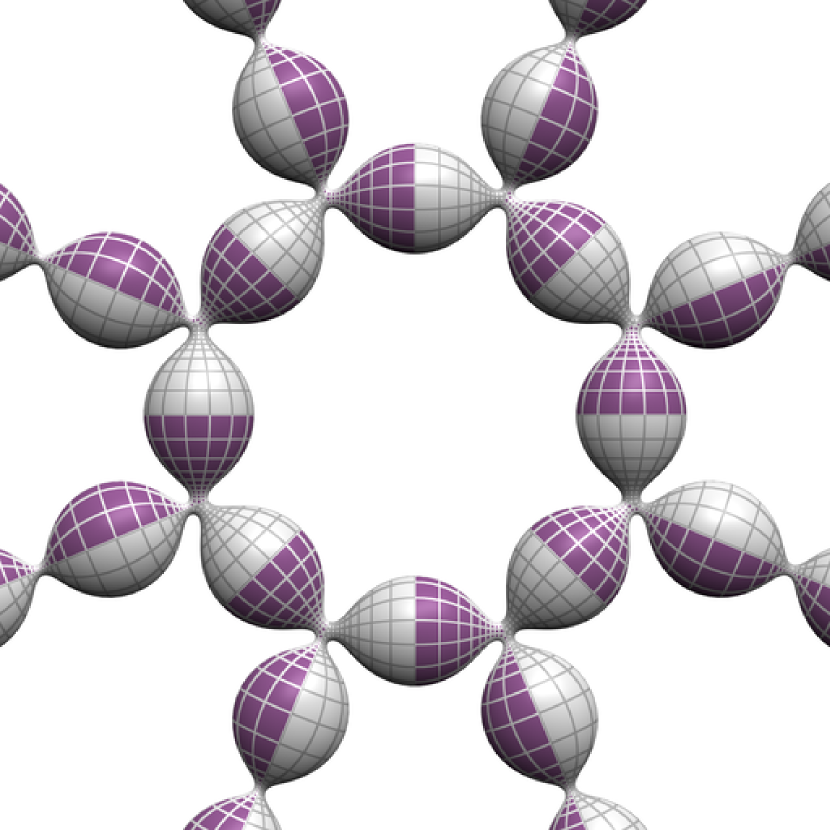
(c) torus 8 (neck)

Figure 21. CMC tori in $\mathbb{R}^{3}$ with Delaunay ends

Theorem 2.3.

Let $\xi$ be a meromorphic DPW potential satisfying the conditions of lemma 2.2 with $n$ singularities on $\mathbb{R}\cup\{\infty\}$ as above. Assume $\xi$ admits the reflection symmetry $\tau^{\ast}\xi(\lambda)=\overline{\xi(\overline{\lambda})}$ for $\tau(z)=\overline{z}$. Let $\theta_{ij}\in[0,\,\pi]$, $i,\,j\in\{1,\dots,n\}$, $i<j$. If the monodromies $M_{ij}$ satisfy

(2.13) $$\tfrac{1}{2}\operatorname{tr}M_{ij}|_{\lambda_{0}}=\text{--}(\operatorname*{spin}_{\gamma_{ij}}\xi)\cos\theta_{ij}\,\,\,,\quad i,\,j\in\{1,\dots,n\}\,\,\,,\quad i<j$$

then the CMC surface induced by $\xi$ with the upper halfplane as domain is a $n$-gon whose boundaries reflect in $n$ planes (respectively totally geodesic spheres) $P_{1},\dots,P_{n}$, with internal dihedral angles $\theta_{ij}$ between $P_{i}$ and $P_{j}$.

Proof.

Let $F$ be the unitary frame, $G$ a coordinate frame, with respect to a basis $\hat{e}_{0}$, $\hat{e}_{1}$, $\hat{e}_{2}\in\mathfrak{sl}({2},\,{\mathbb{C}})$ and $u$ the unitary $\lambda$-independent gauge between them, so $F=Gu$. By the proof of theorem 2.1(2), $\tau_{k}^{\ast}F=P_{k}\overline{F}$, $k\in\{1,\dots,n\}$ so

(2.14) $$\tau_{k}^{\ast}G=P_{k}\overline{G}Q_{k}^{\text{--}1}\,\,\,,\quad\tau^{\ast}u=Q_{k}\overline{u}\,\,\,.$$

Then with $\rho_{ij}$ and $\sigma_{ij}=\operatorname*{spin}_{\gamma_{ij}}u$,

(2.15a) $$u =\tau_{k}^{\ast}\tau_{k}^{\ast}u=Q_{k}\overline{Q}_{k}u\quad\implies\quad Q_{k}\overline{Q}_{k}=\operatorname{\mathbbm{1}}$$

(2.15b) $$\sigma_{ij}u =\rho^{\ast}u=\tau_{j}\tau_{i}u=Q_{j}Q_{i}^{\text{--}1}u\quad\implies\quad Q_{j}=\sigma_{ij}Q_{i}\,\,\,.$$

With $p_{k}$ a fixed point of $\tau_{k}$, define $u_{k}=u(p_{k})$ so $u_{k}=Q_{k}\overline{u}_{k}$. Then for $i,\,j\in\{1,\dots,n\}$, $i\neq j$, $u_{j}=Q_{j}\overline{u_{j}}=\sigma_{ij}Q_{i}\overline{u_{j}}$. Thus $u_{i}^{\text{--}1}u_{j}=\sigma_{ij}\overline{u_{i}^{\text{--}1}u_{j}}$. so

(2.16a) $$\sigma_{ij}=1 :\quad u_{i}^{\text{--}1}u_{j}=\overline{u_{i}^{\text{--}1}u_{j}}\quad\implies u_{i}^{\text{--}1}u_{j}e_{1}=e_{1}u_{i}^{\text{--}1}u_{j}$$

(2.16b) $$\sigma_{ij}=\text{--}1 :\quad u_{i}^{\text{--}1}u_{j}=-\overline{u_{i}^{\text{--}1}u_{j}}\quad\implies u_{i}^{\text{--}1}u_{j}e_{1}=-e_{1}u_{i}^{\text{--}1}u_{j}\,\,\,.$$

Hence $u_{i}^{\text{--}1}u_{j}=\sigma_{ij}e_{1}u_{i}^{\text{--}1}u_{j}$ so $u_{j}e_{1}u_{j}^{\text{--}1}=\sigma_{ij}u_{i}e_{1}u_{i}^{\text{--}1}$.

Let $e_{1}=\bigl{[}\begin{smallmatrix}0&1\\ \text{--}1&0\end{smallmatrix}\bigr{]}$. Since $G$ is a coordinate frame, we have ${(f_{y})}_{k}=G_{k}\hat{e}_{2}G_{k}^{\text{--}1}$. Define $\sigma_{k}\in\{\pm 1\}$ by $P_{k}e_{1}=\sigma_{k}{(f_{y})}_{k}$. Then

(2.17) $$N_{k}\mathrel{\vbox{\hbox{\scriptsize.}\hbox{\scriptsize.}}}=P_{k}e_{1}=F_{k}\overline{F}_{k}^{\text{--}1}e_{1}=F_{k}e_{1}F_{k}^{\text{--}1}=G_{k}u_{k}e_{1}u_{k}^{\text{--}1}G_{k}^{\text{--}1}=\sigma_{k}G_{k}\hat{e}_{2}G_{k}^{\text{--}1}$$

so

(2.18) $$u_{k}e_{1}u_{k}^{\text{--}1}=\sigma_{k}\hat{e}_{2}\,\,\,.$$

Hence $\sigma_{i}\sigma_{j}=\sigma_{ij}$.

Since $\tfrac{\mathrm{d}}{\mathrm{d}y}$ is pointing into the upper half plane, ${(f_{y})}_{k}$ is an internal normal to the plane. Thus $\sigma_{k}=1$ if $N_{k}$ is internal, and $\sigma_{k}=\text{--}1$ if $N_{k}$ is external. Thus $\sigma_{ij}=\sigma_{i}\sigma_{j}=1$ if and only if $N_{i}$ and $N_{j}$ are both internal or both internal, and $\sigma_{ij}=\sigma_{i}\sigma_{j}=\text{--}1$ if and only if one of $N_{i}$ and $N_{j}$ is internal and one external.

This means

(2.19) $$\langle N_{i},\,N_{j}\rangle=-\sigma_{ij}\cos\theta_{ij}$$

where $\theta_{ij}$ is the internal angle between planes $i$ and $j$. Since $M_{ij}=P_{j}P_{i}^{\text{--}1}$, then

(2.20) $$\tfrac{1}{2}\operatorname{tr}M_{ij}|_{\lambda=\lambda_{0}}=\langle N_{i},\,N_{j}\rangle=-\sigma_{ij}\cos\theta_{ij}\,\,\,.\qed$$

Remark 2.4.

Planes with dihedral angle $\theta_{ij}=\pi$ are parallel. Constraining the planes to coincide (for example, for the CMC torus with ends in $\mathbb{R}^{3}$) requires that the extrinsic conditions of theorem 2.3 be augmented with the additional condition

(2.21) $$\tfrac{\mathrm{d}}{\mathrm{d}\lambda}M_{ij}|_{\lambda=\lambda_{0}}=0\,\,\,.$$

It remains to control the vertices of the CMC polygon constructed in theorem 2.3. For this we use a DPW potential with simple poles:

Theorem 2.5.

Let $\xi$ a DPW potential as in theorem 2.3, $z_{k}$ a simple pole of $\xi$ on $\mathbb{R}$, and $\nu$ the eigenvalue of $\operatorname*{res}_{z=z_{k}}\xi$.

1. If $\nu=1/(2n)$ or $\nu=\tfrac{1}{2}-1/(2n)$, $n\in\mathbb{N}_{\geq 2}$, and $\xi_{-1}$ has a simple pole at $z_{k}$, then the CMC surface constructed from $\xi$ with $2n$ reflections around the vertex is immersed at the vertex.

2. If $\nu=\nu_{\mathrm{Del}}/n$, $n\in\mathbb{N}_{\geq 2}$, where $\nu_{\mathrm{Del}}$ is a Delaunay eigenvalue (2.2), then the CMC surface constructed from $\xi$ with $2n$ reflections around the vertex is a once-wrapped Delaunay end.

16cm(14.5cm,7.5cm)

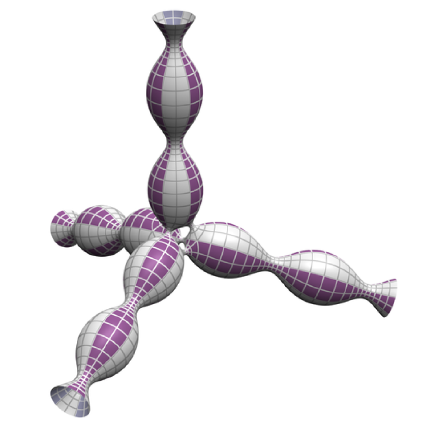
(a) tetrahedron (bulge)

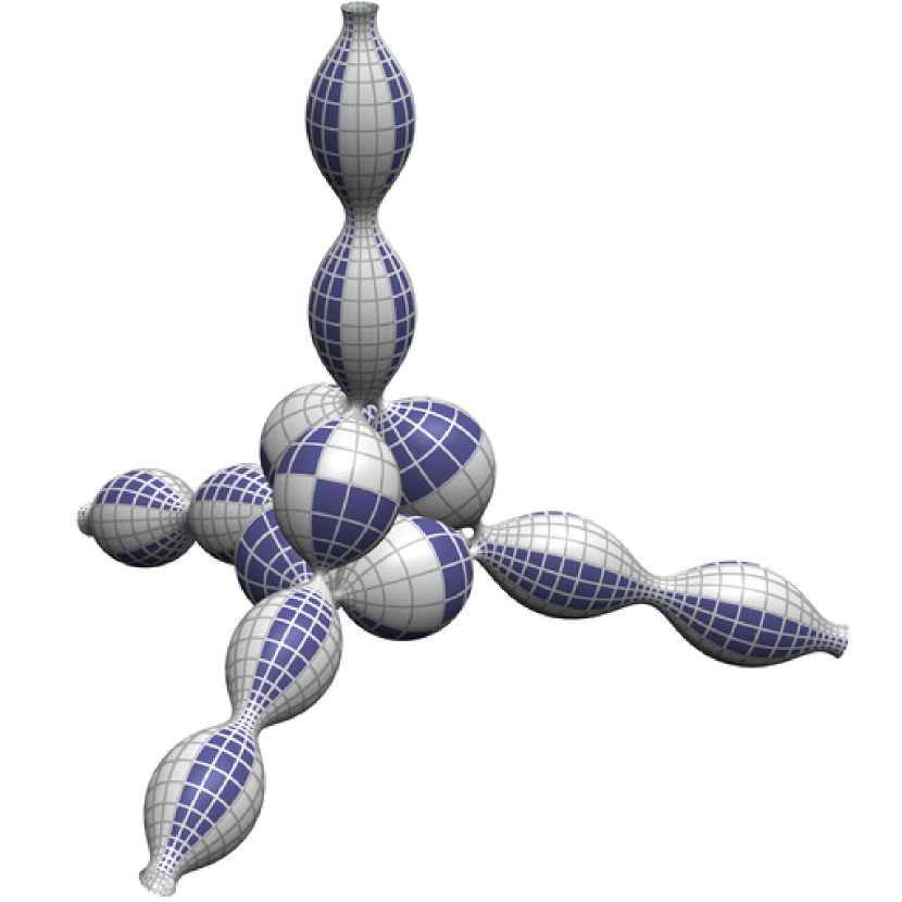
(b) tetrahedron (neck)

(c) octahedron

Figure 22. CMC surfaces in $\mathbb{R}^{3}$ with Platonic symmetry and Delaunay ends

Proof.

Assuming $z_{k}=0$, write $\xi=A_{\text{--}1}\mathrm{d}z/z+A_{0}\mathrm{d}z+\dots$. The pullback with respect to the local covering map $f(w)=w^{n}$ is

(2.22) $$f^{\ast}\xi=nA_{\text{--}1}\mathrm{d}w/w+nA_{0}w^{n-1}\mathrm{d}w+\dots\,\,\,.$$

Proof of (1): Since by assumption $A_{-1}$ has a pole at $\lambda=0$, by a $z$-independent local gauge of $\xi$ it may be assumed

(2.23) $$A_{\text{--}1}=\begin{bmatrix}1/(2n)&\lambda^{\text{--}1}\\ 0&\text{--}1/(2n)\end{bmatrix}\,\,\,.$$

Then the local gauge $g=\operatorname{diag}(w^{\text{--}1/2},\,w^{1/2})$ removes the simple pole of $f^{\ast}\xi$ at $w=0$, and

(2.24) $${{(f^{\ast}\xi)}{.}{g}}=\begin{bmatrix}0&n\lambda^{-1}\\ 0&1\end{bmatrix}\mathrm{d}w+\dots\,\,\,.$$

Since ${{(f^{\ast}\xi)}{.}{g}}$ is holomorphic at $w=0$ and its $\lambda^{-1}$ coefficient does not vanish at $w=0$, then the CMC surface induced by ${{(f^{\ast}\xi)}{.}{g}}$ is immersed at $w=0$. The proof for $\nu=\tfrac{1}{2}-1/(2n)$ is analogous.

Proof of (2): Since the eigenvalue of $A_{\text{--}1}$ is $\nu_{\mathrm{Del}}/n$, then the eigenvalue of $nA_{\text{--}1}$ is $\nu_{\mathrm{Del}}$, Unitary monodromy implies this is a once-wrapped Delaunay end. ∎

3. Symmetric CMC surfaces with genus

3.1. The potential

By applying a Möbius transformation we assume that the singular points of the CMC polygon are on the unit circle. As the fundamental piece is a CMC quadrilateral, we restrict to the 4-punctured sphere in the following. We will see in section 4 that, at least for surfaces without Delaunay ends, we can restrict without loss of generality to a Fuchsian DPW potential of the 4-punctured sphere. The means it has four simple poles and no pole at $z=\infty$, and is of the form

(3.1) $$\xi=\sum_{k=0}^{3}\frac{A_{k}}{z-z_{k}}\mathrm{d}z$$

as follows:

• The poles are $z_{0}\in\mathbb{S}^{1}$ in the open first quadrant, and $(z_{1},\,z_{2},\,z_{3})$ is a permutation of $(1/z_{0},\,-z_{0},\,-1/z_{0})$.

• The residues are

  (3.2a) $$A_{0}=\begin{bmatrix}y&\lambda^{-1}p\\ \frac{\lambda(\nu_{0}^{2}-y^{2})}{p}&-y\end{bmatrix}\,\,\,,\quad A_{2}=\begin{bmatrix}-y&\frac{(\nu_{1}^{2}-y^{2})}{x}\\ x&y\end{bmatrix}\,\,\,,\$$

  (3.2b) $$A_{1}=\sigma A_{0}\sigma^{-1}\,\,\,,\quad A_{3}=\sigma A_{2}\sigma^{-1}\,\,\,,\quad\sigma=\operatorname{diag}(\mathbbm{i},\,-\mathbbm{i})\,\,\,.$$

• For surfaces without Delaunay ends, the eigenvalue $\nu_{0}$ of $A_{0}$ and $A_{1}$ and $\nu_{1}$ of $A_{2}$ and $A_{3}$ are constants in $(0,\,1/2)$. For surfaces with Delaunay ends, $\nu_{0}$ is of the form $c\nu_{\mathrm{Del}}$ with $c\in(0,\,1)$ and $\nu_{\mathrm{Del}}$ is the eigenvalue of a Delaunay unduloid

  (3.3) $$\nu_{\mathrm{Del}}=\tfrac{1}{2}\sqrt{1+\tfrac{1}{4}\lambda^{\text{--}1}{(\lambda-1)}^{2}w}\,\,\,,\quad w\in(0,\,1]\,\,\,.$$

• The accessory parameters $x$ and $y$ are holomorphic functions of $\lambda$ on an open disk $\mathcal{D}_{r}$ of radius $r>0$ centered at the origin satisfying $x(\overline{\lambda})=\overline{x(\lambda)}$ and $y(\overline{\lambda})=\overline{y(\lambda)}$. The function $p$ is a monic polynomial in $\lambda$ satisfying $p(\overline{\lambda})=\overline{p(\lambda)}$.

• The quotients $\lambda(\nu_{0}^{2}-y^{2})/p$ and $(\nu_{1}^{2}-y^{2})/x$ are holomorphic functions of $\lambda$ on $\mathcal{D}_{r}$.

The need for the last condition is as follows. The unitary flow, which preserves the unitarizability of the monodromy of $\xi$, is implemented by evaluating the monodromy of $\xi$ directly on the unit circle, and not by the numerically more problematic procedure of computing the monodromy on an $r<1$ circle and then extending it to the unit circle.

Let $M_{k}$ ($k\in\{0,\dots,3\}$) be the local monodromy around $z_{k}$ based at $z=1$.

The surfaces are constructed by running the unitary flow (see section 3.3 below) so that at the end of the flow for $k=0,1$

(3.4a) $$\nu_{0}|_{\lambda=\lambda_{k}}=\tfrac{1}{2n_{0}}\,\,\,,\quad\nu_{1}|_{\lambda=\lambda_{k}}=\tfrac{1}{2}-\tfrac{1}{2n_{1}}\,\,\,,\quad$$

(3.4b) $$\operatorname{tr}M_{0}M_{1}|_{\lambda=\lambda_{k}}=-\cos\tfrac{2\pi}{r}\,\,\,,\quad\tfrac{1}{2}\operatorname{tr}M_{1}M_{2}|_{\lambda=\lambda_{k}}=\cos\tfrac{\pi}{s}\,.$$

Then, by theorems 2.3 and 2.5, the unit $z$-disk maps to a CMC quadrilateral whose edges reflect in planes (respectively geodesic 2-spheres) with internal dihedral angles specified by the figure at right, and whose vertices after these reflections are either immersed points or once-wrapped Delaunay ends.

In the special case $\nu_{0}+\nu_{1}=\tfrac{1}{2}$, the surfaces are constructed by running the unitary flow so that at the end of the flow for $k=0,1$

(3.5a) $$\nu_{0}|_{\lambda=\lambda_{k}}=\tfrac{1}{2n_{0}}\,\,\,,\quad\nu_{1}|_{\lambda=\lambda_{k}}=\tfrac{1}{2}-\tfrac{1}{2n_{0}}\,\,\,,\quad$$

(3.5b) $$\operatorname{tr}M_{0}M_{1}|_{\lambda=\lambda_{k}}=-\cos\tfrac{2\pi}{r}\,\,\,,\quad\tfrac{1}{2}\operatorname{tr}M_{1}M_{2}|_{\lambda=\lambda_{k}}=\cos\tfrac{2\pi}{s}$$

Then the quarter disk in the first quadrant maps to a CMC quadrilateral whose edges reflect in planes with internal dihedral angles specified by the figure at right, and whose vertices after these reflections are immersed.

3.2. The initial condition

3.2.1. The initial condition

The initial condition for the unitary flow is a potential $\xi_{0}$ of the form in section 3.1 with eigenvalues $\nu_{0}=\nu_{1}=\tfrac{1}{4}$ with unitary monodromy on $\mathbb{S}^{1}$ which induces a Delaunay surface.

16cm(14.5cm,7.5cm)

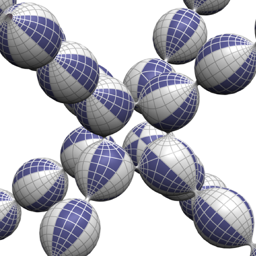
(a) cube

(b) icosahedron

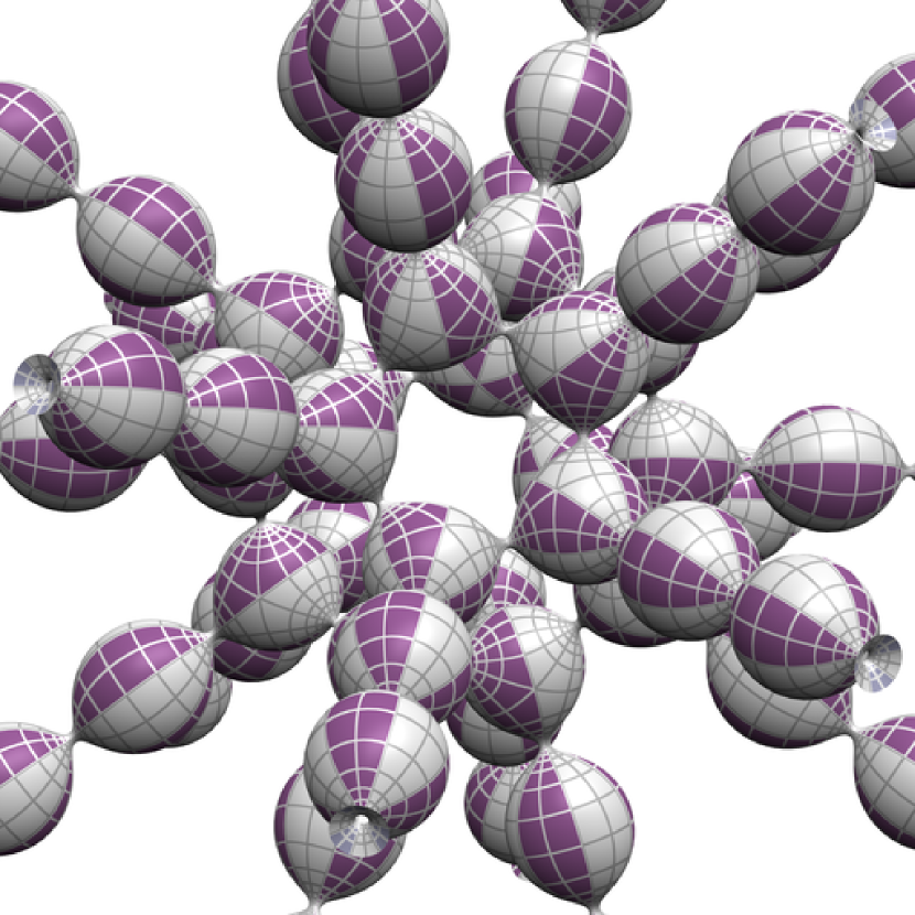
(c) dodecahedron

Figure 23. CMC surfaces in $\mathbb{R}^{3}$ with Platonic symmetry and Delaunay ends

Lemma 3.1.

1. For CMC tori of spectral genus $0$ the spectral curve $\pi:\mathbb{C}\mathrm{P}^{1}\to\mathbb{C}\mathrm{P}^{1}$ can be chosen to be $\pi(\xi)=\xi^{2}$. The involutions are

   (3.6) $$\sigma(\xi)=-\xi\,\,\,,\quad\rho(\xi)=\overline{\xi}^{-1}\,\,\,,\quad\kappa(\xi)=\overline{\xi}\,\,\,.$$

   The monodromy eigenvalues of the vacuum are $\exp(\pm\nu_{1}+2\mathbbm{i}\pi\mathbb{Z})$, $\exp(\pm\nu_{2}+2\mathbbm{i}\pi\mathbb{Z})$ where

   (3.7) $$\nu_{1}(\xi)\mathrel{\vbox{\hbox{\scriptsize.}\hbox{\scriptsize.}}}=\mathbbm{i}\pi\frac{\xi-\xi^{-1}}{\xi_{0}-\xi_{0}^{-1}}\,\,\,,\quad\nu_{2}(\xi)\mathrel{\vbox{\hbox{\scriptsize.}\hbox{\scriptsize.}}}=\mathbbm{i}\pi\frac{\xi+\xi^{-1}}{\xi_{0}+\xi_{0}^{-1}}$$

   and $\pi(\pm\xi_{0}),\,\pi(\pm\xi_{0}^{-1})\in\mathbb{S}^{1}$ are the evaluation points.

2. For some $\ell,\,m\in\mathbb{Z}^{+}$ the monodromy eigenvalues of a Delaunay cylinder are $\exp(\pm\nu_{1}+2\mathbbm{i}\pi\mathbb{Z})$, $\exp(\pm\nu_{2}+2\mathbbm{i}\pi\mathbb{Z})$ where

   (3.8a) $$\nu_{1}(u)\mathrel{\vbox{\hbox{\scriptsize.}\hbox{\scriptsize.}}}=\mathbbm{i}\pi\frac{f_{1}(u)-f_{2}(u)}{f_{1}(u_{0})-f_{2}(u_{0})}\,\,\,,$$

   (3.8b) $$\nu_{2}(u)=\tfrac{1}{2}\ell(f_{1}(u)+f_{2}(u))\,\,\,,\quad\nu_{2}(u_{0})=\mathbbm{i}\pi m\,\,\,,$$

   where $\pi(\pm u_{0})$, $\pi(\pm\overline{u_{0}}+\tfrac{1}{2}\omega_{1})\in\mathbb{S}^{1}$ are the evaluation points, and $f_{1},\,f_{2}$ are as in (3.9).

On the torus $\mathbb{C}/(\mathbb{Z}+\tau\mathbb{Z})$, Let $\wp$ be the Weierstrass function and let $\zeta\mathrel{\vbox{\hbox{\scriptsize.}\hbox{\scriptsize.}}}=-\int\wp$. Let $\{\omega_{1},\,\omega_{2},\,\omega_{3}\}=\{\tfrac{1}{2},\,\tfrac{1}{2}+\tfrac{\tau}{2},\,\tfrac{\tau}{2}\}$.

Define on some torus with modulus $\tau_{\mathrm{spec}}$

(3.9) $$h_{1}(u)\mathrel{\vbox{\hbox{\scriptsize.}\hbox{\scriptsize.}}}=\eta_{1}u-\omega_{1}\zeta(u)\,\,\,,\quad h_{2}(u)\mathrel{\vbox{\hbox{\scriptsize.}\hbox{\scriptsize.}}}=f_{1}(u-\tfrac{1}{2}\omega_{1})\,\,\,.$$

The theta function

(3.10) $$\theta(x,\,\tau)\mathrel{\vbox{\hbox{\scriptsize.}\hbox{\scriptsize.}}}=\sum_{k\in\mathbb{Z}}\exp\bigl{(}2\mathbbm{i}\pi(\tfrac{1}{2}n^{2}\tau+n(x-\omega_{2})\bigr{)}$$

is an entire function $\mathbb{C}\to\mathbb{C}$ with simple zeros at lattice points $\mathbb{Z}+\tau\mathbb{Z}$ and no other zeros, satisfying

(3.11) $$\theta(x+1)=\theta(x)\,\,\,,\quad\theta(x+\tau)=-\exp(-2\mathbbm{i}\pi x)\theta(x)\,\,\,,\quad\theta(\tau-x)=\theta(x)$$

for all $x\in\mathbb{C}$. Define

(3.12a) $$\tfrac{1}{2}g_{0}(\tfrac{1}{2}x) =\frac{\theta^{\prime}(x)}{\theta(x)}-\frac{2\theta^{\prime}(\tfrac{1}{2}x)}{\theta(\tfrac{1}{2}x)}+\mathbbm{i}\pi\,\,\,,$$

(3.12b) $$\tfrac{1}{2}g_{k}(\tfrac{1}{2}x) =\exp\bigl{(}2\mathbbm{i}\pi x\tfrac{\omega_{k}-\overline{\omega_{k}}}{\tau-\overline{\tau}}\bigr{)}\frac{\theta(x+\omega_{k})\theta^{\prime}(0)}{\theta(x)\theta(\omega_{k})}\,\,\,,\quad k\in\{1,\,2,\,3\}\,\,\,.$$

16cm(14.5cm,1cm)

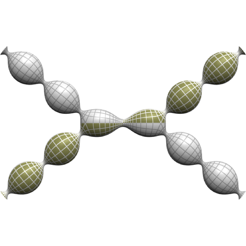
(a) fournoid

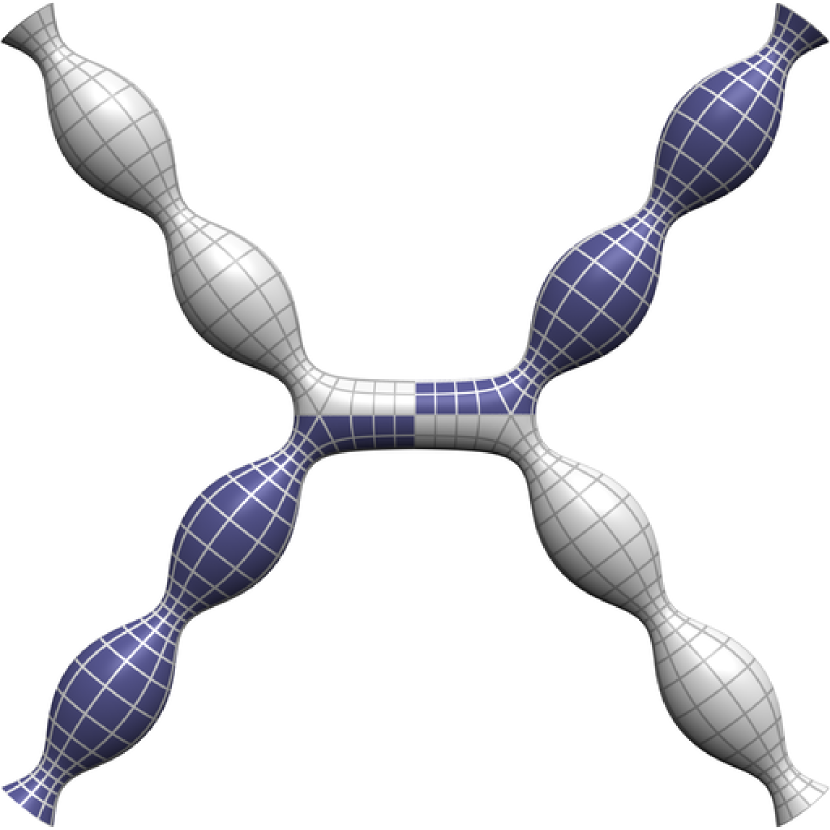
(b) fournoid

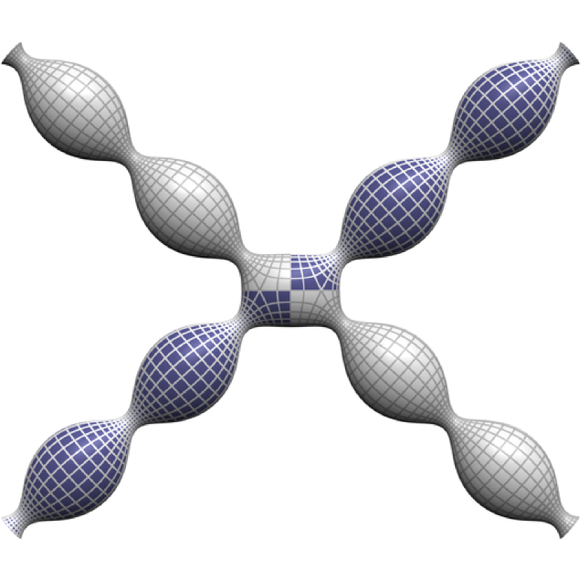
(c) fournoid

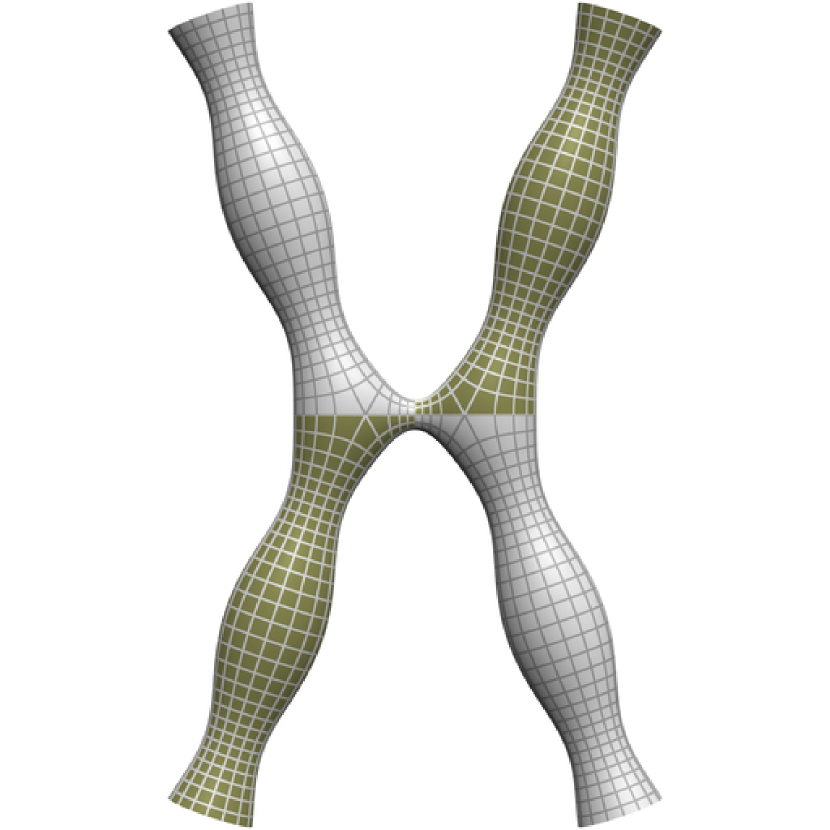
(d) fournoid

Figure 24. CMC sphere in $\mathbb{R}^{3}$ with Delaunay ends

The initial condition is the potential in section 3.1 with

(3.13a) $$x=\lambda(y+\nu_{0})(y+\nu_{1})\frac{1-u}{1+u}\,\,\,,\quad y(b,\,a)=-\frac{\tfrac{2\mathbbm{i}\pi}{\tau-\overline{\tau}}(b+a)+f_{0}(b)}{2g_{2}(\tfrac{1}{2}b)}$$

(3.13b) $$u(b)=-\frac{g_{1}(\tfrac{1}{2}b)}{g_{3}(\tfrac{1}{2}b)}\,\,\,,\quad v(b,\,a)=\frac{\tfrac{2\mathbbm{i}\pi}{\tau-\overline{\tau}}(b+a)+f_{0}(b)}{g_{2}(\tfrac{1}{2}b)}$$

(3.13c) $$a=\tfrac{2\mathbbm{i}\pi}{\tau-\overline{\tau}}\tfrac{1}{2}h_{1}\,\,\,,\quad b=\tfrac{2\mathbbm{i}\pi}{\tau-\overline{\tau}}\tfrac{1}{2}h_{2}$$

(3.13d) $$\nu_{0}=\nu_{1}=\tfrac{1}{4}\,\,\,,\quad[z_{0},\,z_{1},\,z_{2},\,z_{3}]=u(\omega_{2})^{2}\,\,\,,\quad p=1\,\,\,.$$

The initial condition is computed numerically from (3.13a) as Laurent series on $\mathbb{S}^{1}$ by computing its Fourier coefficients. The initial data can be computed from Lemma (3.1) using results from [11]

3.2.2. Configurations of the initial condition

Permuting the lattice generators in the initial condition creates different arrangements of residues of the DPW potential on the Delaunay cylinder. For the configurations used in this report, the two circle arcs ($z_{0},\,z_{1})$ and $(z_{2},\,z_{3})$ are mapped to semicircles (resp. profile curves) on the Delaunay surface, while the other two circle arcs ($z_{1},\,z_{2})$ and $(z_{3},\,z_{0})$ are mapped to profile curves (resp. semicircles) on the Delaunay surface. The first of these configurations is used to compute the 2-dimensional lattices and the cubic lattices; the second is used to compute the tori and Platonic surfaces with ends.

3.2.3. Neck and bulge

For the initial potential $\xi_{0}$ above, the poles of the Fuchsian DPW potential are at necks of the Delaunay surface. The initial potential with poles at bulges is constructed as a gauge of $\xi_{0}$ by the gauge $\operatorname{diag}({(\lambda-\lambda_{0})}^{-1/2},{(\lambda-\lambda_{0})}^{1/2})$, where the $\lambda_{0}$ is a common zero of $x$ and $y^{2}-1/16$. This gauge is not a DPW gauge, but a so-called dressing transformation.

3.3. The unitary flow

3.3.1. The unitary flow

The unitary flow is a flow through the space of potentials of section 3.1 preserving the intrinsic closing condition. It starts at a potential in the space with unitary monodromy, and flows until the monodromy at the evaluation points reach some desired extrinsic closing conditions.

Given a smooth function $F=F(t,\,\vec{x}):\mathbb{R}^{1+n}\to\mathbb{R}^{n}$ encoding $n$ conditions on a flow parameter $t\in[0,\,1]$ and $n$ variables $\vec{x}$, if $\det\frac{\mathrm{d}F}{\mathrm{d}x}\neq 0$, then $x(t)$ satisfying $F(t,\,x(t))=0$ can be computed by the implicit ODE $\frac{\mathrm{d}F}{\mathrm{d}t}+\frac{\mathrm{d}F}{\mathrm{d}x}\frac{\mathrm{d}x}{\mathrm{d}t}=0.$ The solution for the infinite case can be computed numerically by truncating to $F:\mathbb{R}^{1+n}\to\mathbb{R}^{m}$, $m\geq n$, and solving the resulting finite dimensional ODE by least squares methods.

The variables $\vec{x}$ parametrizing the potential consists of:

• the conformal type $[z_{0},\,z_{1},\,z_{2},\,z_{3}]$

• the local eigenvalues $\nu_{0}|_{\lambda=1}$ and $\nu_{1}|_{\lambda=1}$

• the end weight $w_{0}$

• the polynomial $p$

• the accessory parameters $x$ and $y$.

The accessory parameters, which are holomorphic functions of $\lambda$, are approximated by truncating their power series at $\lambda=0$. We always assume that these functions extend to a disc $D_{r}$ with $r>1$ so that the first bullet point below can be checked directly on the unit circle.

The constraints $F=0$ are of two types:

• the intrinsic closing conditions: the halftraces $t_{ij}=\tfrac{1}{2}\operatorname{tr}M_{i}M_{j}$, $i,\,j\in\{0,\dots,3\}$, $i<j$ are real on $\mathbb{S}^{1}$. This is a necessary condition by theorem 3.4.

• geometric constraints which choose a path through the space of geometric parameters to reach the desired extrinsic closing conditions at the end of the flow.

By theorem 3.4 the monodromy is unitarizable if all halftraces along the unit circle are real and of absolute value less or equal to 1. As the components of irreducible $\mathrm{SL}(2,\mathbb{C})$-representations of the 4-punctured sphere with real traces consists entirely of either $\mathrm{SL}(2,\mathbb{R})$ or $\mathrm{SU}(2)$ representations, and since $\xi_{0}$ is unitarizable, we can ignore the condition that all traces are of absolute value less or equal to 1 during the unitary flow.

16cm(14.5cm,7.5cm)

(a) Lawson $\xi_{12}$

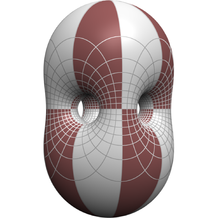
(b) Lawson $\xi_{13}$

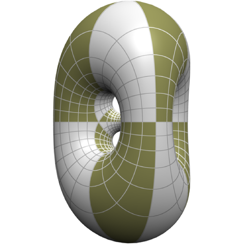
(c) Lawson $\xi_{22}$

Figure 25. Minimal Lawson surfaces in $\mathbb{S}^{3}$

The intrinsic closing conditions on $\mathbb{S}^{1}_{\lambda}$ are approximated by evaluation at finitely many equally spaced sample points on $\mathbb{S}^{1}_{\lambda}$. In the following we describe the other constraints in more detail:

3.3.2. Geometric constraints

The simplest configuration of the geometric constraints are as follows. The two local and two global eigenvalues depend linearly on the flow parameter $t$ to reach the desired values at $t=1$. If the surface has no ends, the end weight $w_{0}$ is set to $0$; otherwise it depends linearly on $t$ starting at $0$ and reaching a heuristically chosen value at $t=1$. In this configuration the conformal type is fixed during the flow.

It is possible that the flow with this simple configuration breaks down, in which case the path must be modified in some heuristically determined way, for example by making the conformal type depend on the flow parameter.

In practice each geometric parameter is of one of three types:

• fixed during the flow

• depending linearly on the flow parameter $t$

• free (unconstrained).

Then the fixed variables, and the variables depending on $t$, being computable from $t$, can be omitted from $\vec{x}$.

3.4. Irreducibility and unitarizability

For a subgroup $\mathcal{G}\subset{\mathrm{SL}}_{2}{\mathbb{C}}$ generated by three elements, this section proves

• a necessary and sufficient condition for the irreducibility of $\mathcal{G}$, and

• a necessary condition for the ${\mathrm{SU}}_{2}{}$ unitarizability of $\mathcal{G}$, assuming $\mathcal{G}$ is irreducible.

Here, a group $\mathcal{G}$ is reducible if all elements have a common eigenline, and is ${\mathrm{SU}}_{2}{}$ unitarizable if there exists $C\in{\mathrm{SL}}_{2}{\mathbb{C}}$ such that $C\mathcal{G}C^{\text{--}1}\subset{\mathrm{SU}}_{2}{}$. The methods used in the proofs can be generalized to any finitely generated group.

The proof depends on the following lemma 3.2, which determines to what extend three elements of $\mathbb{C}^{3}$ are determined by their standard $\mathbb{C}^{3}$ inner products.

With $\langle-,\,-\rangle$ the standard inner product on $\mathbb{C}^{3}$, let $\mathcal{L}=\{v\in\mathbb{C}^{3}\operatorname{|}\langle v,\,v\rangle=0\}$. Let $X=(x_{0},\,x_{1},\,x_{2})\in{\mathrm{M}}_{3\times 3}{\mathbb{C}}$, with columns $x_{0},\,x_{1},\,x_{2}\in\mathbb{C}^{3}$. Let $W={{X}^{\top}}X\in{\mathrm{Sym}}_{n}{\mathbb{C}}$, so $W_{ij}=\langle x_{i},\,x_{j}\rangle$.

Lemma 3.2.

With $X$ and $W$ as above,

1. $\ker{{X}^{\top}}\cap\mathcal{L}=\{0\}$ if and only if $\operatorname{rank}W\geq 2$.

2. Assuming (a), if for some $Y\in{\mathrm{M}}_{3\times 3}{\mathbb{C}}$, ${{X}^{\top}}X={{Y}^{\top}}Y$ and $\det X=\det Y$, then there exists a unique $S\in{\mathrm{SO}}_{3}{\mathbb{C}}$ such that $Y=SX$.

Proof.

By the rank-nullity theorem applied to ${{X}^{\top}}|_{\operatorname{image}X}$,

(3.14) $$\operatorname{rank}X=\dim(\ker{{X}^{\top}}\cap\operatorname{image}X)+\operatorname{rank}W$$

from which it follows that $\operatorname{rank}X\geq\operatorname{rank}W$, and $\operatorname{rank}W=3$ if $\operatorname{rank}X=3$.

Moreover, if $\operatorname{rank}X\geq 2$, then

(3.15) $$\ker{{X}^{\top}}\cap\operatorname{image}X=\ker{{X}^{\top}}\cap\mathcal{L}\,\,\,.$$

To prove (1), assume $\operatorname{rank}W\geq 2$, so $\operatorname{rank}X=2$. By (3.14), $\dim(\ker{{X}^{\top}}\cap\operatorname{image}X)=0$. By (3.15), $\ker{{X}^{\top}}\cap\mathcal{L}=\{0\}$.

Conversely, assume $\ker{{X}^{\top}}\cap\mathcal{L}=\{0\}$. Then $\operatorname{rank}X\geq 2$ because every $2$-dimensional subspace of $\mathbb{C}^{3}$ intersects $\mathcal{L}$. By (3.15), $\ker{{X}^{\top}}\cap\mathcal{L}=\{0\}$. By (3.14), $\operatorname{rank}W=\operatorname{rank}X\geq 2$.

To prove (2) in the case $\operatorname{rank}W=3$, since $\operatorname{rank}X=\operatorname{rank}Y=3$, define $S\mathrel{\vbox{\hbox{\scriptsize.}\hbox{\scriptsize.}}}=YX^{-1}$. Then $S\in{\mathrm{SO}}_{3}{\mathbb{C}}$ by ${{X}^{\top}}X={{Y}^{\top}}{Y}$ and $\det X=\det Y$.

To prove (2) in the case $\operatorname{rank}W=2$, let $x_{a},\,x_{b}$ be two independent columns of $X$ and let $\hat{X}=(x_{a},\,x_{b},\,x_{a}\times x_{b})$ and $\hat{Y}=(y_{a},\,y_{b},\,y_{a}\times y_{b})$. Since $x_{a}\times x_{b}\in\ker{{X}^{\top}}$, then by the assumption and lemma 3.2(1), $x_{a}\times x_{b}\not\in\mathcal{L}$. Then $\det\hat{X}=\langle x_{a}\times x_{b},\,x_{a}\times x_{b}\rangle\neq 0$ so $\operatorname{rank}\hat{X}=3$. Moreover, since $\langle x_{a}\times x_{b},\,x_{a}\times x_{b}\rangle=\langle y_{a}\times y_{b},\,y_{a}\times y_{b}\rangle$, then ${{\hat{X}}^{\top}}\hat{X}={{\hat{Y}}^{\top}}\hat{Y}$. Then $S\mathrel{\vbox{\hbox{\scriptsize.}\hbox{\scriptsize.}}}=\hat{Y}\hat{X}^{-1}$ is in ${\mathrm{SO}}_{3}{\mathbb{C}}$, and $Y=SX$. ∎

16cm(14.5cm,7.5cm)

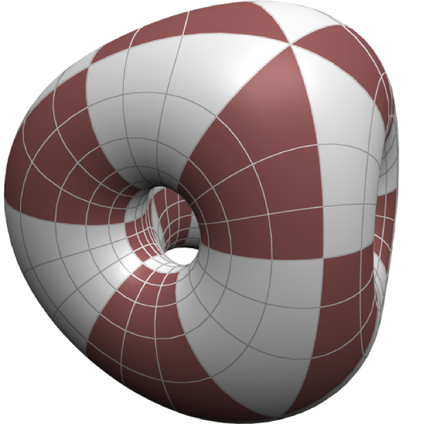
(a) tetrahedron

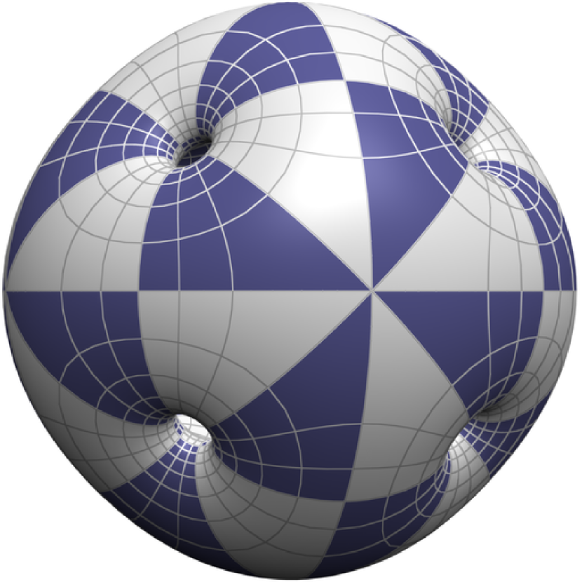
(b) octahedron

(c) cube

Figure 26. Minimal surfaces in $\mathbb{S}^{3}$ with Platonic symmetry

Identify $\mathbb{C}^{4}$ with $\mathfrak{gl}({2},\,{\mathbb{C}})$ by identifying the standard basis $E_{0},\,E_{1},\,E_{2},\,E_{3}$ with $\operatorname{\mathbbm{1}},\,e_{0},\,e_{1},\,e_{2}$, where

(3.16) $$e_{0}\mathrel{\vbox{\hbox{\scriptsize.}\hbox{\scriptsize.}}}=\bigl{[}\begin{smallmatrix}\mathbbm{i}&0\\ 0&\text{--}\mathbbm{i}\end{smallmatrix}\bigr{]}\,\,\,,\quad e_{1}\mathrel{\vbox{\hbox{\scriptsize.}\hbox{\scriptsize.}}}=\bigl{[}\begin{smallmatrix}0&1\\ -1&0\end{smallmatrix}\bigr{]}\,\,\,,\quad e_{2}\mathrel{\vbox{\hbox{\scriptsize.}\hbox{\scriptsize.}}}=\bigl{[}\begin{smallmatrix}0&\mathbbm{i}\\ \text{--}\mathbbm{i}&0\end{smallmatrix}\bigr{]}\,\,\,.$$

Under this identification, the standard inner product on $\mathbb{C}^{4}$ is

(3.17) $$\langle x,\,y\rangle=\tfrac{1}{2}\operatorname{tr}x\operatorname{adj}(y)\,\,\,,\quad\operatorname{adj}\bigl{[}\begin{smallmatrix}a&b\\ c&d\end{smallmatrix}\bigr{]}\mathrel{\vbox{\hbox{\scriptsize.}\hbox{\scriptsize.}}}=\bigl{[}\begin{smallmatrix}d&-b\\ -c&a\end{smallmatrix}\bigr{]}$$

and ${\mathrm{SU}}_{2}{}\subset{\mathrm{SL}}_{2}{\mathbb{C}}$ is identified with $\mathbb{R}^{4}\subset\mathbb{C}^{4}$. In particular, for $X,\,Y\in\mathfrak{sl}({2},\,{\mathbb{C}})$ it holds $\langle x,\,y\rangle=-\tfrac{1}{2}\operatorname{tr}xy$.

In order to treat irreducibility, the following lemma translates the notion of eigenline to a more convenient form. With $\bigl{[}\begin{smallmatrix}a\\ b\end{smallmatrix}\bigr{]}^{\perp}\mathrel{\vbox{\hbox{\scriptsize.}\hbox{\scriptsize.}}}=[\begin{smallmatrix}-b&a\end{smallmatrix}]$ consider the double cover

(3.18) $$\hat{x}\in\mathbb{C}^{2}\setminus\{0\}\to\{x\in\mathfrak{sl}({2},\,{\mathbb{C}})\operatorname{|}\det x=0\}\,\,\,,\quad\hat{x}\mapsto x=\hat{x}\hat{x}^{\perp}\,\,\,.$$

Lemma 3.3.

$\ell\in\mathbb{C}^{2}\setminus\{0\}$ is an eigenvector of the invertible matrix $x\in{\mathrm{SL}}_{2}{\mathbb{C}}$ if and only if $\langle x,\,\ell\ell^{\perp}\rangle=0$.

Proof.

For any $p,\,q\in\mathbb{C}^{2}\setminus\{0\}$,

(3.19) $$\operatorname{tr}qp^{\perp}=p^{\perp}q=\det(p,\,q)\,\,\,.$$

So with $p=\ell$, $q=x\ell$, and $y=\ell\ell^{\perp}$

(3.20) $$2\langle x,\,y\rangle=2\langle x,\,\ell\ell^{\perp}\rangle=\det(x\ell,\,\ell)$$

so $\langle x,\,y\rangle=0$ if and only if $x\ell$ and $\ell$ are dependent, that is, if and only if $\ell$ is an eigenline of $x$. ∎

Let $\mathcal{P}$ be the group generated by $P_{0}=\operatorname{\mathbbm{1}},\,P_{1},\,P_{2},\,P_{3}\in{\mathrm{SL}}_{2}{\mathbb{C}}$. Under the above identification $\mathbb{C}^{4}\cong\mathfrak{gl}({2},\,{\mathbb{C}})$ let $P=(P_{0},\,P_{1},\,P_{2},\,P_{3})\in{\mathrm{M}}_{4\times 4}{\mathbb{C}}$ be a matrix with columns $P_{k}\in\mathbb{C}^{4}$. Let $T={{P}^{\top}}P\in{\mathrm{Sym}}_{4}{\mathbb{C}}$, so $T_{ij}=\langle P_{i},\,P_{j}\rangle$.

Theorem 3.4.

With $P$ and $T$ as above,

1. $\mathcal{P}$ is irreducible if and only if $\operatorname{rank}T\geq 3$.

2. Assuming (1), $\mathcal{P}$ is ${\mathrm{SU}}_{2}{}$ unitarizable if and only if $T$ is real positive semidefinite.

Proof.

We have the factorization

(3.21) $$T=\begin{bmatrix}\operatorname{\mathbbm{1}}&0\\ {{V}^{\top}}&\operatorname{\mathbbm{1}}\end{bmatrix}\begin{bmatrix}\operatorname{\mathbbm{1}}&0\\ 0&{{X}^{\top}}\end{bmatrix}\begin{bmatrix}\operatorname{\mathbbm{1}}&0\\ 0&X\end{bmatrix}\begin{bmatrix}\operatorname{\mathbbm{1}}&V\\ 0&\operatorname{\mathbbm{1}}\end{bmatrix}\,\,\,,\quad P=\begin{bmatrix}1&V\\ 0&X\end{bmatrix}\,\,\,.$$

To prove (1), let $X=(x_{0},\,x_{1},\,x_{2})\in{\mathrm{M}}_{3\times 3}{\mathbb{C}}$ be the lower right $3\times 3$ submatrix of $P$, that is the matrix with columns given by the tracefree parts of $P_{1},\,P_{2},\,P_{3}$, and let $Y\mathrel{\vbox{\hbox{\scriptsize.}\hbox{\scriptsize.}}}={{X}^{\top}}X$. By lemma 3.3, $\mathcal{P}$ is irreducible if and only if $\ker{{X}^{\top}}\cap\mathcal{L}=\{0\}$. By lemma 3.2 this is if and only if $\operatorname{rank}Y\geq 2$. Since $\operatorname{rank}T=1+\operatorname{rank}Y$, this is if and only if $\operatorname{rank}T\geq 3$.

To prove (2), if $\mathcal{P}$ is ${\mathrm{SU}}_{2}{}$ unitarizable, it may be assumed without loss of generality that $\mathcal{P}\subset{\mathrm{SU}}_{2}{}$. Then $P\in{\mathrm{M}}_{4\times 4}{\mathbb{R}}$, so $T={{T}^{\top}}T\in{\mathrm{Sym}}_{4}{\mathbb{R}}$ is real positive semidefinite.

Conversely, if $T$ is real positive semidefinite, then $W={{X}^{\top}}X={{Y}^{\top}}Y$ for some $Y\in{\mathrm{M}}_{3\times 3}{\mathbb{R}}$. Replacing $Y\mapsto\text{--}Y$ if necessary, then $\det X=\det Y$, so by lemma 3.2(2), there exists $S\in{\mathrm{SO}}_{3}{\mathbb{C}}$ such that $X=SY$. Let $C\in{\mathrm{SL}}_{2}{\mathbb{C}}$ be a lift of $S$ via the double cover ${\mathrm{SL}}_{2}{\mathbb{C}}\mapsto{\mathrm{SO}}_{3}{\mathbb{C}}$ defined with respect to $\operatorname{\mathbbm{1}},\,e_{1},\,e_{2},\,e_{3}$. Note that this double cover is given by conjugation on $\mathfrak{sl}({2},\,{\mathbb{C}})\cong\mathbb{C}^{3}$. Then $C$ unitarizes $\mathcal{P}$. ∎

3.5. Constructing the surface

Once the potential for a surface is obtained via the unitary flow, the surface is constructed as follows:

• Compute the unitarizer of the monodromy.

• Compute curvature lines.

• Compute the fundamental piece of the surface via the DPW construction

• Build the surface from the fundamental piece by reflections.

3.5.1. The unitarizer

Due to the symmetry (3.2) of the potential and of the monodromies with basepoint $z=1$ the unitarizer is diagonal and can be computed as follows. With the notation $a^{\ast}(\lambda)=\overline{a(1/\overline{\lambda})}$ write

(3.22) $$M_{0}=\begin{bmatrix}a&b\\ c&a^{\ast}\end{bmatrix}\,\,\,.$$

By the unitarizability of $M_{0}$ by a diagonal loop, $p\mathrel{\vbox{\hbox{\scriptsize.}\hbox{\scriptsize.}}}=-c^{\ast}/b=-c/b^{\ast}$ takes values in $\mathbb{R}_{+}$ along $\mathbb{S}^{1}$ away from its zeros and poles, which are even. Let $f=\prod(\lambda-\alpha)/\prod(\lambda-\beta)$ so that $f^{\ast}f$ has the same zeros and poles as $p$. Then $q=p/(f^{\ast}f)$ takes values in $\mathbb{R}_{+}$ along $\mathbb{S}^{1}$ without zeros or poles. Let $y^{\ast}y=q$ be the scalar ${\mathrm{GL}}_{1}{\mathbb{C}}$ Birkhoff factorization, so $y$ is holomorphic in the unit disk. Then with $x=fy$ the loop $\operatorname{diag}({x}^{1/2},\,{x}^{-1/2})$ is the required unitarizer, holomorphic on the open unit disk.

3.5.2. Curvature lines

Let $Q=q(z)\mathrm{d}z^{2}$ the Hopf differential of the CMC surface. The curvature line coordinate $v$ satisfies $\mathrm{d}v^{2}=Q(z)\mathrm{d}z^{2}$. Curvature line coordinates can be computed by computing $\int\!\!\sqrt{Q(z)}\,\mathrm{d}z$ over the domain.

The surface is computed numerically by dividing the domain into polygons (triangles or quadrilaterals) and mapping via the CMC immersion these triangles to $\mathbb{R}^{3}$. In the computation of curvature lines described above, the polygon edges are unrelated to the curvature lines.

Quadrilaterals whose edges are along curvature lines can be computed as follows. Divide the domain into quadrilaterals whose edges are curvature lines and such that the umbilics are at corners of the quadrilaterals. For each quadrilateral, pull back the potential to curvature line coordinates.

This computation is complicated by the fact that the maps from curvature lines rectangles to the domain are singular at the umbilics, and the potential is singular at the umbilics. The potential can be desingularized locally at an umbilic $z_{0}$ by a coordinate change of the form $z=z_{0}+w^{n}$ and a gauge.

16cm(14.5cm,1cm)

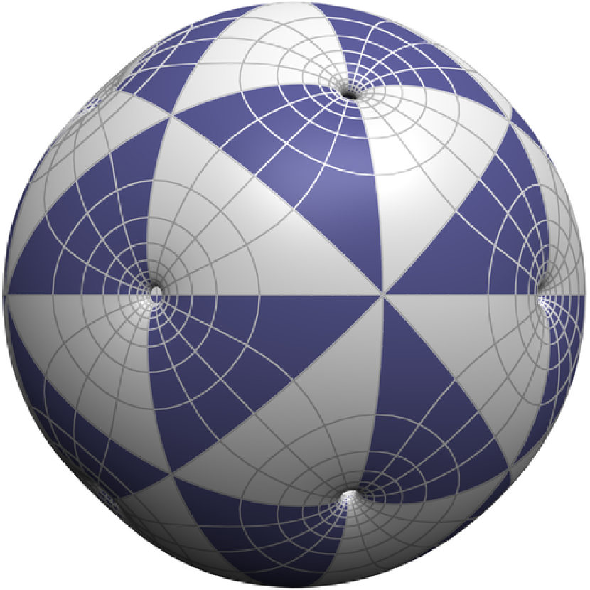
(a) alternate octahedron

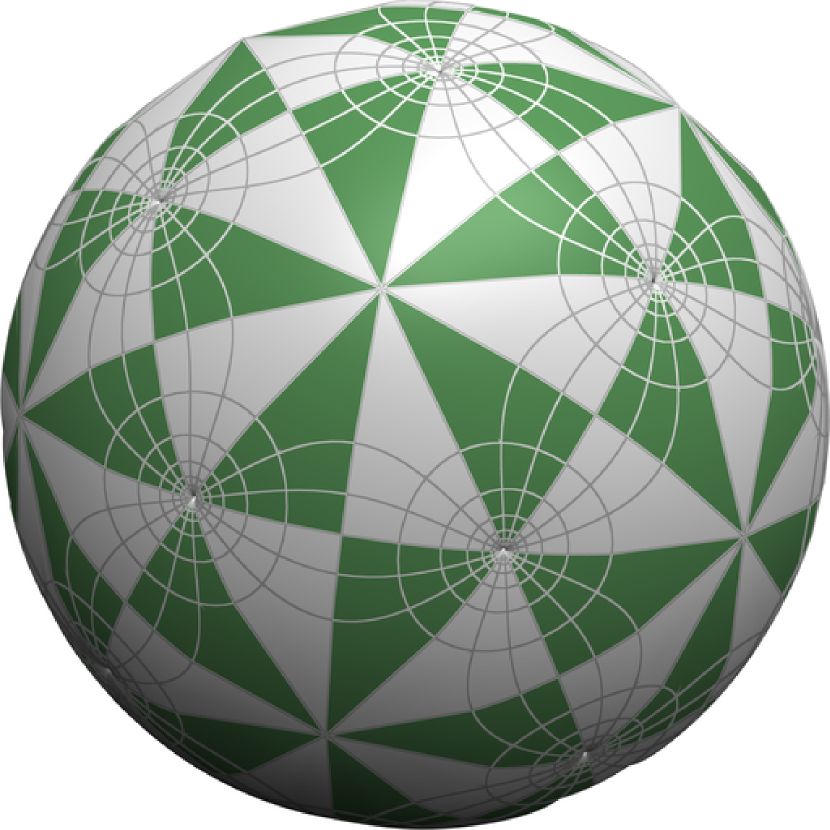
(b) icosahedron

(c) dodecahedron

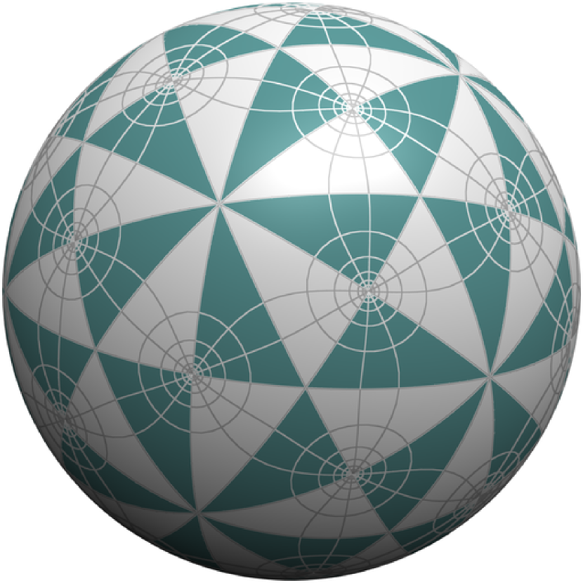
(d) alternate icosahedron

Figure 27. Minimal surfaces in $\mathbb{S}^{3}$ with Platonic symmetry

3.5.3. Building the surface

In general the position of the surface in space is not controlled, so to build the surface it must first be put into a standard position, where a group of standard reflections can be applied. To do so, compute the four generating reflections $R_{k}$ in the isometry group $\mathrm{Iso}\,\mathbb{R}^{3}$ of $\mathbb{R}^{3}$. Conjugate them to standard reflections $S_{k}$ via $CR_{k}C^{-1}=S_{k}$. Then the surface after being moved via $x\mapsto Cx$ has the standard reflections $S_{k}$ as symmetries.

3.5.4. The bulge count for families of CMC surfaces

The surfaces constructed in this paper allow for non-trivial 1-parameter deformations within the space of CMC surfaces with the same combinatorics. A natural question, also considered by [8], is whether different surfaces with the same combinatorics, but which swap neck and bulge, belong to the same family of CMC surfaces, for example figure 1a-b, and figure 3a-b. It turns out that these examples belong to different families. We denote by a leg of the surface a cylindrical piece obtained from the trajectories of the Hopf differential, that is from the curvature line parametrisation. Although the images are labeled according to whether there are bulges or necks where the legs meet, in this section we rather count the number of bulges on each leg.

We show that this number is an invariant in the case of surfaces without ends. Note that in this case, there is a covering $\Sigma\to\mathbb{C}\mathrm{P}^{1}$ by a compact Riemann surface $\Sigma$ on which the pullback of the DPW potential has only apparent singularities. Phrased differently, $\Sigma$ is the surface on which the first and second fundamental forms are well-defined and smooth, that is for compact CMC surfaces in the 3-sphere, $\Sigma$ is just the underlying Riemann surface, and in the case of periodic CMC surfaces in $\mathbb{R}^{3}$, $\Sigma$ is the Riemann surface quotient of the CMC surface by the translational symmetries.

We construct surfaces starting from Delaunay cylinders by deforming the eigenvalues $\nu_{i}.$ In the case of cylinders without umbilics, all four eigenvalues are $\nu_{i}=\tfrac{1}{4}.$ At the starting point, $\Sigma$ is a torus and the relevant moduli space of flat connections $\nabla$ on $\Sigma$ has only reducible points. The underlying holomorphic bundles (equipped with the $(0,1)$-parts $\bar{\operatorname{\partial\!}}^{\nabla}$ of the connections) are semistable, i.e. if they admit holomorphic line subbundles of degree 0. A holomorphic structure (on a rank 2 bundle over a compact Riemann surface of degree 0) is called unstable if there exist a holomorphic line subbundle of positive degree and they are called stable if every holomorphic line subbundle has negative degree. This notion is relevant to us since an unstable holomorphic structure does not admit a flat unitary connection. Spectral parameters $\lambda$ at which the holomorphic structure is unstable are isolated in the spectral plane. Moreover, for CMC surfaces based on quadrilaterals, the number of those values of spectral parameters within a bounded region is always finite and can only change during a deformation by values crossing the boundary of that region. Values of the spectral parameter at which the holomorphic structure is unstable cannot cross the unit circle, as the connections on the unit circle are unitary. For the initial torus the bundle is semistable for all spectral values. The number of values at which the holomorphic bundle becomes unstable within infinitesimal deformation of the eigenvalues $\nu_{i}$ can be identified with the number of bulges on the leg of the initial Delaunay cylinder; for more details see [12]. Actually this number coincides with the number of zeros of the holomorphic function $x$ in (3.2) inside the unit circle; see also [11, 15]

4. Fuchsian DPW potentials

The aim of this section is to prove the existence of Fuchsian DPW potentials of the form (3.1) for CMC quadrilaterals without Delaunay ends. This generalizes previous work by the second author [14] for the Lawson genus 2 surface. Similar results have been obtained by Manca [19]. Our arguments are more geometric and prove the existence of a Fuchsian potential on a 4-punctured sphere for all surfaces obtained by CMC quadrilaterals.

16cm(14.5cm,7.5cm)

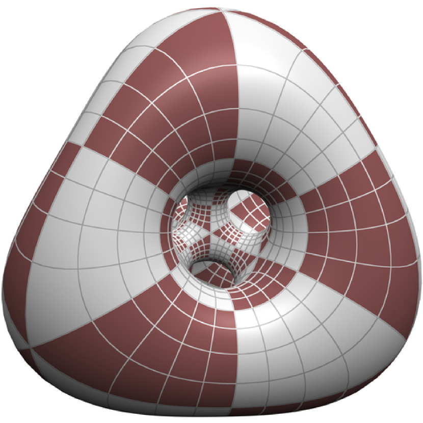
(a) $5$-cell

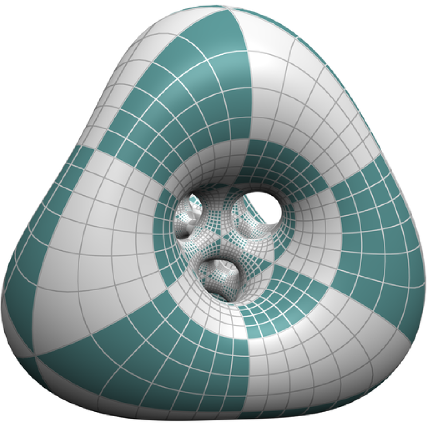
(b) $16$- or $8$-cell

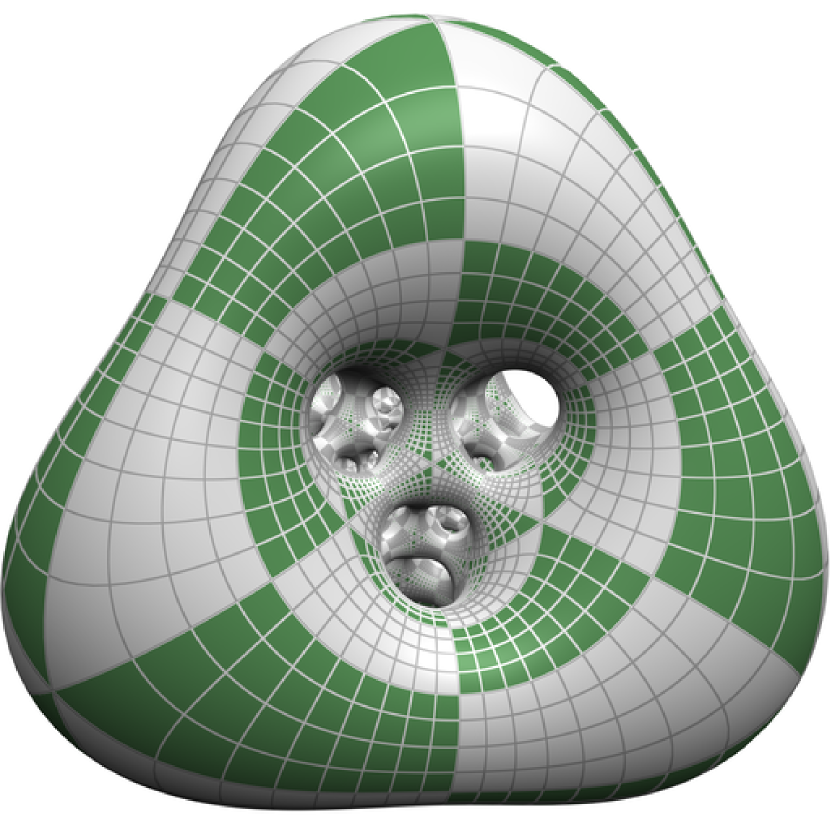
(c) $600$- or $120$-cell

Figure 28. Minimal surfaces in $\mathbb{S}^{3}$ with $n$-cell symmetry

4.1. Setup

Let $f\colon\Sigma\to M$ (where $M\in\{\mathbb{S}^{3},\mathbb{R}^{3}\}$) be a complete CMC surface without Delaunay ends. Assume that $f$ is build from a fundamental piece $P$ by the group $G$ generated by the reflections across totally geodesic subspaces along geodesic arcs contained in $P$. Assume that $P$ has the topology of a (closed) disc.

The surface $f$ is equivariant with respect to the (discrete) group $G$ acting on $\Sigma$ by conformal transformations and on the ambient space $M$ by a representation $\rho$ into the space of isometries. Let $G^{o}\subset G$ be the subgroup of orientation preserving (i.e. holomorphic) symmetries on $\Sigma$.

4.2. Local theory

The first step in our derivation of a Fuchsian DPW potential is the converse of theorem 2.5. This means that at fixed points of a rotational symmetry there always exists DPW potentials with Fuchsian singularity on the quotient.

Let $p\in\Sigma$ be a fixed point of some rotation given by an element in $G^{o}$. Then there exists $k\in\mathbb{N}$ and $g\in G^{o}$ of order $k$ such that $g(p)=p$ and such that for any $h\in G^{o}$ with $h(p)=p$ there exists $l\in\mathbb{N}$ with $g^{l}=h$.

Lemma 4.1.

There exists $D\in{\mathrm{SU}}_{2}{}$ of order $2k$ and a local DPW potential $\eta$ for $f$ on an open $g$-invariant neighbourhood of $p$ such that

(4.1) $$g^{*}\eta=D\eta D^{-1}\,\,\,.$$

Proof.

Consider Dorfmeister’s normalized potential (see for example [29]) which takes the form

(4.2) $$\eta^{nor}=\begin{bmatrix}0&\lambda^{-1}f(z,0)\\ \frac{q}{f(z,0)}&0\end{bmatrix}dz$$

where $z$ is a local holomorphic coordinate centered in $p$ such that $g^{*}z=e^{\frac{2\pi i}{k}}z$, $Q=q(dz)^{2}$ is the Hopf differential and $f(z,w)$ is a holomorphic function such that $f(z,\bar{z})dzd\bar{z}$ is the induced metric of the surface. As $g^{*}dz=e^{\frac{2\pi\mathbbm{i}}{k}}dz$ and $g^{*}d\bar{z}=e^{\frac{2\pi i}{k}}d\bar{z}$ the result follows. ∎

Proposition 4.2.

There exists a local meromorphic DPW potential of $f$ on $\Sigma/G^{o}$ with a Fuchsian singularity at $p\mod G^{o}$. The eigenvalues of the residue are $\pm\frac{1}{2k},$ independently of $\lambda$, where $k$ is the order of the stabilizer group of $p$.

Likewise, there exists a local meromorphic DPW potential of $f$ on $\Sigma/G^{o}$ with Fuchsian singularity at $p\mod G^{o}$ such that the eigenvalues of the residue are $\pm\frac{k-1}{2k}$.

Proof.

Consider $w=z^{k}$ which is a holomorphic coordinate centered at $p\mod G^{o}\in\Sigma/G^{o}$. Consider the positive gauge $e=\operatorname{diag}{(\sqrt{z},\frac{1}{\sqrt{z}})}$ of $\operatorname*{spin}$ $-1$. Then

(4.3) $$(d+\eta^{nor}).e=d+e^{-1}de+e^{-1}\eta^{nor}e$$

is a well-defined meromorphic DPW potential with apparent Fuchsian singularity at $p$. As this potential is clearly invariant under pull-back by $g$ we have proven the first part of the proposition.

For the second part and $k=2l+1$ consider the gauge $\tilde{e}=\operatorname{diag}{(z^{-l},z^{l})}$ while for $k=2l$ consider the gauge $\tilde{e}=\operatorname{diag}{(z^{-l+\tfrac{1}{2}},z^{l-\tfrac{1}{2}})}$, and proceed as in the first part of the proof. ∎

4.3. Global theory

Our aim is to construct a DPW potential on the $\Sigma/G^{o}$. Recall that by assumption the fundamental piece $P$ of the Riemann surface $\Sigma$ is of the topological type of a disc.

Lemma 4.3.

The Riemann surface $\Sigma/G^{o}$ is the projective line.

Proof.

By the Riemann mapping theorem there exists a holomorphic map from $P$ to the unit disc. Schwarzian reflection yields a holomorphic map from $\Sigma$ to $\mathbb{C}\mathrm{P}^{1}$, branched at the fixed points of $G^{o}$. By its construction, this map is invariant under $G^{o}$. ∎

For simplicity of the arguments, we will assume that $n$ is even in the following.

Lemma 4.4.

Let $n$ be even. There exists a unitary potential $\mu$ on the $n$-punctured Riemann sphere such that

• $\mu$ is singular exactly at the branch values of $\Sigma\to\Sigma/G^{o}=\mathbb{C}\mathrm{P}^{1};$

• the pull-back of $\mu$ generates $f$ on the covering $\Sigma$.

Proof.

Let $\{z_{1},\dots,z_{n}\}\subset\mathbb{C}\mathrm{P}^{1}$ be the branch values of $\Sigma\to\Sigma/G^{o}=\mathbb{C}\mathrm{P}^{1}$ and $S\subset\Sigma$ its preimage. Denote the reflection planes of the fundamental piece by $P_{0},\dots,P_{n-1},$ with outward oriented unit normals $N_{0},\dots,N_{n-1},$ respectively, such that

(4.4) $$z_{m}\in P_{m-1}\cap P_{m}\quad\forall m\in\{1,\dots,n\}\,\,\,.$$

Denote by $g_{m}$ the compositions of the reflection across $P_{m-1}$ and $P_{m}$. Then $G^{0}$ is generated by $\{g_{m}\mid\,m\in\{1,\dots,n\}\}$.

Let $M$ be euclidean 3-space or the 3-sphere, and let $d=3$ and $d=4$ accordingly, so that $\mathrm{Iso}(M)={\mathrm{SO}}_{4}{\mathbb{R}}$ or $\mathrm{Iso}(M)={\mathrm{SO}}_{3}{\mathbb{R}}\ltimes\mathbb{R}^{3}$.

Consider the group

(4.5) $$H\subset{\mathrm{Spin}}_{n}{\times}\mathrm{Iso}(M)$$

generated by the elements

(4.6) $$\hat{g}_{m}:=(N_{m}\cdot N_{m-1},g_{m}),\quad m=1,\dots,n$$

where $\cdot$ denotes Clifford multiplication. This gives a group extension

(4.7) $$\{\text{id}\}\to\mathbb{Z}_{2}\to H\to G^{0}\to\{\text{id}\}\,\,\,.$$

Note that $\hat{g}_{m}$ has order $2k$ if $g_{m}$ has order $k$. Similarly, since $n$ is even, the product $\hat{g}_{n}\dots\hat{g}_{1}$ is trivial. Consequently, we have a representation

(4.8) $$h\colon\pi_{1}(\mathbb{C}\mathrm{P}^{1}\setminus\{z_{1},\dots,z_{n}\},*)\to H\,\,\,.$$

As

(4.9) $$\Sigma\setminus S\to\mathbb{C}\mathrm{P}^{1}\setminus\{z_{1},\dots,z_{n}\}$$

is a (unbranched) covering, the fundamental group of $\Sigma\setminus S$ (with appropriate base point) is a subgroup of the first fundamental group of $\mathbb{C}\mathrm{P}^{1}\setminus\{z_{1},\dots,z_{n}\}$ with corresponding base point. By construction, the induced representation of $\pi_{1}(\Sigma\setminus S,*)\to G^{0}$ is trivial, and the induced representation of $h$ takes values in

(4.10) $$\mathbb{Z}_{2}=\mathbb{Z}_{2}\times\{\text{id}\}\subset{\mathrm{Spin}}_{d}{\times}\mathrm{Iso}(M)$$

such that a simple closed curve around any one of the points in $S$ is mapped to the non-trivial element in $\mathbb{Z}_{2}$.

16cm(14.5cm,7.5cm)

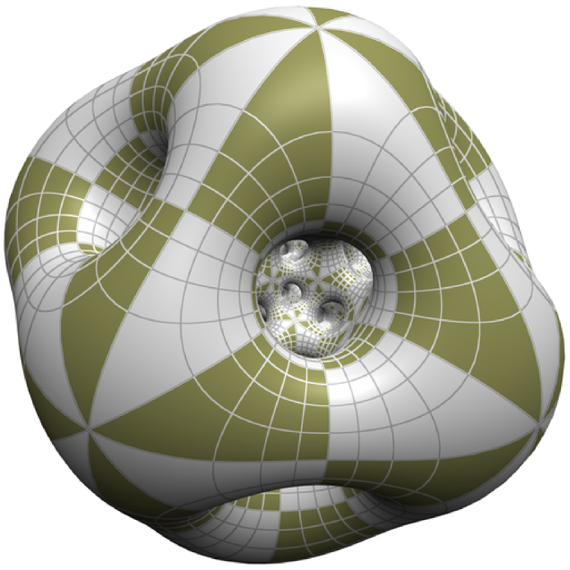
(a) $24$-cell

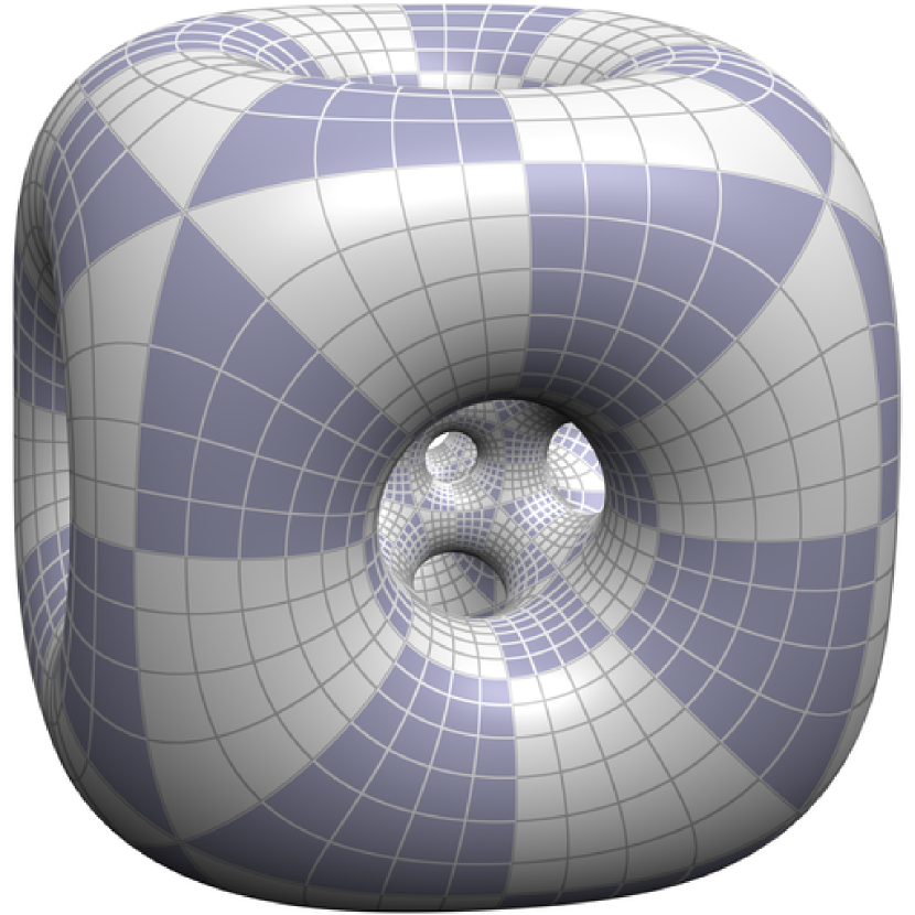
(b) $16$- or $8$-cell

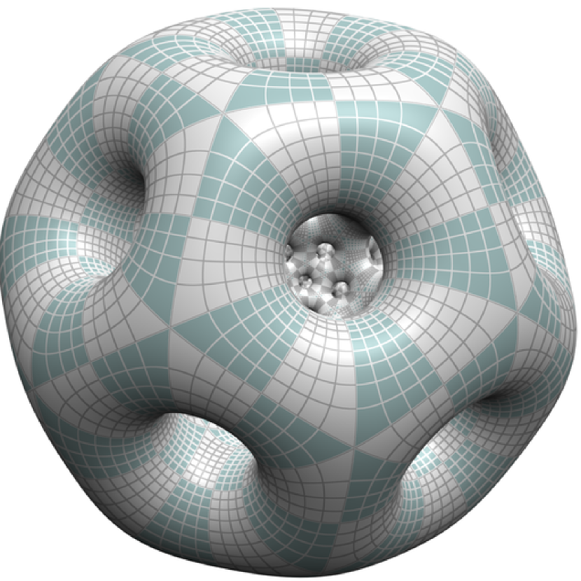
(c) $600$- or $120$-cell

Figure 29. Minimal surfaces in $\mathbb{S}^{3}$ with $n$-cell symmetry

By Riemann surface covering theory, we obtain a 2-fold covering

(4.11) $$\hat{\Sigma}\to\Sigma\,\,\,,$$

branched over the points in $S$, with an action of $H$ by holomorphic automorphisms on $\hat{\Sigma}$ such that

(4.12) $$\hat{\Sigma}\to\hat{\Sigma}/H=\mathbb{C}\mathrm{P}^{1}$$

is branched over $\{z_{1},\dots,z_{n}\}$. Denote its preimage of $S$ by $\hat{S}\subset\hat{\Sigma}$. Note that $H$ acts faithfully on $\hat{\Sigma}\setminus\hat{S}$.

Consider the pull-back $\omega$ on $\hat{\Sigma}$ of the unitary potential $\eta=F^{-1}\mathrm{d}F$ of $f$. Note that, for minimal $f\colon\Sigma\to\mathbb{S}^{3}$ the unitary potential is given by

(4.13) $$\eta=\lambda^{-1}\Phi+\Phi-\Phi^{*}-\lambda\Phi^{*}$$

where

(4.14) $$\Phi=\tfrac{1}{2}(f^{-1}df)^{1,0}\quad\text{and}\quad\Phi^{*}=\tfrac{1}{2}(f^{-1}df)^{0,1}$$

and similarly for CMC surfaces $f\colon\Sigma\to\mathbb{R}^{3}$. Let $\pi\colon H\to{\mathrm{SU}}_{2}{}$ be the projection to the rotational part of the symmetry. From the construction (4.13) of the unitary potential,

(4.15) $$h^{*}\eta_{\lambda}=\eta_{\lambda}.\pi(h)$$

for a holomorphic automorphism $h\in H$ (where, on the right hand side, the gauge action of the constant matrix $\pi(h)$ is given by conjugation).

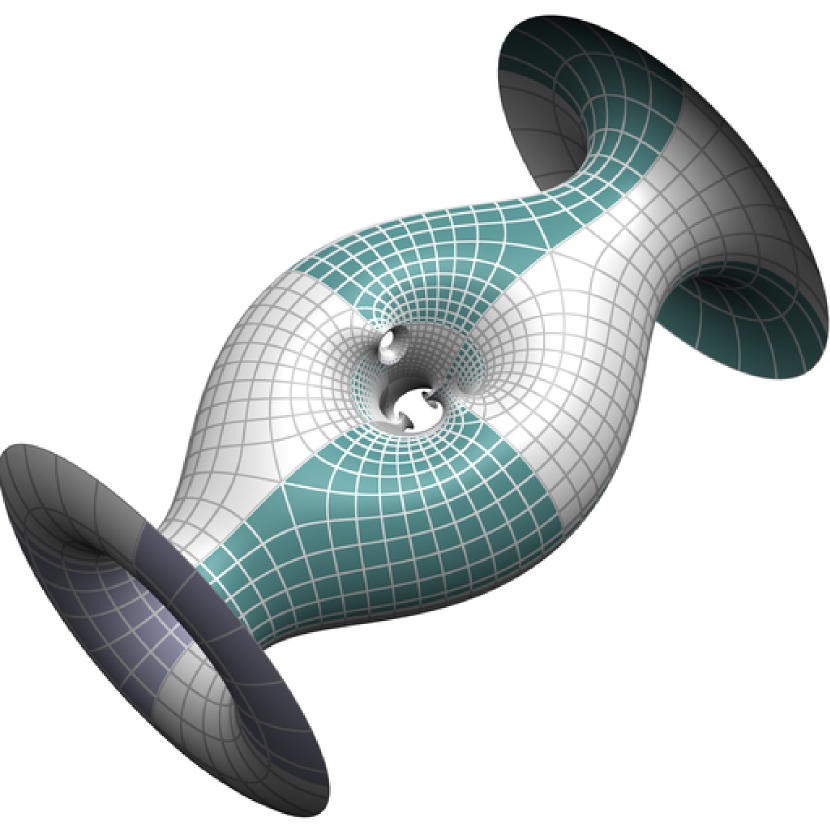
16cm(14.5cm,20.2cm) (a) torus 8 Figure 30. Minimal torus in $\mathbb{S}^{3}$ with Delaunay ends

Consider the free action of $H$ on $\hat{\Sigma}\setminus\hat{S}\times\mathbb{C}^{2}$ given by

(4.16) $$(p,v).h=(p.h,\pi(h^{-1})(v))\,\,\,.$$

The quotient

(4.17) $$V=(\hat{\Sigma}\setminus\hat{S}\times\mathbb{C}^{2})/H$$

is a trivial smooth vector bundle of rank 2 over $\mathbb{C}\mathrm{P}^{1}\setminus\{z_{1},\dots,z_{n}\}$. We claim that the unitary potential $\omega$ yields a well-defined potential $\mu$ on this vector bundle: in fact, the connection 1-form acts on $[p,v]\in(\hat{\Sigma}\setminus\hat{S}\times\mathbb{C}^{2})/H$ as

(4.18) $$[p,\omega_{p}(v)]$$

which is well-defined since

(4.19) $$(p,\omega_{p}(v)).h=(ph,h^{-1}\omega_{p}hh^{-1}(v))=(ph,\omega_{ph}(h^{-1}v))\,\,\,.$$

∎

Proposition 4.5.

Let $n$ be even. There exist a meromorphic DPW potential $\xi$ on $\mathbb{C}\mathrm{P}^{1}$ with simple poles at $z_{1},\dots,z_{n}$ and possible apparent singularity at $z=\infty$.

Proof.

From lemma 4.4 we obtain a unitary potential $\mu$ on the $n$-punctured sphere. Let $l\in\{1,\dots,n\}$. By proposition 4.2 there exist a DPW gauge locally well-defined on a punctured disc around $z_{l}$ which gauges $\mu$ into a meromorphic potential with a Fuchsian singularity at $z_{l}$. Of course, the holomorphic structures (i.e. the $(0,1)$-part) of a meromorphic potential extends to the singular points. Note that these gauges are well-defined (i.e. have $\operatorname*{spin}$ 1) as we have chosen the representation $s\colon\pi_{1}(\Sigma\setminus S,\mathbb{Z}_{2})$ to have local monodromy $-1$ around every point in $S$.

Using these gauges as cocycles, we obtain a holomorphic $\mathbb{C}^{*}$-family of flat ${\mathrm{SL}}_{2}{\mathbb{C}}$-connections $d+\hat{\mu}$ with the following properties:

• the induced family of holomorphic structures extends to $\lambda=0$ to give a holomorphic rank 2 bundle $\mathcal{E}_{0}\to\mathbb{C}\mathrm{P}^{1}$ with trivial holomorphic determinant;

• the connections $d+\hat{\mu}$ have Fuchsian singularities with $\lambda$-independent eigenvalues $\pm\tfrac{1}{2k};$

• the complex linear part of the family of connections has a first order pole at $\lambda=0$, i.e., $\lambda\mapsto\lambda(\hat{\mu})^{1,0}(\lambda)$ extends to $\lambda=0$.

Note that all bundles have trivial determinant. Hence, by the Birkhoff-Grothendieck theorem, the bundle type of $\mathcal{E}_{0}$ is $\mathcal{O}(d)\oplus\mathcal{O}(-d)$ for some $d\in\mathbb{N}$.

First consider the case $d=0$. Then, the bundle type $\mathcal{E}_{\lambda}$ is locally constant on an open disc near $\lambda=0$. In particular, there exists a smooth positive family of gauge transformations $g_{\lambda}$ (holomorphic in $\lambda$) such that

(4.20) $$((d+\hat{\mu}).g_{\lambda})^{0,1}=d^{0,1}$$

is the trivial holomorphic structure on the rank 2 vector bundle $\mathbb{C}^{2}\to\mathbb{C}\mathrm{P}^{1}$. Thus

(4.21) $$d+\xi:=(d+\hat{\mu}).g_{\lambda}$$

is the meromorphic DPW potential which has only Fuchsian singularities and no apparent singularity at $\infty$.

Let $d>0$. Let $z\colon\mathbb{C}\mathrm{P}^{1}\setminus\{\infty\}\to\mathbb{C}$ be an affine holomorphic coordinate and assume without loss of generality that $z_{l}\neq\infty\quad\forall\;l\in\{1,\dots,n\}$. There exists an integer $0\leq s\leq d$ such that on a punctured disc $\mathcal{D}\setminus\{0\}$ around $\lambda=0$ all bundles are of the holomorphic type $\mathcal{O}(s)\oplus\mathcal{O}(-s)$. By the family version of Birkhoff-Grothendieck, there exists a holomorphic function $r\colon\mathcal{D}\to\mathbb{C}$ with $r(0)=0$ such that the holomorphic bundle $((d+\hat{\mu}).g_{\lambda})^{0,1}$ has the cocycle (for the covering $\mathcal{U}_{+}:=\mathbb{C},\mathcal{U}_{-}:=\mathbb{C}P^{1}\setminus\{\infty\}$ of $\mathbb{C}\mathrm{P}^{1}$)

(4.22) $$\begin{bmatrix}z^{-d}&z^{s}r(\lambda)\\ 0&z^{d}\end{bmatrix}=\begin{bmatrix}r(\lambda)z^{s}&0\\ z^{d}&\tfrac{1}{r(\lambda)}z^{-s}\end{bmatrix}\begin{bmatrix}\tfrac{1}{r(\lambda)}z^{-d-s}&1\\ -1&0\end{bmatrix}\,\,\,,$$

where the equality obviously holds only for $r(\lambda)\neq 0$. Again, there exists a DPW gauge $g_{\lambda}$ which gauges $\mathcal{E}_{\lambda}$ into the above form (4.22). This means that there exists a pair $(g^{+}_{\lambda},\,g^{-}_{\lambda})$ of DPW gauges on $\mathcal{U}_{+}$ respectively $\mathcal{U}_{-}$ which differ by the gauge (4.22) and gauge $(d+\hat{\mu})^{0,1}$ on $\mathcal{U}_{\pm}$ to the trivial holomorphic structure on $\mathbb{C}^{2}\to\mathcal{U}_{\pm}$. Then,

(4.23) $$(d+\hat{\mu}).g^{+}_{\lambda}=:d+\xi$$

yields the meromorphic potential $\xi$ with Fuchsian singularities at $z_{k}$ and an apparent singularity at $\infty$. ∎

4.3.1. CMC quadrilaterals

Finally, we consider the case of CMC quadrilaterals, i.e., $n=4$. We show that these are always determined by a Fuchsian DPW potential (3.1), which, assuming an additional symmetry, is of the form (3.2).

Lemma 4.6.

For $n=4$ the bundle type of $\mathcal{E}_{0}$ is either trivial or $\mathcal{O}(1)\oplus\mathcal{O}(-1)\to\mathbb{C}\mathrm{P}^{1}$.

Proof.

Assume the bundle type at $\lambda=0$ is $\mathcal{O}(d)\oplus\mathcal{O}(-d)\to\mathbb{C}\mathrm{P}^{1}$ for some $d>1$. The Higgs field $\Phi:=\text{res}_{\lambda=0}\xi$ is a meromorphic section of the bundle

(4.24) $$K\otimes\text{End}_{0}(\mathcal{E}_{0})\to\mathbb{C}\mathrm{P}^{1}$$

where $K=\mathcal{O}(-2)$ is the canonical bundle of $\mathbb{C}\mathrm{P}^{1}$ and $\text{End}_{0}(\mathcal{E}_{0})$ denotes the trace-free endomorphisms of $\mathcal{E}_{0}$. Moreover, $\Phi$ is nilpotent as the immersion is conformal, has at most simple poles at $z_{1},\dots,z_{4}$ by construction and does not vanish on $\mathbb{C}\mathrm{P}^{1}$ as $f$ is an immersion. Using the decomposition $\mathcal{E}_{0}=\mathcal{O}(d)\oplus\mathcal{O}(-d)$ the Higgs field is of the form

(4.25) $$\Phi=\begin{bmatrix}a&b\\ c&-a\end{bmatrix}$$

where $a,b,c$ are meromorphic sections in $\mathcal{O}(-2)$, $\mathcal{O}(-2+2d),\mathcal{O}(-2-2d),$ respectively, with at most simple poles at $z_{1},\dots,z_{4}$. Hence $c=0$. As $\Phi$ is nilpotent $a=0$ as well. For $d>1$, $-2+2d>0$ and $b$ would have a zero contradicting the fact that $\Phi$ is nowhere vanishing. ∎

Theorem 4.7.

Let $f$ be a complete CMC surface without Delaunay ends in $\mathbb{S}^{3}$ or $\mathbb{R}^{3}$. If $f$ is built from a CMC quadrilateral in a fundamental tetrahedron of a tessellation of the ambient space then it is obtained from a Fuchsian DPW potential (3.1) on the 4-punctured sphere.

Proof.

We give a proof by contradiction. Assume that the bundle type at $\lambda=0$ is

(4.26) $$\mathcal{E}_{0}=\mathcal{O}(-1)\oplus\mathcal{O}(1)\,\,\,.$$

By the proof of proposition 4.2 the nilpotent $\lambda^{-1}$-part $\Phi=\xi_{-1}$ of the meromorphic potential has no zeros, and poles of order $1$ at the 4 branch points $z_{1},\dots,z_{4}$. Thus, with respect to (4.26), it must be of the form

(4.27) $$\Phi=\begin{bmatrix}0&s_{-D}\\ 0&0\end{bmatrix}$$

where $s_{-D}\in\mathcal{M}(\mathbb{C}\mathrm{P}^{1},\mathcal{O}(-4))$ is the unique meromorphic section (up to scaling) with simple poles at $D=z_{1}+\dots+z_{4}$. Moreover, the positive eigenvalues $\nu_{i}$ of the residues of the connections are contained in the respective kernels of the residues of $\xi_{-1}$. This equips $\mathcal{E}_{0}$ with a parabolic structure (see for example [21, 26, 23, 11, 3] for definitions and further references) which is unstable. We denote the parabolic bundle also by $\mathcal{E}_{0}$. The pair $(\mathcal{E}_{0},\Phi)$ is a stable strongly parabolic Higgs pair. Note that

(4.28) $$\sum_{i}\nu_{i}<1\,\,\,.$$

It is easy to see (compare with [11]) that $(\mathcal{E}_{0},\Phi)$ is the only stable strongly parabolic Higgs pair with nilpotent Higgs field on the 4-punctured sphere with unstable underlying parabolic bundle. Consider the compact Riemann surface $X\to\mathbb{C}\mathrm{P}^{1}$ on which the rotational symmetry is trivial. Its Fuchsian monodromy (given by uniformization) corresponds by the Hitchin-Kobayashi correspondence to a stable nilpotent Higgs pair

(4.29) $$\biggl{(}S^{*}\oplus S\,\,\,,\ \begin{bmatrix}0&1\\ 0&0\end{bmatrix}\biggr{)}\,\,\,,$$

where $S^{2}=K_{X}$. Its underlying holomorphic structure is unstable. As the rotational symmetries act on $X$ we obtain, in the same manner as for $f$, an strongly parabolic nilpotent Higgs pair with underlying parabolic structure. As the holomorphic structure is unstable, the parabolic structure must be unstable as well; see [2], and hence it must be $(\mathcal{E}_{0},\Phi)$. Thus, the holomorphic Higgs pair of $f$, i.e., $(\partial^{\nabla},\Phi)$ would be gauge equivalent to $(S^{*}\oplus S,\bigl{[}\begin{smallmatrix}0&1\\ 0&0\end{smallmatrix}\bigr{]})$. This is only possible if the Hopf differential of the minimal (respectively CMC) surface vanishes (compare with [14, sections 2 and 3]), which gives a contradiction. ∎

Finally, we show under which conditions the Fuchsian DPW potential $\xi$ can be gauged into the form (3.2).

Note that a Fuchsian potential for a CMC quadrilateral defining a compact embedded CMC surface cannot be adapted if all the 4 positive eigenvalues of the residues are contained in $(0,\tfrac{1}{4})$.

Corollary 4.8.

Assume that the potential of theorem 4.7 has equal pairs of eigenvalues. Then, there exist a coordinate change and a gauge such that the potential is of the form (3.2).

Proof.

We only sketch the proof. Assume that the eigenvalues at $z_{0}$ and $z_{1}$, respectively $z_{2}$ and $z_{3}$ are equal. First, apply a so-called flip gauge which flips the eigenvalues at $z_{2}$ and $z_{3}$ by adding $\mp\tfrac{1}{2}$. This can be achieved by conjugating the potential by a DPW gauge which is constant in $z$ such that the residues at $z_{2}$ and $z_{3}$ are lower respectively upper triangular, and then gauge with $\operatorname{diag}(\sqrt{\tfrac{z-z_{2}}{z-z_{3}}},\sqrt{\tfrac{z-z_{3}}{z-z_{2}}})$. Denote the residues of the potential $\tilde{\xi}$ obtained in this way by $R_{k},$ and find $T$ such that $R_{3}=TD^{-1}T^{-1}R_{2}TDT^{-1}$. Then, $T^{-1}\tilde{\xi}T$ turns out to be of the form (3.2). ∎

References

- [1] D.V. Anosov and A.A. Bolibruch, The Riemann-Hilbert problem, Aspects math. E22, Braunschweig: Vieweg and Sohn, 1994.
- [2] I. Biswas, Parabolic bundles as orbifold bundles, Duke Math. J. 88 (1997), no. 2, 305–325.
- [3] I. Biswas, S. Dumitrescu, and S. Heller, Irreducible flat sl(2,r)-connections on the trivial holomorphic bundle, arXiv:2003.06997; to appear in Journal de Math. Pures et Appl., 2020.
- [4] A. Bobenko, Constant mean curvature surfaces and integrable equations, Uspekhi Mat. Nauk, Russian Math. Surveys 46 (1991), no. 4, 3–42.
- [5] DGD-Gallery, www.discretization.de/gallery/.
- [6] J. Dorfmeister, F. Pedit, and H. Wu, Weierstrass type representation of harmonic maps into symmetric spaces, Comm. Anal. Geom. 6 (1998), no. 4, 633–668.
- [7] A.S. Fokas, A.R. Its, A.A. Kapaev, and V.Yu Novokshenov, Painlevé transcendents: The Riemann-Hilbert approach, Math. Surveys and Monographs, vol. 128, AMS, Providence, 2006.
- [8] K. Große-Brauckmann, New surfaces of constant mean curvature, Math. Z. 214 (1993), no. 4, 527–565.
- [9] K. Grosse-Brauckmann, Triply periodic minimal and constant mean curvature surfaces, Interface Focus 2 (2012), 582–588.
- [10] K. Große-Brauckmann and K. Polthier, Constant mean curvature surfaces derived from Delaunay’s and Wente’s examples, Visualization and Mathematics (1997), 119–134.
- [11] L. Heller and S. Heller, Abelianization of Fuchsian systems on a 4-punctured sphere and applications, J. Symplectic Geom. 14 (2016), no. 4, 1059–1088.
- [12] L. Heller, S. Heller, and N. Schmitt, Navigating the space of symmetric CMC surfaces, J. Differential Geom. 110 (2018), no. 3, 413–455.
- [13] L. Heller, S. Heller, and M. Traizet, Area estimates for high genus Lawson surfaces via dpw, arXiv 1907.07139, 2019.
- [14] S. Heller, Lawson’s genus two surface and meromorphic connections, Math. Z. 274 (2013), no. 3-4, 745–760.
- [15] S. Heller and N. Schmitt, Deformations of symmetric CMC surfaces in the 3-sphere, Experimental Mathematics 24 (2015), no. 01.
- [16] H. Karcher, U. Pinkall, and I. Sterling, New minimal surfaces in , J. Differential Geom. 28 (1988), no. 2, 169–185.
- [17] M. Kilian, W. Rossman, and N. Schmitt, Delaunay ends of constant mean curvature surfaces, Compos. Math. 144 (2008), no. 1, 186–220.
- [18] H. Lawson, Jr., Complete minimal surfaces in , Ann. of Math. (2) 92 (1970), 335–374.
- [19] B. Manca, Dpw potentials for compact symmetric CMC surfaces in, J. Geom. Phys. 156 (2020), 103791, 16.
- [20] I. McIntosh, Global solutions of the elliptic D periodic Toda lattice, Nonlinearity 7 (1994), no. 1, 85–108.
- [21] V. Mehta and C. Seshadri, Moduli of vector bundles on curves with parabolic structures, Math. Ann. 248 (1980), no. 3, 205–239.
- [22] B. Oberknapp and K. Polthier, An algorithm for discrete constant mean curvature surfaces, Visualization and Mathematics, Ed: H.C. Hege, K. Polthier (1997), 141–161.
- [23] G. Pirola, Monodromy of constant mean curvature surface in hyperbolic space, Asian J. Math. 11 (2007), no. 4, 651–669.
- [24] A. Pressley and G. Segal, Loop groups, Oxford Mathematical Monographs, The Clarendon Press, Oxford University Press, New York, 1986, Oxford Science Publications.
- [25] N. Schmitt, M. Kilian, S. Kobayashi, and W. Rossman, Unitarization of monodromy representations and constant mean curvature trinoids in 3-dimensional space forms, J. Lond. Math. Soc. (2) 75 (2007), no. 3, 563–581.
- [26] C. Simpson, Harmonic bundles on noncompact curves, J. Amer. Math. Soc. 3 (1990), no. 3, 713–770.
- [27] M. Traizet, Construction of constant mean curvature -noids using the DPW method, J. Reine Angew. Math. 763 (2020), 223–249, arXiv:1709.00924.
- [28] by same author, Gluing Delaunay ends to minimal n-noids using the dpw method., Mathematische Annalen 377 (2020), no. 3, 1481–1508.
- [29] H. Wu, A simple way for determining the normalized potentials for harmonic maps, Ann. Global Anal. Geom. 17 (1999), 189–199.