Reducing the Amortization Gap in Variational Autoencoders:
A Bayesian Random Function Approach

Abstract

Variational autoencoder (VAE) is a very successful generative model whose key element is the so called amortized inference network, which can perform test time inference using a single feed forward pass. Unfortunately, this comes at the cost of degraded accuracy in posterior approximation, often underperforming the instance-wise variational optimization. Although the latest semi-amortized approaches mitigate the issue by performing a few variational optimization updates starting from the VAE’s amortized inference output, they inherently suffer from computational overhead for inference at test time. In this paper, we address the problem in a completely different way by considering a random inference model, where we model the mean and variance functions of the variational posterior as random Gaussian processes (GP). The motivation is that the deviation of the VAE’s amortized posterior distribution from the true posterior can be regarded as random noise, which allows us to take into account the uncertainty in posterior approximation in a principled manner. In particular, our model can quantify the difficulty in posterior approximation by a Gaussian variational density. Inference in our GP model is done by a single feed forward pass through the network, significantly faster than semi-amortized methods. We show that our approach attains higher test data likelihood than the state-of-the-arts on several benchmark datasets.

1 Introduction

Variational Autoencoder (VAE) (Kingma & Welling, 2014; Rezende et al., 2014) is a very successful generative model where a highly complex deep nonlinear generative process can be easily incorporated. A key element of the VAE, the deep inference (a.k.a. encoder) network, can perform the test time inference using a single feed forward pass through the network, bringing significant computational speed-up. This feature, known as amortized inference, allows the VAE to circumvent otherwise time-consuming steps of solving the variational optimization problem for each individual instance at test time, required in the standard variational inference techniques, such as the stochastic variational inference (SVI) (Hoffman et al., 2013).

As suggested by the recent study (Cremer et al., 2018), however, the amortized inference can also be a drawback of the VAE, specifically the accuracy of posterior approximation by the amortized inference network is often lower than the accuracy of the SVI’s full variational optimization. There are two general approaches to reduce this amortization error. The first is to increase the network capacity of the inference model (e.g., flow-based models (Kingma et al., 2016; Tomczak & Welling, 2016)). The other direction is the so-called semi-amortized approach (Kim et al., 2018; Krishnan et al., 2018; Marino et al., 2018; Park et al., 2019), where the key idea is to use the VAE’s amortized inference network to produce a good initial distribution, from which a few SVI steps are performed at test time to further reduce the amortization error, quite similar in nature to the test time model adaptation of the MAML (Finn et al., 2017) in multi-task (meta) learning. Although these models often lead to improved posterior approximation, they raise several issues: Training the models for the former family of approaches is usually difficult because of the increased model complexity; the latter approaches inadvertently suffer from computational overhead of additional SVI gradient steps at test time.

In this paper, we propose a novel approach to address these drawbacks. We retain the amortized inference framework similar to the standard VAE for its computational benefits, but consider a random inference model. Specifically, the mean and the variance functions of the variational posterior distribution are a priori assumed to be Gaussian process (GP) distributed. There are two main motivations for this idea. The first one stems from the suboptimality of the VAE, where the estimated amortized inference network suffers from deviation from the true posteriors. This inaccuracy can be characterized by inherent uncertainty in the posterior approximation of the deterministic amortized inference network, suggesting the need for a principled Bayesian uncertainty treatment. The second intuition is that the deviation of the VAE’s variational posterior distributions from the true posteriors can be naturally regarded as random noise. Whereas the semi-amortized approaches perform extra SVI gradient updates at test time to account for this noise, we model the discrepancy using a Bayesian neural network (GP), resulting in a faster and more accurate amortized model via principled uncertainty marginalization. Another benefit of the Bayesian treatment is that our model can quantify the discrepancy in approximation, which can serve as useful indicators for goodness of posterior approximations.

The inference in our model is significantly faster than that of semi-amortized methods, accomplished by a single feed forward pass through the GP posterior marginalized inference network. We show that our approach attains higher test data likelihood scores than the state-of-the-art semi-amortized approaches and even the high-capacity flow-based encoder models on several benchmark datasets.

2 Background

Let ${\bf x}\in\mathcal{X}$ be an input data point and ${\bf z}\in\mathbb{R}^{d}$ be the $d$-variate latent vector. We consider the generative model:

$$p({\bf z})=\mathcal{N}({\bf z};{\bf 0},{\bf I}),\ \ \ p_{\bm{\theta}}({\bf x}|{\bf z})=\mathcal{N}({\bf x};{\bf g}_{\bm{\theta}}({\bf z}),\sigma_{\bf x}^{2}{\bf I}),$$ (1)

where ${\bf g}_{\bm{\theta}}:\mathbb{R}^{d}\rightarrow\mathcal{X}$ is a (deep) neural network with the weight parameters denoted by $\bm{\theta}$, and $\sigma_{\bf x}^{2}$ is the variance of the white noise. For the given data $\mathcal{D}=\{{\bf x}^{i}\}_{i=1}^{N}$, we maximize the data log-likelihood, $\sum_{i=1}^{N}\log p_{\bm{\theta}}({\bf x}^{i})$, with respect to $\bm{\theta}$ where $p_{\bm{\theta}}({\bf x})=\mathbb{E}_{p({\bf z)}}[p_{\bm{\theta}}({\bf x}|{\bf z})]$. Due to the infeasibility of evaluating the marginal log-likelihood exactly, the variational inference exploits the following inequality,

$$\log p_{\bm{\theta}}({\bf x})\geq\mathbb{E}_{q({\bf z}|{\bf x})}\big{[}\log p_{\bm{\theta}}({\bf x},{\bf z})-\log q({\bf z}|{\bf x})\big{]},$$ (2)

which holds for any density $q({\bf z}|{\bf x})$. The inequality becomes tighter as $q({\bf z}|{\bf x})$ becomes closer to the true posterior, as the gap equals $\textrm{KL}(q({\bf z}|{\bf x})||p_{\bm{\theta}}({\bf z}|{\bf x}))$. Then we adopt a tractable density family (e.g., Gaussian) $q_{\bm{\lambda}}({\bf z}|{\bf x})$ parametrized by $\bm{\lambda}$, and maximize the lower bound in (2) w.r.t. $\bm{\lambda}$. Since our goal is maximizing the log-marginal, $\log p_{\bm{\theta}}({\bf x})$, we also need to optimize the lower bound w.r.t. $\bm{\theta}$ together with $\bm{\lambda}$, either concurrently or in an alternating fashion.

Note that at current $\bm{\theta}$, the lower bound optimization w.r.t. $\bm{\lambda}$ needs to be specific to each input ${\bf x}$, and hence the optimal solution is dependent on the input ${\bf x}$. Formally, we can denote the optimum by $\bm{\lambda}^{*}({\bf x})$. The stochastic variational inference (SVI) (Hoffman et al., 2013) faithfully implements this idea, and the approximate posterior inference for a new input point ${\bf x}$ in SVI amounts to solving the ELBO optimization on the fly by gradient ascent. Although this can yield very accurate posterior approximation, it incurs computational overhead since we have to perform full variational optimization for each and every input ${\bf x}$. The VAE (Kingma & Welling, 2014) addresses this problem by introducing a deep neural network $\bm{\lambda}({\bf x};\bm{\phi})$ with the weight parameters $\bm{\phi}$ as a universal function approximator of the optimum $\bm{\lambda}^{*}({\bf x})$, and optimize the lower bound w.r.t. $\bm{\phi}$. This approach is called the amortized variational inference (AVI). Thus the main benefit of the VAE is computational speed-up as one can simply do feed forward pass through the inference network $\bm{\lambda}({\bf x};\bm{\phi})$ to perform posterior inference for each ${\bf x}$.

The recent study in (Cremer et al., 2018) raised the issue of the amortized inference in the VAE, where the quality of data fitting is degraded due to the approximation error between $\bm{\lambda}^{*}({\bf x})$ and $\bm{\lambda}({\bf x};\bm{\phi})$, dubbed the amortization error. To retain the AVI’s computational advantage and reduce the amortization error, there were attempts to take the benefits of SVI and AVI, which are referred to as semi-amortized variational inference (SAVI) (Kim et al., 2018; Marino et al., 2018; Krishnan et al., 2018). The key idea is to learn the amortized inference network to produce a reasonably good initial iterate for the follow-up SVI optimization, perhaps just a few steps. This warm-start SVI gradient ascent would be faster than full SVI optimization, and could reduce the approximation error of the AVI.

Although the inference in the SAVI is faster than SVI, it still requires gradient ascent optimization at test time, which might be the main drawback. The SAVI also suffers from other minor issues including how to choose the gradient step size and the number of gradient updates to achieve optimal performance-efficiency trade-off. In the next section we propose a novel approach that is much faster than the SAVI, avoiding gradient updates at test time and requiring only feed forward pass through a single network, and at the same time can yield more accurate posterior approximation.

3 Gaussian Process Inference Network

We start from the variational density of the VAE, but with slightly different notation, as follows:

$$q({\bf z}|{\bf x},{\bf f},{\bf h})=\mathcal{N}\big{(}{\bf z};{\bf f}({\bf x}),\textrm{Diag}({\bf h}({\bf x}))^{2}\big{)},$$ (3)

where ${\bf f},{\bf h}:\mathcal{X}\rightarrow\mathbb{R}^{d}$ are the mean and standard deviation functions of the variational posterior distribution. Note that if we model ${\bf f}$ and ${\bf h}$ as deterministic functions (neural networks) and optimize their weight parameters (i.e., point estimation), then it reduces to the standard VAE for which ${\bf f}$ and ${\bf h}$ constitute $\bm{\lambda}({\bf x};\bm{\phi})$. However, as discussed in the previous sections, such point estimates may be inaccurate, which implies that there must be inherent uncertainty in posterior approximation. To account for the uncertainty, we follow the Bayesian treatment; specifically we let ${\bf f}$ and ${\bf h}$ be independent random GP distributed functions a priori (Rasmussen & Williams, 2006),

$${\bf f}(\cdot) =[f_{1}(\cdot),...,f_{d}(\cdot)]^{\top}\sim\prod_{j=1}^{d}\mathcal{GP}(b_{j}(\cdot),k^{m}(\cdot,\cdot)),$$ (4)

$${\bf h}(\cdot) =[h_{1}(\cdot),...,h_{d}(\cdot)]^{\top}\sim\prod_{j=1}^{d}\mathcal{GP}(c_{j}(\cdot),k^{s}(\cdot,\cdot)).$$ (5)

Here ${\bf b}(\cdot)=[b_{1}(\cdot),...,b_{d}(\cdot)]^{\top}$, ${\bf c}(\cdot)=[c_{1}(\cdot),...,c_{d}(\cdot)]^{\top}$ are the GP mean functions which can be modeled by deep neural networks, and the GP covariance functions of ${\bf f}$ and ${\bf h}$ are denoted by $k^{m}$ and $k^{s}$, respectively, where we share the same covariance function across dimensions for simplicity.

Relation to the SAVI. Note that the GP-priored variational density model in (3–5) can be equivalently written as:

$$q({\bf z}|{\bf x},{\bf f},{\bf h})=\mathcal{N}\big{(}{\bf b}({\bf x})+{\bf f}({\bf x}),\textrm{Diag}({\bf c}({\bf x})+{\bf h}({\bf x}))^{2}\big{)},$$ (6)

where ${\bf f}$ and ${\bf h}$ now follow zero-mean Gaussian processes. If we view the VAE’s point estimate inference model as: $q({\bf z}|{\bf x})=\mathcal{N}\big{(}{\bf b}({\bf x}),\textrm{Diag}({\bf c}({\bf x}))^{2}\big{)}$, then (6) effectively models the discrepancy between the VAE’s $q({\bf z}|{\bf x})$ and the true posterior $p_{\bm{\theta}}({\bf z}|{\bf x})$ via stochastic noise models. Recall that in order to reduce this discrepancy, the semi-amortized approaches perform extra SVI gradient updates starting from ${\bf b}({\bf x})$ and ${\bf c}({\bf x})$ at test time on the fly. Instead, we aim to learn the discrepancy using Bayesian neural networks ${\bf f}$ and ${\bf h}$ (GP as a special case; see Sec. 3.1), resulting in a faster and more accurate amortized inference model by taking into account uncertainty in a principled manner.

For instance, the GP posterior $p({\bf f},{\bf h}|\mathcal{D})$ can predict the above-mentioned discrepancy accurately, while their variances (e.g., $\mathbb{V}(f({\bf x})|\mathcal{D})$) can serve as gauge that quantifies the degree of (instance-wise) uncertainty/difficulty in posterior approximation via the amortized inference network. To this end, we describe a reasonable likelihood model to establish a GP framework, and derive an efficient GP posterior inference algorithm in what follows.

3.1 Likelihood Model and GP Posterior Inference

To establish a valid Bayesian framework, we define a likelihood model, that is, the compatibility score of how each individual instance ${\bf x}\sim\mathcal{D}$ is likely to be generated under the given functions ${\bf f}$ and ${\bf h}$. A reasonable choice is the variational lower bound (2), which we denote as:

$$\mathcal{L}_{\bm{\theta}}({\bf f},{\bf h};{\bf x}):=\mathbb{E}_{q({\bf z}|{\bf x},{\bf f},{\bf h})}\big{[}\log p_{\bm{\theta}}({\bf x},{\bf z})-\log q({\bf z}|{\bf x},{\bf f},{\bf h})\big{]}.$$ (7)

Clearly $\log p_{\bm{\theta}}({\bf x})\geq\mathcal{L}_{\bm{\theta}}({\bf f},{\bf h};{\bf x})$, and (7) can serve as surrogate for the log-likelihood function $\log p({\bf x}|{\bf f},{\bf h})$. Given the data $\mathcal{D}=\{{\bf x}^{i}\}_{i=1}^{N}$, combining the GP priors and the likelihood model leads to the GP posterior,

$$p({\bf f},{\bf h}|\mathcal{D})\propto p({\bf f})\ p({\bf h})\ \prod_{{\bf x}\in\mathcal{D}}\exp\big{(}\mathcal{L}_{\bm{\theta}}({\bf f},{\bf h};{\bf x})\big{)}.$$ (8)

However, solving (8) requires time and memory cubic in the number of data points $N$, which is prohibitive for large-scale data. Although there exist efficient scalable approximate inference techniques in the GP literature (Quiñonero-Candela & Rasmussen, 2005; Snelson & Ghahramani, 2006; Titsias, 2009; Dezfouli & Bonilla, 2015; Hensman et al., 2017), here we adopt the linear deep kernel trick (Huang et al., 2015; Wilson et al., 2016), which we briefly summarize below.

Linear deep kernel trick for approximating GP. A random (scalar) function $f({\bf x})$ that follows the 0-mean GP with covariance (kernel) $k$, namely $f(\cdot)\sim\mathcal{GP}(0,k(\cdot,\cdot))$, can be represented as a linear form with an explicit feature space mapping. Consider a feature mapping $\bm{\psi}:\mathcal{X}\to\mathbb{R}^{p}$ such that the covariance function is approximated as inner product in the feature space (of dimension $p$), namely $k({\bf x},{\bf x}^{\prime})\approx\bm{\psi}({\bf x})^{\top}\bm{\psi}({\bf x}^{\prime})$. Now, introducing the $p$-variate random vector ${\bf w}\sim\mathcal{N}({\bf 0},{\bf I})$, allows us to write the GP function as $f({\bf x})={\bf w}^{\top}{\bm{\psi}}({\bf x})$. It is because $\textrm{Cov}(f({\bf x}),f({\bf x}^{\prime}))=\textrm{Cov}({\bf w}^{\top}\bm{\psi}({\bf x}),{\bf w}^{\top}\bm{\psi}({\bf x}^{\prime}))=\bm{\psi}({\bf x})^{\top}\bm{\psi}({\bf x}^{\prime})\approx k({\bf x},{\bf x}^{\prime})$. A main advantage of this representation is that we can turn the non-parametric GP into a parametric Bayesian model, where the posterior inference can be done on the finite dimensional random vector ${\bf w}$ instead. The feature mapping $\bm{\psi}(\cdot)$ can be modeled as a deep neural network, and its weight parameters constitute the covariance (kernel) parameters of the GP. This way, we can (approximately) view GP as a special case of Bayesian neural networks where we treat the final fully connected layer ${\bf w}$ as random (Neal, 1996; Lee et al., 2018; de G. Matthews et al., 2018; Garriga-Alonso et al., 2019). Note that although this is rather a simplified form of the deep kernel (Wilson et al., 2016) by applying the linear kernel on the outputs of $\bm{\psi}(\cdot)$, it has been widely used with great success (Huang et al., 2015; Titsias et al., 2020).

Returning to our GP posterior inference (8), the two GP-priored functions can be written as: $f_{j}({\bf x})={\bf w}_{j}^{\top}\bm{\psi}^{m}({\bf x})$ and $h_{j}({\bf x})={\bf u}_{j}^{\top}\bm{\psi}^{s}({\bf x})$ for $j=1,\dots,d$, where ${\bf w}_{j}$’s and ${\bf u}_{j}$’s are mutually independent $p$-variate random vectors from $\mathcal{N}({\bf 0},{\bf I})$. The feature functions $\bm{\psi}^{m},\bm{\psi}^{s}:\mathcal{X}\rightarrow\mathbb{R}^{p}$ are deep neural networks that define the covariance functions: $k^{m}({\bf x},{\bf x}^{\prime})=\bm{\psi}^{m}({\bf x})^{\top}\bm{\psi}^{m}({\bf x}^{\prime})$, $k^{s}({\bf x},{\bf x}^{\prime})=\bm{\psi}^{s}({\bf x})^{\top}\bm{\psi}^{s}({\bf x}^{\prime})$. By letting ${\bf W}=[{\bf w}_{1},\dots,{\bf w}_{d}]^{\top}$ and ${\bf U}=[{\bf u}_{1},\dots,{\bf u}_{d}]^{\top}$ be the $(d\times p)$ matrices with the random vectors in the rows, we have ${\bf f}({\bf x})=[f_{1}({\bf x}),...,f_{d}({\bf x})]^{\top}={\bf W}\bm{\psi}^{m}({\bf x})$, ${\bf h}({\bf x})=[h_{1}(\cdot),...,h_{d}(\cdot)]^{\top}={\bf U}\bm{\psi}^{s}({\bf x})$. The inference in (6) can be written as $q({\bf z}|{\bf x},{\bf W},{\bf U})$ that equals:

$$\mathcal{N}\big{(}{\bf b}({\bf x})+{\bf W}\bm{\psi}^{m}({\bf x}),\textrm{Diag}({\bf c}({\bf x})+{\bf U}\bm{\psi}^{s}({\bf x}))^{2}\big{)},$$ (9)

while (8) becomes:

$$p({\bf W},{\bf U}|\mathcal{D})\propto\mathcal{N}({\bf W};{\bf 0},{\bf I})\mathcal{N}({\bf U};{\bf 0},{\bf I})\prod_{{\bf x}\in\mathcal{D}}e^{\mathcal{L}_{\bm{\theta}}({\bf W},{\bf U};{\bf x})},$$

$$\ \ \ \ \textrm{where}\ \mathcal{L}_{\bm{\theta}}({\bf W},{\bf U};{\bf x}):=\mathbb{E}_{q}\bigg{[}\log\frac{p_{\bm{\theta}}({\bf x},{\bf z})}{q({\bf z}|{\bf x},{\bf W},{\bf U})}\bigg{]}.$$ (10)

We approximate (10) by $q({\bf W},{\bf U})$ defined as:

$$q({\bf W},{\bf U};\bm{\Lambda})=\prod_{j=1}^{d}\mathcal{N}({\bf w}_{j};\bm{\mu}_{j},\bm{\Sigma}_{j})\ \mathcal{N}({\bf u}_{j};\bm{\eta}_{j},\bm{\Gamma}_{j})$$ (11)

where $\bm{\Lambda}:=\{\bm{\mu}_{j},\bm{\Sigma}_{j},\bm{\eta}_{j},\bm{\Gamma}_{j}\}_{j=1}^{d}$ constitutes the GP variational parameters.

3.2 GP Posterior Marginalized Encoder

Before we proceed to GP inference and learning (Sec. 3.3), we derive the posterior averaged encoder distribution,

$$q({\bf z}|{\bf x})=\iint q({\bf W},{\bf U})q({\bf z}|{\bf x},{\bf W},{\bf U})d{\bf W}d{\bf U}.$$ (12)

Note that (23) can be seen as the final latent inference model of our GP VAE model, where the uncertainty captured in the GP posterior $q({\bf W},{\bf U})$ is all marginalized out. For instance, the test log-likelihood score $\log p({\bf x})$ under our model can be estimated by the importance weighted sampling method (Burda et al., 2016) as the proposal distribution. As it also appears in the GP learning in the next section, we provide the derivation for $q({\bf z}|{\bf x})$ here.

Although the two terms in the integrand of (23) are both Gaussians, it is infeasible to have a close-form formula due to the dependency of the covariance of (9) on ${\bf U}$. Instead, our approximation strategy is to view (23) as (a limit of) a mixture of Gaussians, $\sum_{i}\alpha_{i}\mathcal{N}({\bf z};{\bf m}_{i},{\bf V}_{i})$ where $\alpha_{i}$ corresponds to $q({\bf W},{\bf U})$ with index $i$ mapped to $({\bf W},{\bf U})$, and ${\bf m}_{i},{\bf V}_{i}$ denote the mean and covariance of $q({\bf z}|{\bf x},{\bf W},{\bf U})$ in (9). Since a Gaussian mixture can be approximated by a single Gaussian by the second-order moment matching, namely $\sum_{i}\alpha_{i}\mathcal{N}({\bf m}_{i},{\bf V}_{i})\approx\mathcal{N}({\bf m},{\bf V})$ where ${\bf m}=\sum_{i}\alpha_{i}{\bf m}_{i}$ and ${\bf V}=\sum_{i}\alpha_{i}({\bf m}_{i}{\bf m}_{i}^{\top}+{\bf V}_{i})-{\bf m}{\bf m}^{\top}$, applying it to (23) yields: $q({\bf z}|{\bf x})\approx\mathcal{N}({\bf z};{\bf m}({\bf x}),\textrm{Diag}({\bf v}({\bf x})))$ where

$$m_{j}({\bf x}) =b_{j}({\bf x})+\bm{\mu}_{j}^{\top}\bm{\psi}^{m}({\bf x}),$$

$$v_{j}({\bf x}) =c_{j}({\bf x})^{2}+2\bm{\eta}_{j}^{\top}\bm{\psi}^{s}({\bf x})c_{j}({\bf x})+\bm{\psi}^{m}({\bf x})^{\top}\bm{\Sigma}_{j}\bm{\psi}^{m}({\bf x})+\bm{\psi}^{s}({\bf x})^{\top}\big{(}\bm{\eta}_{j}\bm{\eta}_{j}^{\top}+\bm{\Gamma}_{j}\big{)}\bm{\psi}^{s}({\bf x}),$$ (13)

for $j=1,\dots,d$.

Note from (13) that as a special case, $q({\bf z}|{\bf x})$ becomes the standard VAE’s encoder distribution with means $b_{j}({\bf x})$ and variances $c_{j}({\bf x})^{2}$ if the GP posterior is ignored (i.e., $\bm{\Lambda}=\{\bm{\mu}_{j},\bm{\Sigma}_{j},\bm{\eta}_{j},\bm{\Gamma}_{j}\}={\bf 0}$ to lead to the deterministic zero noise model). And our learned GP posterior (non-zero $\bm{\Lambda}$) informs us how the deviation from the true posterior $p_{\bm{\theta}}({\bf z}|{\bf x})$ can be determined and compensated, namely by (13).

3.3 GP Inference and Learning

Now we describe how the variational GP inference (i.e., optimizing $\bm{\Lambda}$ in $q({\bf W},{\bf U};\bm{\Lambda})$) can be done. Similar to other GP variational leanring, the objective function that we will derive establishes a lower bound of the model’s data likelihood, and hence we can learn the model parameters as well by maximizing the lower bound (empirical Bayes). The model parameters consist of the parameters in the GP mean and covariance functions (i.e., the weight parameters of the deep networks ${\bf b}({\bf x})$, ${\bf c}({\bf x})$, $\bm{\psi}^{m}({\bf x})$, and $\bm{\psi}^{s}({\bf x})$), and those in the likelihood model (i.e., $\bm{\theta}$ in the decoder $p_{\bm{\theta}}({\bf x}|{\bf z})$).

To approximate $q({\bf W},{\bf U})\approx p({\bf W},{\bf U}|\mathcal{D})$, we aim to minimize $\textrm{KL}\big{(}q({\bf W},{\bf U})||p({\bf W},{\bf U}|\mathcal{D})\big{)}$, and it can be shown that the KL can be written as follows (Supplement for details):

$$\vspace{-0.3em}\textrm{KL}(q||p)=\log\hat{p}_{\bm{\theta}}(\mathcal{D})-\sum_{{\bf x}\in\mathcal{D}}\textrm{ELBO}(\bm{\theta},\bm{\Lambda};{\bf x}),$$ (14)

where $\hat{p}_{\bm{\theta}}(\mathcal{D})=\mathbb{E}_{{\bf W},{\bf U}\sim\mathcal{N}({\bf 0},{\bf I})}\big{[}\prod_{{\bf x}}e^{\mathcal{L}_{\bm{\theta}}({\bf W},{\bf U};{\bf x})}\big{]}$ is the marginal data likelihood using our surrogate $\mathcal{L}$ in (10), and

$$\textrm{ELBO}:=-\mathbb{E}_{q({\bf W},{\bf U})}[\textrm{KL}(q({\bf z}|{\bf x},{\bf W},{\bf U})||p({\bf z}))]\ +\ \mathbb{E}_{q({\bf z}|{\bf x})}\big{[}\log p_{\bm{\theta}}({\bf x}|{\bf z})\big{]}\ -\ \frac{1}{N}\textrm{KL}(q({\bf W},{\bf U})||\mathcal{N}({\bf 0},{\bf I})).$$ (15)

We now discuss how individual terms in the ELBO (15) can be derived. The last term of (15) is the KL divergence between Gaussian densities, and admits a close form. The second term is the expected log-likelihood with respect to the GP posterior marginalized encoder $q({\bf z}|{\bf x})$, (13), and we can do this by Monte Carlo estimation with the well-known reparametrization trick (Kingma & Welling, 2014). Finally, the first term in (15) is the Gaussian averaged KL divergence between Gaussians, and thus it can also admit a closed form. More specifically, it equals:

$$\frac{1}{2}\sum_{j=1}^{d}\bigg{(}v_{j}({\bf x})+\big{(}b_{j}({\bf x})+\bm{\mu}_{j}^{\top}\bm{\psi}^{m}({\bf x})\big{)}^{2}-1\ -\ \mathbb{E}_{\mathcal{N}({\bf u}_{j};\bm{\eta}_{j},\bm{\Gamma}_{j})}\Big{[}\log\big{(}c_{j}({\bf x})+{\bf u}_{j}^{\top}\bm{\psi}^{s}({\bf x})\big{)}^{2}\Big{]}\bigg{)}.$$ (16)

The last term in (16) is essentially a Gaussian expected squared $\log$ function, which can be written as a closed form, albeit complicated, using the confluent hyper-geometric function (Lloyd et al., 2015). However, for simplicity we estimate it using the reparametrized Monte-Carlo method.

Summary. The overall learning steps are as follows:

1. Initialize the variational parameters $\bm{\Lambda}$ and the model parameters $\bm{\theta}$, ${\bf b}({\bf x})$, ${\bf c}({\bf x})$, $\bm{\psi}^{m}({\bf x})$, and $\bm{\psi}^{s}({\bf x})$.

2. Repeat until convergence:

   1. Estimate the marginalized $q({\bf z}|{\bf x})$ using (13).

   2. Optimize the ELBO (15) wrt all parameters.

3. (At test time) The GP marginalized encoder $q({\bf z}|{\bf x})$ can be used to perform reconstruction, and evaluate the test likelihood $p_{\bm{\theta}}({\bf x})$, e.g., using the importance weighted sampling method (Burda et al., 2016). The uncertainty (variance) of the posterior noise $\textrm{Tr}\mathbb{V}({\bf f}({\bf x})|\mathcal{D})$ (similarly for ${\bf h}$) can be approximately estimated as $\bm{\psi}^{m}({\bf x})^{\top}\big{(}\sum_{j=1}^{d}\bm{\Sigma}_{j}\big{)}\bm{\psi}^{m}({\bf x})$.

4 Related Work

As enumerating all related literature in this section can be infeasible, we briefly review some of the recent works that are highly related with ours. The issue of amortization error in VAE was raised in (Cremer et al., 2018), after which several semi-amortized approaches have been attempted (Kim et al., 2018; Marino et al., 2018; Krishnan et al., 2018) that essentially follow a few SVI gradient steps at test time. An alternative line of research approaches the problem by enlarging the representational capacity of the encoder network, including the flow-based models that apply nonlinear invertible transformations to VAE’s variational posterior (Tomczak & Welling, 2016; Kingma et al., 2016). Recently (Kim & Pavlovic, 2020) proposed a greedy recursive mixture estimation method for the encoder in VAE, where the idea is to iteratively augment the current mixture with new components to maximally reduce the divergence between the variational and the true posteriors.

In parallel, there have been previous attempts to apply the Bayesian approach to the VAE modeling. However, they are in nature different from our random function modeling of the encoder uncertainty. The Bayesian Variational VAE (Daxberger & Hernández-Lobato, 2019) rather focused on modeling uncertainty in the decoder model, and their main focus is how to deal with out-of-distribution samples in the test set, hence more aligned with transfer learning. The Compound VAE (Su et al., 2019) also tackled the similar problem of reducing the amortization gap of the VAE, however, their variational density modeling is less intuitive, inferring the latent vector ${\bf z}$ and the encoder weights ${\bf W}$ from each data instance. Note that we have more intuitive Bayesian inference for the encoder parameters, $q({\bf W}|\mathcal{D})$ given the entire training data $\mathcal{D}$. Their treatment is deemed to augment the latent ${\bf z}$ with the weights ${\bf W}$ in the conventional VAE. The Variational GP (Tran et al., ), although looking similar to ours, is not specifically aimed for the VAE and amortized inference, but for general Bayesian inference. In turn, they built the posterior model using a GP function defined on the Gaussian distributed latent input space, instead of defining GP on the input data as we did.

5 Evaluations

We evaluate our Gaussian process VAE model on several benchmark datasets to show its improved performance over the existing state-of-the-arts. Our focus is two-fold: 1) improved test likelihood scores, and 2) faster test time inference than semi-amortized methods. We also contrast with the flow-based models that employ high capacity encoder networks. The competing approaches are as follows:

• VAE: The standard VAE model with amortized inference (Kingma & Welling, 2014; Rezende et al., 2014).

• SA: The semi-amortized VAE (Kim et al., 2018). We fix the SVI gradient step size as $10^{-3}$, but vary the number of SVI steps from $\{1,2,4,8\}$.

• IAF: The autoregressive-based flow model for the encoder $q({\bf z}|{\bf x})$ (Kingma et al., 2016), which has richer expressive capability than the VAE’s post-Gaussian encoder. The number of flows is chosen from $\{1,2,4,8\}$.

• HF: The Householder flow encoder model that represents the full covariance using the Householder transformation (Tomczak & Welling, 2016). The number of flows is chosen from $\{1,2,4,8\}$.

• ME: To enlarge the representational capacity of the encoder network, another possible baseline is a mixture model. More specifically, the inference model is defined as: $q({\bf z}|{\bf x})=\sum_{m=1}^{M}\alpha(m|{\bf x})q_{m}({\bf z}|{\bf x})$, where $q_{m}({\bf z}|{\bf x})$ are amortized inference models (e.g., having the same network architectures as the VAE’s encoder network), and $\alpha(m|{\bf x})$ are mixing proportions, dependent on the input ${\bf x}$, which can be modeled by a single neural network. The mixture encoder (ME) model is trained by gradient ascent to maximize the lower bound of $\log p({\bf x})$ similarly as the VAE. The number of mixture components $M$ is chosen from $\{1,2,4,8\}$.

• RME: The recursive mixture estimation method for the encoder in VAE (Kim & Pavlovic, 2020), which showed superiority to ME’s blind mixture estimation.

• GPVAE: Our proposed GP encoder model. The GP means and feature functions have the same network architectures as the VAE’s encoder.

Datasets. We use the following five benchmark datasets: MNIST (LeCun et al., 1998), OMNIGLOT (Lake et al., 2013), CIFAR10 (Krizhevsky & Hinton, 2009), SVHN (Netzer et al., 2011), and CelebA (Liu et al., 2015). For CelebA, we use tightly cropped face images of size $(64\times 64\times 3)$, and randomly split the data into $80\%/10\%/10\%$ train/validation/test sets. For the other datasets, we follow the partitions provided in the data, with $10\%$ of the training sets randomly held out for validation.

Table 1: (MNIST) Test log-likelihood scores (unit in nat). The figures in the parentheses next to model names indicate: the number of SVI steps in SA, the number of flows in IAF and HF, and the number of mixture components in ME and RME. The superscripts are the standard deviations. The best (on average) results are boldfaced in red. In each column, we perform the two-sided $t$-test to measure the statistical significance of the difference between the best model (red) and each competing method. We depict those with $p$-values greater than $0.01$ as boldfaced blue (little evidence of difference). So, anything plain non-colored indicates $p\leq 0.01$ (significantly different). Best viewed in color.

	$\textrm{dim}({\bf z})=10$	$\textrm{dim}({\bf z})=20$	$\textrm{dim}({\bf z})=50$
VAE	$685.1^{1.8}$	$930.7^{3.9}$	$1185.7^{3.9}$
SA(1)	$688.1^{2.7}$	$921.2^{2.3}$	$1172.1^{1.8}$
SA(2)	$682.2^{1.5}$	$932.0^{2.4}$	$1176.3^{3.4}$
SA(4)	$683.5^{1.5}$	$925.5^{2.6}$	$1171.3^{3.5}$
SA(8)	$684.6^{1.5}$	$928.1^{3.9}$	$1183.2^{3.4}$
IAF(1)	$687.3^{1.1}$	$934.0^{3.3}$	$1180.6^{2.7}$
IAF(2)	$677.7^{1.6}$	$931.4^{3.7}$	$1190.1^{1.9}$
IAF(4)	$685.0^{1.5}$	$926.3^{2.6}$	$1178.1^{1.6}$
IAF(8)	$689.7^{1.4}$	$934.1^{2.4}$	$1150.0^{2.2}$
HF(1)	$682.5^{1.4}$	$917.2^{2.6}$	$1204.3^{4.0}$
HF(2)	$677.6^{2.2}$	$923.9^{3.1}$	$1191.5^{10.8}$
HF(4)	$683.3^{2.6}$	$927.3^{2.8}$	$1197.2^{1.5}$
HF(8)	$679.6^{1.5}$	$928.5^{3.1}$	$1184.1^{1.8}$
ME(2)	$685.7^{1.2}$	$926.7^{3.0}$	$1152.8^{1.7}$
ME(3)	$678.5^{2.5}$	$933.1^{4.1}$	$1162.8^{4.7}$
ME(4)	$680.0^{0.9}$	$914.7^{2.3}$	${1205.1}^{2.3}$
ME(5)	$682.0^{1.7}$	$920.6^{1.9}$	$1198.5^{3.5}$
RME(2)	$\color[rgb]{0,0,1}{\bf 697.2}^{1.1}$	$\color[rgb]{0,0,1}{\bf 943.9}^{1.6}$	$1201.7^{0.9}$
RME(3)	$\color[rgb]{0,0,1}{\bf 698.2}^{1.1}$	$\color[rgb]{0,0,1}{\bf 945.1}^{1.6}$	$1202.4^{1.0}$
RME(4)	$\color[rgb]{0,0,1}{\bf 699.0}^{1.0}$	$\color[rgb]{1,0,0}{\bf 945.2}^{1.6}$	$1203.1^{1.0}$
RME(5)	$\color[rgb]{1,0,0}{\bf 699.4}^{2.1}$	$\color[rgb]{0,0,1}{\bf 945.0}^{1.7}$	$1203.7^{1.0}$
GPVAE	$\color[rgb]{0,0,1}{\bf 696.5}^{1.5}$	$\color[rgb]{0,0,1}{\bf 944.3}^{2.8}$	$\color[rgb]{1,0,0}{\bf 1212.9}^{3.2}$

Table 2: (OMNIGLOT) Test log-likelihood scores (unit in nat). The same interpretation as Tab. 1.

	$\textrm{dim}({\bf z})=10$	$\textrm{dim}({\bf z})=20$	$\textrm{dim}({\bf z})=50$
VAE	$347.0^{1.7}$	$501.6^{1.6}$	$801.6^{4.0}$
SA(1)	$344.1^{1.4}$	$499.3^{2.5}$	$792.7^{7.9}$
SA(2)	$349.5^{1.4}$	$501.0^{2.7}$	$793.1^{4.8}$
SA(4)	$342.1^{1.0}$	$488.2^{1.8}$	$794.4^{1.9}$
SA(8)	$344.8^{1.1}$	$490.3^{2.8}$	$799.4^{2.7}$
IAF(1)	$347.8^{1.6}$	$489.9^{1.9}$	$788.8^{4.1}$
IAF(2)	$344.2^{1.6}$	$494.9^{1.4}$	$795.7^{2.7}$
IAF(4)	$347.9^{1.9}$	$496.0^{2.0}$	$775.1^{2.2}$
IAF(8)	$343.9^{1.4}$	$498.8^{2.3}$	$774.7^{2.9}$
HF(1)	$335.5^{1.2}$	$488.6^{2.0}$	$795.9^{3.3}$
HF(2)	$340.6^{1.3}$	$495.9^{1.8}$	$784.5^{4.8}$
HF(4)	$343.3^{1.2}$	$487.0^{2.7}$	$799.7^{3.2}$
HF(8)	$343.3^{1.3}$	$488.3^{2.4}$	$794.6^{4.0}$
ME(2)	$344.2^{1.5}$	$491.7^{1.4}$	$793.4^{3.8}$
ME(3)	$350.3^{1.8}$	$491.2^{2.1}$	$807.5^{4.9}$
ME(4)	$337.7^{1.1}$	$491.3^{1.8}$	$732.0^{3.1}$
ME(5)	$343.0^{1.4}$	$478.0^{2.8}$	$805.7^{3.8}$
RME(2)	$349.3^{1.5}$	$508.2^{1.2}$	$\color[rgb]{0,0,1}{\bf 821.0}^{3.1}$
RME(3)	$349.9^{1.6}$	$507.5^{1.1}$	$\color[rgb]{0,0,1}{\bf 820.4}^{0.9}$
RME(4)	$350.7^{1.7}$	$509.0^{1.2}$	$\color[rgb]{0,0,1}{\bf 819.9}^{0.9}$
RME(5)	$351.1^{1.7}$	$509.1^{1.4}$	$\color[rgb]{0,0,1}{\bf 819.9}^{0.9}$
GPVAE	$\color[rgb]{1,0,0}{\bf 354.8}^{1.5}$	$\color[rgb]{1,0,0}{\bf 516.3}^{2.1}$	$\color[rgb]{1,0,0}{\bf 821.8}^{4.4}$

Network architectures. We adopt the convolutional neural networks for both encoder and decoder models for all competing approaches. The main reason is that the convolutional networks are believed to outperform fully connected networks for many tasks on the image domain (Krizhevsky et al., 2012; Szegedy et al., 2013; Radford et al., 2015). For the encoder architecture, we first apply $L$ convolutional layers with $(4\times 4)$-pixels kernels, followed by two fully-connected layers with hidden layers dimension $h$. For the decoder, the input images first go through two fully connected layers, followed by $L$ transposed convolutional layers with $(4\times 4)$-pixels filters. Here, $L=3$ for all datasets except CelebA ($L=4$), and $h=256$ for the MNIST/OMNIGLOT and $h=512$ for the others. The deep kernel feature functions $\bm{\psi}^{m,s}({\bf x})$ in our GPVAE model have exactly the same architecture as the encoder network except that the last fully connected layer is removed. This ensures that the GP functions ${\bf f}({\bf x})$ and ${\bf h}({\bf x})$ have equal functional capacity to the base encoder network since they are defined to be products of the features and the Gaussian random weights ${\bf W}$ and ${\bf U}$. And, accordingly the feature dimension $p$ is set equal to $h$. The full covariance matrices of the variational density $q({\bf W},{\bf U})$ are represented by Cholesky parametrization to ensure positive definiteness (e.g., $\bm{\Sigma}={\bf L}{\bf L}^{\top}$ where ${\bf L}$ is a lower triangle matrix with strictly positive diagonals).

Experimental setup. The latent dimension is chosen from $\{10,20,50\}$. To report the test log-likelihood scores, we use the importance weighted estimation (IWAE) (Burda et al., 2016) with 100 samples. For each model/dataset, we perform 10 runs with different random train/validation splits, where each run consists of three trainings by starting with different random model parameters, among which only one model with the best validation result is chosen.

Table 3: (SVHN) Test log-likelihood scores (unit in nat). The same interpretation as Tab. 1.

	$\textrm{dim}({\bf z})=10$	$\textrm{dim}({\bf z})=20$	$\textrm{dim}({\bf z})=50$
VAE	$3360.2^{9.1}$	$4054.5^{14.3}$	$5363.7^{21.4}$
SA(1)	$3358.7^{8.9}$	$4031.5^{19.0}$	$5362.1^{35.7}$
SA(2)	$3356.0^{8.8}$	$4041.5^{15.5}$	$5377.0^{23.2}$
SA(4)	$3327.8^{8.2}$	$4051.9^{22.2}$	$5391.7^{20.4}$
SA(8)	$3352.8^{11.5}$	$4041.6^{9.5}$	$5370.8^{18.5}$
IAF(1)	$3377.1^{8.4}$	$4050.0^{9.4}$	$5368.3^{11.5}$
IAF(2)	$3362.3^{8.9}$	$4054.6^{10.5}$	$5360.0^{10.0}$
IAF(4)	$3346.1^{8.7}$	$4048.6^{8.7}$	$5338.1^{10.2}$
IAF(8)	$3372.6^{8.3}$	$4042.0^{9.6}$	$5341.8^{10.1}$
HF(1)	$3381.4^{8.9}$	$4028.8^{9.7}$	$5372.0^{10.1}$
HF(2)	$3342.4^{8.3}$	$4030.7^{9.9}$	$5376.6^{10.2}$
HF(4)	$3370.0^{8.2}$	$4038.4^{9.7}$	$5371.8^{9.8\ \ }$
HF(8)	$3343.8^{8.2}$	$4035.9^{8.9}$	$5351.1^{11.1}$
ME(2)	$3352.3^{9.9}$	$4037.2^{11.0}$	$5343.2^{13.1}$
ME(3)	$3335.2^{10.9}$	$4053.8^{16.1}$	$5367.7^{15.8}$
ME(4)	$3358.2^{14.9}$	$4061.3^{12.0}$	$5191.9^{18.5}$
ME(5)	$3360.6^{7.8}$	$4057.5^{12.2}$	$5209.2^{12.8}$
RME(2)	$3390.0^{8.1}$	$4085.3^{9.7}$	$\color[rgb]{0,0,1}{\bf 5403.2}^{10.2}$
RME(3)	$3392.0^{12.6}$	$4085.9^{9.8}$	$\color[rgb]{0,0,1}{\bf 5405.1}^{10.4}$
RME(4)	$3388.6^{8.3}$	$4080.7^{9.9}$	$\color[rgb]{0,0,1}{\bf 5403.8}^{10.2}$
RME(5)	$3391.9^{8.2}$	$4086.9^{10.9}$	$\color[rgb]{0,0,1}{\bf 5405.5}^{8.5\ \ }$
GPVAE	$\color[rgb]{1,0,0}{\bf 3417.6}^{11.8}$	$\color[rgb]{1,0,0}{\bf 4133.2}^{13.3}$	$\color[rgb]{1,0,0}{\bf 5410.0}^{19.5}$

Table 4: (CelebA) Test log-likelihood scores (unit in nat). The same interpretation as Tab. 1.

	$\textrm{dim}({\bf z})=10$	$\textrm{dim}({\bf z})=20$	$\textrm{dim}({\bf z})=50$
VAE	$9767.7^{36.0}$	$12116.4^{25.3}$	$15251.9^{39.7}$
SA(1)	$9735.2^{21.4}$	$12091.1^{21.6}$	$15285.8^{29.4}$
SA(2)	$9754.2^{20.4}$	$12087.1^{21.5}$	$15252.7^{29.0}$
SA(4)	$9769.1^{20.6}$	$12116.3^{20.5}$	$15187.3^{27.9}$
SA(8)	$9744.8^{19.4}$	$12100.6^{22.8}$	$15096.5^{27.2}$
IAF(1)	$9750.3^{27.4}$	$12098.0^{20.6}$	$15271.2^{28.6}$
IAF(2)	$9794.4^{23.3}$	$12104.5^{21.8}$	$15262.2^{27.8}$
IAF(4)	$9764.7^{29.5}$	$12094.6^{22.6}$	$15261.0^{28.1}$
IAF(8)	$9764.0^{21.6}$	$12109.3^{22.0}$	$15241.5^{27.9}$
HF(1)	$9748.3^{29.5}$	$12077.2^{31.4}$	$15240.5^{27.6}$
HF(2)	$9765.8^{25.6}$	$12093.0^{25.6}$	$15258.2^{30.3}$
HF(4)	$9754.3^{23.8}$	$12082.0^{27.0}$	$15266.5^{29.5}$
HF(8)	$9737.5^{24.5}$	$12087.3^{25.5}$	$15248.7^{29.7}$
ME(2)	$\color[rgb]{0,0,1}{\bf 9825.3}^{20.7}$	$12072.7^{23.3}$	$15290.5^{29.3}$
ME(3)	$9797.6^{22.3}$	$12100.3^{21.7}$	$15294.6^{28.3}$
ME(4)	$\color[rgb]{0,0,1}{\bf 9834.9}^{25.4}$	$12092.2^{22.6}$	$15270.7^{20.6}$
ME(5)	$9717.0^{23.2}$	$12095.3^{25.1}$	$15268.8^{27.5}$
RME(2)	$\color[rgb]{0,0,1}{\bf 9837.9}^{24.6}$	$\color[rgb]{0,0,1}{\bf 12193.1}^{23.5}$	$\color[rgb]{0,0,1}{\bf 15363.0}^{31.7}$
RME(3)	$\color[rgb]{0,0,1}{\bf 9838.5}^{25.0}$	$\color[rgb]{0,0,1}{\bf 12192.3}^{23.5}$	$\color[rgb]{0,0,1}{\bf 15365.6}^{31.4}$
RME(4)	$\color[rgb]{1,0,0}{\bf 9849.5}^{12.1}$	$\color[rgb]{0,0,1}{\bf 12192.6}^{23.4}$	$\color[rgb]{0,0,1}{\bf 15364.3}^{31.5}$
RME(5)	$\color[rgb]{0,0,1}{\bf 9843.5}^{25.0}$	$\color[rgb]{1,0,0}{\bf 12194.2}^{11.5}$	$\color[rgb]{0,0,1}{\bf 15366.2}^{12.7}$
GPVAE	$\color[rgb]{0,0,1}{\bf 9843.4}^{23.8}$	$\color[rgb]{0,0,1}{\bf 12184.0}^{22.7}$	$\color[rgb]{1,0,0}{\bf 15370.9}^{27.6}$

5.1 Results

The test log-likelihood scores are summarized in Tab. 1 (MNIST), Tab. 2 (OMNIGLOT), Tab. 3 (SVHN), and Tab. 4 (CelebA). Our GPVAE overall outperforms the competing approaches consistently for all datasets. Below we provide interpretation for the results.

The performance of the semi-amortized approach (SA) is mixed, sometimes achieving improvement over VAE, but not consistently. SA’s performance is very sensitive to the number of SVI gradient update steps, another drawback of the SA where the gradient-based adaption has to be performed at test time. Although one could adjust the gradient step size (currently we are using a fixed gradient step size) to improve the performance, as far as we know, there is little principled way to tune the step size at test time that can attain optimal accuracy and inference time trade off.

The flow-based models (IAF and HF) adopt nonlinear invertible transformations to enrich the representational capacity of the variational posterior. In principle, they are capable of representing highly nonlinear non-Gaussian conditional densities, perhaps subsuming the true posteriors, via autoregressive flows (IAF) and the Householder transformed full covariance matrices (HF). However, their improvement in accuracy over the VAE trails that of our GPVAE; they often perform only as well as the VAE. The failure of the flow-based models might be due to the difficulty in optimizing complex encoder models where similar observations were made in related previous work (Park et al., 2019; Kim & Pavlovic, 2020). This result suggests that sophisticated and discriminative learning criteria are critical, beyond just enlarging the structural capacity of the neural networks. Our GPVAE’s explicit modeling of the deviation of the base encoder density from the true posterior via GP noise processes accomplishes this goal.

Similarly, despite its increased functional capacity, the mixture encoder (ME) also has difficulty in learning a good model, being quite sensitive to the initial parameters. Except for one case on CelebA with $\textrm{dim}({\bf z})=10$, it consistently underperforms our GPVAE. The blind mixture estimation can potentially suffer from collapsed mixture components and dominant single component issues. The fact that even the baseline VAE often performs comparably to the ME with different mixture orders supports this observation. This, again, signifies the importance of employing more discriminative learning criteria, as done by our GPVAE’s explicit modeling of the posterior deviation. The RME, by following this direction of adopting a discriminative learning objective, performs equally well with our GPVAE on many cases, but slightly underperforms ours on the others.

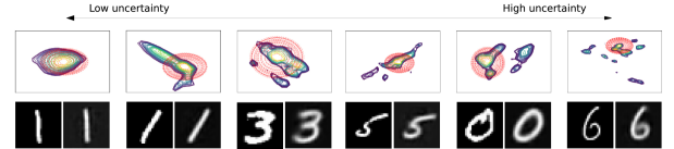
Figure 1: Uncertainty vs. posterior approximation difficulty. After the GPVAE model is trained on MNIST with 2D latent space, we evaluate the uncertainty $\textrm{Tr}\mathbb{V}({\bf f}({\bf x})|\mathcal{D})+\textrm{Tr}\mathbb{V}({\bf h}({\bf x})|\mathcal{D})$, and depict six different instances ${\bf x}$ in the order of increasing uncertainty values. Top panel shows the true posterior $p_{\bm{\theta}}({\bf z}|{\bf x})$ (contour plots) and the base encoder $\mathcal{N}({\bf b}({\bf x}),{\bf c}({\bf x})^{2})$ (red dots) superimposed (in log scale). Bottom panel contains the original inputs ${\bf x}$ (left) and reconstructed images (right). For the cases with lower uncertainty, the true posteriors are more Gaussian-like. On the other hand, the higher uncertainty cases have highly non-Gaussian true posteriors with multiple modes.

5.2 Test Inference Time

Compared to the semi-amortized methods, the inference in our GP encoder network is much faster as it is accomplished by a single feed forward pass through the encoder network. Unlike the semi-amortized approaches where one has to perform the SVI gradient adaptation at test time, in our GPVAE model, after the training stage, the posterior model is fixed, with no further adaptation required.

Table 5: (Per-batch) Test inference time (unit in milliseconds) with batch size 128. The latent dimension $\textrm{dim}({\bf z})=50$.

	MNIST	OMNIG.	CIFAR10	SVHN	CelebA
VAE	3.6	4.8	3.7	2.2	2.7
SA(1)	9.7	11.6	9.8	7.0	8.4
SA(2)	18.1	19.2	16.8	15.5	13.8
SA(4)	32.2	34.4	27.9	30.1	27.1
SA(8)	60.8	65.7	60.5	60.3	53.8
IAF(1)	4.8	5.7	5.1	3.4	4.4
IAF(2)	5.9	6.4	5.6	3.7	5.1
IAF(4)	6.2	7.0	6.3	4.7	5.7
IAF(8)	7.7	8.2	7.6	5.7	7.7
GPVAE	9.9	10.2	9.3	8.0	9.2

To verify computational speed-up over the semi-amortized approaches and others, we measure the inference. The per-batch inference times (batch size 128) on all benchmark datasets are shown in Tab. 5. To report the results, for each method and each dataset, we run inference over the entire test set batches, measure the running time, then take the per-batch average. We repeat the procedure five times and report the average. All models are run on the same machine with a single GPU (RTX 2080 Ti), Core i7 3.50GHz CPU, and 128 GB RAM.

Note that we only report test times for the latent dimension $\textrm{dim}({\bf z})=50$ since the impact of the latent dimension appears to be less significant for all models except for our GPVAE. In the GPVAE, the latent dimension can considerably affect the inference time because of the matrix operations performed per latent dimension (c.f., (13)). Hence, we consider the most complex (worst) case for our GPVAE model, $\textrm{dim}({\bf z})=50$, the highest dimension in our experimental setup. Most notably yet as expected, the semi-amortized approach (SA) suffers from the computational overhead of test time gradient updates, with the inference time significantly growing as a function of the number of increasing updates. Our GPVAE is significantly faster than the SA with more than one SVI step, albeit on par or slower than the flow-based IAF. We believe that the inference time of the GPVAE can be further improved by more effective implementations of the dimension-wise matrix operations, which remain as our future work.

5.3 Uncertainty vs. Posterior Approximation Difficulty

Another important benefit of our Bayesian treatment is that we can quantify the uncertainty in posterior approximation. Recall that our GP posterior $p({\bf f},{\bf h}|\mathcal{D})$ captures the discrepancy between the base encoder $\mathcal{N}({\bf b}({\bf x}),{\bf c}({\bf x})^{2})$ and the true posterior $p_{\bm{\theta}}({\bf x})$ via the GP noise processes ${\bf f}({\bf x})$ and ${\bf h}({\bf x})$. In particular, the variance $\mathbb{V}(f({\bf x})|\mathcal{D})$) (similarly for ${\bf h}$) at given input ${\bf x}$, can serve as a useful indicator that gauges the goodness of posterior approximation via a single Gaussian. For instance, the large posterior variance (high uncertainty) implies that the posterior approximation is difficult, suggesting the true posterior is distinct from a Gaussian (e.g., having multiple modes). On the other hand, if the variance is small (low uncertainty), one can anticipate that the true posterior might be close to a Gaussian. Fig. 1 illustrates this intuition on the MNIST dataset with 2D latent space, where the uncertainty measured by $\textrm{Tr}\mathbb{V}({\bf f}({\bf x})|\mathcal{D})+\textrm{Tr}\mathbb{V}({\bf h}({\bf x})|\mathcal{D})$ accurately aligns with the non-Gaussianity of the true posterior, closely related to the quality of reconstruction.

6 Conclusions

We have proposed a novel Gaussian process encoder model to significantly reduce the posterior approximation error of the amortized inference in VAE, while being computationally more efficient than recent semi-amortized approaches. Our Bayesian treatment that regards the discrepancy in posterior approximation as a random noise process, leads to improvements in the accuracy of inference within the fast amortized inference framework. It also offers the ability to quantify the uncertainty in variational inference, intuitively interpreted as inherent difficulty in posterior approximation. In our future work, we plan to apply GPVAE to domains with structured data, including sequences and graphs.

7 Detailed Derivations for GP Inference and Learning

We provide detailed derivations for the variational inference for GP (Sec. 3.3 in the main paper). Specifically, we show that

$$\textrm{KL}\big{(}q({\bf W},{\bf U})||p({\bf W},{\bf U}|\mathcal{D})\big{)}=\log\hat{p}_{\bm{\theta}}(\mathcal{D})-\sum_{{\bf x}\in\mathcal{D}}\textrm{ELBO}(\bm{\theta},\bm{\Lambda};{\bf x}),$$ (17)

where $\hat{p}_{\bm{\theta}}(\mathcal{D})=\mathbb{E}_{{\bf W},{\bf U}\sim\mathcal{N}({\bf 0},{\bf I})}\big{[}\prod_{{\bf x}}e^{\mathcal{L}_{\bm{\theta}}({\bf W},{\bf U};{\bf x})}\big{]}$ is the marginal data likelihood using the surrogate likelihood function $\mathcal{L}_{\bm{\theta}}({\bf W},{\bf U};{\bf x}):=\mathbb{E}_{q}\Big{[}\log\frac{p_{\bm{\theta}}({\bf x},{\bf z})}{q({\bf z}|{\bf x},{\bf W},{\bf U})}\Big{]}$, and

$$\textrm{ELBO}(\bm{\theta},\bm{\Lambda};{\bf x})=\mathbb{E}_{q({\bf z}|{\bf x})}\big{[}\log p_{\bm{\theta}}({\bf x}|{\bf z})\big{]}-\mathbb{E}_{q({\bf W},{\bf U})}[\textrm{KL}(q({\bf z}|{\bf x},{\bf W},{\bf U})||p({\bf z}))]-\frac{1}{N}\textrm{KL}(q({\bf W},{\bf U})||\mathcal{N}({\bf 0},{\bf I})).$$ (18)

Proof. Starting from the left hand side of (17),

$$\textrm{KL}\big{(}q({\bf W},{\bf U})||p({\bf W},{\bf U}|\mathcal{D})\big{)}\ =\ \mathbb{E}_{q({\bf W},{\bf U})}\Big{[}\log\frac{q({\bf W},{\bf U})}{p({\bf W},{\bf U}|\mathcal{D})}\Big{]}$$ (19)

$$\ \ =\ \mathbb{E}_{q({\bf W},{\bf U})}\Bigg{[}\log\frac{q({\bf W},{\bf U})\ \hat{p}_{\bm{\theta}}(\mathcal{D})}{\mathcal{N}({\bf W},{\bf U};{\bf 0},{\bf I})\prod_{{\bf x}\in\mathcal{D}}e^{\mathcal{L}_{\bm{\theta}}({\bf W},{\bf U};{\bf x})}}\Bigg{]}$$ (20)

$$\ \ =\ \log\hat{p}_{\bm{\theta}}(\mathcal{D})+\textrm{KL}(q({\bf W},{\bf U})||\mathcal{N}({\bf 0},{\bf I}))-\sum_{{\bf x}\in\mathcal{D}}\mathbb{E}_{q({\bf W},{\bf U})}\big{[}\mathcal{L}_{\bm{\theta}}({\bf W},{\bf U};{\bf x})\big{]}$$ (21)

$$\ \ =\ \log\hat{p}_{\bm{\theta}}(\mathcal{D})+\textrm{KL}(q({\bf W},{\bf U})||\mathcal{N}({\bf 0},{\bf I}))-\sum_{{\bf x}\in\mathcal{D}}\bigg{(}\mathbb{E}_{q({\bf z}|{\bf x})}\big{[}\log p_{\bm{\theta}}({\bf x}|{\bf z})\big{]}-\mathbb{E}_{q({\bf W},{\bf U})}\big{[}\textrm{KL}(q({\bf z}|{\bf x},{\bf W},{\bf U})||p({\bf z}))\big{]}\bigg{)}.$$ (22)

For the last equality we use the GP posterior marginalized encoder distribution,

$$q({\bf z}|{\bf x})=\iint q({\bf W},{\bf U})q({\bf z}|{\bf x},{\bf W},{\bf U})d{\bf W}d{\bf U}.$$ (23)

Arranging the last equation completes the proof.

8 Experimental Setups and Network Architectures

For all optimization, we used the Adam optimizer with batch size $128$ and learning rate $0.0005$. We run the optimization until 2000 epochs. We use the same encoder/decoder architectures for competing methods including our GPVAE, VAE, SA (semi-amortized approach), and also the base density in the flow-based models IAF and HF. The network architectures are slightly different across the datasets due to different input image dimensions. We summarize the full network architectures in Tab. 6 (MNIST and OMNIGLOT), Tab. 7 (CIFAR10 and SVHN), and Tab. 8 (CelebA).

Table 6: Encoder and decoder network architectures for MNIST and OMNIGLOT datasets. In the convolutional and transposed convolutional layers, the paddings are properly adjusted to match the input/output dimensions.

Encoder	Decoder
Input: $(28\times 28\times 1)$	Input: ${\bf z}\in$ $\mathbb{R}^{p}$ ($p\in\{10,20,50\})$
32 (4 $\times$ 4) conv.; stride 2; LeakyReLU ($0.01$)	FC. 256; ReLU
32 (4 $\times$ 4) conv.; stride 2; LeakyReLU ($0.01$)	FC. $3\cdot 3\cdot 64$; RELU
64 (4 $\times$ 4) conv.; stride 2; LeakyReLU ($0.01$)	32 (4 $\times$ 4) Transposed Conv.; stride 2; ReLU
FC. 256; LeakyReLU ($0.01$)	32 (4 $\times$ 4) Transposed Conv.; stride 2; ReLU
FC. 2 $\times p$ ($p=\textrm{dim}({\bf z})\in\{10,20,50\})$	1 (4 $\times$ 4) Transposed Conv.; stride 2

Table 7: Encoder and decoder network architectures for CIFAR10 and SVHN datasets.

Encoder	Decoder
Input: $(32\times 32\times 3)$	Input: ${\bf z}\in$ $\mathbb{R}^{p}$ ($p\in\{10,20,50\})$
32 (4 $\times$ 4) conv.; stride 2; LeakyReLU ($0.01$)	FC. 512; ReLU
32 (4 $\times$ 4) conv.; stride 2; LeakyReLU ($0.01$)	FC. $4\cdot 4\cdot 64$; RELU
64 (4 $\times$ 4) conv.; stride 2; LeakyReLU ($0.01$)	32 (4 $\times$ 4) Transposed Conv.; stride 2; ReLU
FC. 512; LeakyReLU ($0.01$)	32 (4 $\times$ 4) Transposed Conv.; stride 2; ReLU
FC. 2 $\times p$ ($p=\textrm{dim}({\bf z})\in\{10,20,50\})$	3 (4 $\times$ 4) Transposed Conv.; stride 2

Table 8: Encoder and decoder network architectures for CelebA dataset.

Encoder	Decoder
Input: $(64\times 64\times 3)$	Input: ${\bf z}\in$ $\mathbb{R}^{p}$ ($p\in\{10,20,50\})$
32 (4 $\times$ 4) conv.; stride 2; LeakyReLU ($0.01$)	FC. 512; ReLU
32 (4 $\times$ 4) conv.; stride 2; LeakyReLU ($0.01$)	FC. $4\cdot 4\cdot 64$; RELU
64 (4 $\times$ 4) conv.; stride 2; LeakyReLU ($0.01$)	64 (4 $\times$ 4) Transposed Conv.; stride 2; ReLU
64 (4 $\times$ 4) conv.; stride 2; LeakyReLU ($0.01$)	32 (4 $\times$ 4) Transposed Conv.; stride 2; ReLU
FC. 512; LeakyReLU ($0.01$)	32 (4 $\times$ 4) Transposed Conv.; stride 2; ReLU
FC. 2 $\times p$ ($p=\textrm{dim}({\bf z})\in\{10,20,50\})$	3 (4 $\times$ 4) Transposed Conv.; stride 2

9 Additional Experiments on CIFAR10

The results on the CIFAR10 dataset are reported in Tab 9.

Table 9: (CIFAR10) Test log-likelihood scores (unit in nat) estimated by the importance weighted sampling (Burda et al., 2016) with 100 samples. The figures in the parentheses next to model names indicate: the number of SVI steps in SA, the number of flows in IAF and HF, and the number of mixture components in ME and RME. The superscripts are the standard deviations. The best (on average) results are boldfaced in red. In each column, we perform the two-sided $t$-test to measure the statistical significance of the difference between the best model (red) and each competing method. We depict those with $p$-values greater than $0.01$ as boldfaced blue (little evidence of difference). So, anything plain non-colored indicates $p\leq 0.01$ (significantly different). Best viewed in color.

	$\textrm{dim}({\bf z})=10$	$\textrm{dim}({\bf z})=20$	$\textrm{dim}({\bf z})=50$
VAE	$1645.7^{4.9}$	$2089.7^{5.8}$	$2769.9^{7.1}$
SA(1)	$1645.0^{5.6}$	$2086.0^{6.2}$	$2765.0^{7.1}$
SA(2)	$1648.6^{4.8}$	$2088.2^{6.6}$	$2764.1^{7.7}$
SA(4)	$1648.5^{5.2}$	$2083.9^{8.4}$	$2766.7^{6.6}$
SA(8)	$1642.1^{5.4}$	$2086.0^{6.1}$	$2766.6^{7.5}$
IAF(1)	$1646.0^{4.9}$	$2081.1^{5.4}$	$2762.6^{7.2}$
IAF(2)	$1642.0^{4.9}$	$2084.6^{5.6}$	$2763.0^{4.3}$
IAF(4)	$1646.0^{5.1}$	$2083.2^{6.1}$	$2760.6^{7.0}$
IAF(8)	$1643.6^{4.6}$	$2087.1^{4.6}$	$2761.8^{6.9}$
HF(1)	$1644.5^{4.4}$	$2079.1^{5.5}$	$2757.9^{4.4}$
HF(2)	$1636.7^{4.9}$	$2086.0^{5.9}$	$2764.7^{4.4}$
HF(4)	$1642.1^{4.9}$	$2082.3^{7.3}$	$2763.4^{4.4}$
HF(8)	$1639.9^{5.4}$	$2084.7^{6.1}$	$2765.5^{7.2}$
ME(2)	$1643.6^{5.1}$	$2086.6^{6.8}$	$2767.9^{9.4}$
ME(3)	$1638.6^{5.8}$	$2079.8^{5.9}$	$2770.2^{7.8}$
ME(4)	$1641.8^{5.4}$	$2084.7^{6.9}$	$2763.5^{9.3}$
ME(5)	$1641.7^{5.6}$	$2080.2^{5.9}$	$2766.1^{6.3}$
RME(2)	$1652.3^{5.0}$	$2095.7^{5.8}$	$2779.6^{6.6}$
RME(3)	$1654.2^{4.9}$	$2099.1^{7.2}$	$\color[rgb]{0,0,1}{\bf 2783.0}^{6.1}$
RME(4)	$1655.0^{6.4}$	$2096.6^{5.9}$	$\color[rgb]{0,0,1}{\bf 2781.1}^{6.6}$
RME(5)	$1654.5^{4.6}$	$2098.4^{5.8}$	$\color[rgb]{0,0,1}{\bf 2782.9}^{6.4}$
GPVAE	$\color[rgb]{1,0,0}{\bf 1668.6}^{5.6}$	$\color[rgb]{1,0,0}{\bf 2113.0}^{6.7}$	$\color[rgb]{1,0,0}{\bf 2786.5}^{8.2}$

10 Importance Weighted Sampling Estimation (IWAE)

To report the test log-likelihood scores, $\log p({\bf x})$, we used the importance weighted sampling estimation (IWAE) (Burda et al., 2016). More specifically, $\textrm{IWAE}=\log\frac{1}{K}\sum_{i=1}^{K}\frac{p({\bf x},{\bf z}_{i})}{q({\bf z}_{i}|{\bf x})}$, where ${\bf z}_{1},\dots,{\bf z}_{K}$ are i.i.d. samples from $q({\bf z}|{\bf x})$. It can be shown that IWAE lower bounds $\log p({\bf x})$ and can be arbitrarily close to the target as the number of samples $K$ goes large. We used $K=100$ throughout the experiments.

11 Fully-Connected Decoder Networks

In the main paper we used the convolutional networks for both encoder and decoder models. This is a reasonable architectural choice considering that all the datasets are images. It is also widely believed that convolutional networks outperform fully connected networks for many tasks in the image domain (Krizhevsky et al., 2012; Szegedy et al., 2013; Radford et al., 2015). One can alternatively consider fully connected networks for either the encoder or the decoder, or both. Nevertheless, with the equal number of model parameters, having both convolutional encoder and decoder networks always outperformed the fully connected counterparts. In this section we empirically verify this by comparing the test likelihood performance between the two architectures. We particularly focus on comparing two architectures (convolutional vs. fully connected) for the decoder model alone, while retaining the convolutional network structure of encoders for both cases.

Using the fully connected decoder network allows us to test the recent Laplacian approximation approach (Park et al., 2019) (denoted by VLAE), which we excluded from the main paper. They use a first-order approximation solver to find the mode of the true posterior (i.e., linearizing the decoder function), and compute the Hessian of the log-posterior at the mode to define the (full) covariance matrix. This procedure is computationally feasible only for a fully connected decoder model. We conduct experiments on MNIST and OMNIGLOT datasets where the fully connected decoder network consists of two hidden layers and the hidden layer dimensions are chosen in a manner where the total number of weight parameters is roughly equal to the convolutional decoder network that we used in the main paper.

Tab. 10 summarizes the results. Among the fully connected networks, the VLAE achieves the highest performance. Instead of doing SVI gradient updates as in the SAVI method (SA), the VLAE aims to directly solve the mode of the true posterior by decoder linearization, leading to more accurate posterior refinement without suffering from the step size issue. Our GPVAE, with the fully connected decoder networks still improves the VAE’s scores, but the improvement is often less than that of the VLAE. However, when compared to the convnet decoder cases, even the conventional VAE significantly outperforms the VLAE in the ability to represent the data (markedly higher log-likelihood scores). The best VLAE’s scores are lower than even VAE’s using convolutional decoder network. Restricted network architecture in the VLAE is its main drawback.

Table 10: (Fully connected vs. convolutional decoder networks) Test log-likelihood scores (unit in nat). The figures without parentheses are the scores using the fully connected networks, whereas figures in the parentheses are the scores using the convolutional decoder networks. Both architectures have roughly equal number of weight parameters. The number of linearization steps in the VLAE is chosen among $\{1,2,4,8\}$.

	MNIST		OMNIGLOT
	$\textrm{dim}({\bf z})=10$	$\textrm{dim}({\bf z})=50$	$\textrm{dim}({\bf z})=10$	$\textrm{dim}({\bf z})=50$
VAE	563.6 (685.1)	872.6 (1185.7)	296.8 (347.0)	519.4 (801.6)
SA ($1$)	565.1 (688.1)	865.8 (1172.1)	297.6 (344.1)	489.0 (792.7)
SA ($2$)	565.3 (682.2)	868.2 (1176.3)	295.3 (349.5)	534.1 (793.1)
SA ($4$)	565.9 (683.5)	852.9 (1171.3)	294.8 (342.1)	497.8 (794.4)
SA ($8$)	564.9 (684.6)	870.9 (1183.2)	299.0 (344.8)	500.0 (799.4)
VLAE ($1$)	590.0	922.2	307.4	644.0
VLAE ($2$)	595.1	908.8	307.6	621.4
VLAE ($4$)	605.2	841.4	318.0	597.7
VLAE ($8$)	605.7	779.9	316.6	553.1
GPVAE	568.7 (693.2)	882.3 (1213.0)	302.5 (352.1)	612.5 (813.0)

We also compare the test inference times of our GPVAE model and the VLAE using the fully connected decoder networks. Note that VLAE is a semi-amortized approach that needs to perform the Laplace approximation at test time. Thus, another drawback is the computational overhead for inference, which can be demanding as the number of linearization steps increases. The per-batch inference times (batch size 128) are shown in Tab. 11. For the moderate or large linearization steps (e.g., 4 or 8), the inference takes significantly (about $2\times$ to over $3\times$) longer than that of our GPVAE (amortized method).

Table 11: (Fully connected networks as decoders) Per-batch inference time (unit in milliseconds) with batch size 128. The figures without parentheses are the times using the fully connected networks, whereas figures in the parentheses are the times using the convolutional decoder networks.

	MNIST		OMNIGLOT
	$\textrm{dim}({\bf z})=10$	$\textrm{dim}({\bf z})=50$	$\textrm{dim}({\bf z})=10$	$\textrm{dim}({\bf z})=50$
VLAE ($1$)	10.1	12.9	11.2	12.1
VLAE ($2$)	11.2	13.4	13.2	16.9
VLAE ($4$)	14.8	17.8	15.4	18.7
VLAE ($8$)	20.7	30.8	22.1	26.4
GPVAE	5.7 (5.9)	9.8 (9.9)	6.9 (6.9)	10.2 (10.2)

References

- Burda et al. (2016) Burda, Y., Grosse, R., and Salakhutdinov, R. Importance weighted autoencoders, 2016. In Proceedings of the Second International Conference on Learning Representations, ICLR.
- Cremer et al. (2018) Cremer, C., Li, X., and Duvenaud, D. Inference suboptimality in variational autoencoders. In International Conference on Machine Learning, 2018.
- Daxberger & Hernández-Lobato (2019) Daxberger, E. and Hernández-Lobato, J. M. Bayesian variational autoencoders for unsupervised out-of-distribution detection. In arXiv preprint, 2019. URL https://arxiv.org/abs/1912.05651.
- de G. Matthews et al. (2018) de G. Matthews, A. G., Hron, J., Rowland, M., Turner, R. E., and Ghahramani, Z. Gaussian process behaviour in wide deep neural networks, 2018. In International Conference on Learning Representations.
- Dezfouli & Bonilla (2015) Dezfouli, A. and Bonilla, E. V. Scalable inference for Gaussian process models with black-box likelihoods, 2015. In Advances in Neural Information Processing Systems.
- Finn et al. (2017) Finn, C., Abbeel, P., and Levine, S. Model-agnostic meta-learning for fast adaptation of deep networks. In International Conference on Machine Learning, 2017.
- Garriga-Alonso et al. (2019) Garriga-Alonso, A., Rasmussen, C. E., and Aitchison, L. Deep convolutional networks as shallow Gaussian processes, 2019. In International Conference on Learning Representations.
- Hensman et al. (2017) Hensman, J., Durrande, N., and Solin, A. Variational Fourier features for Gaussian processes. Journal of Machine Learning Research, 18:5537–5588, 2017.
- Hoffman et al. (2013) Hoffman, M. D., Blei, D. M., Wang, C., and Paisley, J. Stochastic variational inference. Journal of Machine Learning Research, 13:1303–1347, 2013.
- Huang et al. (2015) Huang, W., Zhao, D., Sun, F., Liu, H., and Chang, E. Scalable Gaussian process regression using deep neural networks, 2015. Proceedings of the Twenty-Fourth International Joint Conference on Artificial Intelligence (IJCAI).
- Kim & Pavlovic (2020) Kim, M. and Pavlovic, V. Recursive inference for variational autoencoders. Advances in Neural Information Processing Systems, 2020.
- Kim et al. (2018) Kim, Y., Wiseman, S., Millter, A. C., Sontag, D., and Rush, A. M. Semi-amortized variational autoencoders. In International Conference on Machine Learning, 2018.
- Kingma & Welling (2014) Kingma, D. P. and Welling, M. Auto-encoding variational Bayes, 2014. In Proceedings of the Second International Conference on Learning Representations, ICLR.
- Kingma et al. (2016) Kingma, D. P., Salimans, T., Jozefowicz, R., Chen, X., Sutskever, I., and Welling, M. Improving variational inference with inverse autoregressive flow, 2016. In Advances in Neural Information Processing Systems.
- Krishnan et al. (2018) Krishnan, R. G., Liang, D., and Hoffman, M. D. On the challenges of learning with inference networks on sparse high-dimensional data. In Artificial Intelligence and Statistics, 2018.
- Krizhevsky & Hinton (2009) Krizhevsky, A. and Hinton, G. Learning multiple layers of features from tiny images, 2009. Technical report, Computer Science Department, University of Toronto.
- Krizhevsky et al. (2012) Krizhevsky, A., Sutskever, I., and Hinton, G. E. Imagenet classification with deep convolutional neural networks, 2012. In Advances in Neural Information Processing Systems.
- Lake et al. (2013) Lake, B. M., Salakhutdinov, R. R., and Tenenbaum, J. One-shot learning by inverting a compositional causal process, 2013. In Advances in Neural Information Processing Systems.
- LeCun et al. (1998) LeCun, Y., Bottou, L., Bengio, Y., and Haffner, P. Gradient based learning applied to document recognition. Proceedings of the IEEE, 86(11):2278–2324, 1998.
- Lee et al. (2018) Lee, J., Bahri, Y., Novak, R., Schoenholz, S. S., Pennington, J., and Sohl-Dickstein, J. Deep neural networks as gaussian processes, 2018. In International Conference on Learning Representations.
- Liu et al. (2015) Liu, Z., Luo, P., Wang, X., and Tang, X. Deep learning face attributes in the wild. In Proceedings of International Conference on Computer Vision (ICCV), 2015.
- Lloyd et al. (2015) Lloyd, C., Gunter, T., Osborne, M. A., and Roberts, S. J. Variational inference for Gaussian process modulated Poisson processes. In International Conference on Machine Learning, 2015.
- Marino et al. (2018) Marino, J., Yisong, Y., and Mandt, S. Iterative amortized inference. In International Conference on Machine Learning, 2018.
- Neal (1996) Neal, R. M. Bayesian Learning for Neural Networks. Springer-Verlag, Berlin, Heidelberg, 1996.
- Netzer et al. (2011) Netzer, Y., Wang, T., Coates, A., Bissacco, A., Wu, B., and Ng, A. Y. Reading digits in natural images with unsupervised feature learning. 2011.
- Park et al. (2019) Park, Y., Kim, C., and Kim, G. Variational Laplace autoencoders. In International Conference on Machine Learning, 2019.
- Quiñonero-Candela & Rasmussen (2005) Quiñonero-Candela, J. and Rasmussen, C. E. A unifying view of sparse approximate Gaussian process regression. Journal of Machine Learning Research, 6:1939–1959, 2005.
- Radford et al. (2015) Radford, A., Metz, L., and Chintala, S. Unsupervised representation learning with deep convolutional generative adversarial networks. In arXiv preprint, 2015. URL https://arxiv.org/abs/1511.06434.
- Rasmussen & Williams (2006) Rasmussen, C. E. and Williams, C. K. I. Gaussian Processes for Machine Learning. The MIT Press, 2006.
- Rezende et al. (2014) Rezende, D., Mohamed, S., and Wierstra, D. Stochastic backpropagation and approximate inference in deep generative models, 2014. International Conference on Machine Learning.
- Snelson & Ghahramani (2006) Snelson, E. and Ghahramani, Z. Sparse Gaussian processes using pseudo-inputs, 2006. In Advances in Neural Information Processing Systems.
- Su et al. (2019) Su, S.-Y., Lin, S.-W., and Chen, Y.-N. Compound variational auto-encoder, 2019. IEEE International Conference on Acoustics, Speech and Signal Processing (ICASSP).
- Szegedy et al. (2013) Szegedy, C., Zaremba, W., Sutskever, I., Bruna, J., Erhan, D., Goodfellow, I., and Fergus, R. Intriguing properties of neural networks. In arXiv preprint, 2013. URL https://arxiv.org/abs/1312.6199.
- Titsias (2009) Titsias, M. K. Variational learning of inducing variables in sparse Gaussian processes, 2009. In Proceedings of the Twelfth International Conference on Artificial Intelligence and Statistics.
- Titsias et al. (2020) Titsias, M. K., Schwarz, J., de G. Matthews, A. G., Pascanu, R., and Teh, Y. W. Functional regularisation for continual learning with gaussian processes, 2020. International Conference on Learning Representations.
- Tomczak & Welling (2016) Tomczak, J. M. and Welling, M. Improving variational autoencoders using Householder flow, 2016. In Advances in Neural Information Processing Systems, Workshop on Bayesian Deep Learning.
- (37) Tran, D., Ranganath, R., and Blei, D. M. the variational gaussian process.
- Wilson et al. (2016) Wilson, A. G., Hu, Z., Salakhutdinov, R., and Xing, E. P. Deep kernel learning, 2016. AI and Statistics (AISTATS).
Supplementary Material