A new robust approach for multinomial logistic regression with complex design model

Abstract

Robust estimators and Wald-type tests are developed for the multinomial logistic regression based on $\phi$-divergence measures. The robustness of the proposed estimators and tests is proved through the study of their influence functions and it is also illustrated with two numerical examples and an extensive simulation study.

1 Introduction

Multinomial logistic regression model, also known as polytomous logistic regression model, is widely used in health and life sciences for analyzing nominal qualitative response variables and their relationship with respect to their corresponding explanatory variables or covariates. Daniels and Gatsonis (1997) used hieratical multinomial logistic regresion models to examine how the rates of cardiac procedures depend on patient-level characteristics, including age, gender and race. Dreassi (2007) also used multinomial logistic regression to detect uncommon risk factors related to oral cavity, larynx and lung cancers. Recently, Ke et al. (2016) proposed a risk prediction model using semi-varying coefficient multinomial logistic regression to assess correct prediction rates when classifying the patients with early rheumatoid arthritis. Further examples of application of these methods can be found in Blizzard and Hosmer (2007), Bull et al. (2007) and Bertens et al. (2016), among others. Although most of classical literature deals with the cases of simple random sampling scheme, the application of multinomial logistic regression model under complex survey setting (with stratification, clustering or unequal selection probabilities, for example) can be found, for example, in Binder (1983); Roberts et al. (1987); Morel (1989) and Morel and Neerchal (2012).

Most of the results mentioned above are based on (pseudo) maximum likelihood estimators (PMLEs), which are well-known to be efficient, but also non-robust. Therefore, testing procedures based on MLEs may face serious robustness problems. Castilla et al. (2018a) developed density power divergence (DPD) based robust estimators (MDPDEs) and Wald-type tests for multinomial logistic regression model under simple random sampling. This approach was extended to complex design in Castilla et al. (2020). In Castilla et al. (2018b), pseudo minimum $\phi$-divergence estimators (PM$\phi$Es), as well as new estimators for the intra-cluster correlation coefficient were developed. Estimators in the Cressie Read subfamily with tuning parameter $\lambda>0$ were shown to be an efficient alternative to classical PMLE ($\lambda=0$) for small samples sizes. However, the robustness issue was not considered. In the cited paper of Castilla et al. (2020), some simulation studies showed that Cressie Read estimators with negative tuning parameter were even more robust than MDPDEs, in terms of efficiency, for low-moderate intra-cluster correlations. However, this problem was not theoretically studied and hypothesis testing was not considered. In this paper, we prove, through the study of the influence function, the robustness of PM$\phi$Es with $-1<\lambda<0$ and we develop robust PM$\phi$Es based Wald-type tests for testing composite null hypothesis. In Section 2, we present the multinomial logistic regression model as well as the framework necessary to define the PM$\phi$Es. Based on their asymptotic distribution, robust Wald-type tests are developed in Section 3. An extensive simulation study and two numerical examples illustrate the robustness of the proposed estimators and Wald-type tests, in Section 4 and Section 5 respectively. In Appendix A, the study of the influence function of the proposed test statistics is detailed, while in Appendix B we present the proofs of the main results. Finally, in Appendix C, some extensions of the Monte Carlo simulation study are presented.

2 Multinomial logistic regression model with complex design

We consider a population $\Omega$ partitioned into $H$ strata and the data consist of $n_{h}$ clusters in stratum $h$. In the $i$-th cluster $(i=1,...,n_{h})$ within the $h$-th stratum $(h=1,...,H)$ we have observed for the $j$-th unit $(j=1,...,m_{hi})$ the values of a categorical response variable $Y$ with $d+1$ categories. Note that we assume there are $H$ strata, $n_{h}$ clusters in stratum $h$ and $m_{hi}$ units in cluster $i$ of stratum $h$. The observed responses of the $(d+1)$-dimensional variable $Y$ are denoted by the $(d+1)$-dimensional classification vector.

$$\boldsymbol{y}_{hij}=\left(y_{hij1},....,y_{hij,d+1}\right)^{T},\ h=1,...,H,i=1,...,n_{h},\text{ }j=1,...,m_{hi},$$

with $y_{hijr}$ $=1$ if the $j$-th unit selected from the $i$-th cluster of the $h$-th stratum falls in the $r$-th category and $y_{hijl}$ $=0$ for $l\neq r$. It is very common when working with dummy or qualitative explanatory variables to consider that the $k+1$ explanatory variables are common for all the individuals in the $i$-th cluster of the $h$-th stratum, being denoted as $\boldsymbol{x}_{hi}=\left(x_{hi0},x_{hi1},....,x_{hik}\right)^{T}$, with the first one, $x_{hi0}=1$, associated with the intercept.

Let us denote the sampling weight from the $i$-th cluster of the $h$-th stratum by $w_{hi}$. For each $i$, $h$ and $j$, the expectation of the $r$-th element of the random variable $\boldsymbol{Y}_{hij}=(Y_{hij1},...,Y_{hij,d+1})^{T}$, corresponding to the realization $\boldsymbol{y}_{hij}$, is determined by

$$\pi_{hir}\left(\boldsymbol{\beta}\right)=\mathrm{E}\left[Y_{hijr}|\boldsymbol{x}_{hi}\right]=\Pr\left(Y_{hijr}=1|\boldsymbol{x}_{hi}\right)=\dfrac{\exp\{\boldsymbol{x}_{hi}^{T}\boldsymbol{\beta}_{r}\}}{1+{\sum_{l=1}^{d}}\exp\{\boldsymbol{x}_{hi}^{T}\boldsymbol{\beta}_{l}\}},\quad r=1,...,d,$$ (1)

with  $\boldsymbol{\beta}_{r}=\left(\beta_{r0},\beta_{r1},...,\beta_{rk}\right)^{T}\in\mathbb{R}^{k+1}$, $r=1,...,d$ and the associated parameter space given by $\Theta=\mathbb{R}^{d(k+1)}$. It is clear that

$$\pi_{hid+1}\left(\boldsymbol{\beta}\right)=\dfrac{1}{1+{\sum_{l=1}^{d}}\exp\{\boldsymbol{x}_{hi}^{T}\boldsymbol{\beta}_{l}\}}.$$ (2)

Note that, under homogeneity, the expectation of $\boldsymbol{Y}_{hij}$ does not depends on the unit number $j$. Therefore, from now on, we will denote by

$$\widehat{\boldsymbol{Y}}_{hi}=\sum\limits_{j=1}^{m_{hi}}\boldsymbol{Y}_{hij}=\left(\sum\limits_{j=1}^{m_{hi}}Y_{hij1},...,\sum\limits_{j=1}^{m_{hi}}Y_{hij,d+1}\right)^{T}=(\widehat{Y}_{hi1},...,\widehat{Y}_{hi,d+1})^{T}$$

the random vector of counts in the $i$-th cluster of the $h$-th stratum and by $\boldsymbol{\pi}_{hi}\left(\boldsymbol{\beta}\right)$ the $(d+1)$-dimensional probability vector with the elements given in (1), $\boldsymbol{\pi}_{hi}\left(\boldsymbol{\beta}\right)=\left(\pi_{hi1}\left(\boldsymbol{\beta}\right),...,\pi_{hi,d+1}\left(\boldsymbol{\beta}\right)\right)^{T}$.

Following this notation we can define the empirical and the theoretical probability vectors of the model as

$$\widehat{\boldsymbol{p}} =\frac{1}{\tau}(w_{11}\widehat{\boldsymbol{y}}_{11}^{T},...,w_{1n_{1}}\widehat{\boldsymbol{y}}_{1n_{1}}^{T},...,w_{H1}\widehat{\boldsymbol{y}}_{H1}^{T},...,w_{Hn_{H}}\widehat{\boldsymbol{y}}_{Hn_{H}}^{T})^{T}\quad\text{and}$$ (3)

$$\boldsymbol{\pi}(\boldsymbol{\beta}) =\frac{1}{\tau}(w_{11}m_{11}\boldsymbol{\pi}_{11}^{T}(\boldsymbol{\beta}),...,w_{1n_{1}}m_{1n_{1}}\boldsymbol{\pi}_{Hn_{H}}^{T}(\boldsymbol{\beta}))^{T},$$ (4)

respectively, where $\tau=\sum\limits_{h=1}^{H}\sum\limits_{i=1}^{n_{h}}w_{hi}m_{hi}$. Probability vectors (3) and (4), both of dimension $(d+1)\sum_{h=1}^{H}n_{h}$, will play a basic role in the definition of PM$\phi$Es.

Definition 2.1

Under homogeneity assumption within the clusters and taking into account the weights $w_{hi}$, the (weighted) pseudo-maximum likelihood estimator (PMLE), $\widehat{\boldsymbol{\beta}}_{P}$, of $\boldsymbol{\beta}$ is obtained by maximizing

$$\mathcal{L}\left(\boldsymbol{\beta}\right) =\sum\limits_{h=1}^{H}\sum\limits_{i=1}^{n_{h}}w_{hi}\log\boldsymbol{\pi}_{hi}^{T}\left(\boldsymbol{\beta}\right)\widehat{\boldsymbol{y}}_{hi},$$ (5)

where $\log\boldsymbol{\pi}_{hi}^{T}\left(\boldsymbol{\beta}\right)=(\log\pi_{hi1}\left(\boldsymbol{\beta}\right),\dots,\log\pi_{hid+1}\left(\boldsymbol{\beta}\right))$.

The PMLE can be obtained as the solution of the system of equations $\boldsymbol{u}\left(\boldsymbol{\beta}\right)=\boldsymbol{0}_{d(k+1)}$, where $\boldsymbol{0}_{d(k+1)}$ is the null vector of dimension $d(k+1)$, and

$$\boldsymbol{u}\left(\boldsymbol{\beta}\right) =\sum\limits_{h=1}^{H}\sum\limits_{i=1}^{n_{h}}\boldsymbol{u}_{hi}\left(\boldsymbol{\beta}\right),\quad\boldsymbol{u}_{hi}\left(\boldsymbol{\beta}\right)=w_{hi}\boldsymbol{r}_{hi}^{\ast}\left(\boldsymbol{\beta}\right)\otimes\boldsymbol{x}_{hi},$$ (6)

where $\otimes$ is the Kronecker product and $\boldsymbol{r}_{hi}^{\ast}\left(\boldsymbol{\beta}\right)=\widehat{\boldsymbol{y}}_{hi}^{\ast}-m_{hi}\boldsymbol{\pi}_{hi}^{\ast}\left(\boldsymbol{\beta}\right)$, denoting with superscript ^∗ the vector obtained deleting the last component from the initial vector.

Remark 2.2

The distribution of  $\widehat{\boldsymbol{Y}}_{hi}$, might be unknown, as their components jointly, might be correlated. The most common assumption is to consider that  $\widehat{\boldsymbol{Y}}_{hi}$ has a multinomial sampling scheme, which means that  $\boldsymbol{Y}_{hij}$, $j=1,...,m_{hi}$ are independent random variables with covariance matrix

$$\boldsymbol{\Sigma}_{hi}=m_{hi}\boldsymbol{\Delta}(\boldsymbol{\pi}_{hi}\left(\boldsymbol{\beta}\right)),$$

with  $\boldsymbol{\Delta}(\boldsymbol{\pi}_{hi}\left(\boldsymbol{\beta}\right))=\mathrm{diag}(\boldsymbol{\pi}_{hi}\left(\boldsymbol{\beta}\right))-\boldsymbol{\pi}_{hi}\left(\boldsymbol{\beta}\right)\boldsymbol{\pi}_{hi}^{T}\left(\boldsymbol{\beta}\right)$; and since (5) is not an approximation, the term “pseudo” should be dropped. A weaker assumption is to consider that   $\widehat{\boldsymbol{Y}}_{hi}$ has a multinomial sampling scheme with a overdispersion parameter  $\nu_{hi}=1+\rho_{hi}^{2}(m_{hi}-1)$, and

$$\boldsymbol{\Sigma}_{hi}=\nu_{hi}m_{hi}\boldsymbol{\Delta}(\boldsymbol{\pi}_{hi}\left(\boldsymbol{\beta}\right)),$$

but the distribution of  $\widehat{\boldsymbol{Y}}_{hi}$ is not in principle used for the estimators. Distributions such as Dirichlet Multinomial, Random Clumped and $m$-inflated belong to this family (see Morel and Neerchal (2012); Alonso-Revenga et al. (2017) and Castilla et al. (2018c) for details). In Appendix C.1, the algorithms needed to compute these distributions in the context of PLR model with complex design are presented.

Example 2.3 (Education in Malawi)

The 2010 Malawi Demographic and Health Survey (2010 MDHS, Office and Macro (2010)) was implemented by the National Statistical Office (NSO) from June through November 2010, with a nationally representative sample of more than $27,000$ households. The sample for the 2010 MDHS was designed to provide population and health indicator estimation at the national, regional, and district levels. Let us focus on Tables 2.3.1 and 2.3.2 of the cited study, that present data on educational attainment for female and male household members age $6$ and older, divided in five wealth quintile levels, which are considered as strata. We consider here a response variable with $d+1=5$ categories: “no education”, “some primary”, “completed primary”, “some secondary”, “completed secondary or more”. For simplicity, the missing observations are not taken into account. Figure 1 shows the estimated probabilities by the PMLE of each one of the response categories for each gender. As expected, the proportion of women who have never attended any formal schooling is greater than the proportion of men and the proportion of the population that has attained education declines with its level. In the ensuing work, we will present alternative estimators to the PMLE, which are seen to provide better performance in terms of robustness.

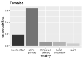
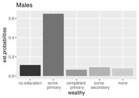
Figure 1: Estimated probabilities for wealth quintiles by gender. PMLE.

2.1 PM$\phi$Es: definition, estimation and asymptotic distribution.

Definition 2.4

Given the probability vectors (3) and (4), the family of phi-divergence measures between these probability vectors is given by

$$d_{\phi}\left(\widehat{\boldsymbol{p}},\boldsymbol{\pi}\left(\boldsymbol{\beta}\right)\right)=\frac{1}{\tau}\sum\limits_{h=1}^{H}\sum\limits_{i=1}^{n_{h}}w_{hi}m_{hi}\sum\limits_{s=1}^{d+1}\pi_{his}\left(\boldsymbol{\beta}\right)\phi\left(\frac{\widehat{y}_{his}}{m_{hi}\pi_{his}\left(\boldsymbol{\beta}\right)}\right),$$ (7)

where $\phi\in\Phi^{\ast}$ and $\Phi^{\ast}$ denotes the class of all convex functions $\phi:[0,\infty)\rightarrow\mathbb{R}\cup\{\infty\}$, such that $\phi\left(1\right)=0$, $\phi^{\prime\prime}\left(1\right)>0$ and we define $0\phi\left(0/0\right)=0$ and $0\phi\left(p/0\right)=p\lim_{u\rightarrow\infty}\phi\left(u\right)/u$.

Notice that, for $\phi(x)=x\log x-x+1$ in (7) , we have the so-called Kullback Leibler divergence. For more details about phi-divergence measures see Pardo (2005).

Let us now consider the PMLE in (5). It can be shown that it is related to the Kullback-Leibler divergence measure as follows

$$d_{KL}\left(\widehat{\boldsymbol{p}},\boldsymbol{\pi}\left(\boldsymbol{\beta}\right)\right) =K-\frac{1}{\tau}\mathcal{L}\left(\boldsymbol{\beta}\right),$$

with $K$ being a constant not dependent on $\boldsymbol{\beta}$ (Castilla et al. (2018b)). Therefore, the maximization of $\mathcal{L}\left(\boldsymbol{\beta}\right)$ is equivalent to the minimization of $d_{KL}\left(\widehat{\boldsymbol{p}},\boldsymbol{\pi}\left(\boldsymbol{\beta}\right)\right)$, i.e., PMLE is the one which minimizes the Kullback-Leibler divergence between the empirical and theoretical probability vectors, 3 and 4,

$$\widehat{\boldsymbol{\beta}}_{P}=\arg\min_{\boldsymbol{\beta\in\Theta}}d_{KL}\left(\widehat{\boldsymbol{p}},\boldsymbol{\pi}\left(\boldsymbol{\beta}\right)\right).$$ (8)

The definition of PM$\phi$E arises from the idea of generalize definition (8) to other phi-divergence measures.

Definition 2.5

We consider the multinomial logistic regression model with complex survey defined in (1). The PM$\phi$E of $\boldsymbol{\beta}$ is defined as

$$\widehat{\boldsymbol{\beta}}_{\phi,P}=\arg\min_{\boldsymbol{\beta}\in\Theta}d_{\phi}\left(\widehat{\boldsymbol{p}},\boldsymbol{\pi}\left(\boldsymbol{\beta}\right)\right).$$

Once the PM$\phi$Es are defined, it is necessary to provide the equations needed to obtain them. From equation (7), it is clear that the PM$\phi$E of $\boldsymbol{\beta}$, $\widehat{\boldsymbol{\beta}}_{\phi,P}$, is obtained by solving the system of equations $\boldsymbol{u}_{\phi}\left(\boldsymbol{\beta}\right)=\boldsymbol{0}_{d(k+1)}$, where

$$\boldsymbol{u}_{\phi}\left(\boldsymbol{\beta}\right)=\sum\limits_{h=1}^{H}\sum\limits_{i=1}^{n_{h}}\boldsymbol{u}_{\phi,hi}\left(\boldsymbol{\beta}\right),$$ (9)

with

$$\boldsymbol{u}_{\phi,hi}\left(\boldsymbol{\beta}\right) =\frac{w_{hi}m_{hi}}{\phi^{\prime\prime}(1)}\frac{\partial\boldsymbol{\pi}_{hi}^{T}(\boldsymbol{\beta})}{\partial\boldsymbol{\beta}}\boldsymbol{f}_{\phi,hi}(\tfrac{\widehat{\boldsymbol{y}}_{hi}}{m_{hi}},\boldsymbol{\beta}),\quad\frac{\partial\boldsymbol{\pi}_{hi}^{T}(\boldsymbol{\beta})}{\partial\boldsymbol{\beta}}=\left(\boldsymbol{I}_{d\times d},\boldsymbol{0}_{d\times 1}\right)\boldsymbol{\Delta}(\boldsymbol{\pi}_{hi}\left(\boldsymbol{\beta}\right))\otimes\boldsymbol{x}_{hi},$$

and

$$\boldsymbol{f}_{\phi,hi}(\tfrac{\widehat{\boldsymbol{y}}_{hi}}{m_{hi}},\boldsymbol{\beta}) =(f_{\phi,hi1}(\tfrac{\widehat{y}_{hi1}}{m_{hi}},\boldsymbol{\beta}),...,f_{\phi,hi(d+1)}(\tfrac{\widehat{y}_{hi(d+1)}}{m_{hi}},\boldsymbol{\beta}))^{T},$$

$$f_{\phi,his}(x,\boldsymbol{\beta}) =\frac{x}{\pi_{his}(\boldsymbol{\beta})}\phi^{\prime}\left(\frac{x}{\pi_{his}(\boldsymbol{\beta})}\right)-\phi\left(\frac{x}{\pi_{his}(\boldsymbol{\beta})}\right).$$

Theorem 2.6 establishes the asymptotic distribution of the PM$\phi$Es, which will be the basis of the definition of the family of Wald-type tests in Section 3. The proof of this theorem can be found in Castilla et al. (2018b).

Theorem 2.6

Let $\widehat{\boldsymbol{\beta}}_{\phi,P}$ the PM$\phi$E of parameter $\boldsymbol{\beta}$ for a multinomial logistic regression model with complex survey, $n$ the total of clusters in all the strata of the sample and $\eta_{h}^{\ast}$ an unknown proportion obtained as $\lim_{n\rightarrow\infty}\frac{n_{h}}{n}=\eta_{h}^{\ast}$, $h=1,...,H$. Then, we have

$$\sqrt{n}(\widehat{\boldsymbol{\beta}}_{\phi,P}-\boldsymbol{\beta}^{0})\overset{\mathcal{L}}{\underset{n\mathcal{\rightarrow}\infty}{\longrightarrow}}\mathcal{N}\left(\boldsymbol{0}_{d(k+1)},\mathbf{J}^{-1}\left(\boldsymbol{\beta}^{0}\right)\mathbf{G}\left(\boldsymbol{\beta}^{0}\right)\mathbf{J}^{-1}\left(\boldsymbol{\beta}^{0}\right)\right),$$ (10)

where $\boldsymbol{\beta}^{0}$ is the true parameter value and

$$\mathbf{J}\left(\boldsymbol{\beta}\right) =\lim_{n\rightarrow\infty}\mathbf{J}_{n}\left(\boldsymbol{\beta}\right)=\sum\limits_{h=1}^{H}\eta_{h}^{\ast}\lim_{n_{h}\rightarrow\infty}\mathbf{J}_{n_{h}}^{(h)}\left(\boldsymbol{\beta}\right),$$

$$\mathbf{G}\left(\boldsymbol{\beta}\right) =\lim_{n\rightarrow\infty}\mathbf{G}_{n}\left(\boldsymbol{\beta}\right)=\sum\limits_{h=1}^{H}\eta_{h}^{\ast}\lim_{n_{h}\rightarrow\infty}\mathbf{G}_{n_{h}}^{(h)}\left(\boldsymbol{\beta}\right),$$

with

$$\mathbf{J}_{n}\left(\boldsymbol{\beta}\right) =\frac{1}{n}\sum\limits_{h=1}^{H}\sum\limits_{i=1}^{n_{h}}w_{hi}m_{hi}\boldsymbol{\Delta}(\boldsymbol{\pi}_{hi}^{\ast}\left(\boldsymbol{\beta}\right))\otimes\boldsymbol{x}_{hi}\boldsymbol{x}_{hi}^{T},$$

$$\mathbf{J}_{n_{h}}^{(h)}\left(\boldsymbol{\beta}\right) =\frac{1}{n_{h}}\sum\limits_{i=1}^{n_{h}}w_{hi}m_{hi}\boldsymbol{\Delta}(\boldsymbol{\pi}_{hi}^{\ast}\left(\boldsymbol{\beta}\right))\otimes\boldsymbol{x}_{hi}\boldsymbol{x}_{hi}^{T},$$

$$\mathbf{G}_{n}\left(\boldsymbol{\beta}\right) =\frac{1}{n}\sum\limits_{h=1}^{H}\sum\limits_{i=1}^{n_{h}}\mathbf{V}[\boldsymbol{U}_{hi}\left(\boldsymbol{\beta}\right)],$$

$$\mathbf{G}_{n_{h}}^{(h)}\left(\boldsymbol{\beta}\right) =\frac{1}{n_{h}}\sum\limits_{i=1}^{n_{h}}\mathbf{V}[\boldsymbol{U}_{hi}\left(\boldsymbol{\beta}\right)],\text{\quad}\mathbf{V}[\boldsymbol{U}_{hi}\left(\boldsymbol{\beta}\right)]=w_{hi}^{2}\mathbf{V}[\widehat{\boldsymbol{Y}}_{hi}^{\ast}]\otimes\boldsymbol{x}_{hi}\boldsymbol{x}_{hi}^{T},$$

$\mathbf{J}\left(\boldsymbol{\beta}\right)$ is the Fisher information matrix, $\mathbf{V}[\boldsymbol{\cdot}]$ denotes the variance-covariance matrix of a random vector and $\boldsymbol{U}_{hi}\left(\boldsymbol{\beta}\right)$ is the random variable generator of $\boldsymbol{u}_{hi}\left(\boldsymbol{\beta}\right)$, given by (6).

Remark 2.7

Matrices $\mathbf{J}(\boldsymbol{\beta}^{0})$ and $\mathbf{G}(\boldsymbol{\beta}^{0})$ of Theorem 2.6 can be consistently estimated as

$$\widehat{\mathbf{J}}_{n}(\widehat{\boldsymbol{\beta}}_{\phi,P}) =\frac{1}{n}\sum\limits_{h=1}^{H}\sum\limits_{i=1}^{n_{h}}w_{hi}m_{hi}\boldsymbol{\Delta}(\boldsymbol{\pi}_{hi}^{\ast}(\widehat{\boldsymbol{\beta}}_{\phi,P}))\otimes\boldsymbol{x}_{hi}\boldsymbol{x}_{hi}^{T}$$

$$\widehat{\mathbf{G}}_{n}(\widehat{\boldsymbol{\beta}}_{\phi,P}) =\frac{1}{n}\sum\limits_{h=1}^{H}\sum\limits_{i=1}^{n_{h}}\left(\boldsymbol{u}_{hi}(\widehat{\boldsymbol{\beta}}_{\phi,P})-\frac{1}{n}\boldsymbol{u}(\widehat{\boldsymbol{\beta}}_{\phi,P})\right)\left(\boldsymbol{u}_{hi}(\widehat{\boldsymbol{\beta}}_{\phi,P})-\frac{1}{n}\boldsymbol{u}(\widehat{\boldsymbol{\beta}}_{\phi,P})\right)^{T}.$$

An important family of phi-divergence measures is obtained by restricting $\phi$ from the family of convex functions $\Phi^{*}$ to the Cressie-Read subfamily, that is to say, $\phi$ is of the following form:

$$\phi_{\lambda}(x)=\left\{\begin{array}[]{ll}\frac{1}{\lambda(1+\lambda)}\left[x^{\lambda+1}-x-\lambda(x-1)\right],&\lambda\in\mathbb{R}-\{-1,0\}\\ \lim_{\upsilon\rightarrow\lambda}\frac{1}{\upsilon(1+\upsilon)}\left[x^{\upsilon+1}-x-\upsilon(x-1)\right],&\lambda\in\{-1,0\}\end{array}\right..$$

For the Cressie-Read subfamily, it is established that for $\lambda\neq-1$,

$$\boldsymbol{u}_{\phi_{\lambda}}\left(\boldsymbol{\beta}\right)=\sum\nolimits_{h=1}^{H}\sum\nolimits_{i=1}^{n_{i}}\boldsymbol{u}_{\phi_{\lambda},hi}\left(\boldsymbol{\beta}\right),$$

where

$$\boldsymbol{u}_{\phi_{\lambda},hi}\left(\boldsymbol{\beta}\right)=\frac{w_{hi}}{(\lambda+1)m_{hi}^{\lambda}}\boldsymbol{\Delta}^{*}(\boldsymbol{\pi}_{hi}(\boldsymbol{\beta}))\mathrm{diag}^{-(\lambda+1)}(\boldsymbol{\pi}_{hi}(\boldsymbol{\beta}))\widehat{\boldsymbol{y}}_{hi}^{\lambda+1}\otimes\boldsymbol{x}_{hi},$$ (11)

where

$$\boldsymbol{\Delta}^{*}(\boldsymbol{\pi}_{hi}(\boldsymbol{\beta}))=(\boldsymbol{I}_{d},\boldsymbol{0}_{d})\boldsymbol{\Delta}(\boldsymbol{\pi}_{hi}(\boldsymbol{\beta})).$$

We can observe that for $\lambda=0$, we have

$$\phi_{\lambda=0}(x)=\lim_{\upsilon\rightarrow 0}\frac{1}{\upsilon(1+\upsilon)}\left[x^{\upsilon+1}-x-\upsilon(x-1)\right]=x\log x-x+1,$$

and the associated phi-divergence, coincides with the Kullback divergence. Therefore, the PM$\phi$E of $\boldsymbol{\beta}$ based on $\phi_{\lambda}(x)$ contains as special case the PMLE and $\boldsymbol{u}_{hi}\left(\boldsymbol{\beta}\right)$ given in (6) matches $\boldsymbol{u}_{\phi,hi}\left(\boldsymbol{\beta}\right)$ given in (11). Other important divergences are obtained inside this family: for $\lambda=1$ the chi-square divergence, for $\lambda=2/3$ the Cressie-Read divergence and for $\lambda=-0.5$ the Hellinger distance. Note that the Hellinger distance is well-known in statistical theory for its robustness (Lindsay et al. (1994)). The robustness of (Cressie-Read) PM$\phi$Es for $-1<\lambda<0$ is proved, through the study of their influence function, in Appendix A.

Remark 2.8

Along this paper, we are referring to the case of complex sample survey. These all procedures can be easily simplified to the case of simple sample survey by considering a single stratum and considering “observations” instead of clusters. Some work has been done within the phi-divergence measures and multinomial logistic regression (see Gupta et al. (2008); Martín and Pardo (2014)) but, to the best of our knowledge, the robustness issue was not previously considered. In Section 5.2, an example is provided to illustrate the application of the proposed methods also in this context.

3 Robust Wald-type tests

In the last years, it has been very common in the statistical literature to consider Wald-type tests based on the minimum distance estimators instead of the MLE. The resulting tests have an excellent behaviour in relation to the robustness with a non-significant loss of efficiency, see for instance, Basu et al. (2017, 2018). In this section, we will introduce Wald-type test statistics based on the PM$\phi$Es as a generalization of the classical Wald test based on PMLE. As it happened with PM$\phi$Es, the robustness of these proposed Wald-type tests can be proved for $-1<\lambda<0$ (see Appendix A).

In this context, we are interested in testing

$$H_{0}:\boldsymbol{M}^{T}\boldsymbol{\beta}=\boldsymbol{m}\quad\text{against}\quad\boldsymbol{M}^{T}\boldsymbol{\beta}\neq\boldsymbol{m},$$ (12)

where $\boldsymbol{M}$ is $d(k+1)\times r$ full rank matrix with $r\leq d(k+1)$ and $\boldsymbol{m}$ an $r$-vector.

Definition 3.1

Let $\widehat{\boldsymbol{\beta}}_{\phi,P}$ the PM$\phi$E of $\boldsymbol{\beta}$ and denote

$$\widehat{\mathbf{V}}_{n}(\widehat{\boldsymbol{\beta}}_{\phi,P})=\widehat{\mathbf{J}}_{n}^{-1}(\widehat{\boldsymbol{\beta}}_{\phi,P})\widehat{\mathbf{G}}_{n}(\widehat{\boldsymbol{\beta}}_{\phi,P})\widehat{\mathbf{J}}_{n}^{-1}(\widehat{\boldsymbol{\beta}}_{\phi,P}).$$

Then, the family of Wald-type test statistics for testing the null hypothesis given in (12) is defined as

$$W_{n}(\widehat{\boldsymbol{\beta}}_{\phi,P})=n\left(\boldsymbol{M}^{T}\widehat{\boldsymbol{\beta}}_{\phi,P}-\boldsymbol{m}\right)^{T}\left[\boldsymbol{M}^{T}\mathbf{V}_{n}(\widehat{\boldsymbol{\beta}}_{\phi,P})\boldsymbol{M}\right]^{-1}\left(\boldsymbol{M}^{T}\widehat{\boldsymbol{\beta}}_{\phi,P}-\boldsymbol{m}\right).$$ (13)

Theorem 3.2

The asymptotic distribution of the Wald-type test statistics, $W_{n}(\widehat{\boldsymbol{\beta}}_{\phi,P})$, under the null hypothesis in (12), is a chi-square distribution with $r$ degrees of freedom.

Corollary 3.3

Based on Theorem 3.2, the null hypothesis in (12) will be rejected if

$$W_{n}(\widehat{\boldsymbol{\beta}}_{\phi,P})>\chi^{2}_{r,\alpha}$$ (14)

being $\chi^{2}_{r,\alpha}$ the upper $\alpha$-th quantile of $\chi^{2}_{r}$.

The following theorem may be used to approximate the power function for the Wald- type test statistics given in (14).

Theorem 3.4

Let $\boldsymbol{\beta}^{0}$ be the true value of the parameter and let us denote

$$\ell^{\ast}\left(\boldsymbol{\beta}_{1}\mathbf{,}\boldsymbol{\beta}_{2}\right)=\left(\boldsymbol{M}^{T}\boldsymbol{\beta}_{1}-\boldsymbol{m}\right)^{T}\left(\boldsymbol{M}^{T}\mathbf{V}\left(\boldsymbol{\beta}_{2}\right)\boldsymbol{M}\right)^{-1}\left(\boldsymbol{M}^{T}\boldsymbol{\beta}_{1}-\boldsymbol{m}\right).$$

Then it holds

$$\sqrt{n}\left(\ell^{\ast}(\widehat{\boldsymbol{\beta}}_{\phi,P},\boldsymbol{\beta^{0}})-\ell^{\ast}\left(\boldsymbol{\beta^{0},\beta^{0}}\right)\right)\underset{n\rightarrow\infty}{\overset{L}{\longrightarrow}}\mathcal{N}(0,\sigma_{W}^{2}\left(\boldsymbol{\beta^{0}}\right)),$$

where

$$\sigma_{W}^{2}\left(\boldsymbol{\beta^{0}}\right)=4\left(\boldsymbol{M}^{T}\boldsymbol{\beta}^{0}-\boldsymbol{m}\right)^{T}\left(\boldsymbol{M}^{T}\mathbf{V}\left(\boldsymbol{\beta}^{0}\right)\boldsymbol{M}\right)^{-1}\left(\boldsymbol{M}^{T}\boldsymbol{\beta}^{0}-\boldsymbol{m}\right).$$

Theorem 3.5

Let $\boldsymbol{\beta}^{0}\in\Theta$, with $\boldsymbol{M}^{T}\boldsymbol{\beta}^{0}\neq\boldsymbol{m}$, be the true value of the parameter such that $\widehat{\boldsymbol{\beta}}_{\phi,P}\underset{n\rightarrow\infty}{\overset{P}{\longrightarrow}}\boldsymbol{\beta}^{0}$. The power function of the Wald-type test given in (14), is given by

$$\Pi_{W_{n}(\widehat{\boldsymbol{\beta}}_{\phi,P})}\left(\boldsymbol{\beta}^{0}\right)=1-\Phi_{n}\left(\frac{1}{\sigma_{W}\left(\boldsymbol{\beta}^{0}\right)}\left(\frac{\chi_{r,\alpha}^{2}}{\sqrt{n}}-\sqrt{n}\ \ell^{\ast}(\widehat{\boldsymbol{\beta}}_{\phi,P},\boldsymbol{\beta^{0}})\right)\right)$$ (15)

where $\Phi_{n}\left(x\right)$ uniformly tends to the standard normal distribution as $n\rightarrow\infty$.

Corollary 3.6

It is clear that

$$\lim_{n\rightarrow\infty}\Pi_{W_{n}(\widehat{\boldsymbol{\beta}}_{\phi,P})}\left(\boldsymbol{\beta}^{0}\right)=1$$

for all $\alpha\in\left(0,1\right)$. Therefore, the Wald-type tests are consistent in the sense of Fraser.

Remark 3.7

Theorem 3.5 can be applied in the sense of getting the necessary sample size in order to get that the Wald-type tests have a determinate fix power, i.e., $\Pi_{W_{n}(\widehat{\boldsymbol{\beta}}_{\phi,P})}\left(\boldsymbol{\beta}^{0}\right)\equiv\pi^{0}$ and size $\alpha$. The necessary sample size is given by

$$n=\left[\frac{A+B+\sqrt{A(A+2B)}}{2\ell^{\ast}\left(\boldsymbol{\beta}^{0},\boldsymbol{\beta}^{0}\right)^{2}}\right]+1,$$

where $\left[x\right]$ denotes the largest integer less than or equal to $x$, $A=\sigma_{W}^{2}\left(\boldsymbol{\beta}^{0}\right)\left(\Phi^{-1}(1-\pi^{0})\right)^{2}$ and $B=2\ell^{\ast}\left(\boldsymbol{\beta}^{0},\boldsymbol{\beta}^{0}\right)\chi_{r,\alpha}^{2}$.

We may also find approximations of the power function of the Wald-type tests given in (13) at an alternative hypothesis close to the null hypothesis. Let $\boldsymbol{\beta}_{n}\in\Theta-\Theta_{0}$ be a given alternative, and let $\boldsymbol{\beta}_{0}\in\Theta_{0}$ (null hypothesis) the element closest to $\boldsymbol{\beta}_{n}$ in terms of the Euclidean distance. We may introduce contiguous alternative hypotheses by considering a fixed $\boldsymbol{d}\in\mathbb{R}^{d(k+1)}$ and to permit $\boldsymbol{\beta}_{n}$ moving towards $\boldsymbol{\beta}_{0}$ as $n$ increases through the relation

$$H_{1,n}:\boldsymbol{\beta}_{n}=\boldsymbol{\beta}_{0}+n^{-1/2}\boldsymbol{d}.$$ (16)

Let us now relax the condition $\boldsymbol{M}^{T}\boldsymbol{\beta}_{0}=\boldsymbol{m}$ defining the null hypothesis. Let $\boldsymbol{\delta}\in\mathbb{R}^{r}$ and consider the following sequence, $\boldsymbol{\beta}_{n}$, of parameters moving towards $\boldsymbol{\beta}_{0}$ according to

$$H_{1,n}^{\ast}:\boldsymbol{M}^{T}\boldsymbol{\beta}_{n}-\boldsymbol{m}=n^{-1/2}\boldsymbol{\delta}.$$ (17)

Theorem 3.8

The asymptotic distribution of  $W_{n}(\widehat{\boldsymbol{\beta}}_{\phi,P})$ is given by:

• Under $H_{1,n}$, $W_{n}(\widehat{\boldsymbol{\beta}}_{\phi,P})\underset{n\rightarrow\infty}{\overset{\mathcal{L}}{\longrightarrow}}\chi_{r}^{2}\left(\Delta\right)$, where $\Delta$ is the parameter of non-centrality given by

  $$\Delta=\boldsymbol{d}^{T}\boldsymbol{M}\left[\boldsymbol{M}^{T}\mathbf{V}(\boldsymbol{\beta}_{0})\boldsymbol{M}\right]^{-1}\boldsymbol{M}^{T}\boldsymbol{d},$$

• Under $H^{*}_{1,n}$, $W_{n}(\widehat{\boldsymbol{\beta}}_{\phi,P})\underset{n\rightarrow\infty}{\overset{\mathcal{L}}{\longrightarrow}}\chi_{r}^{2}\left(\Delta^{*}\right)$, where $\Delta^{*}$ is the parameter of non-centrality given by

  $$\Delta^{*}=\boldsymbol{d}^{T}\boldsymbol{M}\left[\boldsymbol{M}^{T}\mathbf{V}(\boldsymbol{\beta}_{0})\boldsymbol{M}\right]^{-1}\boldsymbol{M}^{T}\boldsymbol{d}.$$

Proofs of the results given in this section can be found in Appendix B.

4 Monte Carlo Simulation Study

In this section, we develop a simulation study in order to illustrate the robustness of the proposed estimators and Wald-type tests based on them. Following the simulation studies proposed in Castilla et al. (2018a) and Castilla et al. (2020), we consider $H=4$ strata with $n_{h}$ clusters of the same size $m$, with $m=20$ and $n_{h}\in\{10,20,..,60\}$ for $h=1,\dots,H$. We consider $d+1=3$ categories on the response variable, depending on $k=2$ explanatory variables. The response variable $\widehat{\boldsymbol{Y}}_{hi}$, described as

$$\boldsymbol{E}[\widehat{\boldsymbol{Y}}_{hi}] =m\boldsymbol{\pi}_{hi}\left(\boldsymbol{\beta}^{0}\right)\quad\text{and}\quad\boldsymbol{V}[\widehat{\boldsymbol{Y}}_{hi}]=\nu_{m}m\boldsymbol{\Delta}(\boldsymbol{\pi}_{hi}\left(\boldsymbol{\beta}^{0}\right)),$$

$$\nu_{m} =1+\rho^{2}(m-1),\quad i=1,\dots,n_{h},\ h=1,\dots,H,$$

is considered to follow the m-Inflated multinomial distribution (see Remark 2.2), with parameters $\rho^{2}=0.5$ and $\boldsymbol{\pi}_{hi}\left(\boldsymbol{\beta}^{0}\right)$, given by the logistic relationship (1) with

$$\boldsymbol{\beta}^{0}=(\beta_{01},\beta_{11},\beta_{21},\beta_{02},\beta_{12},\beta_{22})^{T}=(0,-0.9,0.1,0.6,-1.2,0.8)^{T}$$

and $\boldsymbol{x}_{hi}\overset{iid}{\sim}\mathcal{N}(\boldsymbol{0},\boldsymbol{I})$ for all $i=1,\ldots,n_{h}$, $h=1,\dots,H$. In order to study the robustness issue, these simulations are repeated under contaminated data having $10\%$ outliers. These outliers are generated by permuting the elements of the outcome variable, such that categories 1, 2, 3 are classified as categories 3, 1, 2 for the outlying observations. Note that this view of considering outliers as classification errors in the PLR model is, in fact, in line with the general literature on robust analysis of categorical data (Johnson (1985); Croux and Haesbroeck (2003)) and is covered with the theory developed in Appendix A, where our “outlier producing measure” indeed provides classification error if the outlier point yields its mass in a wrong category (see Castilla et al. (2020) for more details).

In this scenario, the root of mean square error (RMSE) for the Cressie-Read PM$\phi$Es of $\boldsymbol{\beta}$ with $\lambda\in\{-0.5,-0.3,0,2/3\}$ is studied, both for the contaminated and not-contaminated cases (see top of Figure 2). To compute the accuracy in terms of contrast, we consider the testing problem

$$H_{0}:\beta_{11}=-0.9\quad\text{vs.}\quad H_{1}:\beta_{11}\neq-0.9.$$

For computing the empirical test level, we measured the proportion of Wald-type test statistics ex- ceeding the corresponding chi-square critical value. The simulated test powers were also obtained under $H_{1}$ in in a similar manner (here we consider $\beta_{11}=-1.5$). We used a nominal level of $0.05$. Both levels and powers are presented in the middle and bottom of Figure 2.

It is observed that PMLE ($\lambda=0$) presents the best behavior in terms of efficiency for the non-contaminated setting. In addition, PM$\phi$E with $\lambda=0.66$ presents a RMSE lower than PM$\phi$E with negative values of $\lambda$. On the other hand, when it is considered the contaminated setting, PM$\phi$E with $\lambda=-0.3$ presents a better behavior as it can be seen for high values of $n_{h}$. The other negative value considered for PM$\phi$E improves clearly the RMSE regarding to $\lambda=0.66$, again, for high values of $n_{h}$. However, the greatest difference is observed when studying empirical levels and powers. Although PMLE remains the best estimator for testing in a pure scenario, for the contaminated setting, better empirical levels are observed for negative values of the tuning parameter $\lambda$, in particular, for $\lambda=-0.5$. In terms of powers, negative values of $\lambda$ present better behavior in both settings, non-contaminated and contaminated. Positive values of $\lambda$ are presented as a good alternative only in terms of efficiency for small sample sizes, in concordance with Castilla et al. (2018b). Other alternative scenarios are considered in Appendix C.

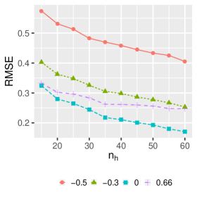
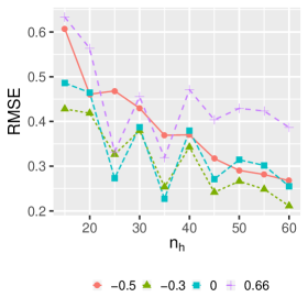
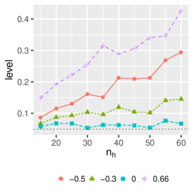
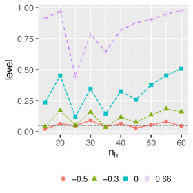
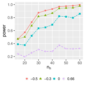
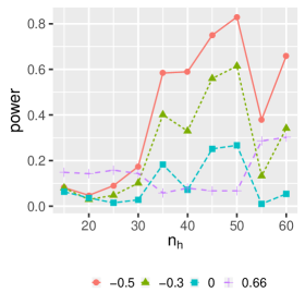
Figure 2: RMSEs (top), emprirical levels (middle) and empirical powers (bottom). Non-contaminated and contaminated settings (left and right, respectively). m-Inflated distribution.

5 Numerical Examples

5.1 Education in Malawi (continuation)

Let us continue with the 2010 MDHS presented in Example 2.3. As pointed out there, the 2010 MDHS presents data on educational attainment for female and male by its wealth quintile level. In this section, we make a comparison of the behaviour between different PM$\phi$Es, when estimating the probabilities of the response categories. For this purpose, and after estimating the PM$\phi$Es in a grid of tuning parameters $\lambda\in\{-0.5,0.7\}$ in the Cressie-Read subfamily, we measure a pondered standardized mean absolute error (SMAE) of the estimated probabilities against the observed probabilities. This is done by distinguishing the strata (wealth quintiles), the clusters (female and male) and jointly, as it can be seen in Figure 3. The lowest SMAEs are obtained for negative values of $\lambda$. Then, they seem to offer a better behavior than the classical PMLE.

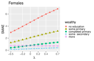
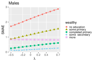
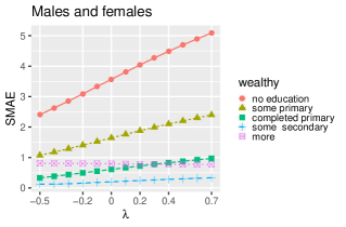
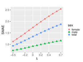
Figure 3: Education in Malawi: estimated SMAEs for different values of the tuning parameter.

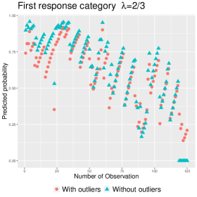
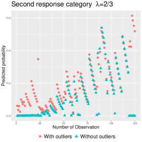
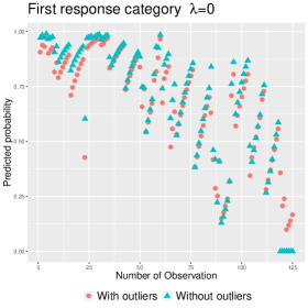
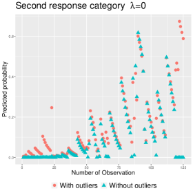
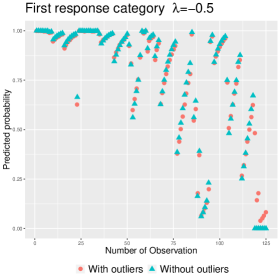
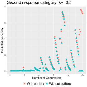
Figure 4: Mamography example: predicted category probabilities of the response variable for the MLE ($\lambda=0$) and M$\phi$Es with $\lambda=2/3$ and $\lambda=-0.5$.

5.2 Mammography experience data

As noted in Remark 2.8, multinomial logistic regression model under complex sample design is an extension of the classical one, evaluated under a simple sample design. Therefore, the tools developed in this paper, can be also applied to these cases, in which the data design may be much simpler. In this section, we study the Mammography experience data, a subset of a study by the University of Massachusetts Medical School, introduced in Hosmer and Lemeshow (2000) and recently studied by Martín (2015) and Castilla et al. (2018a). This study, which assess factors associated with women’s knowledge, attitude and behavior towards mammography, involves $412$ individuals, grouped in $125$ distinct covariates values (which, somehow correspond to the “clusters” in a more complex survey) and $8$ explanatory variables, detailed in the cited bibliography. The response variable ME (Mammography experience) is a categorical factor with three levels: “Never”, “Within a Year” and “Over a Year”. As suggested by Martín (2015), the groups of observations associated with covariate values $\boldsymbol{x}_{i}$ for $i\in\{1,3,17,35,75,81,102\}$ can be treated as outliers. So this data set is a perfect candidate to show the robustness performance of the proposed estimators.

We compute the minimum $\phi$-divergence estimators (M$\phi$Es) of $\boldsymbol{\beta}$ for $\lambda\in\{-0.5,0,2/3\}$, for the full dataset and also for the outliers deleted dataset. Moreover, we plot the corresponding (estimated) category probabilities for each available distinct covariate values. The left panel of Figure 4 presents these category probabilities for the first category, while the right panel presents these category probabilities for the second category. Results clearly indicate the significant variation of the MLE and M$\phi$E with $\lambda=2/3$ in the presence or absence of the outliers (red circles and blue triangles, respectively). However, the M$\phi$E with $\lambda=-0.5$ is shown to be much more stable, which is in concordance with its theoretical robustness.

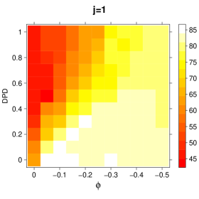
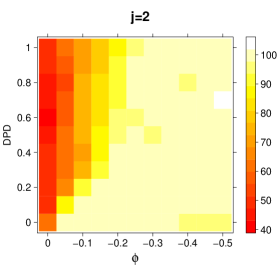
Figure 5: Mamography example: comparation of M$\phi$Es and MDPDEs.

In Castilla et al. (2018a) this dataset was also analyzed in order to illustrate the robustness of other family of estimators, those based on DPD divergences, the MDPDEs. This family is also parametrized by a tuning parameter, let say, $\lambda^{*}\geq 0$, and contains the MLE as a particular case for $\lambda^{*}=0$. The question that could arise here is the point on using PM$\phi$Es instead of MDPDEs. In this regard, the efficiency of both family of estimators is compared in the following way: for each pair of tuning parameters $(\lambda,\lambda^{*})$ in a grid on $[-0.5,0]\times[0,1]$, the M$\phi$Es and MDPDEs are computed and the estimated probabilities for each of the categories of the response variable are obtained for each of the $I=125$ observations. Then, we count the number of times, in these $125$ observations, that the M$\phi$E presents a lower error (the estimated probability is closer to the observed probability) than the MDPDE. The higher this value is, the better is the M$\phi$E with respect to the MDPDE. If the value is under $[I/2]=63$, then the MDPDE is preferable. These results are illustrated in the two heat plots (for the first and second category, the third is omitted since it is similar) on Figure 5. We can observe how M$\phi$Es with a low value of $\lambda$ improves any MDPDE, while MDPDEs with a large value of $\lambda^{*}$ only improves PM$\phi$Es with tuning parameters near to $0$. The efficiency of the MLE is not comparable to any other option.

Now, we want to evaluate the robustness of the proposed Wald-type tests. We consider the problem of testing

$$H_{0}:\beta_{SYMPT_{12}}=0,$$

$$H_{0}:\beta_{SYMPT_{11}}=\beta_{SYMPT_{21}},$$

for the variable SYMPT (“You do not need a mammogram unless you develop symptoms: 1, strongly agree; 2, agree; 3, disagree; 4, strongly disagree). The p-values obtained based on the proposed test are plotted over $\lambda$ in Figure 6 for both the full and the outlier deleted data. Clearly, the test decision at the significance level $\alpha=0.1$ changes completely in the presence of outliers for $\lambda$ near to $0$.

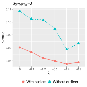
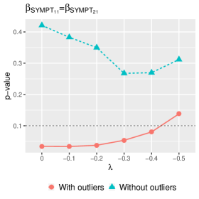
Figure 6: Mamography example: p-values of the proposed M$\phi$Es based Wald-type tests.

6 Concluding Remarks and Future Work

In this paper, we present robust estimators (PM$\phi$E) and Wald-type tests based on them for the multinomial logistic regression under complex survey, by means of $\phi$-divergence measures. In particular, we focus our study in the Cressie-Read subfamily of divergences, which are modelized by a tuning parameter $\lambda$. It is theoretically proved and empirically illustrated how PM$\phi$Es and Wald-type tests with $-1<\lambda<0$ are more robust than the classical PMLE and Wald-test, presenting an interesting alternative to them. We believe that this method may be of special interest for analyzing demographic and health surveys, such as the one presented in Section 5.2, as well as overall complex surveys for developing countries.

One of the problems that arises here is, given any data set, the choice of the tuning parameter $\lambda$. Robustness is usually accompanied with a loss of efficiency and other factors, such as sample size, can be also determinant in this decision. One possible way to make this choice is as follows: in a grid of possible tuning parameters, apply a measure of discrepancy to the data. Then, the tuning parameter that leads to the minimum discrepancy-statistic can be chosen as the “optimal” one. This is, somehow, the idea followed in the examples (see Figure 3 and 5). Another alternative is the one proposed by Warwick and Jones (2005), which consists on minimizing the estimated mean square error, computed as the sum of the squared (estimated) bias and variance. One of the main drawbacks of this method is the fact that it depends on a pilot estimator to estimate the bias. This problem was also highlighted recently in Basak et al. (2020), where an “iterative Warwick and Jones algorithm” (IJW algorithm) is proposed. Application of these methods and a development of new ones will be a challenging and interesting problem for further consideration.

Acknowledgments: This research is partially supported by Grant PGC2018-095194-B-I00, Grant FPU16/03104 and Grant BES-2016- 076669 from Ministerio de Ciencia, Innovación y Universidades and Ministerio de Economía, Industria y Competitividad (Spain). E. Castilla is member of the Instituto de Matemática Interdisciplinar, Complutense University of Madrid.

Appendix A Study of the Robustness of the proposed estimators and Wald-type tests

An important concept in robustness theory is the influence function (Hampel et al. (1986)). For any estimator defined in terms of a statistical functional $\boldsymbol{U}(F)$ from the true distribution $F$, its influence function (IF) is defined as

$${IF}(t,\boldsymbol{U},F)=\lim_{\varepsilon\downarrow 0}\frac{\boldsymbol{U}(F_{\varepsilon})-\boldsymbol{U}(F)}{\varepsilon}=\left.\frac{\partial\boldsymbol{U}(F_{\varepsilon})}{\partial\varepsilon}\right|_{\varepsilon=0^{+}},$$ (18)

where $F_{\varepsilon}=(1-\varepsilon)F+\varepsilon\Delta_{t}$, with $\varepsilon$ being the contamination proportion and $\Delta_{t}$ being the degenerate distribution at the contamination point $t$. Thus, the (first-order) IF, as a function of $t$, measures the standardized asymptotic bias (in its first-order approximation) caused by the infinitesimal contamination at the point $t$. The maximum of this IF over $t$ indicates the extent of bias due to contamination and so smaller its value, the more robust the estimator is.

The classical theory deals with the case of independent and identically distributed (iid) observations (Lindsay et al. (1994)). However, the present set-up of complex survey is not as simple as the iid set-up; in fact the observations within a cluster of a stratum are iid but the observations in different cluster and stratum are independent non-homogeneous. So we need to modify the definition of the influence function accordingly. Recently, Ghosh and Basu (2013, 2015, 2018) have discussed the extended definition of the influence function for the independent but non-homogeneous observations; however, all these works have been developed for DPD-based estimators. Here, we will extend their definition for the case of multinomial logistic regression and PM$\phi$DEs.

We first need to define the statistical functional $\boldsymbol{U}_{\phi}(\boldsymbol{\beta})$ corresponding to the PM$\phi$Es as the minimizer of the phi-divergence between the true and the model densities. This is defined as the minimizer of

$$\boldsymbol{H}_{\phi}(\boldsymbol{\beta})=\frac{1}{\tau}\sum\limits_{h=1}^{H}\sum\limits_{i=1}^{n_{h}}w_{hi}m_{hi}\sum\limits_{s=1}^{d+1}\pi_{his}\left(\boldsymbol{\beta}\right)\phi\left(\frac{g_{his}}{\pi_{his}\left(\boldsymbol{\beta}\right)}\right).$$

Under appropriate differentiability conditions as the solution of the estimating equations

$$\frac{\partial\boldsymbol{H}_{\phi}(\boldsymbol{\beta})}{\partial\boldsymbol{\beta}}=\sum\limits_{h=1}^{H}\sum\limits_{i=1}^{n_{h}}\frac{\omega_{hi}m_{hi}}{\phi^{\prime\prime}(1)}\frac{\partial\boldsymbol{\pi}^{T}_{hi}(\boldsymbol{\beta})}{\partial\boldsymbol{\beta}}\boldsymbol{f}_{\phi,hi}\left(\boldsymbol{g}_{hi},\boldsymbol{\beta}\right)=\boldsymbol{0}.$$

In particular, for the Cressie-Read subfamily

$$\frac{\partial\boldsymbol{H}_{\phi_{\lambda}}(\boldsymbol{\beta})}{\partial\boldsymbol{\beta}}=\sum\limits_{h=1}^{H}\sum\limits_{i=1}^{n_{h}}\frac{\omega_{hi}m_{hi}}{\lambda+1}\frac{\partial\boldsymbol{\pi}^{T}_{hi}(\boldsymbol{\beta})}{\partial\boldsymbol{\beta}}\text{diag}^{-(\lambda+1)}(\boldsymbol{\pi}_{hi}(\boldsymbol{\beta}))\boldsymbol{g}_{hi}^{\lambda+1}=\boldsymbol{0}.$$ (19)

For simplicity, let us first assume that the contamination is only in one cluster probability $g_{h_{0}i_{0}}$ for some fix $h_{0}$ and $i_{0}$. Consider the contaminated probability vector

$$\boldsymbol{g}_{h_{0}i_{0},\varepsilon}=(1-\varepsilon)\boldsymbol{\pi}_{h_{0}i_{0}}(\boldsymbol{\beta}^{0})+\varepsilon\delta_{\boldsymbol{t}},$$

where $\varepsilon$ is the contamination proportion and $\delta_{\boldsymbol{t}}$ is the degenerate probability at the outlier point $\boldsymbol{t}=(t_{1},\dots,t_{d+1})^{T}\in\{0,1\}^{d+1}$ with $\sum_{s=1}^{d+1}t_{s}=1$ and

$$\boldsymbol{g}_{hi}=\left\{\begin{array}[]{ll}\boldsymbol{\pi}_{hi}(\boldsymbol{\beta}^{0})&\mbox{if $(i,h)\neq(i_{0},h_{0})$};\\ \boldsymbol{g}_{h_{0}i_{0},\varepsilon}&\mbox{if $(i,h)=(i_{0},h_{0})$}.\end{array}\right.$$

Denote the corresponding contaminated full probability vector as $\boldsymbol{g}_{\varepsilon}$ which is the same as $\boldsymbol{g}$ except $g_{h_{0}i_{0}}$ being replaced by $g_{h_{0}i_{0},\varepsilon}$ and let the corresponding contaminated distribution vector be $\boldsymbol{G}_{\varepsilon}$. We replace $\boldsymbol{\beta}$ in (19) by  $\boldsymbol{\beta}_{\varepsilon}^{h_{0}i_{0}}=\boldsymbol{U}_{\phi_{\lambda}}(\boldsymbol{G}_{\varepsilon})$. Then, we have

$$\left.\frac{\partial\boldsymbol{H}_{\phi_{\lambda}}(\boldsymbol{\beta})}{\partial\boldsymbol{\beta}}\right|_{\boldsymbol{\beta}=\boldsymbol{\beta}_{\varepsilon}^{h_{0}i_{0}}}$$ (20)

$$=\sum_{\begin{subarray}{c}h=1\\ (i,h)\neq(i_{0},h_{0})\end{subarray}}^{H}\sum\limits_{i=1}^{n_{h}}\left\{\frac{\omega_{hi}m_{hi}}{\lambda+1}\left.\frac{\partial\boldsymbol{\pi}^{T}_{hi}(\boldsymbol{\beta})}{\partial\boldsymbol{\beta}}\right|_{\boldsymbol{\beta}=\boldsymbol{\beta}_{\varepsilon}^{h_{0}i_{0}}}\text{diag}^{-(\lambda+1)}(\boldsymbol{\pi}_{hi}(\boldsymbol{\beta}_{\varepsilon}^{h_{0}i_{0}}))\boldsymbol{\pi}_{hi}^{\lambda+1}(\boldsymbol{\beta}^{0})\right\}$$

$$\quad+\frac{\omega_{h_{0}i_{0}}m_{h_{0}i_{0}}}{\lambda+1}\left.\frac{\partial\boldsymbol{\pi}^{T}_{hi}(\boldsymbol{\beta})}{\partial\boldsymbol{\beta}}\right|_{\boldsymbol{\beta}=\boldsymbol{\beta}_{\varepsilon}^{h_{0}i_{0}}}\text{diag}^{-(\lambda+1)}(\boldsymbol{\pi}_{h_{0}i_{0}}(\boldsymbol{\beta}_{\varepsilon}^{h_{0}i_{0}}))\left[(1-\varepsilon)\boldsymbol{\pi}_{h_{0}i_{0}}^{\lambda+1}(\boldsymbol{\beta}^{0})+\varepsilon\delta_{\boldsymbol{t}}^{\lambda+1}\right].$$

Now, we are going to get the derivative of (20) with respect to $\varepsilon$.

$$-(\lambda+1)\sum_{\begin{subarray}{c}h=1\\ (i,h)\neq(i_{0},h_{0})\end{subarray}}^{H}\sum\limits_{i=1}^{n_{h}}\left\{\frac{\omega_{hi}m_{hi}}{\lambda+1}\left.\frac{\partial\boldsymbol{\pi}^{T}_{hi}(\boldsymbol{\beta})}{\partial\boldsymbol{\beta}}\right|_{\boldsymbol{\beta}=\boldsymbol{\beta}_{\varepsilon}^{h_{0}i_{0}}}\text{diag}^{-(\lambda+2)}(\boldsymbol{\pi}_{hi}(\boldsymbol{\beta}_{\varepsilon}^{h_{0}i_{0}}))\right.$$

$$\left.\quad\quad\times\left.\frac{\partial\boldsymbol{\pi}^{T}_{hi}(\boldsymbol{\beta})}{\partial\boldsymbol{\beta}}\right|_{\boldsymbol{\beta}=\boldsymbol{\beta}_{\varepsilon}^{h_{0}i_{0}}}\boldsymbol{\pi}_{hi}^{\lambda+1}(\boldsymbol{\beta}^{0})\frac{\partial\boldsymbol{\beta}_{\varepsilon}^{h_{0}i_{0}}}{\partial\varepsilon}\right\}$$

$$+\sum_{\begin{subarray}{c}h=1\\ (i,h)\neq(i_{0},h_{0})\end{subarray}}^{H}\sum\limits_{i=1}^{n_{h}}\left\{\frac{\omega_{hi}m_{hi}}{\lambda+1}\left.\frac{\partial^{2}\boldsymbol{\pi}^{T}_{hi}(\boldsymbol{\beta})}{\partial\boldsymbol{\beta}\partial\boldsymbol{\beta}^{T}}\right|_{\boldsymbol{\beta}=\boldsymbol{\beta}_{\varepsilon}^{h_{0}i_{0}}}\text{diag}^{-(\lambda+1)}(\boldsymbol{\pi}_{hi}(\boldsymbol{\beta}_{\varepsilon}^{h_{0}i_{0}}))\boldsymbol{\pi}_{hi}^{\lambda+1}(\boldsymbol{\beta}^{0})\frac{\partial\boldsymbol{\beta}_{\varepsilon}^{h_{0}i_{0}}}{\partial\varepsilon}\right\}$$

$$+\left\{\frac{\omega_{h_{0}i_{0}}m_{h_{0}i_{0}}}{\lambda+1}\left.\frac{\partial\boldsymbol{\pi}^{T}_{hi}(\boldsymbol{\beta})}{\partial\boldsymbol{\beta}}\right|_{\boldsymbol{\beta}=\boldsymbol{\beta}_{\varepsilon}^{h_{0}i_{0}}}\text{diag}^{-(\lambda+2)}(\boldsymbol{\pi}_{h_{0}i_{0}}(\boldsymbol{\beta}_{\varepsilon}^{h_{0}i_{0}}))\left.\frac{\partial\boldsymbol{\pi}^{T}_{hi}(\boldsymbol{\beta})}{\partial\boldsymbol{\beta}}\right|_{\boldsymbol{\beta}=\boldsymbol{\beta}_{\varepsilon}^{h_{0}i_{0}}}\right.$$

$$\left.\quad\quad\times\left[(1-\varepsilon)\boldsymbol{\pi}^{\lambda+1}_{h_{0}i_{0}}(\boldsymbol{\beta}^{0})+\varepsilon\delta^{\lambda+1}_{\boldsymbol{t}}\right]\frac{\partial\boldsymbol{\beta}_{\varepsilon}^{h_{0}i_{0}}}{\partial\varepsilon}\right\}$$

$$+\left\{\frac{\omega_{h_{0}i_{0}}m_{h_{0}i_{0}}}{\lambda+1}\left.\frac{\partial^{2}\boldsymbol{\pi}^{T}_{hi}(\boldsymbol{\beta})}{\partial\boldsymbol{\beta}\partial\boldsymbol{\beta}^{T}}\right|_{\boldsymbol{\beta}=\boldsymbol{\beta}_{\varepsilon}^{h_{0}i_{0}}}\text{diag}^{-(\lambda+1)}(\boldsymbol{\pi}_{h_{0}i_{0}}(\boldsymbol{\beta}_{\varepsilon}^{h_{0}i_{0}}))\right.$$

$$\left.\quad\quad\times\left[(1-\varepsilon)\boldsymbol{\pi}^{\lambda+1}_{h_{0}i_{0}}(\boldsymbol{\beta}^{0})+\varepsilon\delta^{\lambda+1}_{\boldsymbol{t}}\right]\frac{\partial\boldsymbol{\beta}_{\varepsilon}^{h_{0}i_{0}}}{\partial\varepsilon}\right\}$$

$$+\left\{\omega_{h_{0}i_{0}}m_{h_{0}i_{0}}\left.\frac{\partial\boldsymbol{\pi}^{T}_{hi}(\boldsymbol{\beta})}{\partial\boldsymbol{\beta}}\right|_{\boldsymbol{\beta}=\boldsymbol{\beta}_{\varepsilon}^{h_{0}i_{0}}}\text{diag}^{-(\lambda+1)}(\boldsymbol{\pi}_{h_{0}i_{0}}(\boldsymbol{\beta}_{\varepsilon}^{h_{0}i_{0}}))\left[-\boldsymbol{\pi}^{\lambda+1}_{h_{0}i_{0}}(\boldsymbol{\beta}^{0})+\delta^{\lambda+1}_{\boldsymbol{t}}\right]\right\}=\boldsymbol{0}.$$

Now, evaluating the previous expression in $\varepsilon=0$ and simplifying, we have

$$IF(t_{h_{0}i_{0}},\boldsymbol{U}_{\phi_{\lambda}}(\boldsymbol{\beta}),F_{\boldsymbol{\beta}^{0}})\sum_{\begin{subarray}{c}h=1\end{subarray}}^{H}\sum\limits_{i=1}^{n_{h}}\left\{\frac{\omega_{hi}m_{hi}}{\lambda+1}\left.\frac{\partial^{2}\boldsymbol{\pi}^{T}_{hi}(\boldsymbol{\beta})}{\partial\boldsymbol{\beta}\partial\boldsymbol{\beta}^{T}}\right|_{\boldsymbol{\beta}=\boldsymbol{\beta}^{0}}\text{diag}^{-(\lambda+1)}(\boldsymbol{\pi}_{hi}(\boldsymbol{\beta}^{0}))\boldsymbol{\pi}_{hi}^{\lambda+1}(\boldsymbol{\beta}^{0})\right.$$

$$\left.\quad\quad\quad\quad-\omega_{hi}m_{hi}\left.\frac{\partial\boldsymbol{\pi}^{T}_{hi}(\boldsymbol{\beta})}{\partial\boldsymbol{\beta}}\right|_{\boldsymbol{\beta}=\boldsymbol{\beta}^{0}}\text{diag}^{-(\lambda+2)}(\boldsymbol{\pi}_{hi}(\boldsymbol{\beta}^{0}))\left.\frac{\partial\boldsymbol{\pi}^{T}_{hi}(\boldsymbol{\beta})}{\partial\boldsymbol{\beta}}\right|_{\boldsymbol{\beta}=\boldsymbol{\beta}^{0}}\boldsymbol{\pi}_{hi}^{\lambda+1}(\boldsymbol{\beta}^{0})\right\}$$

$$+\left\{\omega_{h_{0}i_{0}}m_{h_{0}i_{0}}\left.\frac{\partial\boldsymbol{\pi}^{T}_{hi}(\boldsymbol{\beta})}{\partial\boldsymbol{\beta}}\right|_{\boldsymbol{\beta}=\boldsymbol{\beta}^{0}}\text{diag}^{-(\lambda+1)}(\boldsymbol{\pi}_{h_{0}i_{0}}(\boldsymbol{\beta}^{0}))\left[-\boldsymbol{\pi}^{\lambda+1}_{h_{0}i_{0}}(\boldsymbol{\beta}^{0})+\delta^{\lambda+1}_{\boldsymbol{t}}\right]\right\}=\boldsymbol{0}.$$

Proposition A.3 follows straightforward.

Theorem A.1

Let us consider the multinomial logistic regression model under complex design given in (1). The IF of the PM$\phi$Es with respect to the $i_{0}$ cluster in the $h_{0}$ stratum is given by

$$IF(t_{h_{0}i_{0}},\boldsymbol{U}_{\phi_{\lambda}}(\boldsymbol{\beta}),F_{\boldsymbol{\beta}^{0}})=\boldsymbol{\Psi}_{n,\lambda}^{-1}(\boldsymbol{\beta})\boldsymbol{u}^{*}_{\phi_{\lambda},h_{0}i_{0}}(\boldsymbol{\beta}),$$ (21)

where

$$\boldsymbol{u}^{*}_{\phi_{\lambda},h_{0}i_{0}}(\boldsymbol{\beta})=\left[\omega_{h_{0}i_{0}}m_{h_{0}i_{0}}\left.\frac{\partial\boldsymbol{\pi}^{T}_{hi}(\boldsymbol{\beta})}{\partial\boldsymbol{\beta}}\right|_{\boldsymbol{\beta}=\boldsymbol{\beta}^{0}}\text{diag}^{-(\lambda+1)}(\boldsymbol{\pi}_{h_{0}i_{0}}(\boldsymbol{\beta}^{0}))\delta^{\lambda+1}_{\boldsymbol{t}}\right]$$ (22)

and

$$\boldsymbol{\Psi}_{n,\phi_{\lambda}}(\boldsymbol{\beta})= -\sum_{\begin{subarray}{c}h=1\end{subarray}}^{H}\sum\limits_{i=1}^{n_{h}}\left\{\frac{\omega_{hi}m_{hi}}{\lambda+1}\left.\frac{\partial^{2}\boldsymbol{\pi}^{T}_{hi}(\boldsymbol{\beta})}{\partial\boldsymbol{\beta}\partial\boldsymbol{\beta}^{T}}\right|_{\boldsymbol{\beta}=\boldsymbol{\beta}^{0}}\boldsymbol{1}_{d+1}^{T}\right\}$$

$$+\sum_{\begin{subarray}{c}h=1\end{subarray}}^{H}\sum\limits_{i=1}^{n_{h}}\left\{\omega_{hi}m_{hi}\left.\frac{\partial\boldsymbol{\pi}^{T}_{hi}(\boldsymbol{\beta})}{\partial\boldsymbol{\beta}}\right|_{\boldsymbol{\beta}=\boldsymbol{\beta}^{0}}\text{diag}^{-(\lambda+2)}(\boldsymbol{\pi}_{hi}(\boldsymbol{\beta}^{0}))\left.\frac{\partial\boldsymbol{\pi}^{T}_{hi}(\boldsymbol{\beta})}{\partial\boldsymbol{\beta}}\right|_{\boldsymbol{\beta}=\boldsymbol{\beta}^{0}}\boldsymbol{\pi}_{hi}^{\lambda+1}(\boldsymbol{\beta}^{0})\right\}.$$

Remark A.2

Let us consider the right part of the IF (21). Equation (22) can be expressed as

$$\boldsymbol{u}^{*}_{\phi_{\lambda},h_{0}i_{0}}(\boldsymbol{\beta}) =\omega_{h_{0}i_{0}}m_{h_{0}i_{0}}\boldsymbol{\Delta}^{*}(\boldsymbol{\pi}_{h_{0}i_{0}}(\boldsymbol{\beta}^{0}))\text{diag}^{-(\lambda+1)}(\boldsymbol{\pi}_{h_{0}i_{0}}(\boldsymbol{\beta}^{0}))\delta^{\lambda+1}_{\boldsymbol{t}}\otimes\boldsymbol{x}_{h_{0}i_{0}}$$

and, in the particular case $\lambda=0$ (PMLE)

$$\boldsymbol{u}^{*}_{h_{0}i_{0}}(\boldsymbol{\beta}) =\omega_{h_{0}i_{0}}m_{h_{0}i_{0}}(\boldsymbol{\pi}^{*}_{h_{0}i_{0}}(\boldsymbol{\beta}^{0})-\delta^{*}_{\boldsymbol{t}})\otimes\boldsymbol{x}_{h_{0}i_{0}}.$$ (23)

While the influence of vertical outliers on the PM$\phi$Es is bounded as $\boldsymbol{t}$ changes its indicative category only; by the assumed form of the model probability, the IF is bounded for all $-1<\lambda<0$ but unbounded at $\lambda=0$ against “bad” leverage points. Effectively, when $\boldsymbol{x}_{h_{0}i_{0}}$ increases in (23), the residual $(\boldsymbol{\pi}^{*}_{h_{0}i_{0}}(\boldsymbol{\beta}^{0})-\delta^{*}_{\boldsymbol{t}})$ will typically tend much faster to zero than $\boldsymbol{x}_{h_{0}i_{0}}$ to infinity, resulting in a small influence. But a “bad” leverage point associated to a misclassified observation will lead to an infinite value of the IF (see Croux and Haesbroeck (2003)).

Similarly, one can show that, in the case there is contamination in some of the clusters within some stratum, the boundedness and robustness implications for the IF are exactly the same as before.

Let us now study the robustness of proposed Wald-type tests through the IF of the corresponding Wald-type test statistics defined in Section 3. In our context, the functional associated with the Wald-type test, evaluated at $\boldsymbol{U}_{\beta}(\boldsymbol{G})$ is given by

$$W_{n}(\boldsymbol{U}_{\beta}(\boldsymbol{G}))=n\left(\boldsymbol{M}^{T}\boldsymbol{U}_{\beta}(\boldsymbol{G})-\boldsymbol{m}\right)^{T}\left(\boldsymbol{M}^{T}\boldsymbol{V}_{n}(\boldsymbol{U}_{\beta}(\boldsymbol{G}))\boldsymbol{M}\right)^{-1}\left(\boldsymbol{M}^{T}\boldsymbol{U}_{\beta}(\boldsymbol{G})-\boldsymbol{m}\right).$$

The IF of general Wald-type tests under such non-homogeneous set-up has been extensively studied in Basu et al. (2018), for the case of DPD estimators. Here, we can follow that the first-order IF of $W_{n}$, defined as the first order derivative of its value at the contaminated distribution with respect to $\varepsilon$ at $\varepsilon=0$, become null at the null distribution. Therefore, the first order IF is not informative in this case of Wald-type tests, and we need to investigate the second-order IF, let say $IF^{(2)}$, of $W_{n}$. Through some computations we obtain the following proposition.

Theorem A.3

Let us consider the multinomial logistic regression model under complex design given in (1). The second-order IF of the functional associated with the Wald-type tests with respect to the $i_{0}$ cluster in the $h_{0}$ stratum is given by

$$IF^{(2)}(t_{h_{0}i_{0}},W_{n},F_{\boldsymbol{\beta}^{0}})$$

$$=2IF^{T}(t_{h_{0}i_{0}},W_{n},F_{\boldsymbol{\beta}^{0}})\boldsymbol{M}\left(\boldsymbol{M}^{T}\boldsymbol{V}_{n}(\boldsymbol{U}_{\beta}(\boldsymbol{G}))\boldsymbol{M}\right)^{-1}\boldsymbol{M}^{T}IF(t_{h_{0}i_{0}},W_{n},F_{\boldsymbol{\beta}^{0}}),$$ (24)

where $IF(t_{h_{0}i_{0}},W_{n},F_{\boldsymbol{\beta}^{0}})$ is the IF of the PM$\phi$Es given in (21).

Remark A.4

Note that, the second-order IF of the proposed Wald-type tests is a quadratic function of the corresponding IF of the PM$\phi$Es. Therefore, the boundedness of the influence functions of PM$\phi$E at $-1<\lambda<0$ also indicates the boundedness of the IFs of the Wald-type tests functional $W_{n}$.

Appendix B Proof of Results

B.1 Proof of Theorem 3.2

Proof. We have by (10)

$$\sqrt{n}(\widehat{\boldsymbol{\beta}}_{\phi,P}-\boldsymbol{\beta}^{0})\underset{n\rightarrow\infty}{\overset{\mathcal{L}}{\longrightarrow}}\mathcal{N}\left(\mathbf{0}_{d+1},\mathbf{V}\left(\boldsymbol{\beta}^{0}\right)\right),$$

with $\mathbf{V}\left(\boldsymbol{\beta}^{0}\right)=\mathbf{J}^{-1}(\boldsymbol{\beta}^{0})\mathbf{G}(\boldsymbol{\beta}^{0})\mathbf{J}^{-1}(\boldsymbol{\beta}^{0})$. Therefore,

$$\sqrt{n}(\boldsymbol{M}^{T}\widehat{\boldsymbol{\beta}}_{\phi,P}-\boldsymbol{m})\underset{n\rightarrow\infty}{\overset{\mathcal{L}}{\longrightarrow}}\mathcal{N}\left(\mathbf{0}_{d+1},\boldsymbol{M}^{T}\mathbf{V}\left(\boldsymbol{\beta}^{0}\right)\boldsymbol{M}\right).$$

As $\mathrm{rank}(\boldsymbol{M})=r$, we have that

$$n(\boldsymbol{M}^{T}\widehat{\boldsymbol{\beta}}_{\phi,P}-\boldsymbol{m})^{T}\left(\boldsymbol{M}^{T}\mathbf{V}\left(\boldsymbol{\beta}^{0}\right)\boldsymbol{M}\right)^{-1}(\boldsymbol{M}^{T}\widehat{\boldsymbol{\beta}}_{\phi,P}-\boldsymbol{m})$$

converge in law to a chi-square distribution with $r$ degrees of freedom. But $\mathbf{V}_{n}\left(\widehat{\boldsymbol{\beta}}_{\phi,P}\right)$ is a consistent estimator of $\mathbf{V}\left(\boldsymbol{\beta}^{0}\right)$. Therefore, we have that under $H_{0}$, $\boldsymbol{W}_{n}(\widehat{\boldsymbol{\beta}}_{\phi,P})$ defined in (13), converges in law to a chi-square distribution with $r$ degrees of freedom.   

B.2 Proof of Theorem 3.4

Proof. A first order Taylor expansion of $\ell^{\ast}(\widehat{\boldsymbol{\beta}}_{\phi,P},\boldsymbol{\beta}^{0})$ at $\widehat{\boldsymbol{\beta}}_{\phi,P}$ around $\boldsymbol{\beta}^{0}$ gives

$$\ell^{\ast}(\widehat{\boldsymbol{\beta}}_{\phi,P},\boldsymbol{\beta}^{0})-\ell^{\ast}\left(\boldsymbol{\beta}^{0},\boldsymbol{\beta}^{0}\right)=\left.\frac{\partial\ell^{\ast}\left(\boldsymbol{\beta},\boldsymbol{\beta^{0}}\right)}{\partial\boldsymbol{\beta}^{T}}\right|_{\boldsymbol{\beta}=\boldsymbol{\beta}^{0}}(\widehat{\boldsymbol{\beta}}_{\phi,P}-\boldsymbol{\beta}^{0})+o_{p}\left(\left\|\widehat{\boldsymbol{\beta}}_{\phi,P}-\boldsymbol{\beta}\right\|\right).$$

The asymptotic distribution of $\sqrt{n}\left(\ell^{\ast}(\widehat{\boldsymbol{\beta}}_{\phi,P},\boldsymbol{\beta}^{0})-\ell^{\ast}\left(\boldsymbol{\beta}^{0},\boldsymbol{\beta}^{0}\right)\right)$ coincides with the asymptotic distribution of

$$\sqrt{n}\left(\left.\frac{\partial\ell^{\ast}\left(\boldsymbol{\beta},\boldsymbol{\beta}^{0}\right)}{\partial\boldsymbol{\beta}^{T}}\right|_{\boldsymbol{\beta=\beta}^{0}}(\widehat{\boldsymbol{\beta}}_{\phi,P}-\boldsymbol{\beta}^{0})\right),$$

but

$$\left.\frac{\partial\ell^{\ast}\left(\boldsymbol{\beta},\boldsymbol{\beta}^{0}\right)}{\partial\boldsymbol{\beta}^{T}}\right|_{\boldsymbol{\beta}=\boldsymbol{\beta}^{0}}=2\left(\boldsymbol{M}^{T}\boldsymbol{\beta}^{0}-\boldsymbol{m}\right)^{T}\left(\boldsymbol{M}^{T}\mathbf{V}\left(\boldsymbol{\beta}^{0}\right)\boldsymbol{M}\right)^{-1}\boldsymbol{M}^{T}.$$

Now the result follows.   

B.3 Proof of Theorem 3.5

Proof.

$$\Pi_{W_{n}(\widehat{\boldsymbol{\beta}}_{\phi,P})}\left(\boldsymbol{\beta}^{0}\right) \simeq\textrm{P}_{\boldsymbol{\beta^{0}}}(W_{n}(\widehat{\boldsymbol{\beta}}_{\phi,P})>\chi_{r,\alpha}^{2})=\textrm{P}_{\boldsymbol{\beta^{0}}}(n\ell^{\ast}(\widehat{\boldsymbol{\beta}}_{\phi,P},\widehat{\boldsymbol{\beta}}_{\phi,P})>\chi_{r,\alpha}^{2})$$

$$=\textrm{P}_{\boldsymbol{\beta^{0}}}(\sqrt{n}\ell^{\ast}(\widehat{\boldsymbol{\beta}}_{\phi,P},\widehat{\boldsymbol{\beta}}_{\phi,P})>\frac{\chi_{r,\alpha}^{2}}{\sqrt{n}})$$

$$=\text{{P}}_{\boldsymbol{\beta^{0}}}\left(\sqrt{n}\left(\ell^{\ast}(\widehat{\boldsymbol{\beta}}_{\phi,P},\boldsymbol{\beta}^{0})-\ell^{\ast}\left(\boldsymbol{\beta}^{0},\boldsymbol{\beta}^{0}\right)\right)>\frac{\chi_{r,\alpha}^{2}}{\sqrt{n}}-\sqrt{n}\ell^{\ast}\left(\boldsymbol{\beta}^{0},\boldsymbol{\beta}^{0}\right)\right)$$

$$=1-\textrm{P}_{\boldsymbol{\beta}^{0}}\left(\frac{\sqrt{n}\left(\ell^{\ast}(\widehat{\boldsymbol{\beta}}_{\phi,P},\boldsymbol{\beta}^{0})-\ell^{\ast}\left(\boldsymbol{\beta}^{0},\boldsymbol{\beta}^{0}\right)\right)}{\sigma_{W}\left(\boldsymbol{\beta}^{0}\right)}\leq\frac{1}{\sigma_{W}\left(\boldsymbol{\beta}^{0}\right)}\left(\frac{\chi_{r,\alpha}^{2}}{\sqrt{n}}-\sqrt{n}\ell^{\ast}\left(\boldsymbol{\beta}^{0},\boldsymbol{\beta}^{0}\right)\right)\right)$$

$$=1-\Phi_{n}\left(\frac{\sqrt{n}}{\sigma_{W}\left(\boldsymbol{\beta}^{\ast}\right)}\left(\frac{\chi_{r,\alpha}^{2}}{n}-\ell^{\ast}\left(\boldsymbol{\beta}^{0},\boldsymbol{\beta}^{0}\right)\right)\right),$$

where $\Phi_{n}\left(x\right)$ uniformly tends to the standard normal distribution $\phi\left(x\right)$ as $n\rightarrow\infty$.   

B.4 Proof of Theorem 3.8

Proof. It is easy to see that

$$\boldsymbol{M}^{T}\widehat{\boldsymbol{\beta}}_{\phi,P}-\boldsymbol{m}=n^{-1/2}\boldsymbol{M}^{T}\boldsymbol{\boldsymbol{d+M}}^{T}(\widehat{\boldsymbol{\beta}}_{\phi,P}-\boldsymbol{\beta}_{n}).$$

We know, under $H_{1,n}$, that $\sqrt{n}(\widehat{\boldsymbol{\beta}}_{\phi,P}-\boldsymbol{\beta}_{n})\underset{n\rightarrow\infty}{\overset{\mathcal{L}}{\longrightarrow}}\mathcal{N}\left(\mathbf{0}_{d+1},\mathbf{V}(\boldsymbol{\beta}_{n})\right)$ and $\boldsymbol{\beta}_{n}\underset{n\rightarrow\infty}{\longrightarrow}\boldsymbol{\beta}_{0}$. Therefore, as $\boldsymbol{M}^{T}\boldsymbol{\beta}_{0}=\boldsymbol{m}$,

$$\sqrt{n}(\boldsymbol{M}^{T}\widehat{\boldsymbol{\beta}}_{\phi,P}-\boldsymbol{m})\underset{n\rightarrow\infty}{\overset{\mathcal{L}}{\longrightarrow}}\mathcal{N}\left(\boldsymbol{M}^{T}\boldsymbol{\boldsymbol{d}},\boldsymbol{M}^{T}\mathbf{V}(\boldsymbol{\beta}_{0})\boldsymbol{M}\right).$$

But it is known that if $\boldsymbol{Z}\in\mathcal{N}\left(\boldsymbol{\mu,\Sigma}\right)$, $\boldsymbol{\Sigma}$ is a symmetric projection of rank $k$ and $\boldsymbol{\Sigma\mu}=\boldsymbol{\mu}$, then $\boldsymbol{Z}^{T}\boldsymbol{Z}$ is a chi-square distribution with $k$ degrees of freedom and non-centrality parameter $\boldsymbol{\mu}^{T}\boldsymbol{\mu}$. So considering the quadratic form

$$W_{n}(\widehat{\boldsymbol{\beta}}_{\phi,P})=\boldsymbol{Z}^{T}\boldsymbol{Z},$$

with  $\boldsymbol{Z}=\sqrt{n}\left[\boldsymbol{M}^{T}\mathbf{V}\left(\widehat{\boldsymbol{\beta}}_{\phi,P}\right)^{-1}\boldsymbol{M}\right]^{-1/2}(\boldsymbol{M}^{T}\widehat{\boldsymbol{\beta}}_{\phi,P}-\boldsymbol{m})$  and

$$\boldsymbol{Z}\underset{n\rightarrow\infty}{\overset{\mathcal{L}}{\longrightarrow}}\mathcal{N}\left(\left[\boldsymbol{M}^{T}\mathbf{V}(\boldsymbol{\beta}_{0})\boldsymbol{M}\right]^{-1/2}\boldsymbol{M}^{T}\boldsymbol{d},\boldsymbol{I}_{r\times r}\right),$$

the application is immediate with the non-centrality parameter being

$$\boldsymbol{d}^{T}\boldsymbol{M}\left[\boldsymbol{M}^{T}\mathbf{V}(\boldsymbol{\beta}_{0})\boldsymbol{M}\right]^{-1}\boldsymbol{\boldsymbol{M}}^{T}\boldsymbol{d}.$$

The point (b) is straightforward taking into account that the equivalence between the hypotheses (16) and (17) is given by $\boldsymbol{M}^{T}\boldsymbol{\boldsymbol{d}}=\boldsymbol{\delta}$.   

Appendix C Some extensions of the Simulation Study

We extend the simulation study presented in Section 4 to other scenarios. In particular, we first study the same scheme as in Section 4 but considering two different overdispersed distributions for the response variable: the Random-Clumped and the Dirichlet Multinomial distributions. Results are presented in Figure 7 and Figure 8.

Same conclusions as in Section 4 are obtained, illustrating again the robustness of proposed estimators and Wald-type tests against classical PMLE.

C.1 Algorithms for m-Inflated, Random Clumped and Dirichlet multinomial distributions in the context of PLR models with complex design

We present the algorithms that are needed in order to compute the Random-Clumped (Morel and Nagaraj (1993)), Dirichlet-multinomial (Mosimann (1962)) and m-Inflated (Cohen (1976)) multinomial distributions in the context of PLR models with complex design. We consider, without loss of generality, that the intra-cluster correlation parameter is equal in all the clusters and strata ($\rho_{hi}\equiv\rho$, $h=1,\dots,H$, $i=1,\dots,n_{h}$).

m-Inflated distribution

0:  Generation of response variable with m-Inflated distribution of parameters $\rho$ and $\boldsymbol{\pi}(\boldsymbol{\beta})$, in a scenario with $H$ strata and $n_{h}$ clusters in the stratum $h$, $h=1,\dots,H$.

1:  for $h=1,\dots,H$ do

2:     for $i=1,\dots,n_{h}$ do

3:        $k_{1}\leftarrow Ber(\rho^{2})$

4:        if $k_{1}=0$ then

5:           $\boldsymbol{y}_{hi}\leftarrow\mathcal{M}(m_{hi},\boldsymbol{\pi}_{hi}(\boldsymbol{\beta}))$

6:        else

7:           $\boldsymbol{y}_{hi}\leftarrow m_{hi}\times\mathcal{M}(1,\boldsymbol{\pi}_{hi}(\boldsymbol{\beta}))$

8:        end if

9:     end for

10:  end for

11:  return  $\boldsymbol{y}=(\boldsymbol{y}_{11},\dots,\boldsymbol{y}_{Hn_{H}})^{T}$

Random-Clumped distribution

0:  Generation of response variable with Random Clumped distribution of parameters $\rho$ and $\boldsymbol{\pi}(\boldsymbol{\beta})$, in a scenario with $H$ strata and $n_{h}$ clusters in the stratum $h$, $h=1,\dots,H$.

1:  for $h=1,\dots,H$ do

2:     for $i=1,\dots,n_{h}$ do

3:        $\boldsymbol{y}^{(0)}\leftarrow\mathcal{M}(1,\boldsymbol{\pi}_{hi}(\boldsymbol{\beta}))$

4:        $k_{1}\leftarrow Bin(m_{hi},\rho)$

5:        $\boldsymbol{y}^{(1)}\leftarrow\mathcal{M}(m_{hi}-k_{1},\boldsymbol{\pi}_{hi}(\boldsymbol{\beta}))$

6:        $\boldsymbol{y}_{hi}\leftarrow\boldsymbol{y}^{(0)}\times k_{1}+\boldsymbol{y}^{(1)}$

7:     end for

8:  end for

9:  return  $\boldsymbol{y}=(\boldsymbol{y}_{11},\dots,\boldsymbol{y}_{Hn_{H}})^{T}$

Dirichlet-Multinomial distribution

0:  Generation of response variable with Dirichlet Multinomial distribution of parameters $\rho$ and $\boldsymbol{\pi}(\boldsymbol{\beta})$, in a scenario with $H$ strata and $n_{h}$ clusters in the stratum $h$, $h=1,\dots,H$.

1:  for $h=1,\dots,H$ do

2:     for $i=1,\dots,n_{h}$ do

3:        $\alpha_{1}\leftarrow\frac{1-\rho^{2}}{\rho^{2}}\pi_{hi1}(\boldsymbol{\beta})$

4:        $\alpha_{2}\leftarrow\frac{1-\rho^{2}}{\rho^{2}}(1-\pi_{hi1}(\boldsymbol{\beta}))$

5:        $y_{hi1}\leftarrow Bin(m_{hi},Beta(\alpha_{1},\alpha_{2}))$

6:        for $r=1,\dots,d$ do

7:           $\alpha_{1}\leftarrow\frac{1-\rho^{2}}{\rho^{2}}\pi_{hir}(\boldsymbol{\beta})$

8:           $\alpha_{2}\leftarrow\frac{1-\rho^{2}}{\rho^{2}}(1-\sum_{l=1}^{r}\pi_{hil}(\boldsymbol{\beta}))$

9:           $y_{hir}\leftarrow Bin(m_{hi}-\sum_{l=1}^{r-1}y_{hil},Beta(\alpha_{1},\alpha_{2}))$

10:        end for

11:        $y_{hi,d+1}\leftarrow m_{hi}-\sum_{r=1}^{d}y_{hir}$

12:        $\boldsymbol{y}_{hi}\leftarrow(y_{hi,1},\dots,y_{hi,d+1})$

13:     end for

14:  end for

15:  return  $\boldsymbol{y}=(\boldsymbol{y}_{11},\dots,\boldsymbol{y}_{Hn_{H}})^{T}$

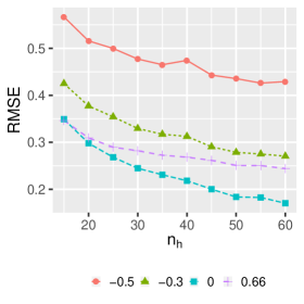
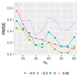
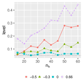
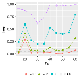
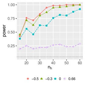
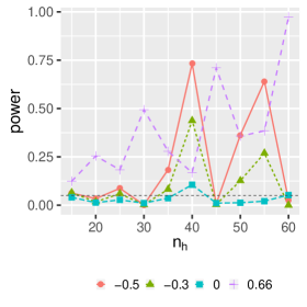
Figure 7: RMSEs (top), emprirical levels (middle) and empirical powers (bottom). Non-contaminated and contaminated settings (left and right, respectively). Random Clumped distribution

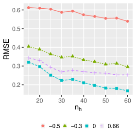
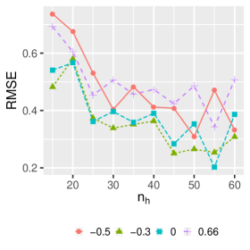
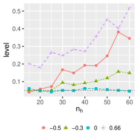
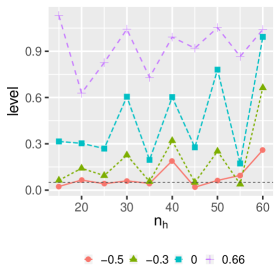
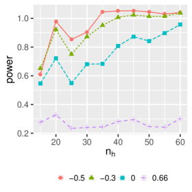
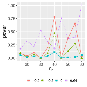
Figure 8: RMSEs (top), emprirical levels (middle) and empirical powers (bottom). Non-contaminated and contaminated settings (left and right, respectively). Dirichlet Multinomial distribution.

References

• Alonso-Revenga et al. (2017) J. Alonso-Revenga, N. Martín, and L. Pardo. New improved estimators for overdispersion in models with clustered multinomial data and unequal cluster sizes. Statistics and Computing, (27):193–217, 2017.
• Basak et al. (2020) S. Basak, A. Basu, and M. C. Jones. On the ‘optimal’ density power divergence tuning parameter. Journal of Applied Statistics, 0(0):1–21, 2020. doi: 10.1080/02664763.2020.1736524.
• Basu et al. (2017) A. Basu, A. Ghosh, A. Mandal, N. Martin, and L. Pardo. A Wald-type test statistic for testing linear hypothesis in logistic regression models based on minimum density power divergence estimator. Electronic Journal of Statistics, 11(2):2741–2772, 2017.
• Basu et al. (2018) A. Basu, A. Ghosh, A. Mandal, N. Martin, and L. Pardo. Robust Wald-type tests for non-homogeneous observations based on the minimum density power divergence estimator. Metrika, 81(5):493–522, 2018.
• Bertens et al. (2016) L. C. Bertens, K. G. Moons, F. H. Rutten, Y. van Mourik, A. W. Hoes, and J. B. Reitsma. A nomogram was developed to enhance the use of multinomial logistic regression modeling in diagnostic research. Journal of Clinical Epidemiology, 71:51–57, 2016.
• Binder (1983) D. A. Binder. On the variances of asymptotically normal estimators from complex surveys. International Statistical Review/Revue Internationale de Statistique, pages 279–292, 1983.
• Blizzard and Hosmer (2007) L. Blizzard and D. Hosmer. The log multinomial regression model for nominal outcomes with more than two attributes. Biometrical Journal, 49(6):889–902, 2007.
• Bull et al. (2007) S. B. Bull, J. P. Lewinger, and S. S. Lee. Confidence intervals for multinomial logistic regression in sparse data. Statistics in Medicine, 26(4):903–918, 2007.
• Castilla et al. (2018a) E. Castilla, A. Ghosh, N. Martín, and L. Pardo. New statistical robust procedures for polytomous logistic models. Biometrics, 74(4):1282–1291, 2018a.
• Castilla et al. (2018b) E. Castilla, N. Martín, and L. Pardo. Pseudo minimum phi-divergence estimator for the multinomial logistic regression model with complex sample design. Advances in Statistical Analysis, 102(3):381–411, 2018b.
• Castilla et al. (2018c) E. Castilla, N. Martín, and L. Pardo. A Logistic Regression Analysis Approach for Sample Survey Data Based on Phi-Divergence Measures, pages 465–474. Springer International Publishing, Cham, 2018c. ISBN 978-3-319-73848-2.
• Castilla et al. (2020) E. Castilla, A. Ghosh, N. Martín, and L. Pardo. Robust semiparametric inference for polytomous logistic regression with complex survey design. Advances in Data Analysis and Classification, 2020. DOI: 10.1007/s11634-020-00430-7.
• Cohen (1976) J. E. Cohen. The distribution of the chi-squared statistic under clustered sampling from contingency tables. Journal of the American Statistical Association, 71(355):665–670, 1976.
• Croux and Haesbroeck (2003) C. Croux and G. Haesbroeck. Implementing the Bianco and Yohai estimator for logistic regression. Computational Statistics and Data Analysis, 44(1-2):273–295, 2003.
• Daniels and Gatsonis (1997) M. J. Daniels and C. Gatsonis. Hierarchical polytomous regression models with applications to health services research. Statistics in Medicine, 16(20):2311–2325, 1997.
• Dreassi (2007) E. Dreassi. Polytomous disease mapping to detect uncommon risk factors for related diseases. Biometrical Journal, 49(4):520–529, 2007.
• Ghosh and Basu (2013) A. Ghosh and A. Basu. Robust estimation for independent non-homogeneous observations using density power divergence with applications to linear regression. Electronic Journal of Statistics, 7:2420–2456, 2013.
• Ghosh and Basu (2015) A. Ghosh and A. Basu. Robust estimation for non-homogeneous data and the selection of the optimal tuning parameter: the density power divergence approach. Journal of Applied Statistics, 42(9):2056–2072, 2015.
• Ghosh and Basu (2018) A. Ghosh and A. Basu. Robust bounded influence tests for independent non-homogeneous observations. Statistica Sinica, 28(3):1133–1155, 2018.
• Gupta et al. (2008) A. Gupta, T. Nguyen, and L. Pardo. Residuals for polytomous logistic regression models based on $\varphi$-divergences test statistics. Statistics, 42(6):495–514, 2008.
• Hampel et al. (1986) F. R. Hampel, E. M. Ronchetti, P. J. Rousseeuw, and W. A. Stahel. Robust statistics: the approach based on influence functions. John Wiley & Sons, 1986.
• Hosmer and Lemeshow (2000) D. W. Hosmer and S. Lemeshow. Applied logistic regression. John Wiley & Sons. New York, 2000.
• Johnson (1985) W. Johnson. Influence measures for logistic regression: Another point of view. Biometrika, 72(1):59–65, 1985.
• Ke et al. (2016) Y. Ke, B. Fu, and W. Zhang. Semi-varying coefficient multinomial logistic regression for disease progression risk prediction. Statistics in Medicine, 35(26):4764–4778, 2016.
• Lindsay et al. (1994) B. G. Lindsay et al. Efficiency versus robustness: the case for minimum hellinger distance and related methods. The Annals of Statistics, 22(2):1081–1114, 1994.
• Martín (2015) N. Martín. Using cook’s distance in polytomous logistic regression. British Journal of Mathematical and Statistical Psychology, 68(1):84–115, 2015.
• Martín and Pardo (2014) N. Martín and L. Pardo. New influence measures in polytomous logistic regression models based on phi-divergence measures. Communications in Statistics-Theory and Methods, 43(10-12):2311–2321, 2014.
• Morel (1989) J. G. Morel. Logistic regression under complex survey designs. Survey Methodology, 15(2):203–223, 1989.
• Morel and Nagaraj (1993) J. G. Morel and N. K. Nagaraj. A finite mixture distribution for modelling multinomial extra variation. Biometrika, 80(2):363–371, 1993.
• Morel and Neerchal (2012) J. G. Morel and N. K. Neerchal. Overdispersion models in SAS. SAS Publishing, 2012.
• Mosimann (1962) J. E. Mosimann. On the compound multinomial distributions, the multivariate b-distribution and correlation among proportions. Biometrika, 49:65–82, 1962.
• Office and Macro (2010) N. S. Office and I. Macro. Malawi demographic and health survey. Zomba, Malawi, and Calverton, Maryland, USA: NSO and ICF Macro, 2010.
• Pardo (2005) L. Pardo. Statistical inference based on divergence measures. CRC press, 2005.
• Roberts et al. (1987) G. Roberts, N. Rao, and S. Kumar. Logistic regression analysis of sample survey data. Biometrika, 74(1):1–12, 1987.
• Warwick and Jones (2005) J. Warwick and M. Jones. Choosing a robustness tuning parameter. Journal of Statistical Computation and Simulation, 75(7):581–588, 2005.