Removing biased data to improve fairness and accuracy

Abstract.

Machine learning systems are often trained using data collected from historical decisions. If past decisions were biased, then automated systems that learn from historical data will also be biased. We propose a black-box approach to identify and remove biased training data. Machine learning models trained on such debiased data (a subset of the original training data) have low individual discrimination, often 0%. These models also have greater accuracy and lower statistical disparity than models trained on the full historical data. We evaluated our methodology in experiments using 6 real-world datasets. Our approach outperformed seven previous approaches in terms of individual discrimination and accuracy.

1. Introduction

Automated decisions can be faster, cheaper, and less subjective than manual ones. In order to automate decisions, an organization can train a machine learning model on historical decisions or other manually-labeled data and use it to make decisions in the future. However, if the training data is biased, that bias will be reflected in the model’s decisions (Geiger et al., 2020; Coston et al., 2020). This problem has even been noted by the US White House (PODESTA, 2014).

Bias in models can have far-reaching societal consequences, like worsening wealth inequality (Hamilton, 2019), difference in employment rate across genders (Dastin, 2018; Martin, 2018), and difference in incarceration rates across races (Kaplan and Hardy, 2020). Discrimination has been reported in machine-produced decisions for real-life scenarios like parole (Julia Angwin and Kirchner, 2016), credit cards (Kopf, 2019), hiring (Dastin, 2018), and predictive policing (Goel et al., 2016). These problems are exacerbated by humans’ unwarranted confidence in machine-produced decisions: people generally deem such decisions fair (Dent, 2019). a Data bias happens mostly due to two phenomena: label bias and selection bias. Label bias occurs when the training labels (which are mostly generated manually) are afflicted by human bias. For example, loan applications and job applications from minority communities have been more frequently denied (Steil et al., 2017; Wikipedia contributors, 2020; Greenwood, 2020). Training on historical data would perpetuate that injustice. Selection bias occurs when selecting samples from a demographic group inadvertently introduces undesired correlations between the features pertaining to that demographic group and the training labels (Blum and Stangl, 2020; Yang et al., 2020; Wick et al., 2019), e.g. in the selected subsample for a group, most of their loan requests were denied. The propagation of bias has raised significant concerns related to use of machine learning models in critical decision making like the ones mentioned above.

Bias in machine learning systems is undesirable because it can produce unfair decisions (Dastin, 2018; Crosman, 2018), because biased decisions are less effective and less profitable (Kleinman, 2017; Alexandra, 2018), and because bias attracts lawsuits and widespread criticism (Kopf, 2019; Resnick, 2019). Biased decisions can be challenged on the basis of disparate treatment and disparate impact laws in the US (Barocas and Selbst, 2016; Jolly-Ryan, 2012; Selbst, 2017; Skeem and Lowenkamp, 2016; Winrow and Schieber, 2010). Similar laws exist in other countries (Australia, 2014). Laws define sensitive attributes (e.g., race, sex, religion) that are illegal to use as the basis of any decision.

We use both the common statistical disparity, and also individual discrimination as metrics to measure discrimination, in particular for machine learning classifiers. (Other definitions of fairness exist; section 5 justifies our choice.) A model is individually fair (Dwork et al., 2012) if it yields similar predictions for similar individuals. A similar pair consists of two individuals $\langle X,Y\rangle$ such that $X\neq Y$ and $X$ is similar to $Y$. Similarity among the individuals and among the predictions is measured by defining a distance function in the input space and the output space, respectively. A similar pair of individuals are two individuals with distance lower than a specified threshold. Ideally, for ensuring fairness, the input space similarity metric should not take sensitive features into account, so two individuals who differ only in the sensitive features should always be similar. A discriminatory pair is a similar pair such that the model makes dissimilar predictions for the two similar individuals. The individual discrimination of a model is the proportion of similar pairs of individuals that receive dissimilar predictions, i.e., the percentage of discriminatory pairs (Galhotra et al., 2017; Udeshi et al., 2018; Aggarwal et al., 2019). An estimate of individual discrimination uses a pool of similar pairs, which may be synthetically generated or sampled from the training data. To be fair, a model’s individual discrimination should be zero or close to it.

Previous approaches to reducing discrimination (see section 5) modify the training data’s features or labels (pre-processing), or add fairness regularizers while training (in-processing), or perform post-hoc corrections in the model’s predictions (post-processing).

Our approach is a pre-processing approach that identifies and removes biased datapoints from the training data, leaving all other datapoints unchanged. We conjectre that some training data is more biased than the rest and consequently has more influence on the predictions of a learned model. Influence functions (Koh and Liang, 2017) measure the influence of a training datapoint on a particular prediction. Our approach (1) generates discriminatory pairs (similar individuals who receive dissimilar predictions) and (2) uses influence functions to sort the training datapoints in order of most to least influential for the dissimilar predictions received by the discriminatory pairs. We hypothesize that the datapoints that are most responsible for the dissimilar predictions are the most biased datapoints. Removing the most influential datapoints yields a debiased dataset. A model trained on the debiased dataset is fairer with less individual discrimination — often 0% — than a model trained on the full dataset.

Our approach works for black-box classification models (for which only train and predict functions are available) (Card, 2017; Ncasas, 2017), and therefore proprietary models can be debiased as long as their training data is accessible. We performed 8 experiments using 6 real-world datasets (some datasets contain more than one sensitive attribute). Our approach outperforms seven previous approaches in terms of individual discrimination and accuracy and is near the average in terms of statistical disparity.

In summary, our contributions are:

• We propose a novel black-box approach for improving individual fairness: identify and remove biased decisions in historical data.

• In two sets of experiments using 6 real-world datasets, the classifiers trained on debiased datasets exhibit nearly 0% individual discrimination. Our approach outperforms seven previous approaches in terms of individual discrimination and accuracy, and it always improves (reduces) statistical disparity.

• To the best of our knowledge, we are the first to empirically demonstrate an increase in test accuracy (better generalization) in a supervised learning setup with real datasets while reducing discrimination, compared to the case when no fairness technique is used (Wick et al., 2019; Blum and Stangl, 2020).

• Our implementation and experimental scripts are open source.

2. Motivating Example

Table 1. A hypothetical dataset of past loan decisions. The second datapoint is a biased decision because a black person in high range income was denied a loan (0), whereas all white people with high range income were given a loan (1).

Id	Income	Wealth	Race	Decision
#1	1.0	0.1	White	1
#2	0.9	0.7	Black	0
#3	0.8	0.3	White	1
#4	0.1	0.7	Black	0
#5	0.1	0.5	White	0
#6	0.5	0.9	Black	0
#7	1.0	0.8	Black	1

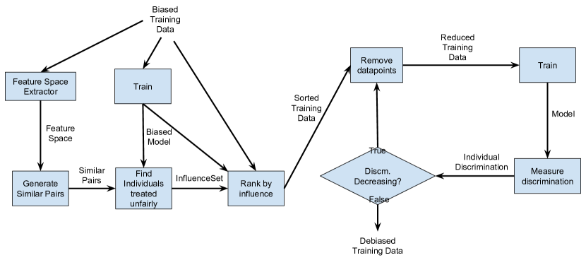
Figure 1. Flowchart with the steps in our approach. The left portion shows the steps in Algorithm 1 and the right portion shows the steps in Algorithm 2. The output of the algorithm is a debiased training data which can be used to train a debiased model.

Suppose that a bank wishes to automate the process of loan approval. The bank could train a machine learning model on historical loan decisions, then use the model to improve speed, reduce costs, and reduce subjectivity. The financial sector is a prominent user of machine learning (Techlabs, 2020; Didur, 2018).

Table 1 shows a hypothetical dataset consisting of historical loan decisions. The bank collects 3 features from each applicant: income, wealth, and race. As shown in the table, income and wealth are numeric features with values lying between 0 and 1, after normalization. Race is a binary feature with ‘white’ and ‘black’ as the two possible values. The outcome is also binary with ‘1’ indicating that a loan was offered and ‘0’ indicating a denial.

Loan approvals should ideally not depend on the applicant’s race, but past loan approvers might have been consciously or unconsciously biased. In fact, that was the case at this bank: #2 was a biased decision in which a black person with income in high range (0.9) was denied a loan, whereas all white people with high range income ($>$ 0.66) were given a loan. A classifier trained on a dataset that contains biased datapoints is likely to exhibit individual discrimination.

The bank would like to train a classifier using the unbiased parts of the historical data. Most of the decisions were probably sound (otherwise, the bank would have been out-competed by its rivals). It would be too expensive to filter biased decisions or create a new dataset manually, and those manual activities would also be prone to conscious and unconscious bias.

2.1. Measuring individual discrimination

Estimating a model’s individual discrimination requires the distance functions for the input and output space, and a pool of similar pairs. We consider two individuals similar if their income and wealth are the same, regardless of their race. We consider two decisions similar if they are the same decision. We randomly generate 700 similar pairs (see Section 3 for details). This is 100 times as large as the training dataset; the value “100” is arbitrary.

We trained a model on the dataset of table 1 and evaluated it on the 1400 individuals who form the 700 pairs of similar individuals. The model predicted different outcomes for 26% of the similar pairs (181 discriminatory pairs out of the 700 similar pairs).

2.2. Finding biased datapoints

Our goal is to find biased training datapoints, such that removing them reduces the model’s individual discrimination. This also improves the model’s accuracy and statistical parity, which is discussed in Section 4. Our approach contains three high-level steps:

1. Find unfair decisions made by a learned model. In particular, first generate a pool of pairs of similar individuals and find the discriminating pairs within them. Then, for each discriminating pair, heuristically determine which of the two individuals was not treated fairly.

2. Rank the training datapoints according to their contribution to the unfair decisions.

3. Remove some of the highest-ranked training datapoints and retrain a model with a lower individual discrimination.

Identify unfair decisions

There are 181 discriminatory pairs — pairs of similar individuals with dissimilar outcomes. One individual from each pair has been treated unfairly. The biased treatment might be in their favor (getting an undeserved loan) or against them (denied a loan they deserved). Our heuristic is that the individual whose classification confidence (i.e., the probability with which an individual is classified) is lower is the one who was treated unfairly. Note that these are the individuals in the generated pool of similar individuals, not in the training dataset.

Identify training datapoints responsible for unfair decisions

We use influence functions (Koh and Liang, 2017) to find the training datapoints that were most responsible for producing different predictions for the discriminatory pairs. An influence function sorts the training datapoints of a model in order of most to least responsible for a single prediction from the model. An influence function can also sort the datapoints for a set of predictions (the 181 unfair decisions, in our case), by measuring the average influence over all the relevant predictions.

We hypothesize that influence functions rank the training datapoints in order of most to least biased datapoints. Note that, the discriminatory pairs are only used to measure discrimination and to sort datapoints in the original training dataset; the discriminatory pairs themselves never occur in the training data.

For the dataset of table 1, the ranked datapoints are: #2, #7, #3, #1, #4, #6, #5. According to this ranking, #2 is the most biased decision, followed by #7 and so on.

Remove biased datapoints

When #2 is removed, and the model is retrained, it results in only 1 discriminatory pair out of the same 700 similar pairs of individuals, i.e., 0.14% remaining individual discrimination. When both #2 and #7 are removed, the discrimination is 16%. Therefore, removing only #2 is the local minimum for discrimination. Our algorithm returns the dataset with #2 removed. This reduced dataset is called the “debiased dataset”. Note that our approach removes biased datapoints from the training data. The similar pairs are synthetically generated and are only used to estimate individual discrimination and identify biased training points. The similar pairs can not be removed since they don’t occur in the training dataset.

The bank should train its model on the fair decisions in the debiased dataset, rather than on the whole dataset. We choose to remove the biased datapoint and not modify its label because the bias could arise either due to labeling bias or due to selection bias. Note that our approach can remove a datapoint belonging to any demographic group, not only the disadvantaged group as happened in this hypothetical dataset.

All the steps of our approach are shown in Figure 1.

Our approach requires access to sensitive attribute. Williams et al. (2018a); Veale and Binns (2017a) have argued about the necessity of having access to the sensitive features in order to identify and address bias in automated models. After identifying and removing the biased decisions, the bank can train their model by omitting the sensitive feature(s) (race in this case) to avoid disparate treatment (Jolly-Ryan, 2012).

Our approach empowers the bank to make less biased decisions in the future. (As with any automated decision-making process, the bank should include avenues for challenge and redress.) This avoids violating anti-discrimination laws and is the morally right thing to do.

3. Algorithm

Input : Training dataset D, Sensitive attribute S, Binary classification model M trained on D, Input space similarity threshold $\lambda$,

Output : D sorted in decreasing order of contribution to bias

1

2

3

4Function $\mathit{\textnormal{{SortDataset}}(\textnormal{{D}},\textnormal{{S}},\textnormal{{M}},\lambda})$

5       $\mathit{\textnormal{{PSI}}\leftarrow\textnormal{{GenerateSimilarPairs}}(\textnormal{{D}},\textnormal{{S}},\lambda)}$

       // Discriminating pairs: similar individuals who received dissimilar outcomes

6       $\mathit{\textnormal{{DP}}\leftarrow\{\langle i_{1},i_{2}\rangle\in\textnormal{{PSI}}:\textnormal{{M}}(i_{1})\neq\textnormal{{M}}(i_{2})\}}$

       // Individuals that M discriminates against

7       $\mathit{\textnormal{{InfluenceSet}}\leftarrow\{\}}$

8       for $\mathit{\langle i_{1},i_{2}\rangle\in\textnormal{{DP}}}$ do

             // Add to InfluenceSet the individual with lower classification confidence

9             if $\mathit{\textnormal{{Probability}}(i_{1})<\textnormal{{Probability}}(i_{2})}$  then

10                  $\mathit{\textnormal{{InfluenceSet}}\leftarrow\textnormal{{InfluenceSet}}\cup\langle i_{1},\textnormal{{M}}(i_{1})\rangle}$

11            else

12                  $\mathit{\textnormal{{InfluenceSet}}\leftarrow\textnormal{{InfluenceSet}}\cup\langle i_{2},\textnormal{{M}}(i_{2})\rangle}$

13            

14       return RankByInfluence (InfluenceSet, D)

// Randomly generates pairs of similar individuals

15

16Function $\mathit{\textnormal{{GenerateSimilarPairs}}(\textnormal{{D}},\textnormal{{S}},\lambda)}$

17       $\mathit{\textnormal{{SimilarPairs}}\leftarrow\{\}}$

18       for $\mathit{i\leftarrow 1\ \textnormal{{to}}\ 100*|D|}$ do

             $\mathit{A1}\leftarrow\textnormal{{Sample}}(\textnormal{{D}})$ // Sample from feature space

             $\mathit{A2}\leftarrow\textnormal{{SimilarIndividual}}(\textnormal{{D}},A1,\textnormal{{S}},\lambda)$ // Generate A2 s.t. distance(A1, A2) $<\lambda$

19             $\mathit{\textnormal{{SimilarPairs}}\leftarrow\textnormal{{SimilarPairs}}\cup\langle A1,A2\rangle}$

20            

21      return SimilarPairs

// Ranks datapoints in D responsible for discrimination, sorted in decreasing order of influence

22 Function $\mathit{\textnormal{{RankByInfluence}}(\textnormal{{InfluenceSet}},\textnormal{{D}})}$

       // See (Koh and Liang, 2017) for implementation

23      

Algorithm 1 Sort the training data in decreasing order of bias

Input : Training dataset D, Sensitive attribute S, Input space threshold $\lambda$, Train function

Output : Debiased version of D, which is a subset of D

1

2

3Function $\mathit{\textnormal{{DebiasData}}(\textnormal{{D}},\textnormal{{S}},\lambda,\textnormal{{Train}})}$

       // Model trained on full dataset

4       $\mathit{\textnormal{{M}}_{\mathrm{full}}\leftarrow\textnormal{{Train}}(\textnormal{{D}})}$

       // Sorted biased datapoints (see algorithm 1)

5       $\mathit{\textnormal{{SD}}\leftarrow\textnormal{{SortDataset}}(\textnormal{{D}},\textnormal{{S}},\textnormal{{M}}_{\mathrm{full}},\lambda)}$

6       $\textnormal{{LeastDiscrim}}\leftarrow\infty$

7       for $\mathit{i\leftarrow}$ 0 to 100 do

             // Model trained on remaining data

             $\mathit{\textnormal{{M}}\leftarrow\textnormal{{Train}}(\textnormal{{DropFirst}}(\textnormal{{SD}},i))}$ // DropFirst removes the first i% from input dataset SD

8             $\mathit{\textnormal{{Discrim}}\leftarrow\textnormal{{EstimateDiscrim}}(\textnormal{{M}},\textnormal{{D}},\textnormal{{S}},\lambda)}$

9             if $\mathit{\textnormal{{Discrim}}\geq\textnormal{{LeastDiscrim}}}$ then

10                  return $\textnormal{{DropFirst}}(\textnormal{{SD}},i-1)$

11            

12            $\mathit{\textnormal{{LeastDiscrim}}\leftarrow\textnormal{{Discrim}}}$

// Estimates the individual discrimination of model M

13 Function $\mathit{\textnormal{{EstimateDiscrim}}(\textnormal{{M}},\textnormal{{D}},\textnormal{{S}},\lambda)}$

14       $\textnormal{{PSI}}\leftarrow\textnormal{{GenerateSimilarPairs}}(\textnormal{{D}},\textnormal{{S}},\lambda)$

       // Discriminating pairs: similar individuals who received dissimilar outcomes

15       $\textnormal{{DP}}\leftarrow\{\langle i_{1},i_{2}\rangle\in\textnormal{{PSI}}:\textnormal{{M}}(i_{1})\neq\textnormal{{M}}(i_{2})\}$

16       return $|\textnormal{{DP}}|\,/\,|\textnormal{{PSI}}|$

Algorithm 2 Produce a debiased dataset

Algorithm 1 sorts a dataset in the order of most biased to least biased datapoint. It has four main parts.

First, algorithm 1 generates a pool PSI of pairs of similar individuals using GenerateSimilarPairs (algorithm 1). We arbitrarily choose the size of the pool to be 100 times the size of the dataset. A larger pool leads to a better estimate of individual discrimination. The individuals and their similar counterparts are automatically generated, sampling uniformly at random from the feature space that is defined by the original training dataset. For a randomly sampled individual A1, SimilarIndividual (algorithm 1) generates a similar individual A2 whose distance from A1 is less than the specified threshold $\lambda$, which is a user-provided parameter that determines whether two individuals are similar. For the input space similarity condition in Section 2, $\lambda$ is 0. For example, random sampling for income, wealth, and race in the hypothetical dataset could generate an individual A1 with the feature vector $\langle 0.9,0.5,White\rangle$. According to the input space similarity condition, a similar individual for A1 must have the same income and wealth (these are the non-sensitive features). While generating similar individuals, we enforce changing the value of the sensitive attribute (race in this case) to generate similar individuals in different demographic groups. Therefore, A2 has the feature vector $\langle 0.9,0.5,Black\rangle$. These pairs of similar individuals allow us to estimate the individual discrimination of a model because we can compare their predictions, which should be similar as well. Note that generating pairs of similar individuals based on a given $\lambda$, as opposed to finding pairs of similar individuals in the training dataset, allows us to reliably generate a large pool of pairs.

Second, algorithm 1 determines the discriminatory pairs: the pairs of similar individuals who received dissimilar model predictions (a subset of the pool PSI). In the case of binary classification, different labels are considered dissimilar.

Third, algorithms 1 to 1 determine, for each discriminatory pair, which individual was misclassified due to model bias. Internally, a classifier computes, for each outcome class, the probability of an individual belonging to that class, and the predicted outcome for that individual is the class with the highest probability. Classification confidence refers to this highest probability. Our heuristic (algorithm 1) is that the individual with the lower classification confidence is the one who was treated unfairly.

Fourth, RankByInfluence (algorithm 1) identifies the datapoints in the original (biased) training dataset D responsible for discrimination against these individuals. Given a trained model and a set of datapoints along with their predictions from the model, RankByInfluence ranks the training data of the model from most influential to least influential training datapoint responsible for those predictions. If the most influential datapoints are removed from the training data, and the model is retrained with the same model architecture, the probability of change in the prediction of the discriminatory pairs is highest. We hypothesize that RankByInfluence returns the training datapoints sorted in order of most to least bias, and our experiments support this. We show all the four steps in the left portion of Figure 1.

None of the above steps is dependent on the number of output categories, so the algorithm is applicable to multi-class classifiers. The notion of similar predictions would need to be adjusted accordingly.

Algorithm 2 first calls SortDataset to rank the datapoints in decreasing order of bias (algorithm 2). It then iteratively removes a chunk of the most biased datapoints from the sorted original training dataset (algorithm 2), retrains the same model architecture on the remaining datapoints, and estimates the individual discrimination of the retrained model (algorithm 2). When the remaining discrimination in a retrained model reaches a local minimum, it returns a debiased dataset by dropping the most biased datapoints from the original training data (algorithm 2). The size of each chunk can be adjusted as desired (it is 1/100 of the original training data in algorithm 2).

4. Evaluation

Table 2. Datasets used in the evaluation

Id	Dataset	Size	# Numerical Attrs.	# Categorical Attrs.	Sensitive Attr. (S)	Training label (binary)
D1	Adult income (Dua and Graff, 2017a)	45222	1	11	Sex	Income $\geq$ $50K
D2	Adult income (Dua and Graff, 2017a)	43131	1	11	Race	Income $\geq$ $50K
D3	German credit (Dua and Graff, 2017c)	1000	3	17	Sex	Credit worthiness
D4	Student (Dua and Graff, 2017d)	649	4	28	Sex	Exam score $\geq$ 11
D5	Recidivism (Jeff Larson and Angwin, 2016)	6150	7	3	Race	Ground-truth recidivism
D6	Recidivism (Jeff Larson and Angwin, 2016)	6150	7	3	Race	Prediction of recidivism
D7	Credit default (Dua and Graff, 2017b)	30000	14	9	Sex	Credit worthiness
D8	Salary  (Rodriguez, 2020)	52	2	3	Sex	Salary $\geq$ $23719

We conducted experiments to answer the following research questions:

RQ1:

Does our technique reduce individual discrimination?

RQ2:

Do previous techniques reduce individual discrimination?

RQ3:

How does our technique impact test accuracy?

RQ4:

How do previous techniques impact test accuracy?

RQ5:

How do the techniques compare in terms of statistical disparity?

RQ6:

How sensitive are the techniques to hyperparameter choices?

We compared our pre-processing technique against 7 other techniques: a baseline model trained on the full training dataset (Full), five pre-processing techniques — simple removal of the sensitive attribute (SR), Disparate Impact Removal (DIR) (Feldman et al., 2015) (used at the highest fairness enforcing level, repair=1), Preferential Sampling (PS) (Kamiran and Calders, 2012), Massaging (MA) (Kamiran and Calders, 2012), and Learning Fair Representations (LFR) (Zemel et al., 2013) — and one in-processing technique — Adversarial Debiasing (AD) (Zhang et al., 2018). The implementations for some of these techniques were taken from IBM AIF360 (Bellamy et al., 2018).

We evaluated the techniques using six real-world datasets that are commonly used in the fairness literature (see table 2).

For all experiments, the machine learning model architecture we used was a neural network with 2 hidden layers. We trained models with 240 different hyperparameter settings:

• In the first hidden layer, the number of neurons is 16, 24, or 32.

• In the second hidden layer, the number of neurons is 8 or 12.

• Each model had two choices for batch sizes: the closest powers of 2 to the numbers obtained by dividing the dataset size by 10 and 20, respectively. For example, if the dataset size is 1000, the batchsizes are 64 and 128.

• Each experiment had 20 choices for random permutations for the full dataset. The choice of random permutation affects the datapoints that form the training and test datasets.

4.1. Experimental methodology

To create the models for our approach (to answer RQ1 and RQ3), we executed the following methodology:

1. For each of the 240 choices of hyperparameters:

   1. Split the dataset into the first 80% training and last 20% testing (without randomness, but depending on the data permutation, which is one of the hyperparameters). The dataset is normalized before usage.

   2. Debias the training dataset using Algorithm 2; that is, remove some points from it.

   3. Compute a “debiased model”, which is trained on the debiased training dataset.

2. Let the “unfair datapoints” for a dataset be the union of the datapoints removed by all the 240 models: that is, any datapoint removed by any debiasing step.

To create the models for other approaches (to answer RQ2 and RQ4), we ran each approach 240 times, once for each choice of hyperparameters. The in-processing technique AD (Zhang et al., 2018) does not take hyperparameters other than data permutations, therefore we only repeated the process 20 times, once for each data permutation.

To measure the performance of the models, we executed the following methodology for each trained model:

1. Measure the model’s individual discrimination using the function DiscmTest of Algorithm 2 (RQ1 and RQ2).

2. Measure the model’s test accuracy on a debiased test set (RQ3 and RQ4). The debiased test set is computed by removing the unfair points from the test set, which is the last 20% of the dataset.

Note that when evaluating our technique, the points removed from the test set of a model is not affected by that model itself, but only by other models that have those test points in their training set. Thus, there is no leak between the training and test dataset. The fourth hyperparameter, random perturbation, affects the datapoints that form the training and test datapoints for a model.

We conducted two sets of experiments (sections 4.2 and 4.3) with different similarity conditions in the input space.

4.1.1. Debiasing the test set

Our evaluation methodology uses a debiased test set from which unfair points have been removed. The reason is that a user’s goal is not to obtain a model that performs well on the entire dataset that includes biased decisions, but a model that performs well on fair decisions. Our experimental results indicate that our debiasing technique identifies fair decisions, so we use it for this purpose.

This experimental methodology addresses an observation made by Wick et al. (2019) that in most previous discrimination mitigation approaches, there is a discrepancy between the algorithm and its evaluation. Previous authors have agreed on the existence of bias in the data and have devised algorithms to mitigate bias in the resulting data or classifier, but they evaluated the accuracy of their approach on the original test set, which is potentially biased. Due to this discrepancy, most previous work suggests that a technique must trade off fairness and accuracy (Berk et al., 2017; Chouldechova, 2017; Corbett-Davies et al., 2017; Feldman et al., 2015; Fish et al., 2016; Kamiran and Calders, 2012; Kleinberg et al., 2016; Menon and Williamson, 2018; Zafar et al., 2017a; Calmon et al., 2017; Calders and Verwer, 2010; Kamishima et al., 2012), which Wick et al. (2019) refute.

Using our experimental methodology, the classifier debiased using our approach usually has higher accuracy on the debiased test set than the classifier trained on the full dataset (see sections 4.4 and 4.5). We think of this phenomenon as a classifier with improved generalization, an intuition also shared by Berk et al. (2017), who remark that fairness constraints might act as regularizers and improve generalization.

Another advantage is that using the same test set for a particular set of hyperparameters provides an apples-to-apples comparison of our technique with all the seven baselines. For the Full baseline, the full training set is used, while the test set is still debiased.

4.2. Experiments with input space threshold $\lambda$=0

In the first set of experiments we used the following distance functions with the definitions of individual discrimination.

Input space similarity condition: We consider two individuals to be similar if they are the same in all non-sensitive features.

Output space similarity condition: We consider two outcomes to be similar if they are the same outcome. Note that for all our experiments, the outcomes are binary.

Generating similar individuals: For the given similarity condition in the input space, GenerateSimilarPairs randomly generates the first individual, and then flips its sensitive feature to generate an individual similar to it (similar procedure as used for the hypothetical dataset in Section 2). For example, the Salary dataset has features sex, rank, age, degree, and experience, out of which age and experience are numerical while the others are categorical features. If the first randomly generated individual had feature values $\langle$Male, Full, 35, Doctorate, 5$\rangle$, then the similar individual would have feature values $\langle$Female, Full, 35, Doctorate, 5$\rangle$. In this set of experiments, the number of pairs of similar individuals generated for each dataset was set to 100 times the size of the respective total dataset (e.g., 3,000,000 for the Credit default dataset).

When generating individuals, there is no guarantee that the generated individuals are representative of the actual population. For example, consider a dataset whose features include gender and college alma mater. It might generate a datapoint for a male who graduated from a women’s college. Such individuals are uncommon (Timothy Boatwright of Wellesley College is one example). Therefore, a dataset with many such individuals might or might not be useful in determining whether there is discrimination against graduates of the women’s college. As another example, consider determining whether a basketball coach has discriminated ethnically in selecting team members; generated individuals might not be representative since Bolivian men have an average height of 160cm (5’1"), and Bosnian men have an average height of 184cm (6’). Data selection (as opposed to generation) approaches can guarantee that the individuals are characteristic, but they require accurate characterizations of, or large samples from, the population (which we don’t have access to). Even so, it may not be possible or easy to find many similar pairs of individuals to compare. We acknowledge these limitations. Future work should explore how to obtain similar pairs that are characteristic of real-world populations.

4.3. Experiments with input space threshold $\lambda$$>$0

The second set of experiments used these distance functions.

Input space similarity condition: We consider two individuals to be similar if, among the non-sensitive features, they have the same value for all categorical features and are within a 10% range for all numerical features (after normalization).

Output space similarity condition: We consider two outcomes similar if they are the same outcome.

Generating similar individuals: GenerateSimilarPairs randomly generates the first individual A1. It then generates 2 similar individuals for A1 following the input space similarity condition. (Therefore, in this set of experiments, the size of the pool of similar pairs was equal to 200 times the size of the dataset.) A similar individual is generated by maintaining the same values for all categorical features, and random sampling within the $-10$% to $+10$% range for all numerical features.

Table 3. Information about the model with the least remaining discrimination, among 240 hyperparameter settings when $\lambda=0$. All numbers are percentages.

	Individual discrimination								Test accuracy								Statistical parity difference
Id	Full	SR	DIR	PS	MA	LFR	AD	Our	Full	SR	DIR	PS	MA	LFR	AD	Our	Full	SR	DIR	PS	MA	LFR	AD	Our
D1	19.0	0.0	19.0	0.0064	5.7	0.096	12.0	0.0	80	82	80	81	80	81	85	92	29	13	28	8.7	3.3	3.6	2.3	7.8
D2	11.0	0.0	11.0	0.38	6.0	0.0063	4.3	0.0	83	85	84	84	83	84	87	92	21	13	20	12	7	0.33	7.8	10
D3	6.2	0.0	3.8	0.014	0.083	0.0	8.1	0.0	75	82	74	73	75	62	76	81	1.6	3.1	2.1	14	6.2	0.085	1.5	9.8
D4	0.0015	0.0	0.02	0.0	3.5	0.037	2.3	0.0	96	98	95	92	92	69	92	96	15	5.7	20	12	13	3.8	11	25
D5	0.013	0.0	0.0046	0.11	0.87	0.0	0.34	0.0	73	77	62	48	76	73	76	74	21	26	33	2.3	3.7	0.0	0.96	25
D6	0.045	0.0	0.0046	0.02	0.16	9.8e-4	0.01	0.0	67	81	49	65	78	78	79	84	39	25	49	14	1.1	22	26	23
D7	1.2	0.0	0.04	0.65	1.3	0.0	0.046	0.0	76	78	71	77	75	83	85	80	12	6.1	11	1.6	4.6	0.0	3.4	0.12
D8	0.019	0.0	0.0	0.019	19.0	0.0	33.0	0.0	100	100	100	100	100	50	75	100	33	11	12	22	50	0.0	0.0	0.0
Avg.	4.7	0.0	4.2	0.15	4.6	0.018	7.5	0.0	81	85	76	77	82	72	81	87	21	13	22	11	11	3.7	6.6	13

Table 4. Information about the model with highest test accuracy, among 240 hyperparameter settings when $\lambda=0$. All numbers are percentages.

	Individual discrimination								Test accuracy								Statistical parity difference
Id	Full	SR	DIR	PS	MA	LFR	AD	Our	Full	SR	DIR	PS	MA	LFR	AD	Our	Full	SR	DIR	PS	MA	LFR	AD	Our
D1	21.0	0.0	21.0	0.73	6.3	4.5	17.0	6.6e-5	82	82	82	82	82	83	85	93	29	13	29	11	1.5	3.3	0.18	9.9
D2	12.0	0.0	12.0	1.8	8.0	0.42	5.2	9.3e-5	85	85	85	85	85	85	88	92	22	13	21	11	5.4	0.18	0.37	13
D3	11.0	0.0	8.7	1.1	1.7	0.56	11.0	0.007	82	82	81	83	85	78	82	82	11	3.1	6.1	3.2	1.2	2.6	5	7.9
D4	0.94	0.0	0.44	0.85	6.2	1.7	3.3	0.0031	98	98	98	99	98	89	96	98	18	5.7	20	2.4	8	16	12	17
D5	0.094	0.0	0.044	0.64	2.4	0.044	0.5	0.0016	77	77	72	61	85	87	80	100	32	26	38	3.9	1.6	21	22	26
D6	0.05	0.0	0.011	0.028	0.5	3.0	0.037	0.0013	74	81	50	76	87	83	81	100	38	25	48	15	0.078	22	26	26
D7	1.4	0.0	0.12	0.77	1.5	2.8	0.24	0.0	78	78	75	78	78	85	85	80	13	6.1	9	2.1	1.2	2	2.3	3.4
D8	0.019	0.0	0.0	0.019	19.0	6.8	33.0	0.0	100	100	100	100	100	100	75	100	11	11	10	10	0.0	12	0.0	10
Avg.	5.8	0.0	5.3	0.74	5.7	2.5	8.8	0.0016	84	85	80	83	87	86	84	93	22	13	23	7.3	2.4	9.9	8.5	14

Table 5. Information about the model with least statistical parity difference, among 240 hyperparameter settings when $\lambda=0$. All numbers are percentages.

	Individual discrimination								Test accuracy								Statistical parity difference
Id	Full	SR	DIR	PS	MA	LFR	AD	Our	Full	SR	DIR	PS	MA	LFR	AD	Our	Full	SR	DIR	PS	MA	LFR	AD	Our
D1	20.0	0.0	20.0	0.1	6.7	5.2	17.0	2.2e-5	81	81	81	81	80	82	85	92	28	12	27	8.7	0.013	0.013	0.18	7.1
D2	13.0	0.0	13.0	1.8	7.5	0.025	5.3	4.2e-4	84	84	85	85	84	84	88	91	18	7.9	18	5	0.28	0.0024	0.37	7.6
D3	7.6	0.0	9.1	2.0	1.2	0.39	9.1	0.24	78	82	76	76	71	72	80	74	0.32	0.22	0.026	0.25	0.0	0.0	0.19	0.016
D4	3.9	0.0	3.6	1.2	7.1	5.5	4.6	0.0046	93	96	92	93	90	77	89	94	0.27	0.075	0.39	0.075	0.077	0.15	1.1	0.075
D5	0.085	0.0	0.014	0.24	1.5	0.0	0.34	0.0059	67	75	64	44	81	73	76	100	20	17	26	0.019	0.011	0.0	0.96	12
D6	0.049	0.0	0.0083	0.032	0.25	0.041	0.013	0.0021	72	78	48	68	82	71	77	100	33	19	42	9.6	0.0013	18	5.5	16
D7	1.2	0.0	0.071	0.98	1.4	0.0	0.49	0.0	76	77	73	77	78	83	84	77	8.9	3	8.3	0.022	0.14	0.0	0.62	0.12
D8	1.0	0.0	2.2	0.038	25.0	0.0	33.0	0.0	100	100	100	100	100	100	71	100	0.0	0.0	0.0	0.0	0.0	0.0	0.0	0.0
Avg.	5.9	0.0	6.0	0.8	6.3	1.4	8.7	0.032	81	84	77	78	83	80	81	91	14	7.4	15	3	0.065	2.3	1.1	5.4

4.4. Results for input space threshold $\lambda$ = 0

The left portion of section 4.3 reports, for each technique, the best (lowest) individual discrimination among its 240 models. (Figure 2 plots, for each technique, the individual discrimination of all 240 models.) When multiple models have the lowest discrimination, we choose the model with the highest accuracy. Answer to RQ1: For all datasets, our technique achieves 0% remaining discrimination. Answer to RQ2: SR also achieves 0% individual discrimination. This follows from our choice of input space similarity condition. When the sensitive feature is removed, the remaining features are the same for all pairs of similar individuals. And therefore, SR gives the same prediction for two individuals with the same features. LFR and PS leave little remaining discrimination. The other techniques (DIR, MA, and AD) are not effective in eliminating individual discrimination.

The center portion of section 4.3 reports, for each technique, the accuracy of the lowest-discrimination model. Answer to RQ3: Our technique produces models with better accuracy than models trained on the entire training dataset. This agrees with the observation made by Wick et al. (2019): “it requires no stretch of credulity to imagine that various personal attributes (e.g., race, gender, religion; sometimes termed ‘protected attributes’) have no bearing on a person’s intelligence, capability, potential, qualifications, etc., and consequently no bearing on the ground truth classification labels — such as job qualification status — that might be functions of these qualities. It then follows that enforcing fairness across these attributes should on average increase accuracy.” Answer to RQ4: DIR, PS, and LFR degrade the accuracy; AD and MA affect it little; and SR improves it, though not as much as our technique does. Our approach is always either best or within 3 percentage points of best, and is best on average.

A user may train multiple models (e.g., using different hyperparameter choices) and choose the best one for their application. Section 4.3 assumes that the user chooses the least-discriminating model. Section 4.3, by contrast, assumes that the user chooses the most accurate model. And section 4.3 assumes that the user chooses the model with the least statistical disparity. These are the extremal points on the Pareto frontier; a user might also choose a point between them (Hu and Chen, 2020).

The left and center portions of section 4.3 report, for each technique, the individual discrimination and accuracy of the most accurate model among the 240 models. We can answer RQ1–RQ4 about these models. Answer to RQ1 and RQ2: Our approach achieves, on average, nearly 0% (0.0016%) remaining discrimination; under the definition of our input space similarity condition, SR achieves 0% discrimination; other techniques are much higher. Answer to RQ3 and RQ4: Our approach achieves by far the highest average accuracy: 93% compared to the Full model’s 84% accuracy and MA’s 87% accuracy.

Table 6. Information about the model with the least remaining discrimination, among 240 hyperparameter settings when $\lambda>0$. All numbers are percentages.

	Individual discrimination								Test accuracy								Statistical parity difference
Id	Full	SR	DIR	PS	MA	LFR	AD	Our	Full	SR	DIR	PS	MA	LFR	AD	Our	Full	SR	DIR	PS	MA	LFR	AD	Our
D1	19.0	0.0026	19.0	0.042	5.6	0.41	12.0	0.62	81	83	81	85	81	84	85	86	29	15	28	8.9	3.3	3.6	2.3	9.8
D2	11.0	0.00044	11.0	0.45	6.0	0.37	4.3	0.67	79	80	80	80	79	80	85	81	21	8.1	20	12	7	0.59	7.8	12
D3	6.4	1.9	4.2	2.2	2.0	0.066	8.7	1.6	75	81	74	73	76	62	76	82	1.6	1.1	2.1	2.1	3.3	2.7	1.5	7.6
D4	4.7	4.6	4.8	4.7	4.2	0.87	4.5	2.3	99	98	100	98	96	90	98	97	13	12	6.6	13	12	5.4	11	4.4
D5	0.19	0.2	0.0052	0.14	0.97	0.0	0.36	8.1e$-$5	63	62	60	44	63	70	64	100	26	24	33	2.4	3.7	0.0	8.4	0.72
D6	0.048	0.046	0.0033	0.033	0.21	0.18	0.0088	0.0002	60	67	49	59	72	72	67	99	38	23	47	14	1.1	21	26	26
D7	1.8	1.6	0.19	1.5	1.9	0.0	0.079	0.0	76	76	71	76	75	86	85	83	12	4.7	11	1.4	4.6	0.0	3.4	6.5
D8	1.7	1.3	0.033	1.5	19.0	0.0	33.0	0.0	100	100	100	100	100	57	75	100	0.0	0.0	30	0.0	50	0.0	0.0	30
Avg.	5.6	1.2	4.9	1.3	5.0	0.24	7.9	0.65	79	80	76	76	80	75	79	91	18	11	22	6.7	11	4.2	7.5	12

Table 7. Information about the model with highest test accuracy, among 240 hyperparameter settings when $\lambda>0$. All numbers are percentages.

	Individual discrimination								Test accuracy								Statistical parity difference
Id	Full	SR	DIR	PS	MA	LFR	AD	Our	Full	SR	DIR	PS	MA	LFR	AD	Our	Full	SR	DIR	PS	MA	LFR	AD	Our
D1	20.0	0.11	21.0	0.5	6.2	4.5	17.0	0.62	82	84	82	85	82	85	85	86	29	13	29	11	1.5	3.3	0.18	12
D2	12.0	0.22	12.0	1.8	7.7	0.81	5.3	0.89	80	81	81	81	81	80	87	82	22	13	21	11	5.4	0.18	0.37	14
D3	11.0	2.1	8.7	2.6	2.7	1.1	11.0	1.6	82	82	81	83	85	78	83	82	11	3.1	6.1	3.2	1.2	2.6	5	5.8
D4	5.1	4.8	4.8	4.9	5.0	2.8	5.1	2.7	100	100	100	100	100	96	100	100	18	5.7	20	2.4	8	16	12	16
D5	0.58	0.57	0.065	0.71	2.6	4.8	0.61	8.1e$-$5	75	74	74	55	75	87	67	100	32	26	38	3.9	1.6	21	22	28
D6	0.054	0.06	0.01	0.11	0.59	5.4	0.034	0.00021	66	74	50	70	82	81	75	100	38	25	48	15	0.078	22	26	19
D7	2.0	1.7	0.62	1.7	2.1	3.7	0.26	0.0	78	78	75	79	78	87	85	83	13	6.1	9	2.1	1.2	2	2.3	12
D8	1.7	1.3	0.033	1.5	19.0	7.3	33.0	0.0	100	100	100	100	100	100	75	100	11	11	10	10	0.0	12	0.0	10
Avg.	6.6	1.4	5.9	1.7	5.7	3.8	9.0	0.73	82	84	80	81	85	86	82	91	22	13	23	7.3	2.4	9.9	8.5	15

Table 8. Information about the model with least statistical parity difference, among 240 hyperparameter settings when $\lambda>0$. All numbers are percentages.

	Individual discrimination								Test accuracy								Statistical parity difference
Id	Full	SR	DIR	PS	MA	LFR	AD	Our	Full	SR	DIR	PS	MA	LFR	AD	Our	Full	SR	DIR	PS	MA	LFR	AD	Our
D1	20.0	0.11	20.0	0.1	6.7	5.2	17.0	0.75	81	84	82	85	81	82	85	85	28	12	27	8.7	0.013	0.013	0.18	8.8
D2	13.0	0.22	13.0	1.8	7.5	1.1	5.3	1.2	79	79	80	80	79	79	87	81	18	7.9	18	5	0.28	0.0024	0.37	9
D3	7.8	2.6	9.1	3.0	3.3	1.5	9.5	2.8	79	82	75	77	71	73	80	78	0.32	0.22	0.026	0.25	0.0	0.0	0.19	0.095
D4	6.0	5.3	5.9	5.4	7.2	5.9	6.2	4.2	99	99	99	99	97	79	98	99	0.27	0.075	0.39	0.075	0.077	0.15	1.1	0.075
D5	0.32	0.41	0.021	0.28	1.7	0.0	0.38	9.8e$-$5	63	64	62	44	72	70	65	100	20	17	26	0.019	0.011	0.0	0.96	0.044
D6	0.052	0.061	0.0088	0.058	0.31	0.46	0.014	0.00023	66	70	48	64	78	70	74	99	33	19	42	9.6	0.0013	18	5.5	17
D7	2.1	1.9	0.46	1.9	2.2	0.0	0.65	0.0	76	75	73	78	78	86	84	81	8.9	3	8.3	0.022	0.14	0.0	0.62	6.5
D8	1.7	1.3	2.2	1.5	25.0	0.0	33.0	0.86	100	100	100	100	100	100	75	100	0.0	0.0	0.0	0.0	0.0	0.0	0.0	0.0
Avg.	6.4	1.5	6.3	1.8	6.7	1.8	9.0	1.2	80	81	77	78	82	79	81	90	14	7.4	15	3	0.065	2.3	1.1	5.2

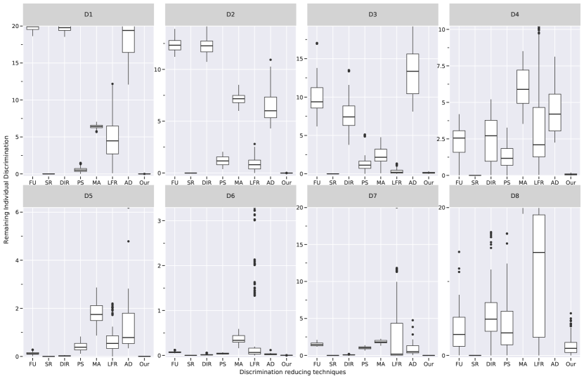
Figure 2. The individual discrimination for all 240 hyperparameter choices (lower is better). Our approach (rightmost in each boxplot) always achieves 0% discrimination for some (often many) hyperparameter choices, and it has a little variance across choices.

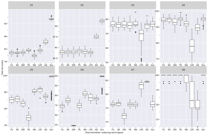
Figure 3. The test accuracy for all 240 hyperparameter choices (higher is better). Our approach is best or comparable to the best in terms of both accuracy and its variance, for all experiments except D7.

We also measured the statistical disparity: the absolute difference between the success rate for individuals with one value for the sensitive attribute and the success rate for individuals with the other value for the sensitive attribute. The right portions of sections 4.3, 4.3 and 4.3 report the results. Answer to RQ5: Our technique achieves a lower statistical disparity than the baseline model trained on the full dataset. Compared to the other techniques (which are designed to optimize for statistical parity difference), our technique is in the middle of the pack. For each technique that has a lower statistical disparity than ours, our technique achieves considerably lower individual discrimination and higher accuracy.

If a bias mitigation technique is highly sensitive to hyperparameter choices, then users might need to run it many times to achieve desirable performance, and they may have less confidence in its generalizability.

Figure 2 shows the remaining individual discrimination for all 240 models we trained for each experiment and each technique, and fig. 3 shows the test accuracy for all the 240 models for each experiment and each technique.

Answer to RQ6: Our technique not only usually results in lower remaining discrimination and higher accuracy than previous techniques, it is also much less sensitive to hyperparameter choices (narrower range).

4.5. Results for input space threshold $\lambda$ $>$ 0

Sections 4.4, 4.4 and 4.4 report the same statistics for the experiment with $\lambda>0$. We answer RQ1-RQ4 using Section 4.4 and Section 4.4.

Answer to RQ1: For both the models with the least discrimination and highest accuracy, our approach achieves very low individual discrimination (0.65% and 0.73% respectively).

Answer to RQ2: For the most accurate model, our approach gets the lowest discrimination among all approaches (0.73%). For the models with the least discrimination, our approach is second and very close to the best performing approach (LFR). Notably, SR has much higher discrimination for this choice of similarity metric. In the previous set of experiments, SR was able to get 0% individual discrimination just by choice of input space similarity.

Answer to RQ3: Our approach gets the best accuracy by far compared to all the baselines for both the models with the least discrimination and highest accuracy.

Answer to RQ4: Similar to the conclusions from the experiments with $\lambda=0$, for the least discriminative model: DIR, PS, and LFR degrade the accuracy; AD, MA, and SR affect it little. For the most accurate model: SR, MA, and LFR improve the accuracy but not as much as our approach.

Answer to RQ5: For statistical disparity (shown in the right portions of sections 4.4, 4.4 and 4.4) the conclusions are the same as when $\lambda=0$.

Answer to RQ6: Due to lack of space, we have added the plots showing the remaining discrimination and test accuracy for the experiments with $\lambda>0$ in the appendix (Appendix A). The conclusions are the same as when $\lambda=0$.

5. Related Work

5.1. Fairness Metrics

More than 20 metrics for fairness have been proposed (Verma and Rubin, 2018). They can be broadly divided into three categories: group fairness, causal fairness, and individual fairness.

Group fairness

Most group fairness metrics declare a model to be fair if it is satisfies a specific constraint from the confusion matrix (Ting, 2017) e.g., predictive parity (Simoiu et al., 2017; Chouldechova, 2017) (equal probability of being correctly classified into the favorable class for all demographic groups), predictive equality (Corbett-Davies et al., 2017; Chouldechova, 2017) (equal true negative rate for all groups), equality of opportunity (Chouldechova, 2017; Hardt et al., 2016; Kusner et al., 2017) (equal true positive rate for all groups), equalized odds (Hardt et al., 2016; Zafar et al., 2017a) (equal true positive rate and equal true negative rate for all groups), accuracy equality (Simoiu et al., 2017) (equal predictive accuracy for all groups), treatment equality (Simoiu et al., 2017) (equal ratio of false negatives and false positives for all groups), calibration (Chouldechova, 2017; Hardt et al., 2016), well-calibration (Kleinberg et al., 2016), and balance for positive and negative classes (Kleinberg et al., 2016). Most definitions in the group fairness category require the ground truth, which is unavailable before deploying a model (Leben, 2020).

The most popular definition from the group fairness category is statistical parity, which states that a decision-producing system is fair if the probability of getting a favorable outcome is equal for members of all demographic groups formed by sensitive features.

Most discrimination-reducing approaches evaluate their methodology on statistical parity or measures close to it (Feldman et al., 2015; Kamiran and Calders, 2012; Calmon et al., 2017; Zemel et al., 2013; Calders and Verwer, 2010; Kamishima et al., 2012; Friedler et al., 2019; Wadsworth et al., 2018). Dwork et al. (Dwork et al., 2012) criticize statistical parity by showing how three evils (reduced utility, self-fulfilling prophecy, and subset targeting) can occur even while statistical parity is maintained. Statistical parity is also not applicable in scenarios where the base rates of ground-truth occurrence are different, e.g., criminal justice (Chouldechova, 2017; Dwork et al., 2012; Hardt et al., 2016; Kleinberg et al., 2016).

Causal fairness

Causal fairness metrics require a causal model that is used to reason about the effects of certain features on other features and the outcome (Madras et al., 2019; Russell et al., 2017a). Causal models are represented by a graph with features as nodes and directed edges showing the effects of one feature on another. Learning causal models from the data is not always possible and therefore requires domain knowledge Pearl (2009). A causal model is consequently an untestable assumption about the data generation process. Papers proposing causal fairness definitions assume a given causal model and evaluate their methodology based on this assumption (Kusner et al., 2017; Kilbertus et al., 2017; Nabi and Shpitser, 2018).

Individual fairness

Individual fairness (Dwork et al., 2012; Sharifi-Malvajerdi et al., 2019; Jung et al., 2019; Lahoti et al., 2019) (defined in section 1) states that similar individuals should be treated similarly: they should be given similar predictions. The similarity metric for individuals should only consider the non-sensitive features as that ensures adherence to anti-discrimination laws. This matches a common intuition, does not make assumptions about data generation (Hu and Kohler-Hausmann, 2020) or base rates, and does not require the presence of ground truth labels.

Trading off group and individual fairness

Both group fairness and individual fairness are desirable. It is a policy and political decision which one to prioritize. (A related policy/political question is what forms of affirmative action, if any, are just.) Previous work has largely ignored individual fairness, which we argue is an oversight.

Our experiments show that group and individual fairness must be traded off in a relative sense: maximizing one leads to the other taking on a non-maximal value. However, they do not need to be traded off in an absolute sense: while maximizing one, it is still possible to improve the other. Our technique is a bright spot: in sections 4.3, 4.3 and 4.3, ours is the only technique (out of eight) that always improves test accuracy, individual discrimination, and statistical parity. Its interventions may be acceptable across the political spectrum. This is an exciting new direction for research in fairness in machine learning.

5.2. Fairness Literature

Most previous work in the fairness literature (Dunkelau and Leuschel, 2019; Mehrabi et al., 2019; Friedler et al., 2019; Wieringa, 2020) can be categorized into discrimination detection and interventional approaches.

Discrimination detection (Galhotra et al., 2017; Udeshi et al., 2018; Aggarwal et al., 2019; Black et al., 2020) measures whether a learned model is biased. Our experiments take inspiration from Themis (Galhotra et al., 2017), which measures individual discrimination by generating similar individuals, who only differ in a sensitive attribute, sampling individuals uniformly at random from the feature space, which is captured from training data.

Interventional approaches aim to improve the fairness of a learned model. They can be further categorized into three groups based on the stage of machine learning pipeline they intervene in:

1. Pre-processing: Intervention at the stage of training data. Previous work modifies the training data to reduce discrimination and measures it using their preferred fairness metric (Edwards and Storkey, 2015; Calders et al., 2009; Kamiran and Calders, 2009, 2010, 2012; Calmon et al., 2017; Feldman et al., 2015; Li et al., 2014; Louizos et al., 2016; Hacker and Wiedemann, 2017; Hajian and Domingo-Ferrer, 2013; Hajian et al., 2011; Johndrow and Lum, 2019; Kilbertus et al., 2018; Lum and Johndrow, 2016; Luong et al., 2011; McNamara et al., 2017; Thomas et al., 2019; Metevier et al., 2019; Salimi et al., 2019). Merely removing the sensitive feature (the technique called SR in this paper) does not necessarily yield a fair model (Žliobaite and Custers, 2016; Pope and Sydnor, 2011; Williams et al., 2018b; Madhavan and Wadhwa, 2020; Veale and Binns, 2017b; Dwork et al., 2012) and is important to assess disparities (Bogen et al., 2020; Kallus et al., 2020; Lipton et al., 2018). A model can learn to make decisions based on proxy features that are correlated with sensitive attributes, e.g., zip code can encode racial groups. Removing all the proxies would cause a large dip in accuracy (Williams et al., 2018b).

2. In-processing: Intervention at the stage of training. Previous work modifies the learning algorithm (Calders and Verwer, 2010; Kamiran et al., 2010; Russell et al., 2017b; Dwork et al., 2018), modifies the loss function (Kamishima et al., 2012, 2011; Zemel et al., 2013; Bechavod and Ligett, 2017), uses an adversarial approach (Beutel et al., 2017; Zhang et al., 2018; Wadsworth et al., 2018), or adds fairness constraints (Zafar et al., 2017a, b; Agarwal et al., 2018; Fish et al., 2016; Donini et al., 2018; Celis et al., 2019; Ruoss et al., 2020).

3. Post-processing: Intervention at the stage of deployment of a trained model. Previous work modifies the input before passing it to the model (Adler et al., 2018; Hardt et al., 2016; Pleiss et al., 2017; Kusner et al., 2017; Card et al., 2019; Woodworth et al., 2017), or modifies the model’s prediction depending on the input’s sensitive attribute (Kamiran et al., 2010, 2012; Pedreshi et al., 2008; Pedreschi et al., 2009; Menon and Williamson, 2018). Since the sensitive attribute is used to affect model predictions directly, this class of approach might be illegal due to disparate treatment laws (Jolly-Ryan, 2012; Winrow and Schieber, 2010).

6. Conclusion

Building fair machine learning models is required for adherence to anti-discrimination laws; it leads to more desirable outcomes (e.g., higher profits); and it is the morally right thing to do. Training a machine learning model on biased historical decisions would perpetuate injustice.

We have proposed a novel approach to improve fairness. Our approach heuristically identifies unfair decisions made by a model, uses influence functions to identify the training data (e.g., biased historical decisions) that are most responsible for the unfair decisions, and then removes the biased training points.

Compared to a baseline model that is trained on historical data without removing any datapoints, our technique improves test accuracy, individual discrimination, and statistical disparity. Ours is the only technique (out of eight tested) that improves all three measures, no matter which is chosen as the optimization goal. By contrast, much previous work increases fairness only at the expense of accuracy.

Appendix

Appendix A Experimental plots

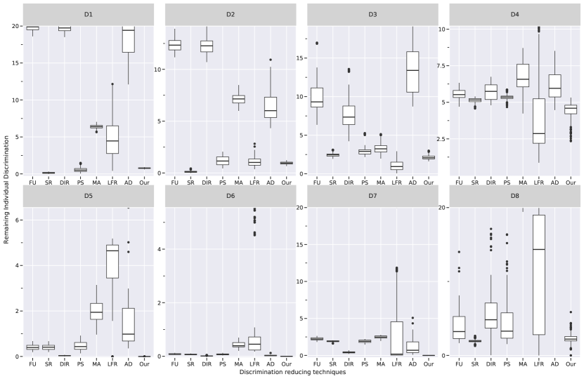
Figure 4. The individual discrimination for all 240 hyperparameter choices (lower is better). Our approach (rightmost in each boxplot) achieves low discrimination for many hyperparameter choices, and it has a little variance across choices for most datasets.

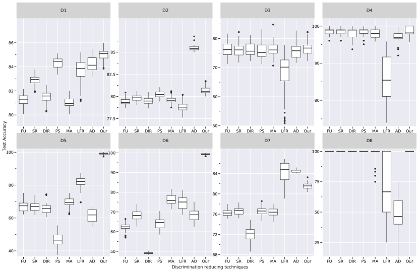
Figure 5. The test accuracy for all 240 hyperparameter choices (higher is better). Our approach is best or comparable to the best in terms of both accuracy and its variance, for all experiments except D2 and D7.

References

- (1)
- Adler et al. (2018) Philip Adler, Casey Falk, Sorelle A. Friedler, Tionney Nix, Gabriel Rybeck, Carlos Scheidegger, Brandon Smith, and Suresh Venkatasubramanian. 2018. Auditing Black-Box Models for Indirect Influence. Knowl. Inf. Syst. 54, 1 (Jan. 2018), 95–122. https://doi.org/10.1007/s10115-017-1116-3
- Agarwal et al. (2018) Alekh Agarwal, Alina Beygelzimer, Miroslav Dudik, John Langford, and Hanna Wallach. 2018. A Reductions Approach to Fair Classification. In Proceedings of Machine Learning Research, Jennifer Dy and Andreas Krause (Eds.), Vol. 80. PMLR, Stockholmsmässan, Stockholm Sweden, 60–69. http://proceedings.mlr.press/v80/agarwal18a.html
- Aggarwal et al. (2019) Aniya Aggarwal, Pranay Lohia, Seema Nagar, Kuntal Dey, and Diptikalyan Saha. 2019. Black Box Fairness Testing of Machine Learning Models. In Proceedings of the 2019 27th ACM Joint Meeting on European Software Engineering Conference and Symposium on the Foundations of Software Engineering (Tallinn, Estonia) (ESEC/FSE 2019). Association for Computing Machinery, New York, NY, USA, 625–635. https://doi.org/10.1145/3338906.3338937
- Alexandra (2018) Alexandra. 2018. 11 Ways to Reduce Hiring Bias. https://harver.com/blog/reduce-hiring-bias/. [Online; accessed 13-Septmeber-2020].
- Australia (2014) Australia. 2014. Sex Discrimination Act 1984. https://www.legislation.gov.au/Details/C2014C00002. [Online; accessed 10-September-2020].
- Barocas and Selbst (2016) Solon Barocas and Andrew D. Selbst. 2016. Big Data’s Disparate Impact. California Law Review 104 (2016), 671.
- Bechavod and Ligett (2017) Yahav Bechavod and Katrina Ligett. 2017. Learning Fair Classifiers: A Regularization-Inspired Approach. ArXiv. abs/1707.00044.
- Bellamy et al. (2018) Rachel K. E. Bellamy, Kuntal Dey, Michael Hind, Samuel C. Hoffman, Stephanie Houde, Kalapriya Kannan, Pranay Lohia, Jacquelyn Martino, Sameep Mehta, Aleksandra Mojsilovic, Seema Nagar, Karthikeyan Natesan Ramamurthy, John T. Richards, Diptikalyan Saha, Prasanna Sattigeri, Moninder Singh, Kush R. Varshney, and Yunfeng Zhang. 2018. AI Fairness 360: An Extensible Toolkit for Detecting, Understanding, and Mitigating Unwanted Algorithmic Bias. ArXiv. abs/1810.01943.
- Berk et al. (2017) R. Berk, H. Heidari, S. Jabbari, Matthew Joseph, M. Kearns, J. Morgenstern, Seth Neel, and A. Roth. 2017. A Convex Framework for Fair Regression. ArXiv. abs/1706.02409.
- Beutel et al. (2017) Alex Beutel, Jilin Chen, Zhe Zhao, and Ed Huai hsin Chi. 2017. Data Decisions and Theoretical Implications when Adversarially Learning Fair Representations. ArXiv. abs/1707.00075.
- Black et al. (2020) Emily Black, Samuel Yeom, and Matt Fredrikson. 2020. FlipTest: Fairness Testing via Optimal Transport. In Proceedings of the 2020 Conference on Fairness, Accountability, and Transparency (Barcelona, Spain) (FAT* ’20). Association for Computing Machinery, New York, NY, USA, 111–121. https://doi.org/10.1145/3351095.3372845
- Blum and Stangl (2020) Avrim Blum and Kevin Stangl. 2020. Recovering from Biased Data: Can Fairness Constraints Improve Accuracy?. In 1st Symposium on Foundations of Responsible Computing (FORC 2020) (Leibniz International Proceedings in Informatics (LIPIcs), Vol. 156). Schloss Dagstuhl–Leibniz-Zentrum für Informatik, Dagstuhl, Germany, 3:1–3:20. https://doi.org/10.4230/LIPIcs.FORC.2020.3
- Bogen et al. (2020) Miranda Bogen, Aaron Rieke, and Shazeda Ahmed. 2020. Awareness in Practice: Tensions in Access to Sensitive Attribute Data for Antidiscrimination. In Proceedings of the 2020 Conference on Fairness, Accountability, and Transparency (Barcelona, Spain) (FAT* ’20). Association for Computing Machinery, New York, NY, USA, 492–500. https://doi.org/10.1145/3351095.3372877
- Calders et al. (2009) Toon Calders, Faisal Kamiran, and Mykola Pechenizkiy. 2009. Building Classifiers with Independency Constraints. In Proceedings of the 2009 IEEE International Conference on Data Mining Workshops (ICDMW ’09). IEEE Computer Society, USA, 13–18. https://doi.org/10.1109/ICDMW.2009.83
- Calders and Verwer (2010) Toon Calders and Sicco Verwer. 2010. Three naive Bayes approaches for discrimination-free classification. Data Mining and Knowledge Discovery 21, 2 (01 Sep 2010), 277–292. https://doi.org/10.1007/s10618-010-0190-x
- Calmon et al. (2017) Flavio P. Calmon, Dennis Wei, Bhanukiran Vinzamuri, Karthikeyan Natesan Ramamurthy, and Kush R. Varshney. 2017. Optimized Pre-Processing for Discrimination Prevention. In Proceedings of the 31st International Conference on Neural Information Processing Systems (Long Beach, California, USA) (NIPS’17). Curran Associates Inc., Red Hook, NY, USA, 3995–4004.
- Card (2017) Dallas Card. 2017. The “black box” metaphor in machine learning. https://towardsdatascience.com/the-black-box-metaphor-in-machine-learning-4e57a3a1d2b0. [Online; accessed 13-April-2020].
- Card et al. (2019) Dallas Card, Michael Zhang, and Noah A. Smith. 2019. Deep Weighted Averaging Classifiers. In Proceedings of the Conference on Fairness, Accountability, and Transparency (Atlanta, GA, USA) (FAT* ’19). Association for Computing Machinery, New York, NY, USA, 369–378. https://doi.org/10.1145/3287560.3287595
- Celis et al. (2019) L. Elisa Celis, Lingxiao Huang, Vijay Keswani, and Nisheeth K. Vishnoi. 2019. Classification with Fairness Constraints: A Meta-Algorithm with Provable Guarantees. In Proceedings of the Conference on Fairness, Accountability, and Transparency (Atlanta, GA, USA) (FAT* ’19). Association for Computing Machinery, New York, NY, USA, 319–328. https://doi.org/10.1145/3287560.3287586
- Chouldechova (2017) Alexandra Chouldechova. 2017. Fair prediction with disparate impact: A study of bias in recidivism prediction instruments. Big data 5 (June 2017), 153–163.
- Corbett-Davies et al. (2017) Sam Corbett-Davies, Emma Pierson, Avi Feller, Sharad Goel, and Aziz Huq. 2017. Algorithmic Decision Making and the Cost of Fairness. In Proceedings of the 23rd ACM SIGKDD International Conference on Knowledge Discovery and Data Mining (Halifax, NS, Canada) (KDD ’17). Association for Computing Machinery, New York, NY, USA, 797–806. https://doi.org/10.1145/3097983.3098095
- Coston et al. (2020) Amanda Coston, Alan Mishler, Edward H. Kennedy, and Alexandra Chouldechova. 2020. Counterfactual Risk Assessments, Evaluation, and Fairness. In Proceedings of the 2020 Conference on Fairness, Accountability, and Transparency (Barcelona, Spain) (FAT* ’20). Association for Computing Machinery, New York, NY, USA, 582–593. https://doi.org/10.1145/3351095.3372851
- Crosman (2018) Penny Crosman. 2018. Weren’t algorithms supposed to make digital mortgages colorblind? https://www.americanbanker.com/news/werent-algorithms-supposed-to-make-digital-mortgages-colorblind. [Online; accessed 13-April-2020].
- Dastin (2018) Jeffrey Dastin. 2018. Amazon scraps secret AI recruiting tool that showed bias against women. https://www.reuters.com/misc/us-amazon-com-jobs-automation-insight/amazon-scraps-secret-ai-recruiting-tool-that-showed-bias-against-women-idUSKCN1MK08G. [Online; accessed 13-April-2020].
- Dent (2019) Kyle Dent. 2019. The risks of amoral AI. https://techcrunch.com/2019/08/25/the-risks-of-amoral-a-i/. [Online; accessed 13-Septmeber-2020].
- Didur (2018) Konstantin Didur. 2018. 12 Use Cases of AI and Machine Learning In Finance. https://towardsdatascience.com/machine-learning-in-finance-why-what-how-d524a2357b56. [Online; accessed 13-Septmeber-2020].
- Donini et al. (2018) Michele Donini, Luca Oneto, Shai Ben-David, John Shawe-Taylor, and Massimiliano Pontil. 2018. Empirical Risk Minimization under Fairness Constraints. In Proceedings of the 32nd International Conference on Neural Information Processing Systems (Montréal, Canada) (NIPS’18). Curran Associates Inc., Red Hook, NY, USA, 2796–2806.
- Dua and Graff (2017a) Dheeru Dua and Casey Graff. 2017a. UCI Machine Learning Repository - Adult Income. http://archive.ics.uci.edu/ml/datasets/Adult
- Dua and Graff (2017b) Dheeru Dua and Casey Graff. 2017b. UCI Machine Learning Repository - Default Prediction. http://archive.ics.uci.edu/ml/datasets/default+of+credit+card+clients
- Dua and Graff (2017c) Dheeru Dua and Casey Graff. 2017c. UCI Machine Learning Repository - German Credit. http://archive.ics.uci.edu/ml/datasets/statlog+(german+credit+data)
- Dua and Graff (2017d) Dheeru Dua and Casey Graff. 2017d. UCI Machine Learning Repository - Student Performance. http://archive.ics.uci.edu/ml/datasets/Student%2BPerformance
- Dunkelau and Leuschel (2019) Jannik Dunkelau and Michael Leuschel. 2019. Fairness-Aware Machine Learning. , 60 pages.
- Dwork et al. (2012) Cynthia Dwork, Moritz Hardt, Toniann Pitassi, Omer Reingold, and Richard Zemel. 2012. Fairness through Awareness. In Proceedings of the 3rd Innovations in Theoretical Computer Science Conference (Cambridge, Massachusetts) (ITCS ’12). Association for Computing Machinery, New York, NY, USA, 214–226. https://doi.org/10.1145/2090236.2090255
- Dwork et al. (2018) Cynthia Dwork, Nicole Immorlica, Adam Tauman Kalai, and Max Leiserson. 2018. Decoupled Classifiers for Group-Fair and Efficient Machine Learning. In Proceedings of Machine Learning Research, Sorelle A. Friedler and Christo Wilson (Eds.), Vol. 81. PMLR, New York, NY, USA, 119–133. http://proceedings.mlr.press/v81/dwork18a.html
- Edwards and Storkey (2015) Harrison A Edwards and Amos J. Storkey. 2015. Censoring Representations with an Adversary. CoRR. abs/1511.05897.
- Feldman et al. (2015) Michael Feldman, Sorelle A. Friedler, John Moeller, Carlos Scheidegger, and Suresh Venkatasubramanian. 2015. Certifying and Removing Disparate Impact. In Proceedings of the 21th ACM SIGKDD International Conference on Knowledge Discovery and Data Mining (Sydney, NSW, Australia) (KDD ’15). Association for Computing Machinery, New York, NY, USA, 259–268. https://doi.org/10.1145/2783258.2783311
- Fish et al. (2016) Benjamin Fish, Jeremy Kun, and Ádám Dániel Lelkes. 2016. A Confidence-Based Approach for Balancing Fairness and Accuracy. In Proceedings of the 2016 SIAM International Conference on Data Mining. Society for Industrial and Applied Mathematics, 3600 University City Science Center Philadelphia, PA, United States, 144–152. https://doi.org/10.1137/1.9781611974348.17
- Friedler et al. (2019) Sorelle A. Friedler, Carlos Scheidegger, Suresh Venkatasubramanian, Sonam Choudhary, Evan P. Hamilton, and Derek Roth. 2019. A Comparative Study of Fairness-Enhancing Interventions in Machine Learning. In Proceedings of the Conference on Fairness, Accountability, and Transparency (Atlanta, GA, USA) (FAT* ’19). Association for Computing Machinery, New York, NY, USA, 329–338. https://doi.org/10.1145/3287560.3287589
- Galhotra et al. (2017) Sainyam Galhotra, Yuriy Brun, and Alexandra Meliou. 2017. Fairness Testing: Testing Software for Discrimination. In Proceedings of the 2017 11th Joint Meeting on Foundations of Software Engineering (Paderborn, Germany) (ESEC/FSE 2017). Association for Computing Machinery, New York, NY, USA, 498–510. https://doi.org/10.1145/3106237.3106277
- Geiger et al. (2020) R. Stuart Geiger, Kevin Yu, Yanlai Yang, Mindy Dai, Jie Qiu, Rebekah Tang, and Jenny Huang. 2020. Garbage in, Garbage out? Do Machine Learning Application Papers in Social Computing Report Where Human-Labeled Training Data Comes From?. In Proceedings of the 2020 Conference on Fairness, Accountability, and Transparency (Barcelona, Spain) (FAT* ’20). Association for Computing Machinery, New York, NY, USA, 325–336. https://doi.org/10.1145/3351095.3372862
- Goel et al. (2016) Sharad Goel, Justin M. Rao, and Ravi Shroff. 2016. Precinct or prejudice? Understanding racial disparities in New York City’s stop-and-frisk policy. The Annals of Applied Statistics 10, 1 (2016), 365–394. http://www.jstor.org/stable/43826483
- Greenwood (2020) Shannon Greenwood. 2020. It’ll Be Hard To Get Approved For A Mortgage If You’re Black. https://thinkprogress.org/itll-be-hard-to-get-approved-for-a-mortgage-if-you-re-black-43634b642bdf/. [Online; accessed 13-April-2020].
- Hacker and Wiedemann (2017) Philipp Hacker and Emil Wiedemann. 2017. A continuous framework for fairness. ArXiv (2017). abs/1712.07924.
- Hajian and Domingo-Ferrer (2013) Sara Hajian and Josep Domingo-Ferrer. 2013. Direct and Indirect Discrimination Prevention Methods. In Discrimination and Privacy in the Information Society: Data Mining and Profiling in Large Databases. Springer Berlin Heidelberg, Berlin, Heidelberg, 241–254. https://doi.org/10.1007/978-3-642-30487-3_13
- Hajian et al. (2011) Sara Hajian, Josep Domingo-Ferrer, and Antoni Martínez-Ballesté. 2011. Rule Protection for Indirect Discrimination Prevention in Data Mining. In Proceedings of the 8th International Conference on Modeling Decisions for Artificial Intelligence (Changsha, China) (MDAI’11). Springer-Verlag, Berlin, Heidelberg, 211–222.
- Hamilton (2019) Ernest Hamilton. 2019. AI Perpetuating Human Bias In The Lending Space. https://www.techtimes.com/articles/240769/20190402/ai-perpetuating-human-bias-in-the-lending-space. [Online; accessed 13-April-2020].
- Hardt et al. (2016) Moritz Hardt, Eric Price, and Nathan Srebro. 2016. Equality of Opportunity in Supervised Learning. In Proceedings of the 30th International Conference on Neural Information Processing Systems (Barcelona, Spain) (NIPS’16). Curran Associates Inc., Red Hook, NY, USA, 3323–3331.
- Hu and Chen (2020) Lily Hu and Yiling Chen. 2020. Fair Classification and Social Welfare. In Proceedings of the 2020 Conference on Fairness, Accountability, and Transparency (Barcelona, Spain) (FAT* ’20). Association for Computing Machinery, New York, NY, USA, 535–545. https://doi.org/10.1145/3351095.3372857
- Hu and Kohler-Hausmann (2020) Lily Hu and Issa Kohler-Hausmann. 2020. What’s Sex Got to Do with Machine Learning?. In Proceedings of the 2020 Conference on Fairness, Accountability, and Transparency (Barcelona, Spain) (FAT* ’20). Association for Computing Machinery, New York, NY, USA, 513. https://doi.org/10.1145/3351095.3375674
- Jeff Larson and Angwin (2016) Lauren Kirchner Jeff Larson, Surya Mattu and Julia Angwin. 2016. UCI Machine Learning Repository. https://www.propublica.org/datastore/dataset/compas-recidivism-risk-score-data-and-analysis
- Johndrow and Lum (2019) James E. Johndrow and Kristian Lum. 2019. An algorithm for removing sensitive information: Application to race-independent recidivism prediction. Ann. Appl. Stat. 13, 1 (03 2019), 189–220. https://doi.org/10.1214/18-AOAS1201
- Jolly-Ryan (2012) Jennifer Jolly-Ryan. 2012. Have a Job to Get a Job: Disparate Treatment and Disparate Impact of the ’Currently Employed’ Requirement. Michigan Journal of Race and Law 18 (2012), 25. https://repository.law.umich.edu/mjrl/vol18/iss1/4
- Julia Angwin and Kirchner (2016) Surya Mattu Julia Angwin, Jeff Larson and Lauren Kirchner. 2016. Machine Bias. https://www.propublica.org/article/machine-bias-risk-assessments-in-criminal-sentencing. [Online; accessed 13-April-2020].
- Jung et al. (2019) Christopher Jung, Michael Kearns, Seth Neel, Aaron Roth, Logan Stapleton, and Zhiwei Steven Wu. 2019. Eliciting and Enforcing Subjective Individual Fairness. ArXiv. abs/1905.10660.
- Kallus et al. (2020) Nathan Kallus, Xiaojie Mao, and Angela Zhou. 2020. Assessing Algorithmic Fairness with Unobserved Protected Class Using Data Combination. In Proceedings of the 2020 Conference on Fairness, Accountability, and Transparency (Barcelona, Spain) (FAT* ’20). Association for Computing Machinery, New York, NY, USA, 110. https://doi.org/10.1145/3351095.3373154
- Kamiran and Calders (2009) Faisal Kamiran and Toon Calders. 2009. Classifying without discriminating. In 2009 2nd International Conference on Computer, Control and Communication. IEEE Computer Society, USA, 6.
- Kamiran and Calders (2010) Faisal Kamiran and Toon Calders. 2010. Classification with no discrimination by preferential sampling. In Informal proceedings of the 19th Annual Machine Learning Conference of Belgium and The Netherlands (Benelearn’10, Leuven, Belgium, May 27-28, 2010). 6.
- Kamiran and Calders (2012) Faisal Kamiran and Toon Calders. 2012. Data preprocessing techniques for classification without discrimination. Knowledge and Information Systems 33, 1 (01 Oct 2012), 1–33. https://doi.org/10.1007/s10115-011-0463-8
- Kamiran et al. (2010) Faisal Kamiran, Toon Calders, and Mykola Pechenizkiy. 2010. Discrimination Aware Decision Tree Learning. In Proceedings of the 2010 IEEE International Conference on Data Mining (ICDM ’10). IEEE Computer Society, USA, 869–874. https://doi.org/10.1109/ICDM.2010.50
- Kamiran et al. (2012) Faisal Kamiran, Asim Karim, and Xiangliang Zhang. 2012. Decision Theory for Discrimination-Aware Classification. In Proceedings of the 2012 IEEE 12th International Conference on Data Mining (ICDM ’12). IEEE Computer Society, USA, 924–929. https://doi.org/10.1109/ICDM.2012.45
- Kamishima et al. (2012) Toshihiro Kamishima, Shotaro Akaho, Hideki Asoh, and Jun Sakuma. 2012. Fairness-Aware Classifier with Prejudice Remover Regularizer. In Proceedings of the 2012th European Conference on Machine Learning and Knowledge Discovery in Databases - Volume Part II (Bristol, UK) (ECMLPKDD’12). Springer-Verlag, Berlin, Heidelberg, 35–50.
- Kamishima et al. (2011) Toshihiro Kamishima, Shotaro Akaho, and Jun Sakuma. 2011. Fairness-Aware Learning through Regularization Approach. In Proceedings of the 2011 IEEE 11th International Conference on Data Mining Workshops (ICDMW ’11). IEEE Computer Society, USA, 643–650. https://doi.org/10.1109/ICDMW.2011.83
- Kaplan and Hardy (2020) Joshua Kaplan and Benjamin Hardy. 2020. Early Data Shows Black People Are Being Disproportionally Arrested for Social Distancing Violations. https://www.propublica.org/article/in-some-of-ohios-most-populous-areas-black-people-were-at-least-4-times-as-likely-to-be-charged-with-stay-at-home-violations-as-whites. [Online; accessed 13-April-2020].
- Kilbertus et al. (2018) Niki Kilbertus, Adria Gascon, Matt Kusner, Michael Veale, Krishna Gummadi, and Adrian Weller. 2018. Blind Justice: Fairness with Encrypted Sensitive Attributes. In Proceedings of Machine Learning Research, Jennifer Dy and Andreas Krause (Eds.), Vol. 80. PMLR, Stockholmsmässan, Stockholm Sweden, 2630–2639. http://proceedings.mlr.press/v80/kilbertus18a.html
- Kilbertus et al. (2017) Niki Kilbertus, Mateo Rojas-Carulla, Giambattista Parascandolo, Moritz Hardt, Dominik Janzing, and Bernhard Schölkopf. 2017. Avoiding Discrimination through Causal Reasoning. In Proceedings of the 31st International Conference on Neural Information Processing Systems (NIPS’17). Curran Associates Inc., Long Beach, California, USA, 656–666.
- Kleinberg et al. (2016) Jon M. Kleinberg, Sendhil Mullainathan, and Manish Raghavan. 2016. Inherent Trade-Offs in the Fair Determination of Risk Scores. ArXiv.
- Kleinman (2017) Gabe Kleinman. 2017. Down With Bias, Up With Profitability. https://worldpositive.com/down-with-bias-up-with-profitability-b221e7fee0ad. [Online; accessed 13-Septmeber-2020].
- Koh and Liang (2017) Pang Wei Koh and Percy Liang. 2017. Understanding Black-Box Predictions via Influence Functions. In Proceedings of the 34th International Conference on Machine Learning - Volume 70 (ICML’17). JMLR.org, Sydney, NSW, Australia, 1885–1894.
- Kopf (2019) Dan Kopf. 2019. Goldman Sachs’ misguided World Cup predictions could provide clues to the Apple Card controversy. https://qz.com/1748321/the-role-of-goldman-sachs-algorithms-in-the-apple-credit-card-scandal/. [Online; accessed 13-Septmeber-2020].
- Kusner et al. (2017) Matt Kusner, Joshua Loftus, Chris Russell, and Ricardo Silva. 2017. Counterfactual Fairness. In Proceedings of the 31st International Conference on Neural Information Processing Systems (Long Beach, California, USA) (NIPS’17). Curran Associates Inc., Red Hook, NY, USA, 4069–4079.
- Lahoti et al. (2019) Preethi Lahoti, Krishna P. Gummadi, and Gerhard Weikum. 2019. Operationalizing Individual Fairness with Pairwise Fair Representations. Proc. VLDB Endow. 13, 4 (Dec. 2019), 506–518. https://doi.org/10.14778/3372716.3372723
- Leben (2020) Derek Leben. 2020. Normative Principles for Evaluating Fairness in Machine Learning. In Proceedings of the AAAI/ACM Conference on AI, Ethics, and Society (New York, NY, USA) (AIES ’20). Association for Computing Machinery, New York, NY, USA, 86–92. https://doi.org/10.1145/3375627.3375808
- Li et al. (2014) Yujia Li, Kevin Swersky, and Richard S. Zemel. 2014. Learning unbiased features. ArXiv. abs/1412.5244.
- Lipton et al. (2018) Zachary C. Lipton, Alexandra Chouldechova, and Julian McAuley. 2018. Does Mitigating ML’s Impact Disparity Require Treatment Disparity?. In Proceedings of the 32nd International Conference on Neural Information Processing Systems (NIPS’18). Curran Associates Inc., Montréal, Canada, 8136–8146.
- Louizos et al. (2016) Christos Louizos, Kevin Swersky, Yujia Li, Max Welling, and Richard S. Zemel. 2016. The Variational Fair Autoencoder, In ICLR. CoRR, 11. http://arxiv.org/abs/1511.00830 abs/1511.00830.
- Lum and Johndrow (2016) Kristian Lum and James E. Johndrow. 2016. A statistical framework for fair predictive algorithms. ArXiv. abs/1610.08077.
- Luong et al. (2011) Binh Thanh Luong, Salvatore Ruggieri, and Franco Turini. 2011. K-NN as an Implementation of Situation Testing for Discrimination Discovery and Prevention. In Proceedings of the 17th ACM SIGKDD International Conference on Knowledge Discovery and Data Mining (San Diego, California, USA) (KDD ’11). Association for Computing Machinery, New York, NY, USA, 502–510. https://doi.org/10.1145/2020408.2020488
- Madhavan and Wadhwa (2020) Ramanujam Madhavan and Mohit Wadhwa. 2020. Fairness-Aware Learning with Prejudice Free Representations. ArXiv. abs/2002.12143.
- Madras et al. (2019) David Madras, Elliot Creager, Toniann Pitassi, and Richard Zemel. 2019. Fairness through Causal Awareness: Learning Causal Latent-Variable Models for Biased Data. In Proceedings of the Conference on Fairness, Accountability, and Transparency (Atlanta, GA, USA) (FAT* ’19). Association for Computing Machinery, New York, NY, USA, 349–358. https://doi.org/10.1145/3287560.3287564
- Martin (2018) Nicole Martin. 2018. Are AI Hiring Programs Eliminating Bias Or Making It Worse? https://www.forbes.com/sites/nicolemartin1/2018/12/13/are-ai-hiring-programs-eliminating-bias-or-making-it-worse/. [Online; accessed 13-April-2020].
- McNamara et al. (2017) Daniel McNamara, Cheng Soon Ong, and Robert C. Williamson. 2017. Provably Fair Representations. ArXiv. abs/1710.04394.
- Mehrabi et al. (2019) Ninareh Mehrabi, Fred Morstatter, Nripsuta Saxena, Kristina Lerman, and Aram Galstyan. 2019. A Survey on Bias and Fairness in Machine Learning. arXiv:1908.09635 [cs]. http://arxiv.org/abs/1908.09635
- Menon and Williamson (2018) Aditya Krishna Menon and Robert C Williamson. 2018. The cost of fairness in binary classification. In Proceedings of Machine Learning Research, Vol. 81. PMLR, New York, NY, USA, 107–118. http://proceedings.mlr.press/v81/menon18a.html
- Metevier et al. (2019) Blossom Metevier, Stephen Giguere, Sarah Brockman, Ari Kobren, Yuriy Brun, Emma Brunskill, and Philip S. Thomas. 2019. Offline Contextual Bandits with High Probability Fairness Guarantees. In Advances in Neural Information Processing Systems 32. Curran Associates, Inc., Red Hook, NY, USA, 14922–14933. http://papers.nips.cc/paper/9630-offline-contextual-bandits-with-high-probability-fairness-guarantees.pdf
- Nabi and Shpitser (2018) Razieh Nabi and Ilya Shpitser. 2018. Fair Inference on Outcomes. In Proceedings of the Thirty-Second AAAI Conference on Artificial Intelligence. AAAI Press, New Orleans, Louisiana, USA, 1931–1940. https://www.aaai.org/ocs/index.php/AAAI/AAAI18/paper/view/16683
- Ncasas (2017) Ncasas. 2017. Why are Machine Learning models called black boxes? https://datascience.stackexchange.com/questions/22335/why-are-machine-learning-models-called-black-boxes. [Online; accessed 13-April-2020].
- Pearl (2009) Judea Pearl. 2009. Causality: Models, Reasoning and Inference (2nd ed.). Cambridge University Press, USA.
- Pedreschi et al. (2009) Dino Pedreschi, Salvatore Ruggieri, and Franco Turini. 2009. Measuring Discrimination in Socially-Sensitive Decision Records. In Proceedings of the 2009 SIAM International Conference on Data Mining. Society for Industrial and Applied Mathematics, 3600 University City Science Center Philadelphia, PA, United States, 581–592. https://doi.org/10.1137/1.9781611972795.50
- Pedreshi et al. (2008) Dino Pedreshi, Salvatore Ruggieri, and Franco Turini. 2008. Discrimination-Aware Data Mining. In Proceedings of the 14th ACM SIGKDD International Conference on Knowledge Discovery and Data Mining (Las Vegas, Nevada, USA) (KDD ’08). Association for Computing Machinery, New York, NY, USA, 560–568. https://doi.org/10.1145/1401890.1401959
- Pleiss et al. (2017) Geoff Pleiss, Manish Raghavan, Felix Wu, Jon Kleinberg, and Kilian Q. Weinberger. 2017. On Fairness and Calibration. In Proceedings of the 31st International Conference on Neural Information Processing Systems (Long Beach, California, USA) (NIPS’17). Curran Associates Inc., Red Hook, NY, USA, 5684–5693.
- PODESTA (2014) JOHN PODESTA. 2014. BIG DATA: SEIZING OPPORTUNITIES, PRESERVING VALUES. https://perma.cc/ZXB4-SDL9. [Online; accessed 13-Septmeber-2020].
- Pope and Sydnor (2011) Devin G. Pope and Justin R. Sydnor. 2011. Implementing Anti-Discrimination Policies in Statistical Profiling Models. American Economic Journal: Economic Policy 3, 3 (2011), 206–231. http://www.jstor.org/stable/41238108
- Resnick (2019) Brian Resnick. 2019. Yes, artificial intelligence can be racist. https://www.vox.com/science-and-health/2019/1/23/18194717/alexandria-ocasio-cortez-ai-bias. [Online; accessed 13-Septmeber-2020].
- Rodriguez (2020) German Rodriguez. 2020. Discrimination in Salaries. https://data.princeton.edu/wws509/datasets/#salary. [Online; accessed 13-April-2020].
- Ruoss et al. (2020) Anian Ruoss, Mislav Balunovic, Marc Fischer, and Martin T. Vechev. 2020. Learning Certified Individually Fair Representations. ArXiv. abs/2002.10312.
- Russell et al. (2017a) Chris Russell, Matt J Kusner, Joshua Loftus, and Ricardo Silva. 2017a. When Worlds Collide: Integrating Different Counterfactual Assumptions in Fairness. In Advances in Neural Information Processing Systems 30, I. Guyon, U. V. Luxburg, S. Bengio, H. Wallach, R. Fergus, S. Vishwanathan, and R. Garnett (Eds.). Curran Associates, Inc., Red Hook, NY, USA, 6414–6423. http://papers.nips.cc/paper/7220-when-worlds-collide-integrating-different-counterfactual-assumptions-in-fairness.pdf
- Russell et al. (2017b) Chris Russell, Matt J. Kusner, Joshua R. Loftus, and Ricardo Silva. 2017b. When Worlds Collide: Integrating Different Counterfactual Assumptions in Fairness. In Proceedings of the 31st International Conference on Neural Information Processing Systems (Long Beach, California, USA) (NIPS’17). Curran Associates Inc., Red Hook, NY, USA, 6417–6426.
- Salimi et al. (2019) Babak Salimi, Luke Rodriguez, Bill Howe, and Dan Suciu. 2019. Interventional Fairness: Causal Database Repair for Algorithmic Fairness. In Proceedings of the 2019 International Conference on Management of Data (Amsterdam, Netherlands) (SIGMOD ’19). Association for Computing Machinery, New York, NY, USA, 793–810. https://doi.org/10.1145/3299869.3319901
- Selbst (2017) Andrew D. Selbst. 2017. Disparate Impact in Big Data Policing. Georgia law review 52 (2017), 3373.
- Sharifi-Malvajerdi et al. (2019) Saeed Sharifi-Malvajerdi, Michael Kearns, and Aaron Roth. 2019. Average Individual Fairness: Algorithms, Generalization and Experiments. In Advances in Neural Information Processing Systems 32. Curran Associates, Inc., Red Hook, NY, USA, 8242–8251. http://papers.nips.cc/paper/9034-average-individual-fairness-algorithms-generalization-and-experiments.pdf
- Simoiu et al. (2017) Camelia Simoiu, Sam Corbett-Davies, and Sharad Goel. 2017. The problem of infra-marginality in outcome tests for discrimination. Annals of Applied Statistics 11, 3 (09 2017), 1193–1216. https://doi.org/10.1214/17-AOAS1058
- Skeem and Lowenkamp (2016) Jennifer Lynne Skeem and Christopher T. Lowenkamp. 2016. RISK, RACE, AND RECIDIVISM: PREDICTIVE BIAS AND DISPARATE IMPACT*: RISK, RACE, AND RECIDIVISM. Criminology 54 (2016), 680–712.
- Steil et al. (2017) Justin Steil, Len Albright, Jacob Rugh, and Douglas Massey. 2017. The Social Structure of Mortgage Discrimination. Housing Studies 33 (11 2017), 1–18. https://doi.org/10.1080/02673037.2017.1390076
- Techlabs (2020) Maruti Techlabs. 2020. 12 Use Cases of AI and Machine Learning In Finance. https://marutitech.com/ai-and-ml-in-finance/. [Online; accessed 13-Septmeber-2020].
- Thomas et al. (2019) Philip S. Thomas, Bruno Castro da Silva, Andrew G. Barto, Stephen Giguere, Yuriy Brun, and Emma Brunskill. 2019. Preventing undesirable behavior of intelligent machines. Science 366, 6468 (2019), 999–1004. https://doi.org/10.1126/science.aag3311 arXiv:https://science.sciencemag.org/content/366/6468/999.full.pdf
- Ting (2017) Kai Ming Ting. 2017. Confusion Matrix. Springer US, Boston, MA, 260–260. https://doi.org/10.1007/978-1-4899-7687-1_50
- Udeshi et al. (2018) Sakshi Udeshi, Pryanshu Arora, and Sudipta Chattopadhyay. 2018. Automated Directed Fairness Testing. In Proceedings of the 33rd ACM/IEEE International Conference on Automated Software Engineering (Montpellier, France) (ASE 2018). Association for Computing Machinery, New York, NY, USA, 98–108. https://doi.org/10.1145/3238147.3238165
- Veale and Binns (2017a) Michael Veale and Reuben Binns. 2017a. Fairer machine learning in the real world: Mitigating discrimination without collecting sensitive data. Big Data & Society 4, 2 (2017), 2053951717743530. https://doi.org/10.1177/2053951717743530
- Veale and Binns (2017b) Michael Veale and Reuben Binns. 2017b. Fairer machine learning in the real world: Mitigating discrimination without collecting sensitive data. Big Data & Society 4 (2017), 17.
- Verma and Rubin (2018) Sahil Verma and Julia Rubin. 2018. Fairness definitions explained. In Proceedings of the International Workshop on Software Fairness - FairWare ’18. ACM Press, Gothenburg, Sweden, 1–7. https://doi.org/10.1145/3194770.3194776
- Žliobaite and Custers (2016) Indre; Žliobaite and Bart Custers. 2016. Using Sensitive Personal Data May Be Necessary for Avoiding Discrimination in Data-Driven Decision Models. Artif. Intell. Law 24, 2 (June 2016), 183–201. https://doi.org/10.1007/s10506-016-9182-5
- Wadsworth et al. (2018) Christina Wadsworth, Francesca Vera, and Chris Piech. 2018. Achieving Fairness through Adversarial Learning: an Application to Recidivism Prediction. arXiv:1807.00199 [cs, stat]. , 5 pages. http://arxiv.org/abs/1807.00199 arXiv: 1807.00199.
- Wick et al. (2019) Michael Wick, swetasudha panda, and Jean-Baptiste Tristan. 2019. Unlocking Fairness: a Trade-off Revisited. In Advances in Neural Information Processing Systems 32. Curran Associates, Inc., Red Hook, NY, USA, 8783–8792. http://papers.nips.cc/paper/9082-unlocking-fairness-a-trade-off-revisited.pdf
- Wieringa (2020) Maranke Wieringa. 2020. What to Account for When Accounting for Algorithms: A Systematic Literature Review on Algorithmic Accountability. In Proceedings of the 2020 Conference on Fairness, Accountability, and Transparency (Barcelona, Spain) (FAT* ’20). Association for Computing Machinery, New York, NY, USA, 1–18. https://doi.org/10.1145/3351095.3372833
- Wikipedia contributors (2020) Wikipedia contributors. 2020. Redlining — Wikipedia, The Free Encyclopedia. https://en.wikipedia.org/w/index.php?title=Redlining. [Online; accessed 13-April-2020].
- Williams et al. (2018a) Betsy Anne Williams, Catherine F. Brooks, and Yotam Shmargad. 2018a. How Algorithms Discriminate Based on Data They Lack: Challenges, Solutions, and Policy Implications. Journal of Information Policy 8 (2018), 78–115. https://www.jstor.org/stable/10.5325/jinfopoli.8.2018.0078
- Williams et al. (2018b) Betsy Anne Williams, Catherine F. Brooks, and Yotam Shmargad. 2018b. How Algorithms Discriminate Based on Data They Lack: Challenges, Solutions, and Policy Implications. Journal of Information Policy 8 (2018), 78–115.
- Winrow and Schieber (2010) Brian P. Winrow and Christen Schieber. 2010. The Disparity between Disparate Treatment and Disparate Impact: An Analysis of the Ricci Case, In Journal of Legal, Ethical and Regulatory Issues. The DreamCatchers Group, LLC 13, 14.
- Woodworth et al. (2017) Blake Woodworth, Suriya Gunasekar, Mesrob I. Ohannessian, and Nathan Srebro. 2017. Learning Non-Discriminatory Predictors. In Proceedings of Machine Learning Research, Vol. 65. PMLR, Amsterdam, Netherlands, 1920–1953. http://proceedings.mlr.press/v65/woodworth17a.html
- Yang et al. (2020) Kaiyu Yang, Klint Qinami, Li Fei-Fei, Jia Deng, and Olga Russakovsky. 2020. Towards Fairer Datasets: Filtering and Balancing the Distribution of the People Subtree in the ImageNet Hierarchy. In Proceedings of the 2020 Conference on Fairness, Accountability, and Transparency (Barcelona, Spain) (FAT* ’20). Association for Computing Machinery, New York, NY, USA, 547–558. https://doi.org/10.1145/3351095.3375709
- Zafar et al. (2017a) Muhammad Bilal Zafar, Isabel Valera, Manuel Gomez Rodriguez, and Krishna P. Gummadi. 2017a. Fairness Beyond Disparate Treatment & Disparate Impact: Learning Classification without Disparate Mistreatment. In Proceedings of the 26th International Conference on World Wide Web (Perth, Australia) (WWW ’17). International World Wide Web Conferences Steering Committee, Republic and Canton of Geneva, CHE, 1171–1180. https://doi.org/10.1145/3038912.3052660
- Zafar et al. (2017b) Muhammad Bilal Zafar, Isabel Valera, Manuel Gomez-Rodriguez, and Krishna P. Gummadi. 2017b. Fairness Constraints: Mechanisms for Fair Classification. In Proceedings of the 20th International Conference on Artificial Intelligence and Statistics, AISTATS (Proceedings of Machine Learning Research, Vol. 54). PMLR, Fort Lauderdale, FL, USA, 962–970. http://proceedings.mlr.press/v54/zafar17a.html
- Zemel et al. (2013) Richard Zemel, Yu Wu, Kevin Swersky, Toniann Pitassi, and Cynthia Dwork. 2013. Learning Fair Representations. In Proceedings of the 30th International Conference on International Conference on Machine Learning - Volume 28 (ICML’13). JMLR.org, Atlanta, GA, USA, III–325–III–333.
- Zhang et al. (2018) Brian Hu Zhang, Blake Lemoine, and Margaret Mitchell. 2018. Mitigating Unwanted Biases with Adversarial Learning. In Proceedings of the 2018 AAAI/ACM Conference on AI, Ethics, and Society (New Orleans, LA, USA) (AIES ’18). Association for Computing Machinery, New York, NY, USA, 335–340. https://doi.org/10.1145/3278721.3278779