Nuclear Zeeman Effect on Heading Errors and the Suppression in Atomic Magnetometers

Abstract

Precession frequencies measured by optically-pumped scalar magnetometers are dependent on the relative angle between the sensor and the external magnetic field, resulting in the so-called heading errors if the magnetic field orientation is not well known or is not stable. The heading error has been known to be caused mainly by the nonlinear Zeeman effect and the orientation-dependent light shift. In this work, we find that the nuclear Zeeman effect can also a significant impact on the heading errors, especially for continuously-driving magnetometers with unresolved magnetic transitions. It not only shifts the precession frequency but deforms the heading errors and causes asymmetry: the heading errors for pump lasers with opposite helicities are different. The heading error also depends on the relative direction (parallel or vertical) of the probe laser to the RF driving magnetic field. Thus, one can design the configuration of the magnetometer and make it work in the smaller-heading-error regime. To suppress the heading error, our studies suggest to sum up the output precession frequencies from atomic cells pumped by two lasers with opposite helicities and probed by lasers propagating in orthogonal directions (one parallel and another perpendicular to the RF field), instead of utilizing probe lasers propagating in the same directions. Due to the nuclear Zeeman effect, the average precession frequencies in the latter case can have a non-negligible angular dependence, while in the former case the nuclear-Zeeman-effect induced heading error can be largely compensated and the residue is within $1$Hz. Furthermore, for practical use, we propose to simply utilize a small magnetic field parallel/antiparallel to the pump laser. By tuning the magnitude of this auxiliary field, the heading error can be flattened around different angles, which can improve the accuracy when the magnetometer works around a certain orientation angle.

Optically-pumped magnetometers have achieved high sensitivity Kominis et al. (2003); Budker (2003); Budker and Romalis (2007) and have been applied in a broad range from archaeology and geophysics Kvamme (2006); Gaffney (2008); Dang and Romalis (2010); Vasilakis et al. (2009) to fundamental physics Fortson et al. (2003); Amini et al. (2007); Roberts et al. (2015). In scalar atomic magnetometers, the magnitude of the external magnetic field is determined by measuring the precession frequency of alkali-metal atoms. This frequency is dependent on the sensor’s orientation with respect to the magnetic field, resulting in the so-called heading errors Yabuzaki and Ogawa (1974); Alexandrov (2003); Ben-Kish and Romalis (2010); Bao et al. (2018), which is one of the major sources of accuracy degradation especially for magnetometers operating in the geophysical range ($20-80$ $\mu$T).

Heading errors in atomic magnetometers have been studied both theoretically and experimentally Yabuzaki and Ogawa (1974); Hovde et al. (2011); Colombo et al. (2017); Bao et al. (2018); Oelsner et al. (2019). It has been shown Oelsner et al. (2019) that the main contributions to heading errors in continuously-pumped magnetometers are the nonlinear Zeeman (NLZ) effects Seltzer et al. (2007); Bao et al. (2018); Jensen et al. (2009); Chalupczak et al. (2010) and the light shift (LS) Happer (1972); Scholtes et al. (2012); Appelt et al. (1998); Chang et al. (2019) (in continuously-driving systems) that is orientation dependent. In most of these studies, apart from a small correction to the Larmor frequency, the interaction between the external magnetic field and the nuclear spins is neglected since the nuclear magneton $\mu_{\mathrm{N}}$ is about $3$ orders smaller than the Bohr magneton $\mu_{\mathrm{B}}$. However, in the geophysical field range, the linear nuclear Zeeman (NuZ) splitting is larger than or comparable with the NLZ shift. For instance, for $\left.{}^{85}\text{Rb}\right.$ in a field $B_{0}=55\mathrm{\mu T}$, the former is about $226$Hz while the latter is about $22$Hz. When the frequencies of transitions between adjacent magnetic levels are not resolved, for instance, when the linewidth of the individual transitions is relatively large in the presence of several hundreds of buffer gas, the NuZ effect is non-negligible for the heading errors, especially for continuously-driving magnetometers. In this paper, we theoretically and experimentally study the heading error in atomic magnetometers by including the NuZ effect and find that it can significantly modify the heading errors. The setup for our study is schematically shown in Fig. 1(a), where an atomic cell containing alkali-metal atoms and buffer gas ($\mathrm{N_{2}}$) is exposed to the external magnetic field $\vec{B}_{0}=B_{0}\hat{e}_{z}$ along the $z$ direction. The circularly-polarized pump laser, whose propagation direction together with $\vec{B}_{0}$ defines the $xz$ plane, is tilted by an angle $\theta$ to $\vec{B}_{0}$. An oscillating magnetic field perpendicular to the pump laser is generated by RF coils to induce atomic spin polarizations in the $xy$ plane, which is reconstructed by measuring the optical rotation of a linearly-polarized probe laser. Without loss of generality, we assume the RF field is in the $xz$ plane and the probe laser propagates parallel or perpendicular (along the $y$ direction) to the RF field since only their relative direction matters. For parallel probe lasers, we find that, compared to the case without the NuZ effect, the heading error is smaller/larger when the pump laser is left/right-handed circularly polarized ($\sigma^{+}/\sigma^{-}$). For vertical probe lasers, however, it is another way around. This suggests to reduce the heading errors by employing two pump lasers with opposite helicities and two probe lasers with one parallel while another perpendicular to the driving field. Furthermore, for practical use, we propose a simple scheme to suppress the heading error by utilizing a small magnetic field parallel (for $\sigma^{+}$ polarization) or antiparallel (for $\sigma^{-}$ polarization) to the pump laser. By tuning the magnitude of this auxiliary field, the heading error can be flattened around different orientation angles.

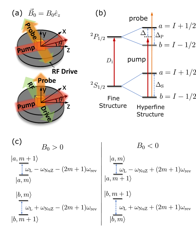
Figure 1: (a) Schematic of an atomic magnetometer fixed on a rotatable table (the gray disc). Here, an atomic cell (yellow cubic at the center) containing alkali-metal atoms and buffer gas is pumped by a circularly-polarized laser (red arrow) propagating in the $xz$ plane with a tilted angle $\theta$ to the external field $\vec{B}_{0}=B_{0}\hat{e}_{z}$. A small RF magnetic field (green double arrow) drives the atoms and the induced precession is measured by the linearly-polarized probe laser (orange arrow) propagating parallel (upper figure) or perpendicular (lower figure) to the RF field. (b) Fine states and hyperfine states of the alkali-metal atom. The pump laser induces transitions (D1 transition) between the ground states $\left|Fm\right\rangle_{S}$ and the first excited states $\left|Fm\right\rangle_{P}$ with $F=a,b$, and $m$ the magnetic number. The probe laser is far detuned from this D1 transition. (c) Energy level spacing between two adjacent ground-state Zeeman sublevels of the alkali-metal atom. Besides the Larmor frequency$\ \omega_{\mathrm{L}}\equiv\mu_{\mathrm{eff}}\left|B_{0}\right|$ and the quantum beat revival frequency $\omega_{\mathrm{rev}}\equiv\mu_{\mathrm{eff}}^{2}B_{0}^{2}/\Delta_{S}$, there is the third term $\omega_{\mathrm{NuZ}}\equiv g_{I}\mu_{\mathrm{N}}\left|B_{0}\right|$ coming from the linear NuZ splitting, leading to different precession frequencies in the $a$ and $b$ hyperfine manifolds.

It can be proved sup that the precession frequency is invariant when changing $\theta$ to$\ -\theta$, and inverting the helicity of the pump laser is equivalent to inverting its propagation direction or inverting $\vec{B}_{0}$. Therefore, in this letter, we take the $z$ axis as the quantization axis and focus on the $\sigma^{+}$-polarized pump with the pump laser’s orientation angle $\theta\in[0,\pi/2]$. For the $\sigma^{-}$-polarized pump, we only need to change $B_{0}$ to $-B_{0}$ in the calculation. For the D1 transition, in the rotating frame with respect to the pump laser’s frequency, the master equation for the alkali-metal atom is Happer et al. (2010); Appelt et al. (1998); Lancor and Walker (2010):

$$\partial_{t}\rho=-i\left[H,\rho\right]+\mathcal{L}_{PP}\rho+\mathcal{L}_{SP}\rho+\mathcal{L}_{SS}\rho.$$ (1)

Here, the Hamiltonian $H=H_{HF}+H_{B}+H_{LA}+H_{D}$, where $H_{HF}$ is the hyperfine interaction

$$H_{HF} = \sum_{m}\Delta_{S}\left|am\right\rangle_{SS}\left\langle am\right|+\Delta\left|am\right\rangle_{PP}\left\langle am\right|$$ (2)

$$+\left(\Delta-\Delta_{P}\right)\left|bm\right\rangle_{PP}\left\langle bm\right|$$

with the hyperfine splitting $\Delta_{S}$ ($\Delta_{P}$) in the ground states $\left|Fm\right\rangle_{S}$ (excited states $\left|Fm\right\rangle_{P}$), $F=a$, $b$, and the detuning $\Delta$ of the pump laser (see Fig. 1(b)); $H_{B}$ depicts the interaction between the spins and the external magnetic field

$$H_{B}=g_{e}\mu_{\mathrm{B}}B_{z}S_{z}+g_{I}\mu_{\mathrm{N}}B_{z}I_{z}$$ (3)

with the electron (nuclear) spin operator$\vec{S}$ ($\vec{I}$) and the electron (nuclear) g-factor $g_{e}$ ($g_{I}$) of the alkali-metal atom; $H_{LA}$ is the light-atom interaction

$$H_{LA}=-\frac{E_{0}}{2}\left(\frac{1}{\sqrt{2}}\sum_{\sigma=\pm 1}d_{\sigma}\left(\cos\theta+\sigma\right)+d_{z}\sin\theta\right)$$ (4)

with the electric field $E_{0}$ of the pump laser and the atom’s dipole moment $\vec{d}$ while $d_{\pm 1}\equiv-\left(d_{x}\pm id_{y}\right)/\sqrt{2}$. Note that under the rotating-wave approximation, the dipole moment $d_{\pm}$ has only matrix elements between $\left|Fm\right\rangle_{S}$ and $\left|Fm\pm 1\right\rangle_{P}$ Walls and Milburn (2008). The coupling to the driving field $H_{D}=g_{e}\mu_{\mathrm{B}}B_{1}\left(S_{x}\cos\theta-S_{z}\sin\theta\right)\cos\omega t$ induces polarization in the $xy$ plane. In experiments, the precession frequency is determined by the zero crossing $\omega_{0}$ of the in-phase part in $\left\langle S_{x}\cos\theta+S_{z}\sin\theta\right\rangle$ when the probe laser is parallel to the RF field ($\omega_{0,\parallel}$) or out-of-phase part in $\left\langle S_{y}\right\rangle$ when the probe laser is perpendicular to the RF field ($\omega_{0,\perp}$). Apart from the coherent dynamics, the alkali-metal atom experiences excited-state mixture Happer et al. (2010); Lancor and Walker (2010) ($\mathcal{L}_{PP}$) and quenching Happer et al. (2010); Lancor and Walker (2010) ($\mathcal{L}_{SP}$) caused by collisions between alkali-metal atoms in excited states and buffer gas atoms, and dissipation Happer et al. (2010); Appelt et al. (1998) ($\mathcal{L}_{SS}$)  in the ground states induced by collisions between alkali-metal atoms.

Within the geophysical range, the interaction $H_{B}$ can be treated as a perturbation to the hyperfine states. To the second, the energy $E\left(a/b,m\right)$ (apart from a constant independent of $B_{0}$) of the ground-state Zeeman sublevel $\left|a\text{/}b\text{, }m\right\rangle_{S}$ is

$$E\left(a/b,m\right)\approx\left(\pm\mu_{\mathrm{eff}}-g_{I}\mu_{\mathrm{N}}\right)B_{0}m\mp\omega_{\mathrm{rev}}m^{2},$$ (5)

where the effective magneton $\mu_{\mathrm{eff}}\equiv\left(g_{S}\mu_{\mathrm{B}}+g_{I}\mu_{\mathrm{N}}\right)/\left(2I+1\right)$ and the quantum-beat revival frequency $\omega_{\mathrm{rev}}\equiv\mu_{\mathrm{eff}}^{2}B_{0}^{2}/\Delta_{S}$. The last term in Eq. (5) is the lowest-order NLZ splitting Jensen et al. (2009); Chalupczak et al. (2010). With this NLZ effect, the energy spacing between two adjacent Zeeman sublevels depends on the magnetic quantum number $m$, as shown in Fig. 1(c), leading to heading errors: the population in each state $\left|Fm\right\rangle_{S}$ changes when orientation angle $\theta$ varies and thus the measured precession frequency $\omega_{0}$ is dependent on $\theta$. Another contribution to heading errors is the LS Oelsner et al. (2019) that shifts the energy of the state $\left|Fm\right\rangle_{S}$ by an amount depending on $m$ and $\theta$. Apart from the NLZ effect and LS, we find that the NuZ effect also causes heading errors. Fig. 1(c) shows that for the same $m$, the adjacent-states’ energy level spacings in the $a$ and $b$ manifolds are different because of the linear NuZ splitting $\omega_{\mathrm{NuZ}}\equiv g_{I}\mu_{\mathrm{N}}\left|B_{0}\right|$. As $\theta$ varies, the populations in the $a$ and $b$ manifolds change, shifting the precession frequency. Note that inverting the helicity of the pump is equivalent to inverting $\vec{B}_{0}$, so we plot the energy spacings in Fig. 1(c) for $\pm B_{0}$ to illustrate physical insights for the opposite-helicity case.

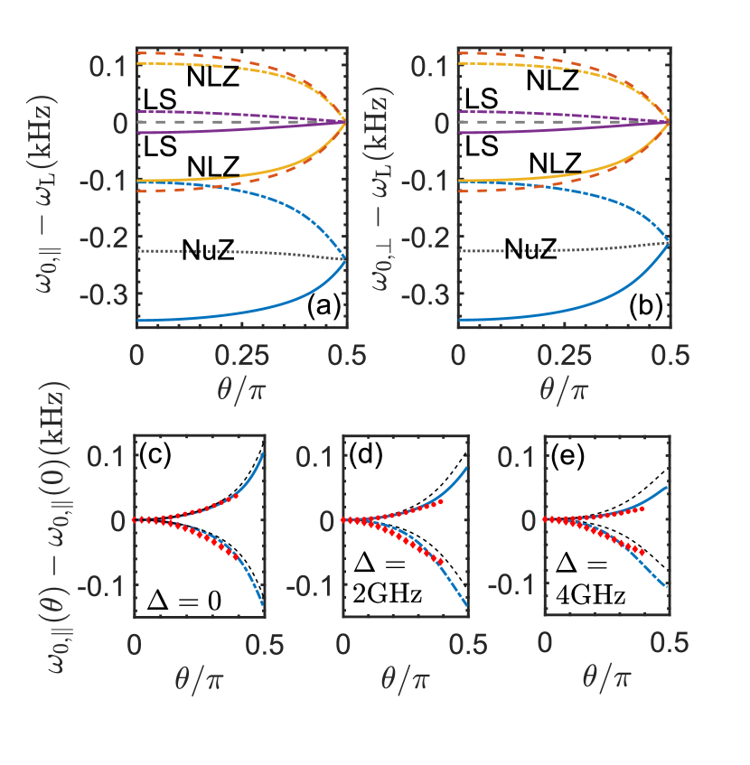
Figure 2: (a) Contributions to the precession frequency $\omega_{0}$ (shown as the deviation from the Larmor frequency $\omega_{\mathrm{L}}$) from the NLZ effect, LS, and the NuZ effect, with the probe laser parallel (a) or perpendicular (b) to the RF field. The detuning $\Delta$ of the pump laser is $0$. Here and after, if not specified, solid lines are for $\sigma^{+}$ polarization while dotted-dashed lines are for the negative $\sigma^{-}$ case. The precession frequencies when including all the three contributions are shown at the bottom as the blue lines. Their average value $\left[\omega_{0}^{+}\left(\theta\right)+\omega_{0}^{-}\left(\theta\right)\right]/2-\omega_{\mathrm{L}}$ is just the precession frequency when including only the NuZ effect (black dotted line). For comparison, the precession frequencies when neglecting the NuZ effect and its average values are shown as the red and flat grey dash lines respectively in the upper part. (c)-(e) Heading errors $\omega_{0,\parallel}\left(\theta\right)-\omega_{0,\parallel}\left(0\right)$ for different detuning $\Delta$. The results without the NuZ effect are shown as the grey dash lines, while the experimental data are plotted in dots ($\sigma^{+}$) and diamonds ($\sigma^{-}$).

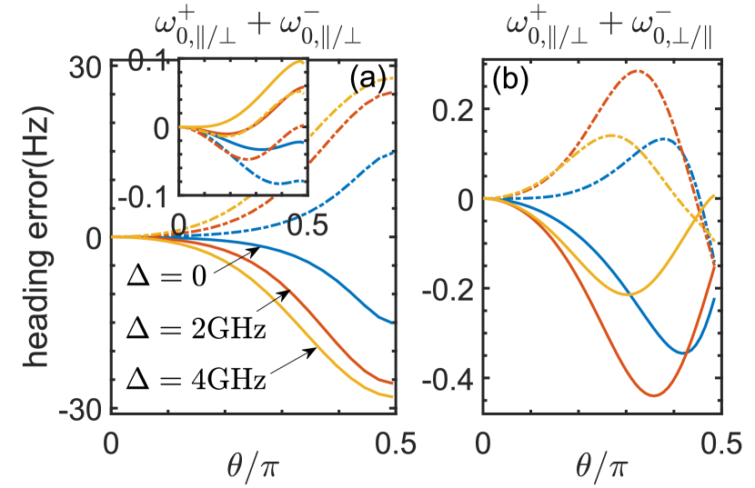
Figure 3: Heading errors in the average of two magnetometers pumped by lasers with opposite helicities. Parameters are the same as in Fig. 2. (a) Solid lines are for $\omega_{0,\parallel}^{+}+\omega_{0,\parallel}^{-}$ while dotted-dash lines are for $\omega_{0,\perp}^{+}+\omega_{0,\perp}^{-}$. The inset shows the result without the NuZ effect. (b) Solid lines are $\omega_{0,\parallel}^{+}+\omega_{0,\perp}^{-}$ while dotted dashed lines are for $\omega_{0,\perp}^{+}+\omega_{0,\parallel}^{-}$.

With the experimental condition: in a magnetic shield, a $4^{3}$mm${}^{3}\ \left.{}^{85}\text{Rb}\right.$ cell with $700$Torr N₂ is heated to $90$ Celsius, the pump laser’s power is around $50$ $\mathrm{\mu W}$, and the probe laser is about $0.2$nm detuned from the D1 transition, we solve numerically the master equation (1) by adiabatically eliminating the excited states Gardiner and Zoller (2004) and applying the linear response theory Fetter and Walecka (2012) for the RF driving Chang et al. (2019). The deviation of the precession frequency $\omega_{0,\parallel/\perp}\left(\theta\right)$ from the Larmor frequency $\omega_{\mathrm{L}}$ is plotted in Fig. 2(a) and (b) for $B_{0}=55\mathrm{\mu T}$, with the pump laser’s detuning $\Delta=0$. It shows that: (1) the precession frequency is smaller than $\omega_{\mathrm{L}}$, since in the $a$ manifold that has more population than the $b$ manifold because of the optical pumping, the linear NuZ effect contributes $-\omega_{\mathrm{NuZ}}$ to the precession frequency and this contribution is larger than the NLZ effect and LS; (2) the precession frequency $\omega_{0,\parallel/\perp}^{+}\left(\theta\right)$ for the $\sigma^{+}$ polarization is smaller than $\omega_{0,\parallel/\perp}^{-}\left(\theta\right)$ for the $\sigma^{-}$ case because of the sign of the NLZ splitting for the $m>0$ states which has more populations than the $m<0$ ones; (3) as $\theta$ increases, $\omega_{0,\parallel/\perp}^{+}\left(\theta\right)$ increases ($\omega_{0,\parallel/\perp}^{-}\left(\theta\right)$ decreases) because states with smaller $m$ and states in the $b$ manifolds get more populated and these states have lager (smaller) precession frequencies; (4) the heading errors for opposite helicity pumps are not symmetric Yabuzaki and Ogawa (1974), i.e., for two given angles $\theta_{1}$ and $\theta_{2}$,

$$\omega_{0}^{+}\left(\theta_{1}\right)-\omega_{0}^{+}\left(\theta_{2}\right)\neq\omega_{0}^{-}\left(\theta_{2}\right)-\omega_{0}^{-}\left(\theta_{1}\right),$$ (6)

which holds for both the parallel and vertical probe lasers. We note that this asymmetry was also presented Yabuzaki and Ogawa (1974). In the following, we will show that this asymmetry is resulted from the NuZ effect.

The precession frequencies from the three sources: the NLZ effect, the LS, and the NuZ are also separately shown. We see that both the NLZ effect and the LS lead to symmetric heading errors for positive and negative $B_{0}$, and they average to the Larmor frequency sym ; sup . However, the precession frequency results in the same precession frequencies for both the $\sigma^{\pm}$-polarization cases sup , which is just the angular dependence of the average value $\left(\omega_{0}^{+}+\omega_{0}^{-}\right)/2-\omega_{\mathrm{L}}$ when including all three effects, and results in smaller heading error for $\sigma^{+}$ polarization with parallel probe lasers but larger with vertical probe lasers.

The total heading error $\omega_{0,\parallel}\left(\theta\right)-\omega_{0,,\parallel}\left(0\right)$ with the parallel probe laser is shown in Fig. 2(c)-(e) for different detunings $\Delta=0$, $2\mathrm{GHz}$, and $4\mathrm{GHz}$, respectively. For comparison, the results without the NuZ effect are also plotted. When $\Delta=0$, the $b$-manifold is resonantly pumped and its population is small. Therefore, the NuZ effect is not significant. However, when $\Delta$ increases and more populations are in the $b$-manifold, the heading errors with and without the NuZ effect deviate a lot, and the experimental data agrees with the former one exp .

Considering the heading-error asymmetry that is shown to be induced by the NuZ effect, one can choose the orientation of the sensor, the polarization of the pump laser, or the direction of the probe laser with respect to the driving field to take advantage of the smaller angular-dependent case. Nonetheless, the heading error is yet too large for some applications such as an aeromagnetic survey. There have been many proposals in the literature to suppress the heading error Seltzer et al. (2007); Bao et al. (2018); Chalupczak et al. (2010); Scholtes et al. (2012); Jensen et al. (2009); Lee et al. (2021), but none of them could compensate the contribution from the NuZ effect (in a recent work Lee et al. (2021), a correction method is proposed to reduce the heading errors where the NuZ effect is considered. In contrast to ours, their system is pumped by short pulses and nonlinear but not the linear NuZ effect contributes to its orientation-dependent precession frequency). Thus, the suppression of the heading error becomes less efficient at larger tilted angles where the atomic population in the $b$ manifold becomes more prominent. For instance, one of the common methods is to average the output precession frequencies from cells pumped by lasers with opposite helicities Yabuzaki and Ogawa (1974); Scholtes et al. (2012); Oelsner et al. (2019) and probe light in the same directions to the driving field. However, because of the asymmetry, the average value in this scheme still has a considerable angular dependence that can not be neglected in precise measurements. As shown in Fig. 3(a), the heading errors in a full range of the orientation angles $\theta$ are $15\sim 28$Hz depending on the detuning $\Delta$ (in contrast, the heading error without the NuZ effect, shown in the inset, is negligible). With lager $\Delta$ or larger $\theta$, the population in the $b$-manifold increases and the NuZ effect induces bigger heading errors. To compensate for the NuZ-effect-induced heading error in this two-pump scheme, we propose to employ one probe laser parallel to the driving field and another one perpendicular to it sup . As shown in Fig. 3(b), the heading errors for different detunings $\Delta$ are within $0.5$ Hz.

Figure 4: (a) The relative precession frequency $\omega_{0,\parallel}-\omega_{\mathrm{L}}$ with auxiliary field $B_{\mathrm{a}}=0$, $10$, $20$nT for $\sigma^{\pm}$ pumps. (b) The heading error $\omega_{0,\parallel}^{+}\left(\theta\right)-\omega_{0,\parallel}^{+}\left(0\right)$ and (c) the derivative $\partial_{\theta}\omega_{0,\parallel}^{+}$.

The method using opposite-helicity lasers requires an exact match of parameters in the two magnetometers, which may cause difficulties in practice. Therefore, we propose another way to suppress the heading error by utilizing an auxiliary magnetic field $\vec{B}_{\mathrm{a}}$ in parallel (for $\sigma^{+}$ pump) or antiparallel (for $\sigma^{-}$ pump) to the propagation direction of the pump laser. Its magnitude $B_{\mathrm{a}}$ is a small positive constant (much smaller than $B_{0}$) so that the NLZ and the NuZ effects induced by $B_{a}$ can be neglected. Without loss of generality, we consider the parallel probe laser case. With the auxiliary field $B_{\mathrm{a}}=0$, $10$, $20\mathrm{nT}$, the relative precession frequency $\omega_{0}-\omega_{\mathrm{L}}$ is plotted in Fig. 4(a), while other parameters are the same as in Fig. 2(a). In presence of the auxiliary field $B_{\mathrm{a}}$, $\omega_{0}$ has a positive/negative offset for the $\sigma^{+}$/$\sigma^{-}$ polarization since the connection between $\omega_{0}\left(\theta,B_{\mathrm{a}}=0\right)$ and $\omega_{0}\left(\theta,B_{\mathrm{a}}\neq 0\right)$ can be approximated as

$$\omega_{0}\left(\theta,B_{\mathrm{a}}\right)\approx\omega_{0}\left(\theta,B_{\mathrm{a}}=0\right)+\mathrm{sign}\left(\sigma^{\pm}\right)\mu_{\mathrm{eff}}B_{\mathrm{a}}\cos\theta,$$ (7)

where $\mathrm{sign}\left(\sigma^{\pm}\right)=\pm 1$ corresponding to the $\sigma^{\pm}$-polarization. The heading error in each case becomes smaller, i.e., to achieve the same accuracy, the required accuracy of the angle $\theta$ is relaxed, because the angular dependence of $\omega_{0}\left(\theta,B_{\mathrm{a}}=0\right)$ can be approximated by $\mp\cos\theta$ for $\sigma^{\pm}$-polarization sup . Taking the $\sigma^{+}$ pump as an example, we plot the heading error $\omega_{0}\left(\theta\right)-\omega_{0}\left(\theta=0\right)$ in Fig. 3(b) for $B_{0}=54\mathrm{\mu T}$, $55\mathrm{\mu T}$, and $56\mathrm{\mu T}$ (different magnetic field strengths are considered since in practice, the strength of the circumstance is roughly known). It shows that the heading error with a change of $2\%$ of the external field is nearly unchanged. Thus, our method does not require a precise measurement of $B_{0}$. Furthermore, there exists an angle $\theta_{0}$ at which the derivative $\partial_{\theta}\omega_{0}\left(\theta_{0}\right)=0$. As shown in Fig. 4(c), $\theta_{0}=0$ when $B_{\mathrm{a}}$ is smaller than $8.2$nT,  and after that, $\theta_{0}$ is a monotonic function of $B_{\mathrm{a}}$. Therefore, the magnitude of the auxiliary field $B_{\mathrm{a}}$ can be tuned to flatten the heading error curve around a demanded angle $\theta_{0}$. In practical use, $B_{\mathrm{a}}$ can be determined after the heading-error curve is obtained.

We have presented a full analysis of the NuZ effect on the heading errors in atomic magnetometers. Our theoretical result acquired from numerically solving the master equation agrees with our experimental data. Based on our study, one can design the magnetometer to have it work in the smaller heading error regime. Considering the NuZ effect, we suggest to suppress the heading error by employing pump lasers with opposite helicities and probe lasers propagating in different directions (one parallel and another perpendicular to the driving fields). Furthermore, we propose a scheme to reduce the heading errors by utilizing a small magnetic field parallel/antiparallel to the propagation direction of the pump laser. The magnitude of this auxiliary field can be tuned to flatten the heading error around the desired angle, which has promising applications for magnetometers working around a certain orientation.

The authors acknowledge support by the National Natural Science Foundation of China Grants No.61627806 and No.61903045.

Supplemental Material:
Nuclear Zeeman effect on heading errors and the suppression in atomic magnetometers

In this supplemental material, we provide detailed proof of the system’s symmetry, show the nuclear Zeeman (NuZ) effect on the heading errors under various sets of system parameters including explaining analytically the asymmetric heading errors induced by the NuZ effect, and compare the two schemes for suppressing the heading errors by using two atomic cells pumped by opposite-helicity lasers and probed by lasers propagating in the same or orthogonal directions (parallel or perpendicular to the RF driving field). At last, we give a physical insight into our auxiliary-field method and compare it with other approaches in the literature.

SM1 Symmetries in the system

SM1.1 Master equation

The master equation for the alkali-metal atoms is

$$\partial_{t}\rho=-i\left[H,\rho\right]+\mathcal{L}_{PP}\rho+\mathcal{L}_{SP}\rho+\mathcal{L}_{SS}\rho,$$ (SM1)

where the Hamiltonian $H=H_{HF}+H_{B}+H_{LA}+H_{D}$. The light-atom interaction for $\sigma^{+}$-polarized lasers Walls and Milburn (2008)

$$H_{LA} = -\frac{E_{0}}{2}\left(\frac{1}{\sqrt{2}}\sum_{\sigma=\pm 1}d_{\sigma}\left(\cos\theta+\sigma\right)+d_{z}\sin\theta\right)$$ (SM2)

$$= -\Omega\left[\left(\cos\theta+1\right)A_{+}+\left(\cos\theta-1\right)A_{-}+\left(A_{0+}+A_{0-}\right)\sin\theta\right]+H.c.,$$

where the Rabi frequency

$$\Omega=\frac{E_{0}}{2\sqrt{3}}\left\langle 1/2\right\|d\left\|1/2\right\rangle,$$ (SM3)

$A_{0\pm}=\left|\pm\right\rangle_{SP}\left\langle\pm\right|$, and $A_{\pm}=\left|\mp\right\rangle_{SP}\left\langle\pm\right|$, with the notations of the fine states $\left|\pm\right\rangle_{S\left(P\right)}\equiv\left|{}^{2}S_{1/2}\left({}^{2}P_{1/2}\right),\pm\frac{1}{2}\right\rangle$. The dissipation from the excited-state mixture resulting from collisions between alkali-metal atoms and buffer gas is depicted by Happer et al. (2010); Lancor and Walker (2010)

$$\mathcal{L}_{PP}\rho=\gamma_{Mix}\left(2\vec{J}^{P}\cdot\rho\vec{J}^{P}-\left\{\rho,\vec{J}^{P}\cdot\vec{J}^{P}\right\}\right),$$ (SM4)

where $\gamma_{Mix}$ is the collision rate of excited atoms with the buffer gas, $\boldsymbol{J}^{P}$ is the angular momentum of the excited atoms defined as $J_{x}^{P}=\left(\left|+\right\rangle_{PP}\left\langle-\right|+\left|-\right\rangle_{PP}\left\langle+\right|\right)/2$, $J_{y}=\left(\left|+\right\rangle_{PP}\left\langle-\right|-\left|-\right\rangle_{PP}\left\langle+\right|\right)/2i$, and $J_{z}=\left(\left|+\right\rangle_{PP}\left\langle+\right|-\left|-\right\rangle_{PP}\left\langle-\right|\right)/2$. The buffer gas also induces decay to the ground states Happer et al. (2010); Lancor and Walker (2010)

$$\mathcal{L}_{SP}\rho=\Gamma_{Q}\left(\sum_{j=0\pm,\pm}2A_{j}\rho A_{j}^{\dagger}-\left\{\rho,A_{j}^{\dagger}A_{j}\right\}\right),$$ (SM5)

where $\Gamma_{Q}$ is the quenching rate. Here, the spontaneous decay is neglected since its rate is much smaller than $\Gamma_{Q}$ under our experimental condition (several hundreds Torr N₂). Dissipation $\mathcal{L}_{SS}\rho$ in the ground-state is Happer et al. (2010); Appelt et al. (1998)

$$\mathcal{L}_{SS}\rho = \left(\gamma_{SD}+\gamma_{SE}\right)\left(2\vec{S}\cdot\rho\vec{S}\boldsymbol{-}\left\{\rho,\vec{S}\cdot\vec{S}\right\}\right)+2\gamma_{SE}\left\langle S_{z}\right\rangle\left(S_{+}\rho S_{-}-S_{-}\rho S_{+}\boldsymbol{+}\left\{\rho,S_{z}\right\}\right)$$ (SM6)

$$+2\gamma_{SE}\left\langle S_{+}\right\rangle\left(S_{-}\rho S_{z}-S_{z}\rho S_{-}\boldsymbol{+}\frac{1}{2}\left\{\rho,S_{-}\right\}\right)+H.c.,$$

where $\gamma_{SD}$ ($\gamma_{SE}$) is the spin-destruction (exchange) rate.

SM1.2 Linear response

The master equation (1) can be written as $\partial_{t}\rho=\left(\mathcal{L}_{0}+\mathcal{L}_{1}\right)\rho$, where

$$\mathcal{L}_{0}\rho=-i\left[H_{HF}+H_{B}+H_{LA},\rho\right]+\mathcal{L}_{PP}\rho+\mathcal{L}_{SP}\rho+\mathcal{L}_{SS}\rho$$ (SM7)

and

$$\mathcal{L}_{1}\rho=-i\left[H_{D},\rho\right].$$ (SM8)

Since the RF field is weak, one can treat $\mathcal{L}_{1}$ as a perturbation and keep it to the first order Fetter and Walecka (2012). As a result, the density matrix

$$\rho=\rho_{0}+\rho_{1}^{\left(+\right)}e^{i\omega t}+\rho_{1}^{\left(-\right)}e^{-i\omega t},$$ (SM9)

where in the long-term limit, $\mathcal{L}_{0}\rho_{0}=0$,

$$\left(\mathcal{L}_{0}\mp i\omega\right)\rho_{1}^{\left(\pm\right)}+\mathcal{L}_{1}\rho_{0}=0,$$ (SM10)

and $\rho_{1}^{\left(-\right)}=\rho_{1}^{\left(+\right){\dagger}}$. Here, we have removed the time dependence in $\mathcal{L}_{1}$ and redefined it as

$$\mathcal{L}_{1}\rho=-ig_{e}\mu_{\mathrm{B}}B_{1}\left[\left(S_{x}\cos\theta-S_{z}\sin\theta\right),\rho\right].$$ (SM11)

Note that in $\mathcal{L}_{0}\rho_{1}^{\left(+\right)}$, the collission induced dissipation $\mathcal{L}_{SS}\rho_{1}^{\left(+\right)}$ is

$$\mathcal{L}_{SS}\rho_{1}^{\left(+\right)} = \left(\gamma_{SD}+\gamma_{SE}\right)\left(2\vec{S}\cdot\rho_{1}^{\left(+\right)}\vec{S}\boldsymbol{-}\left\{\rho_{1}^{\left(+\right)},\vec{S}\cdot\vec{S}\right\}\right)+2\gamma_{SE}\mathrm{Tr}\left(S_{z}\rho_{0}\right)\left(S_{+}\rho_{1}^{\left(+\right)}S_{-}-S_{-}\rho_{1}^{\left(+\right)}S_{+}\boldsymbol{+}\left\{\rho_{1}^{\left(+\right)},S_{z}\right\}\right)$$ (SM12)

$$+2\gamma_{SE}\left\langle S_{+}\rho_{1}^{\left(+\right)}\right\rangle\left(S_{-}\rho_{0}S_{z}-S_{z}\rho_{0}S_{-}\boldsymbol{+}\frac{1}{2}\left\{\rho_{0},S_{-}\right\}\right)$$

$$+2\gamma_{SE}\left\langle S_{-}\rho_{1}^{\left(+\right)}\right\rangle\left(S_{z}\rho_{0}S_{+}-S_{+}\rho_{0}S_{z}\boldsymbol{+}\frac{1}{2}\left\{\rho_{0},S_{+}\right\}\right).$$

When the probe laser is parallel to the RF field, the precession frequency $\omega_{0}$ is determined by the zero-crossing of the in-phase frequency response

$$S_{\parallel}\left(\omega\right)\equiv 2\mathrm{Re}\left[\mathrm{Tr}\left(\left(S_{x}\cos\theta-S_{z}\sin\theta\right)\rho_{1}^{\left(+\right)}\right)\right]=2\mathrm{Re}\left[\mathrm{Tr}\left(\left(S_{x}\cos\theta-S_{z}\sin\theta\right)\rho_{1}^{\left(-\right)}\right)\right],$$ (SM13)

while when the probe laser is perpendicular to the RF field, $\omega_{0}$ is determined by the zero-crossing of the out-of-phase output

$$S_{\perp}\left(\omega\right)\equiv 2\mathrm{Im}\left[\mathrm{Tr}\left(S_{y}\rho_{1}^{\left(+\right)}\right)\right]=-2\mathrm{Im}\left[\mathrm{Tr}\left(S_{y}\rho_{1}^{\left(-\right)}\right)\right].$$ (SM14)

To prove $\omega_{0}$ is an even function of the tilted angle $\theta$, we perform a rotation of angle $2\theta$ along the $y$ axis to the atomic system. Under this unitary transformation, the light-atom interaction $H_{LA}\left(\theta\right)$ becomes $H_{LA}\left(-\theta\right)$, the driving term $H_{D}\left(\theta\right)$ becomes $-H_{D}\left(-\theta\right)$, while other parts in the master equation are invariant. As a result, the first-order density matrix $\rho_{1}^{\left(+\right)}=-\left(\mathcal{L}_{0}-i\omega\right)^{-1}\mathcal{L}_{1}\rho_{0}$ with positive frequency changes to $-\rho_{1}^{\left(+\right)}\left(-\theta\right)$, and thus$\ S_{\parallel/\perp}\left(\theta,\omega\right)=S_{\parallel/\perp}\left(-\theta,\omega\right)$. Therefore, the precession frequency $\omega_{0}$ is invariant when changing $\theta$ to $-\theta$.

Similarly, performing a rotation of angle $\pi$ along the $y$ axis and a $Z_{2}$ transformation to the excited states so that each excited state has an additional global phase $\pi$, the interaction to the external magnetic field $H_{B}\left(B_{0}\right)$ changes to $H_{B}\left(-B_{0}\right)$, and the light-matter interaction in Eq. (4) becomes

$$H_{LA}=-\frac{E_{0}}{2}\left(\frac{1}{\sqrt{2}}\sum_{\sigma=\pm 1}d_{-\sigma}\left(\cos\theta+\sigma\right)+d_{z}\sin\theta\right),$$ (SM15)

i.e., the polarization of the pump light changes. The driving $H_{D}$ changes to $-H_{D}$. Therefore, the precession frequency $\omega_{0}$ that is determined by the zero crossings of the in-phase/out-of-phase part $S_{\parallel/\perp}$ is invariant when changing the pump laser’s polarization and at the same time inverting the magnetic field $B_{0}$, or equivalently, inverting the helicity of the pump laser is equivalent to inverting the magnetic field $B_{0}$.

SM2 Nuclear Zeeman effect on heading errors

SM2.1 Adiabatic elimination of the excited states

In the steady state $\rho_{0}$, populations in the excited states are negligible because their decay rates is much larger than the Rabi frequency. Therefore, in the zero-order master equation $\partial_{t}\rho=\mathcal{L}_{0}\rho$, we can adiabatic eliminate the excited state and acquire an effective master equation in the ground-state subspace Gardiner and Zoller (2004); Chang et al. (2019). For this purpose, we rewrite the Lindblad operator $\mathcal{L}_{0}$ as $\mathcal{L}_{0}=\mathcal{L}_{0}^{\left(0\right)}+\mathcal{L}_{0}^{\left(1\right)}$, where

$$\mathcal{L}_{0}^{\left(0\right)}\rho=-i\left[H_{hf}+H_{B},\rho\right]+\mathcal{L}_{PP}\rho+\mathcal{L}_{SP}\rho+\mathcal{L}_{SS}\rho$$ (SM16)

and

$$\mathcal{L}_{0}^{\left(1\right)}\rho=-i\left[H_{LA},\rho\right],$$ (SM17)

and define two projection operators

$$\mathcal{P}\rho=\sum_{F_{1}m_{1}F_{2}m_{2}}\left|F_{1}m_{1}\right\rangle_{SS}\left\langle F_{1}m_{1}\right|\rho\left|F_{2}m_{2}\right\rangle_{SS}\left\langle F_{2}m_{2}\right|$$ (SM18)

and $\mathcal{Q}=1-\mathcal{P}$. Consequently, we have

$$\partial_{t}\mathcal{P}\rho=\mathcal{P\mathcal{L}}_{0}^{\left(0\right)}\mathcal{P}\rho+\mathcal{P\mathcal{L}}_{0}^{\left(0\right)}\mathcal{Q}\rho+\mathcal{PL}_{0}^{\left(1\right)}\mathcal{Q}\rho$$ (SM19)

and

$$\partial_{t}\mathcal{Q}\rho=\mathcal{Q}\text{~{}}\mathcal{\mathcal{L}}_{0}^{\left(0\right)}\mathcal{Q}\rho+\mathcal{Q}\text{~{}}\mathcal{L}_{0}^{\left(1\right)}\mathcal{P}\rho+\mathcal{Q}\text{~{}}\mathcal{L}_{0}^{\left(1\right)}\mathcal{Q}\rho.$$ (SM20)

The solution of $\mathcal{Q}\rho$ can be formally written as

$$\mathcal{Q}\rho\left(t\right)=\int_{0}^{t}e^{\mathcal{Q}\left(\mathcal{\mathcal{L}}_{0}^{\left(0\right)}+\mathcal{L}_{0}^{\left(1\right)}\right)\left(t-t^{\prime}\right)}\mathcal{Q}\text{~{}}\mathcal{L}_{0}^{\left(1\right)}\mathcal{P}\rho\left(t^{\prime}\right)dt^{\prime},$$ (SM21)

and thus to the second order, the motion equation for $\rho^{\left(g\right)}\equiv\mathcal{P}\rho$ is

$$\partial_{t}\rho^{\left(g\right)}\left(t\right) \approx \mathcal{P\mathcal{L}}_{0}^{\left(0\right)}\rho^{\left(g\right)}\left(t\right)+\mathcal{PL}_{0}^{\left(1\right)}\int_{0}^{t}e^{\mathcal{Q}\text{ }\mathcal{\mathcal{L}}_{0}^{\left(0\right)}\left(t-t^{\prime}\right)}\mathcal{Q}~{}\mathcal{L}_{0}^{\left(1\right)}\rho^{\left(g\right)}\left(t^{\prime}\right)dt^{\prime}$$ (SM22)

$$+\mathcal{P\mathcal{L}}_{0}^{\left(0\right)}\int_{0}^{t}e^{\mathcal{Q}\text{ }\mathcal{\mathcal{L}}_{0}^{\left(0\right)}\left(t-t^{\prime}\right)}\left(1+\int_{0}^{t-t^{\prime}}dt^{\prime\prime}e^{-\mathcal{Q}\text{ }\mathcal{\mathcal{L}}_{0}^{\left(0\right)}t^{\prime\prime}}\mathcal{Q}\text{~{}}\mathcal{L}_{0}^{\left(1\right)}e^{\mathcal{Q}\text{ }\mathcal{\mathcal{L}}_{0}^{\left(0\right)}t^{\prime\prime}}\right)\mathcal{Q}~{}\mathcal{L}_{0}^{\left(1\right)}\rho^{\left(g\right)}\left(t^{\prime}\right)dt^{\prime}$$

$$= \mathcal{L}_{0}^{eff}\rho^{\left(g\right)}\left(t\right),$$

where the effective Lindblad operator

$$\mathcal{L}_{0}^{eff}\rho^{\left(g\right)}\equiv\mathcal{PL}_{0}\rho^{\left(g\right)}+\mathcal{PL}_{0}\frac{1}{\mathcal{Q}\text{ }\mathcal{L}_{0}}\mathcal{Q}\text{~{}}\mathcal{L}_{1}\frac{1}{\mathcal{Q}\text{ }\mathcal{L}_{0}}\mathcal{Q}~{}\mathcal{L}_{1}\rho^{\left(g\right)}-\mathcal{PL}_{1}\frac{1}{\mathcal{Q}\text{ }\mathcal{L}_{0}}\mathcal{Q}~{}\mathcal{L}_{1}\rho^{\left(g\right)}.$$ (SM23)

The imaginary part in the last two terms in Eq. (SM23) of $\mathcal{L}_{0}^{eff}$ gives the LS.

The Lindblad operator $\mathcal{L}_{0}^{eff}$ shown in Eq. (SM23) can be obtained numerically in the superspace. The dimension of the effective master equation in the superspace is $\left(4I+2\right)^{2}$. In principle, one needs to solve $\left(4I+2\right)^{2}$ nonlinear equations since the Zeeman sublevels are mixed due to collisions in the ground states and pumping-induced dissipations as shown in the last two terms in Eq. (SM23). In the geophysical field range, these mixing rates are much smaller than the Larmor frequency $\omega_{\mathrm{L}}$ under the usual experimental condition. Therefore, one can ignore the off-diagonal terms in the steady state $\rho_{0}^{\left(g\right)}$ and consider only $4I+2$ equations. This largely accelerates the numerical calculation. With $\rho_{0}^{\left(g\right)}$, the density matrix to the first order is acquired through replacing $\mathcal{L}_{0}$ by $\mathcal{L}_{0}^{eff}$ in Eq. (SM10) as

$$\left(\mathcal{L}_{0}^{eff}\mp i\omega\right)\rho_{1}^{\left(\pm\right)}+\mathcal{L}_{1}\rho_{0}^{\left(g\right)}=0,$$ (SM24)

where the electron spin operators in $\mathcal{L}_{1}$ are in the ground-state subspace.

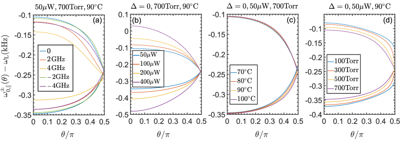
Figure SM1: Precession frequencies $\omega_{0,\parallel}^{\pm}$ with respect to the Larmor frequency $\omega_{\mathrm{L}}$ under different conditions. The external magnetic field $B_{0}=55\mu$T.

SM2.2 Nuclear Zeeman effect on the precession frequency

The driving Hamiltonian $H_{D}\propto S_{x}\cos\theta-S_{z}\sin\theta$. Since $\rho_{0}$ has only diagonal terms, in $\left[S_{z},\rho_{0}\right]$ only terms $\left|F_{1}m\right\rangle_{SS}\left\langle F_{2}m\right|$ with $F_{1}\neq F_{2}$ exists which has large energy $\Delta_{S}$ in the superspace. Thus, we can neglect the term $S_{z}\sin\theta$ in $H_{D}$. We can further apply the rotating-wave approximation and ignore the term $S_{z}\sin\theta$ in $S_{\parallel}\left(\omega\right)$ since the mixing rate of $\left|Fm\right\rangle_{SS}\left\langle Fm\right|$ and $\left|F^{\prime}m\right\rangle_{SS}\left\langle F^{\prime}m\pm 1\right|$ is much smaller that the Larmor frequency $\omega_{\mathrm{L}}$.

Figure SM2: Difference of the precession frequencies with and without the NuZ effect: $\omega_{0,\parallel/\perp}^{+}\left(\text{with NuZ}\right)-\omega_{0,\parallel/\perp}^{+}\left(\text{without NuZ}\right)$. Here, the solid lines are for the case with parallel probe lasers, while the dotted-dash lines are for the vertical ones.

Under our experimental conditions, $S_{\parallel/\perp}^{\pm}\left(\omega\right)=0$ has two solutions around $\pm\omega_{\mathrm{L}}$, respectively, where in the superscript, “$+/-$” represents the $\sigma^{+}/\sigma^{-}$ polarization. Here, we focus on the solution $\omega_{0}$ around $+\omega_{\mathrm{L}}$. From Eq. (SM24) we have

$$S_{\parallel}^{\pm}\left(\omega\right)=-2\mathrm{Re}\left[\mathrm{Tr}\left(S_{x}\left(\mathcal{L}_{0}^{eff}\mp i\omega\right)^{-1}\mathcal{L}_{1}\rho_{0}\right)\right]\cos\theta$$ (SM25)

and

$$S_{\perp}^{\pm}\left(\omega\right)=\mp 2\mathrm{Im}\left[\mathrm{Tr}\left(S_{y}\left(\mathcal{L}_{0}^{eff}\mp i\omega\right)^{-1}\mathcal{L}_{1}\rho_{0}\right)\right]\cos\theta.$$ (SM26)

The precession frequency for the parallel probe laser case is plotted in Fig. SM1 for different (a) detunings $\Delta$, (b) pump powers, (c) temperatures, and (d) densities of nitrogen gas. The external field $B_{0}=55\mu$T.

To show quantitatively the NuZ effect on the precession frequency, we plot the deviation of the precession frequencies with and without considering the NuZ effect in Fig. SM2 under different conditions as in Fig. SM1. We can see that the NuZ effect lowers the precession frequency by an amount smaller than the linear NuZ splitting $\omega_{\text{NuZ}}$ ($226$Hz) because the $a$-manifold has a frequency $\omega_{\text{L}}-\omega_{\text{NuZ}}$ while the $b$-manifold has a frequency $\omega_{\text{L}}+\omega_{\text{NuZ}}$. As $\theta$ changes, the deviation $\omega_{0,\parallel}^{+}\left(\text{with NuZ}\right)-\omega_{0,\parallel}^{+}\left(\text{without NuZ}\right)$ becomes more negative while $\omega_{0,\perp}^{+}\left(\text{with NuZ}\right)-\omega_{0,\perp}^{+}\left(\text{without NuZ}\right)$ gets less negative because of the opposite contribution from the $b$ manifold (See Sec. ). Here, we only show the deviation for $\omega_{0,\parallel/\perp}^{+}$ because the contribution from the NuZ effect to the precession frequency is the same for $\omega_{0,\parallel/\perp}^{+}$ and $\omega_{0,\parallel/\perp}^{-}$. The proof is as follows. As shown in Eq. (SM25), for $\sigma^{+}$ pump laser, $\omega_{0,\parallel}^{+}$ is determined by

$$S_{\parallel}^{+}\left(\omega_{0,\parallel}^{+}\right)=-2\mathrm{Re}\left[\mathrm{Tr}\left(S_{x}\left(\mathcal{L}_{0}^{eff}\left(B_{0}\right)-i\omega_{0,\parallel}^{+}\right)^{-1}\mathcal{L}_{1}\rho_{0}\right)\right]\cos\theta=0.$$ (SM27)

For $\sigma^{-}$ pump laser, which is equivalent to inverting the magnetic field $B_{0}$ while keeping the pump laser’s helicity the same, $\omega_{0,\parallel}^{-}$ is determined by

$$S_{\parallel}^{-}\left(\omega_{0,\parallel}^{-}\right)=-2\mathrm{Re}\left[\mathrm{Tr}\left(S_{x}\left(\mathcal{L}_{0}^{eff}\left(-B_{0}\right)+i\omega_{0,\parallel}^{-}\right)^{-1}\mathcal{L}_{1}\rho_{0}\right)\right]\cos\theta=0.$$ (SM28)

When the NLZ effect and LS are neglected and only the NuZ effect is considered,

$$S_{\parallel}^{-}\left(\omega_{0,\parallel}^{-}\right) = -2\mathrm{Re}\left[\mathrm{Tr}\left(S_{x}\left(\mathcal{L}_{0}^{eff}\left(-B_{0}\right)+i\omega_{0,\parallel}^{-}\right)^{-1}\mathcal{L}_{1}\rho_{0}\right)^{\ast}\right]\cos\theta$$ (SM29)

$$= 2\mathrm{Re}\left[\mathrm{Tr}\left(S_{x}\left(\mathcal{L}_{0}^{eff}\left(B_{0}\right)-i\omega_{0,\parallel}^{-}\right)^{-1}\mathcal{L}_{1}\rho_{0}\right)\right]\cos\theta$$

$$= -S_{\parallel}^{+}\left(\omega_{0,\parallel}^{-}\right).$$

The case for $\omega_{0,\perp}^{+}$ and $\omega_{0,\perp}^{-}$ can be proved similarly from Eq. (SM26). Therefore, $\omega_{0,\parallel/\perp}^{+}=\omega_{0,\parallel/\perp}^{-}$ when considering only the NuZ effect.

SM2.3 Asymmetric heading errors

Under the rotating-wave approximation, in $\mathcal{L}_{1}\rho_{0}$ in Eqs. (SM25) and (SM26), only terms $\left|a,m\right\rangle_{SS}\left\langle a,m+1\right|$ and $\left|b,m+1\right\rangle_{SS}\left\langle b,m\right|$ need to be taken into account. In this basis, the $B_{0}$-dependent diagonal terms of $\mathcal{L}_{0}^{eff}$ are in the diagonal terms as(ignoring the small modification of the hyperfine states resulting from the interaction to the external field $\vec{B}_{0}$)

$$E\left(a,m+1\right)-E\left(a,m\right)\approx\omega_{\mathrm{L}}-\omega_{\mathrm{NuZ}}-\left(2m+1\right)\omega_{\mathrm{rev}},$$ (SM30)

$$E\left(b,m\right)-E\left(b,m+1\right)\approx\omega_{\mathrm{L}}+\omega_{\mathrm{NuZ}}-\left(2m+1\right)\omega_{\mathrm{rev}}.$$ (SM31)

As a result, $S_{\parallel/\perp}^{+}\left(\omega\right)$ is a function of $\alpha_{m}^{a,b}\left[\omega_{\mathrm{L}}-\sigma^{a,b}\omega_{\mathrm{NuZ}}-\left(2m+1\right)\omega_{\mathrm{rev}}-\omega\right]$, where $\alpha_{m}^{a,b}$ is a coefficient dependent on the manifold $a$, $b$, and the magnetic number $m$, but independent of $\omega$ and $B_{0}$, $\sigma^{a}=1$ and $\sigma^{b}=-1$. For $\sigma^{-}$ polarization, or equivalently for negative $B_{0}$, similarly, in $\mathcal{L}_{1}\rho_{0}$, only terms $\left|a,m\right\rangle_{SS}\left\langle a,m+1\right|$ and $\left|b,m+1\right\rangle_{SS}\left\langle b,m\right|$ need to be considered and $S_{\parallel/\perp}^{-}\left(\omega\right)$ is the same/opposite function of $\alpha_{m}^{a,b}\left[-\omega_{\mathrm{L}}+\sigma^{a,b}\omega_{\mathrm{NuZ}}-\left(2m+1\right)\omega_{\mathrm{rev}}+\omega\right]$. Therefore, the solutions $\omega_{0,\shortparallel/\perp}^{\pm}$ to the equations $S_{\parallel/\perp}^{+}\left(\omega_{0,\shortparallel/\perp}^{+}\right)=0$ and $S_{\parallel/\perp}^{-}\left(\omega_{0,\shortparallel/\perp}^{-}\right)=0$ fulfill

$$\omega_{0,\parallel/\perp}^{+}+\omega_{0,\parallel/\perp}^{-}=2\omega_{\mathrm{L}}$$ (SM32)

if the NuZ splitting $\omega_{\mathrm{NuZ}}$ is ignored, i.e., the heading errors for $\sigma^{+}$ and $\sigma^{-}$ polarizations are symmetric:

$$\omega_{0,\parallel/\perp}^{+}\left(\theta_{1}\right)-\omega_{0,\parallel/\perp}^{+}\left(\theta_{2}\right)=\omega_{0,\parallel/\perp}^{-}\left(\theta_{2}\right)-\omega_{0,\parallel/\perp}^{-}\left(\theta_{1}\right).$$ (SM33)

However, the existence of $\omega_{\mathrm{NuZ}}$ does not only shifts $\left(\omega_{0,\parallel/\perp}^{+}+\omega_{0,\parallel/\perp}^{-}\right)/2-\omega_{\mathrm{L}}$ from zero, but breaks the symmetry (SM33), as shown in Figs. (2) and (3). As shown in the last subsection, the NuZ effect contributes the same to the precession frequencies $\omega_{0,\parallel/\perp}^{+}$ and $\omega_{0,\parallel/\perp}^{-}$, which is $\theta$-dependent, so the heading errors including all three sources are not symmetric for $\sigma^{+}$ and $\sigma^{-}$ polarizations.

The precession frequencies $\omega_{0,\parallel}$ for the parallel probe laser case and the corresponding heading errors are shown in Fig. SM3 for different external fields $B_{0}$ and pumping powers, while other parameters are the same as in Fig. 2(a). When the power of the pump laser is lower or the external magnetic field is smaller, the heading errors for both $\sigma^{+}$ and $\sigma^{-}$ polarizations are smaller. The former is because the population changes in the Zeeman states with smaller Rabi frequencies become smaller as the tilted angle $\theta$ varies, while the latter is because the NLZ and NuZ induced frequency deviations become smaller. In all these cases, the heading errors for $\sigma^{+}$ and $\sigma^{-}$ polarizations are asymmetric: with $\sigma^{+}$-polarized pumps, the heading error is smaller. Same as Fig. 2, here we only compare the theoretical results with the experimental data on the heading errors, because the real magnetic fields slightly deviate from $30$, $50$, $70\mu\mathrm{T}$. These differences can not be determined accurately in our experiment, but they are small so that the NLZ effect and the NuZ effect induced by them can be ignored. Therefore, the heading errors $\omega_{0}\left(\theta\right)-\omega_{0}\left(0\right)$ are the same as in the $B_{0}=30$, $50$, $70\mu\mathrm{T}$ cases. The relatively large deviation between the theoretical and experimental results Figs. SM2(b) and (f) is resulting from the remnant magnetization in the magnetic shield, which has a more obvious effect for smaller field $B_{0}$.

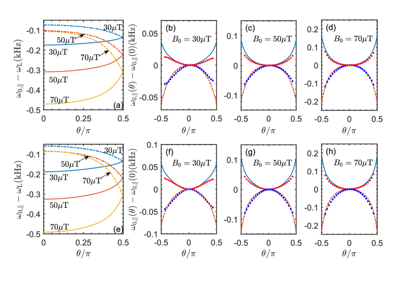
Figure SM3: (a) Precession frequencies $\omega_{0,\parallel}^{\pm}$ with respect to the Larmor frequency $\omega_{\mathrm{L}}$ and heading errors $\omega_{0}\left(\theta\right)-\omega_{0}\left(0\right)$ (b)-(d) for different $B_{0}$ with the probe laser parallel to the RF field. Experimental data are plotted in red dots ($\sigma^{+}$ polarization) and blue diamonds ($\sigma^{-}$ polarization). The power of the pump laser is $50\mu$W, and its detuning $\Delta=0$. (e)-(h) Same as (a)-(d), but with a larger pump power of $90\mu$W.

The heading errors in a broad parameter regime for $B_{0}=55\mu\mathrm{T}$ are plotted in Fig. SM4, which also shows asymmetry for the $\sigma^{+}$ and $\sigma^{-}$ polarizations. To give a physical insight of the heading error under different conditions, we show the average value $\left\langle F_{z}\right\rangle$ in the insets, where $F_{z}=S_{z}+I_{z}$ is the total spin’s angular moment along the $z$ direction. The mean value $\left\langle F_{z}\right\rangle$ reveals the connection between the heading errors and the atomic populations in the Zeeman levels: the heading error increases monotonously as $\left\langle F_{z}\right\rangle$ changes faster as the tilted angle $\theta$ varies. For instance, as shown in Fig. SM4(c), as the temperature increases, the change of the polarization $\left\langle F_{z}\right\rangle$ becomes smaller since the hotter cell has less nitrogen gas. As a result, the heading error gets smaller.

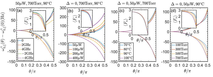
Figure SM4: Heading errors $\omega_{0,\parallel}^{\pm}\left(\theta\right)-\omega_{0,\parallel}^{\pm}\left(0\right)$ under various conditions. The inset shows the mean value of the total spin’s angular moment in the $z$ direction $\left\langle F_{z}\right\rangle$ for the $\sigma^{+}$-polarized pump. For the $\sigma^{-}$ case, $\left\langle F_{z}\right\rangle$ is the opposite.

SM3 Reduction of heading errors using two pump lasers with opposite helicities

In geophysical surveys to detect magnetic anomalies of various types such as searching for mineral deposits or locating lost objects, the relative angle between the object and the magnetometer is not well-known and it varies with time, leading to accuracy degradation for high-accuracy magnetometers. For instance, with the parameters shown in Fig. 4(a), to achieve the accuracy of $1$pT around $\theta=60^{\circ}$, one needs to acquire the angle with an uncertainty of $\left(1.56\times 10^{-3}\right)^{\circ}$ (blue solid curve), which is almost impossible to reach. Hence, the heading error results in accuracy degradation and needs to be reduced.

In this section, we study the compensation of the heading errors by summing up the measured precession frequencies from atomic vapor cells pumped by lasers with opposite helicities.

SM3.1 Both probe lasers parallel or perpendicular to the AC driving fields

When the probe lasers are parallel or perpendicular to the AC driving fields in both cells, it has been proved in the last section (see Eq. (SM33)) that the heading errors induced by the NLZ effect and LS can be canceled by averaging the output from magnetometers pumped by opposite-helicity lasers. However, the NuZ effect breaks the symmetry of the heading errors in these two atomic cells, giving the monotonously increasing heading errors as the tilted angle $\theta$ increases, as shown in Figs. 2(a) and 2(b).

Since the asymmetry of the heading errors comes from the opposite contributions of the NuZ splitting $\omega_{\text{NuZ}}$ to the $a$ and $b$ manifolds, increasing the populations or reducing the change of the populations in the $a$-manifold can reduce the heading error in the averaged precession frequencies from the two cells. In Fig. SM5, the heading errors $\left[\omega_{0,\parallel/\perp}^{+}\left(\theta\right)+\omega_{0,\parallel/\perp}^{-}\left(\theta\right)-\omega_{0,\parallel/\perp}^{+}\left(0\right)-\omega_{0,\parallel/\perp}^{-}\left(0\right)\right]/2$ are shown for $B_{0}=55\mu$T while other parameters such as the laser’ detuning $\Delta$ and power, the temperature, and the density of the nitrogen gas are varied. The populations in the $a$ manifold $P_{a}=$Tr$\rho_{0}^{\left(a\right)}$ are shown in the corresponding insets. We see from Fig. SM5(a) that the heading error is smaller when the detuning $\Delta$ is around $0$ where the transition between the $b$-manifold and the excited states is resonant with the pump laser and the population in the $b$ manifold is suppressed. In Fig. SM5(b), the heading errors do not change much as the power of the pump laser varies, since lowering the input power decreases not only the population and but its change in the $a$-manifold. However, the case in (c) and (d) is different: when lowing the temperature or the density of the buffer gas, the population in the $a$ manifold increases while its change decreases, and thus the heading error is reduced. Note that this uncompensated heading error in Fig. SM5 results from the NuZ effect, so it does not only show the deviation of the heading errors when the NuZ is not considered, but gives the improvement one can acquire by choosing the $\sigma^{+}$-polarized ($\sigma^{-}$-polarized) pump laser other than the $\sigma^{-}$-polarized ($\sigma^{+}$-polarized) one with the parallel (vertical) probe laser.

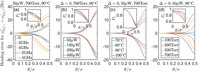
Figure SM5: Heading errors in the average of two magnetometers pumped by opposite-helicity lasers and probe by lasers in the same directions. The external field $B_{0}=55\mu$T. The insets show the atomic populations in the $a$-manifold.

SM3.2 One probe laser parallel and another perpendicular to the AC driving fields

Tuning the parameters of the two cells with the probe lasers both parallel or perpendicular to the driving fields can weaken the NuZ-effect on the heading errors but can not compensate for it. For this, we propose to employ one probe laser parallel and another perpendicular to the driving fields in this two-cell scheme. This can be understood simply as the following: we approximate $S_{\parallel/\perp}\left(\omega\right)\approx-g_{e}\mu_{\mathrm{B}}B_{1}\left[S^{a}\left(\omega\right)\pm S^{b}\left(\omega\right)\right]\cos\theta$ with the plus sign for $S_{\parallel}\left(\omega\right)$ and minus sign for $S_{\perp}\left(\omega\right)$, where

$$S^{a}\left(\omega\right)=\mathrm{Re}\left[\mathrm{Tr}\left(S_{+}\left(\mathcal{L}_{0}^{eff}-i\omega\right)^{-1}\mathcal{L}_{1-}\rho_{0}^{\left(a\right)}\right)\right],$$ (SM34)

$$S^{b}\left(\omega\right)=\mathrm{Re}\left[\mathrm{Tr}\left(S_{-}\left(\mathcal{L}_{0}^{eff}-i\omega\right)^{-1}\mathcal{L}_{1+}\rho_{0}^{\left(b\right)}\right)\right],$$ (SM35)

for $\sigma^{+}$ polarization, while

$$S^{a}\left(\omega\right)=\mathrm{Re}\left[\mathrm{Tr}\left(S_{+}\left(\mathcal{L}_{0}^{eff}+i\omega\right)^{-1}\mathcal{L}_{1-}\rho_{0}^{\left(a\right)}\right)\right],$$ (SM36)

$$S^{b}\left(\omega\right)=\mathrm{Re}\left[\mathrm{Tr}\left(S_{-}\left(\mathcal{L}_{0}^{eff}+i\omega\right)^{-1}\mathcal{L}_{1+}\rho_{0}^{\left(b\right)}\right)\right],$$ (SM37)

for $\sigma^{-}$ polarization (in the treatment here, we invert $\vec{B}_{0}$ instead of the healicity of the pump). Here, $\mathcal{L}_{1\pm}\rho=-i\left[S_{\pm},\rho\right]$ and $\rho_{0}^{\left(a/b\right)}$ is the density matrix projected in the $a/b$-manifold: $\rho_{0}^{\left(F=a,b\right)}=\sum_{mm^{\prime}}\left|Fm\right\rangle_{SS}\left\langle Fm\right|\rho_{0}\left|Fm^{\prime}\right\rangle_{SS}\left\langle Fm^{\prime}\right|$. Consequently, in the parallel case, the precession frequency $\omega_{0,\parallel}^{\pm}$ for parallel probe lasers is determined by $S^{a}\left(\omega_{0,\parallel}^{\pm}\right)+S^{b}\left(\omega_{0,\parallel}^{\pm}\right)=0$ while the precession frequency $\omega_{0,\perp}^{\pm}$ for the perpendicular case is determined by $S^{a}\left(\omega_{0,\perp}^{\pm}\right)-S^{b}\left(\omega_{0,\perp}^{\pm}\right)=0$. Since the contribution from the $a$-manifold is lager, we expand $S^{a/b}\left(\omega\right)$ around $\omega_{a}^{\pm}$ as

$$S^{a}\left(\omega\right)\approx C_{a}^{\pm}\left(\omega-\omega_{a}^{\pm}\right)$$ (SM38)

and

$$S^{b}\left(\omega\right)\approx C_{b}^{\pm}\left(\omega-\omega_{a}^{\pm}\right)+D^{\pm},$$ (SM39)

where $C_{a}^{\pm}$, $C_{a}^{\pm}$, and $D^{\pm}$ are constants with the plus sign in the superscript for $B_{0}>0$ and minus sign for $B_{0}<0$. When the NLZ effect and the LS are neglected, similar to Eq. (LABEL:sm8) we have

$$\omega_{a}^{+}=\omega_{a}^{-}=\omega_{\mathrm{L}}-\omega_{\mathrm{NuZ}},$$

$C_{a}^{+}=-C_{a}^{-}$, and $D_{a}^{+}=-D_{a}^{-}$. Therefore, the solutions are

$$\omega_{0,\parallel}^{\pm}=\omega_{\mathrm{L}}-\omega_{\mathrm{NuZ}}-\frac{D^{\pm}}{C_{a}^{\pm}+C_{b}^{\pm}}$$ (SM40)

and

$$\omega_{0,\perp}^{\pm}=\omega_{\mathrm{L}}-\omega_{\mathrm{NuZ}}+\frac{D^{\pm}}{C_{a}^{\pm}-C_{b}^{\pm}}.$$ (SM41)

In the limit $\left|C_{a}^{\pm}\right|\gg\left|C_{b}^{\pm}\right|$, which is the case in our parameter regime, the NuZ-induced heading errors in $\omega_{0,\parallel}^{\pm}+\omega_{0,\perp}^{\mp}$ are canceled.

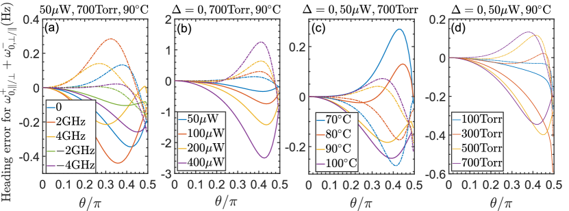
Figure SM6: Same as Fig. SM4, but for averaging cells probed by lasers in different directions (one parallel to the RF driving field while another perpendicular to it). Here, solid lines are for $\omega_{0,\parallel}^{+}+\omega_{0,\perp}^{-}$ and dotted-dash lines are for $\omega_{0,\perp}^{+}\left(\theta\right)+\omega_{0,\parallel}^{-}\left(\theta\right)$.

With the same parameters as in Fig. SM5, we plot the heading errors $\left[\omega_{0,\parallel/\perp}^{+}\left(\theta\right)+\omega_{0,\perp/\parallel}^{-}\left(\theta\right)-\omega_{0,\parallel/\perp}^{+}\left(0\right)-\omega_{0,\perp/\parallel}^{-}\left(0\right)\right]/2$ in Fig. SM6. Because of the large cancellation of the NuZ effect, the heading errors are well suppressed in a wide parameter regime.

SM4 Heading errors compensated by an auxiliary field

We have shown in Fig. 4 that the measured precession frequency has a smaller angular dependence by using an auxiliary field. For instance, with an auxiliary field of $15$nT (purple solid curve in Fig. 4(a)), to achieve the accuracy of $1$pT around $\theta=60^{\circ}$, the required uncertainty in the angle $\theta$ becomes $\left(2.67\times 10^{-2}\right)^{\circ}$. In the application, the strength and sometimes the direction of the magnetic field in the circumstance where the magnetometer works are roughly known. Therefore, we can calibrate the magnetometer in the lab with an auxiliary field, considering a 2% difference of the magnetic field strength. Within this difference, we have shown our auxiliary-field method is robust.

In this section, we give an insight into our heading-error-compensation method by employing a small auxiliary magnetic field, and compare it with some other methods in the literature. At the large relaxation regime, the atomic system’s density matrix can be approximated by the spin-temperature distribution Appelt et al. (1998)

$$\rho=\exp\left(\beta F_{z}\right)/\text{Tr}\left[\exp\left(\beta F_{z}\right)\right],$$ (SM42)

where the parameter $\beta$ is connected to the electron’s polarization as

$$\exp\left(\beta\right)=\left(1+2\left\langle S_{z}\right\rangle\right)/\left(1-2\left\langle S_{z}\right\rangle\right).$$ (SM43)

Applying the linear response theory and summing up incoherently the transition frequencies between two adjacent states using the weight in $\left[S_{x},\rho\right]$, one can acquire the precession frequency $\omega_{0}$. Note from Eq. (4), the polarization $\left\langle S_{z}\right\rangle$ for $\sigma^{+}$-polarized pump can be approximated as

$$\left\langle S_{z}\right\rangle = \frac{R_{op}\left[\left(\cos\theta+1\right)^{2}-\left(\cos\theta-1\right)^{2}\right]}{2R_{op}\left[\left(\cos\theta+1\right)^{2}+\left(\cos\theta-1\right)^{2}\right]+2\Gamma_{rel}}$$ (SM44)

$$= \frac{2R_{op}\cos\theta}{R_{op}\left[\left(\cos\theta+1\right)^{2}+\left(\cos\theta-1\right)^{2}\right]+2\Gamma_{rel}}.$$

where $R_{op}$ is the optical pumping rate for a $\sigma^{+}$-polarized pump laser that can be obtained by adiabatically eliminating the excited states, and $\Gamma_{rel}$ is the relaxation rate. Therefore, for small $\theta$, one can expand $\cos\theta$ around $1$ and obtain the angular dependence of $\omega_{0}$ as $-\cos\theta$ for $\sigma^{+}$-polarized pump laser and $\cos\theta$ for the $\sigma^{-}$-polarized pump laser (note that the polarization $\left\langle S_{z}\right\rangle$ is inverted for $\sigma^{-}$-polarized pump). With the small auxiliary field, the total precession frequency is shown in Eq. (7) where the cosine function can cancel the angular dependence in $\omega_{0}\left(\theta,B_{a}=0\right)$ by properly choosing $B_{a}$. This is why the compensation is excellent in Fig.4(b) for small $\theta$. For large $\theta$, the compensation is getting worse since higher orders terms of $\cos\theta$ become more important. However, mathematically, one can always find an amplitude $B_{a}$ to make the derivative $\partial_{\theta}\omega_{0}\left(\theta,B_{a}\right)=\partial_{\theta}\omega_{0}\left(\theta,B_{a}=0\right)-\mathrm{sign}\left(\sigma^{\pm}\right)\mu_{\mathrm{eff}}B_{\mathrm{a}}\sin\theta$ vanish at some angle $\theta_{0}$. Then the heading error is flattened within some angular interval around $\theta_{0}$, as shown in Fig. 4(c).

Our method is a compensation way to reduce the heading error. Following the analysis above, we can obtain a lengthy expression of the precession frequency. But we have theoretically simplified the model by, for instance, ignoring the incoherent coupling between each adjacent transitions, which may result in deviations from the exact result, and in the setup, there might be remnant magnetic field parallel or antiparallel to the sensor’s direction that can also be compensated by the auxiliary field, so the best way in practical use is to measure the heading error under controllable conditions first, then determine the auxiliary field according to the measured data.

In the literature, apart from the compensation methods using two magnetometers pumped by opposite-helicity lasers Yabuzaki and Ogawa (1974); Scholtes et al. (2012); Oelsner et al. (2019), some other methods are proposed to reduce the heading error. For example, the cancelation of NLZ effect with LS Jensen et al. (2009); Chalupczak et al. (2010), the spin-locking method using a RF field Bao et al. (2018), and the synchronous optical pumping with double-modulation of the lasers Seltzer et al. (2007). However, they have all concentrated on the NLZ effect and the LS, but neglected the NuZ effect. Thus when the atomic population in the $b$ manifold (or the $a$ manifold if the pump laser is resonant with it) increases, which is usually the case when the sensor is more tilted (note that it is not the case in the pulsed-pump magnetometer where the populations in each manifold remain the same), those methods are less effective Lee et al. (2021). In contrast, our method by using the auxiliary field can still flatten the heading error at large $\theta$ by tuning the auxiliary field $B_{a}$, which helps increase the accuracy of magnetometers working around a certain angle.

References

Kominis et al. (2003)
I. K. Kominis,
T. W. Kornack,
J. C. Allred,
and M. V.
Romalis, Nature (London)
422, 596 (2003),
ISSN 0028-0836.
Hovde et al. (2011)
C. Hovde,
B. Patton,
O. Versolato,
E. Corsini,
S. Rochester,
and D. Budker,
in Defense + Commercial Sensing
(2011).
Colombo et al. (2017)
S. Colombo,
V. Dolgovskiy,
T. Scholtes,
Z. D. Grujić,
V. Lebedev,
and A. Weis,
Applied Physics B: Lasers and Optics
123, 35 (2017).
Scholtes et al. (2012)
T. Scholtes,
V. Schultze,
R. IJsselsteijn,
S. Woetzel, and
H.-G. Meyer,
Optics express 20,
29217 (2012),
URL https://doi.org/10.1364/OE.20.029217.
(25)
See Supplemental Material at [] for demonstration of the system
symmetry and the NuZ effect on the heading errors in different parameter
regimes, comparison between two proposals using cells with opposite-helicity
pumps, and elaboration of our auxiliary-field method and its comparison with
other methods in the literature, which also contains Refs.
[11,14,17-20,22-24,26-30,33].
Happer et al. (2010)
W. Happer,
Y.-Y. Jau, and
T. Walker,
Optically Pumped Atoms (Wiley,
New York, 2010).
Walls and Milburn (2008)
D. F. Walls and
G. J. Milburn,
Quantum Optics, SpringerLink: Springer e-Books
(Springer Berlin, 2008), ISBN
9783540285731,
URL https://books.google.com.sg/books?id=LiWsc3Nlf0kC.
Gardiner and Zoller (2004)
C. Gardiner and
P. Zoller,
Quantum Noise: A Handbook of Markovian and
Non-Markovian Quantum Stochastic Methods with Applications to Quantum
Optics, Springer Series in Synergetics
(Springer,Berlin, Heidelberg, 2004),
ISBN 9783540223016,
URL https://books.google.com.sg/books?id=a_xsT8oGhdgC.
Fetter and Walecka (2012)
A. L. Fetter and
J. D. Walecka,
Quantum Theory of Many-Particle Systems
(Dover, Mineola, New York, 2012).
(31)
In this equality, we have neglected the corrections in the
Hyperfined states from the external magnetic field. When including it,
without the NuZ effet, the average value slightly deviates from the Larmor
frequency, as shown in the inset in Fig. 3(a).
(32)
In our experiment, instead of changing the helicity of the pump
laser, we invert the external field, which can be proved to be equivalent.
Compared with the good agreement between the theoretical and experimental
results in the left-handed-circular-polarization case, the relatively larger
deviation in the right-handed case is probably because of the change of
system parameters in the experiment when the external field is inverted.