A new discrete distribution arising from a generalised
random game and its asymptotic properties
R. Frühwirth^∗1, R. Malina² and W. Mitaroff ^1
1Institute of High Energy Physics, Austrian Academy of Sciences, Vienna, Austria
²CH-8330 Pfäffikon (ZH), Switzerland

 

Abstract
The rules of a game of dice are extended to a “hyper-die” with $n\in\mathbb{N}$ equally probable faces, numbered from 1 to $n$. We derive recursive and explicit expressions for the probability mass function and the cumulative distribution function of the gain $G_{n}$ for arbitrary values of $n$. A numerical study suggests the conjecture that for $n\to\infty$ the expectation of the scaled gain $\mathbb{E}\,[H_{n}]=\mathbb{E}\,[G_{n}/\sqrt{n}\,]$ converges to $\sqrt{\pi/\,2}$. The conjecture is proved by deriving an analytic expression of the expected gain $\mathbb{E}\,[G_{n}]$. An analytic expression of the variance of the gain $G_{n}$ is derived by a similar technique. Finally, it is proved that $H_{n}$ converges weakly to the Rayleigh distribution with scale parameter 1.
Keywords: Random game; Mlynar distribution; Expected gain; Asymptotic behaviour; Weak
convergence; Rayleigh distribution
2010 Mathematics Subject Classification: 00A08; 60E05

1 Introduction

The German popular science journal “Bild der Wissenschaft” features a monthly column, “Heinrich Hemme’s Cogito”, posing a mathematical or logical puzzle. The November 2015 column presented the rules of a game of dice, called “Mlynář” (“Miller” in Czech) [1], allegedly popular in Bohemia, but actually invented by the author [2]. The puzzle asked for calculating a player’s average or expected gain.

The game is played with a standard die having faces numbered 1 to 6. Each player throws the die up to five times and collects a gain or a penalty $G_{6}$ according to the following rules:

• If $1^{\mathrm{st}}$ throw shows a [1], the gain is $G_{6}=1$ point, and the player stops. Else:

• If $2^{\mathrm{nd}}$ throw shows [1] or [2], the gain is $G_{6}=2$ points, the player stops. Else:

• If $3^{\mathrm{rd}}$ throw shows [1] to [3], the gain is $G_{6}=3$ points, the player stops. Else:

• If $4^{\mathrm{th}}$ throw shows [1] to [4], the gain is $G_{6}=4$ points, the player stops. Else:

• If $5^{\mathrm{th}}$ throw shows [1] to [5], the gain is $G_{6}=5$ points, the player stops. Else:

• Without a further throw, the gain is $G_{6}=6$ points, and the player stops.

Assuming a fair die, the probability of each face showing up is ${1}/{6}$. Hence, the probabilities $p_{k,6}=\mathbb{P}\,(G_{6}=k)$ of a player gaining $k$ points can be easily computed, see Eqs. (2.2)–(2.4). The expected value of the gain, i.e., the average number of points a player will collect in the long run, is defined by

$$\mathbb{E}\,[G_{6}]=\sum_{k=1}^{6}\,k\cdot p_{k,6}=2.7747\>\mathrm{points,}$$ (1.1)

where the $p_{k,6}$ are calculated by one of Eqs. (2.2)–(2.4) for $n=6$. They are plotted in Fig. 1(a).

2 Generalisation

An interesting one-parametric discrete distribution arises if the game is generalised by replacing the ordinary die with a “hyper-die” having $n\in\mathbb{N}$ equally probable faces and formalising the rules in the following way.

Let $\bm{X}=\{X_{k},\ k\geq 1\}$ be a stochastic process such that the $X_{k}$ are independent and identically distributed according to the discrete uniform distribution on the set $\{1,2,\ldots,n\}$. Let $G_{n}$ be the gain associated with $\bm{X}$​, and $\tau$ be a stopping time with respect to $\bm{X}$. Then the game is defined by the following rule:

$$\text{\bf Rule of the game:}\quad\mathrm{For}\ k=1,2,\ldots,n:\quad X_{k}\leq k\ \Longrightarrow\ \tau=k,\ G_{n}=k.$$ (2.1)

It follows that the probability mass function $p_{k,n}=\mathbb{P}\,(G_{n}=k)$ of the gain $G_{n}$ is recursively defined by

$$p_{1,n}=\frac{1}{n}\,,\quad p_{k,n}=\left(1-\sum_{i=1}^{k-1}\,p_{i,n}\right)\cdot\frac{k}{n}=p_{k-1,n}\cdot k\cdot\left(\frac{1}{k-1}-\frac{1}{n}\right)\quad\text{for}\quad 2\leq k\leq n.$$ (2.2)

The last probability is $p_{n,n}=1-\sum_{i=1}^{n-1}p_{i,n}$, and the sum of all probabilities is $\sum_{k=1}^{n}\,p_{k,n}=1$ as required. The probabilities in Eq. (2.2) can also be expressed explicitely by

$$p_{k,n}=\frac{1}{n}\cdot\prod_{i=2}^{k}\,i\cdot\left(\frac{1}{i-1}-\frac{1}{n}\right)\quad\text{for}\quad 2\leq k\leq n,$$ (2.3)

or more conveniently by

$$p_{k,n}=\frac{k}{n^{k}}\cdot\frac{(n-1)\,!}{(n-k)\,!}\quad\text{for}\quad 1\leq k\leq n.$$ (2.4)

While the recursive definition in Eq. (2.2) is well suited to numerical computations (see below and Section 3), the expression in Eq. (2.4) is the most useful one for the further theoretical analysis (see Sections 4 and 5).

To the best of our knowledge, this distribution has not been described in the literature before. We propose to call it the “Mlynar distribution” with parameter $n$. As another example, the probability mass function for the case $n=25$ is plotted in Fig. 1(b).

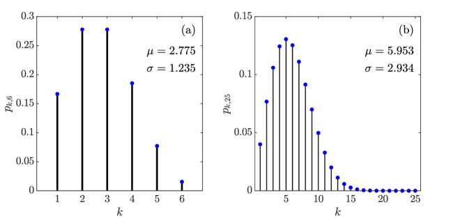
Figure 1: Probabilities $p_{k,n}$ for (a) $n=6$, (b) $n=25$

The cumulative distribution function (cdf) $P_{n}(x)=\mathbb{P}\,(G_{n}\leq x)$ of $G_{n}$ is obtained by summing over the probabilities in Eq. (2.4) up to $\chi=\lfloor x\rfloor$, the largest integer that does not exceed $x$:

$$P_{n}(x)=\sum_{i=1}^{\chi}\,p_{i,n}=1-\frac{(n-1)\,!}{n^{\chi}\,(n-1-\chi)\,!}\quad\text{with}\quad\chi=\lfloor x\rfloor.$$ (2.5)

The mode of the distribution can be determined by rewriting Eq. (2.2) in the following form:

$$p_{k,n}=p_{k-1,n}\cdot\phi_{k,n},\quad\text{with}\quad\phi_{k,n}=\frac{nk-(k-1)\,k}{nk-n}\quad\text{for}\quad 2\leq k\leq n.$$ (2.6)

It is easily verified that $\phi_{k,n}$ is a monotonically decreasing function of $k$ for fixed $n$. Hence, the probability mass function $p_{k,n}$ is unimodal and the mode $m$ is the largest integer $k$ such that $\phi_{k,n}\geq 1$.

If $n$ can be expressed as $n=(m-1)\cdot m$, then $\phi_{m,n}=1$, and both values $m-1$ and $m$ are modes; see for example Fig. 1(a) where $n=6=2\cdot 3$. Otherwise, the mode $m$ is the floor of the positive solution of the quadratic equation $k^{2}-k=n$:

$$m=\left\lfloor\textstyle\frac{1}{2}+\sqrt{\textstyle\frac{1}{4}+n}\right\rfloor.$$ (2.7)

As an example, see Fig. 1(b) where $n=25$ and $m=\lfloor 5.5249\ldots\rfloor=5$.

The expectation of $G_{n}$ is given by

$$g(n)=\mathbb{E}\,[G_{n}]=\sum_{k=1}^{n}\,k\cdot p_{k,n}=(n-1)\,!\cdot\sum_{k=1}^{n}\,\frac{k^{2}}{n^{k}\cdot(n-k)\,!}.$$ (2.8)

Using Eq. (2.2), the function $g(n)$ can be calculated in double precision floating point arithmetic without numerical problems for $n$ up to $10^{15}$. As can be seen in Fig. 1(b), the $p_{k,n}$ fall off very quickly in the tail of the distribution already for $n=25$. If $K(n)$ is the index in the sum in Eq. (2.8) beyond which addition of another term has no effect because of rounding errors, then $K(n)\leq 8.5\sqrt{n}$ for $1\leq n\leq 10^{15}$.

As guessed initially and proved below in Section 4, $g(n)\sim C\sqrt{n}$ as $n\to\infty$, with $C\in\mathbb{R}$. Therefore, a scaled expectation $h(n)$ is defined as

$$h(n)=\mathbb{E}\,[H_{n}]=\frac{g(n)}{\sqrt{n}},\quad\text{with}\quad H_{n}=\frac{G_{n}}{\sqrt{n}}.$$ (2.9)

$H_{n}$ will be called the scaled gain in the following. The functions $g(n)$ and $h(n)$ are plotted in Fig. 2(a) and (b), respectively, in the range $1\leq n\leq 25$.

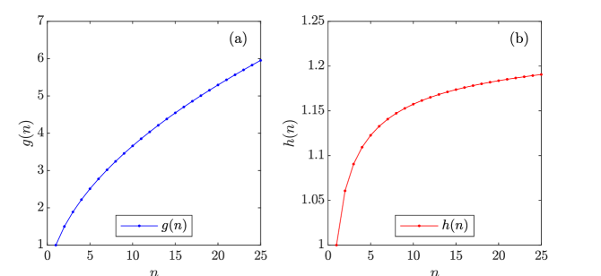
Figure 2: (a) $g(n)$ up to $n=25$. (b) $h(n)$ up to $n=25$.

3 Empirical conjecture

The function $h(n)$ is monotonically increasing and apparently converges to a non-zero constant value, as shown in Fig. 3(a) up to $n=10^{10}$, with a logarithmic scale on the abscissa. A surprising observation reveals this constant to be empirically equal (within our numerical precision) to $\sqrt{\pi/2}$. This inspires us to the following conjecture:

Conjecture 3.1.

The scaled expectation value $h(n)$ converges for $n\to\infty$ as

$$\lim_{n\to\infty}h(n)=\lim_{n\to\infty}\mathbb{E}\,[H_{n}]=\sqrt{\frac{\pi}{2}}=1.2533\dots.$$ (3.1)

In order to corroborate the conjecture, the difference function

$$\Delta(n)=\sqrt{\frac{\pi}{2}}-h(n)$$ (3.2)

is calculated and plotted in Fig. 3(b) up to $n=10^{10}$ with a logarithmic scale on the abscissa.

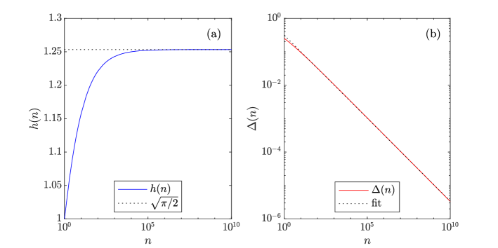
Figure 3: (a) Function $h(n)$. (b) $\Delta(n)$ in Eq. (3.2) and the fitted power function.

Its behaviour above $n=10$ shows approximate linearity in double log scale, suggesting an ansatz $\Delta(n)=c\cdot n^{-s}$ or

$$\log_{10}\Delta(n)=\alpha+\beta\cdot\log_{10}n,\quad\text{with}\quad\alpha=\log_{10}c,\quad\beta=-s.$$ (3.3)

The intercept $\alpha$ and the slope $\beta$ have been estimated by linear regression [4] on 10 data points ($n_{\mathrm{df}}=8$) situated at $\log_{10}n=1,2,\ldots,10$, yielding the estimates

$$\tilde{\alpha}=-0.4996\pm 0.0068,\ \tilde{\beta}=-\tilde{s}=-0.4970\pm 0.0011,\ \tilde{c}=10^{\tilde{\alpha}}=0.3165\pm 0.0050,$$ (3.4)

where the errors represent $1\,\sigma$.

Assuming that above ansatz holds beyond $n=10^{10}$, the extrapolation $n\to\infty$ adds strong evidence for the exact validity of Eq. (3.1). The asymptotic behaviour of $h(n)$ can thus be parametrized, within the fitted accuracy, by

$$h(n)=\frac{1}{\sqrt{n}}\cdot\mathbb{E}\,[G_{n}]\approx\sqrt{\frac{\pi}{2}}-\Delta(n),\quad\text{with}\quad\Delta(n)=0.3165\cdot n^{-0.4970}.$$ (3.5)

It is remarkable that within $2.7\,\sigma$, $\tilde{s}\approx 0.5$, hinting at $\Delta(n)\propto{1}/{\sqrt{n}}$.

4 Proof of the conjecture

In order to prove Conjecture 3.1, we first derive an explicit expression for the expected gain $g(n)=\mathbb{E}\,[G_{n}]$ for fixed $n$.

Proposition 4.1.

For any $n\in\mathbb{N}$, $g(n)=\mathbb{E}\,[G_{n}]$ is given by

$$g(n)=\sum_{k=1}^{n}\,k\cdot p_{k,n}=\mathrm{e}^{n}\,n^{-n}\,\Gamma(n+1,n)-1,$$ (4.1)

where $\Gamma(a,x)$ is the upper incomplete Gamma function as defined in [5] and [6, Eq. (6.5.3)].

Proof.

The sum in Eq. (4.1) can be rewritten in the following way:

$$\sum_{k=1}^{n}\,k\cdot p_{k,n}=\sum_{k=1}^{n}\,\sum_{i=k}^{n}\,p_{i,n}.$$ (4.2)

It is easy to see that in the double sum on the right hand side $p_{1,n}$ occurs exactly once, $p_{2,n}$ occurs exactly twice, and so on, up to $p_{n,n}$ which occurs exactly $n$ times. The same is true for the sum on the left hand side.

The resulting double sum in Eq. (4.2) can be evaluated in two steps, with the help of [5]. In the first step we obtain

$$P_{k,n}=\sum_{i=k}^{n}\,p_{i,n}=\frac{(n-1)\,!}{n^{k-1}\,(n-k)\,!}.$$ (4.3)

The second step yields

$$\mathbb{E}\,[G_{n}]=\sum_{k=1}^{n}\,P_{k,n}=\mathrm{e}^{n}\,n^{-n}\,\Gamma(n+1,n)-1=g(n).$$ (4.4)

This concludes the proof. ∎

The asymptotic behaviour of $h(n)$ as $n\to\infty$ is given by the following proposition.

Proposition 4.2.

Let $h(n)$ be as in Eq. (2.9). Then, as $n\to\infty$,

$$h(n)\sim\sqrt{\frac{\pi}{2}}-\frac{1}{3\sqrt{n}}\quad\Longrightarrow\quad\lim_{n\to\infty}h(n)=\sqrt{\frac{\pi}{2}}.$$ (4.5)

Proof.

The asymptotic behaviour of $\Gamma(n+1,n)$ as $n\to\infty$ is given in [6, Eq. (6.5.35)]:

$$\Gamma(n+1,n)\sim\mathrm{e}^{-n}\,n^{n}\,\left(\sqrt{\frac{n\,\pi}{2}}+\frac{2}{3}+\frac{\sqrt{2\,\pi}}{24\,\sqrt{n}}+\cdots\right).$$ (4.6)

It follows that as $n\to\infty$

$$g(n)\sim-1+\sqrt{\frac{n\,\pi}{2}}+\frac{2}{3}+\frac{\sqrt{2\,\pi}}{24\,\sqrt{n}}+\cdots=\sqrt{\frac{n\,\pi}{2}}-\frac{1}{3}+\frac{\sqrt{2\,\pi}}{24\,\sqrt{n}}+\cdots.$$ (4.7)

Dividing by $\sqrt{n}$ and omitting terms that are $\mathcal{O}(1/n)$ yields Eq. (4.5). ∎

It should be noted that the empirical result in Eq. (3.5) is in very good agreement with the assertion of the proposition.

5 Variance and asymptotic distribution

The variance of $G_{n}$ can be computed as $\mathbb{V}\,[G_{n}]=\mathbb{E}\,[G_{n}^{\,2}]-\mathbb{E}\,[G_{n}]^{2}$. The following proposition gives an explicit expression for $\mathbb{V}\,[G_{n}]$.

Proposition 5.1.

The variance of $G_{n}$ is given by

$$\mathbb{V}\,[G_{n}]=2\,n-\mathbb{E}\,[G_{n}]-\mathbb{E}\,[G_{n}]^{2}.$$ (5.1)

Proof.

The expectation of $G_{n}^{\,2}$ can be rewritten in the following form:

$$\mathbb{E}\,[G_{n}^{\,2}]\,=\,\sum_{k=1}^{n}k^{2}\cdot p_{k,n}=\sum_{k=1}^{n}\sum_{i=1}^{k}\,(2\,i-1)\cdot p_{k,n}=\sum_{k=1}^{n}\,(2\,k-1)\cdot P_{k,n}.$$ (5.2)

It is not difficult to verify that in all sums $p_{1,n}$ occurs exactly once, $p_{2,n}$ occurs exactly four times, and so on, up to $p_{n,n}$ which occurs exactly $n^{2}$ times. With the help of [5] and using Eq. (4.4), the last sum evaluates to

$$\mathbb{E}\,[G_{n}^{\,2}]=2\cdot\sum_{k=1}^{n}\,k\cdot P_{k,n}-\sum_{k=1}^{n}\,P_{k,n}=2\,n-\mathbb{E}\,[G_{n}].$$ (5.3)

Subtracting the squared expectation yields the proposition. ∎

The function $v(n)$ is defined by $v(n)=\mathbb{V}\,[H_{n}]=\mathbb{V}\,[G_{n}/\sqrt{n}\,]=\mathbb{V}\,[G_{n}]/n$. Its asymptotic behaviour as $n\to\infty$ is described by the following proposition.

Proposition 5.2.

As $n\to\infty$,

$$v(n)\sim 2-\frac{\pi}{2}-\sqrt{\frac{\pi}{18\,n}}+\cdots\quad\Longrightarrow\quad\lim_{n\to\infty}v(n)=2-\frac{\pi}{2}.$$ (5.4)

Proof.

The assertion follows by an elementary calculation from Eqs. (4.7) and (5.1). ∎

A well-known distribution with mean $\sqrt{\pi/\,2}$ and variance $2-\pi/\,2$ ist the Rayleigh distribution with scale parameter $\sigma=1$ [7]. Its cdf $R(x)$ is given by

$$R(x)=\begin{cases}1-\exp(-x^{2}/\,2)&\quad\text{for}\quad x\geq 0,\\ 0&\quad\text{for}\quad x<0.\end{cases}$$ (5.5)

The following proposition shows that this distribution is indeed the asymptotic distribution of $H_{n}$ for $n\to\infty$.

Proposition 5.3.

The sequence ($H_{n},\ n\in\mathbb{N}$) converges weakly (in distribution) to a random variable with the cdf $R(x)$ in Eq. (5.5):

$$\lim_{n\to\infty}Q_{n}(x)=1-\exp(-x^{2}/\,2),\quad\text{for}\quad x\geq 0,$$ (5.6)

where $Q_{n}(x)$ is the cdf of $H_{n}$ (see also Eq. (2.5)):

$$Q_{n}(x)=P_{n}(x\sqrt{n})=1-\frac{(n-1)\,!}{n^{\chi}\,(n-1-\chi)\,!}\quad\text{with}\quad\chi=\lfloor x\sqrt{n}\rfloor.$$ (5.7)

Proof.

As $P_{n}(x)$ is increasing, the following inequality holds:

$$P_{n}(x\sqrt{n}-1)\leq P_{n}(\lfloor x\sqrt{n}\rfloor)\leq P_{n}(x\sqrt{n}).$$ (5.8)

We rewrite $P_{n}$ in the form

$$P_{n}(u)=1-\exp(L(u)),\quad\text{with}\quad L(u)=\ln\Gamma(n)-u\ln n-\ln\Gamma(n-u).$$ (5.9)

According to [6, Eq. (6.1.41)], $\ln\Gamma(z)$ can be approximated by

$$\ln\Gamma(z)\sim(z-\textstyle\frac{1}{2})\cdot\ln(z)-z+\textstyle\frac{1}{2}\cdot\ln(2\,\pi),\quad\text{for}\quad z\to\infty.$$ (5.10)

With this approximation, we obtain:

$$L(u)=\ln\left(n\right)\,\left(n-\textstyle\frac{1}{2}\right)-u+\ln\left(n-u\right)\,\left(u-n+\textstyle\frac{1}{2}\right)-u\,\ln\left(n\right).$$ (5.11)

Using [8] and [5] for the calculation of the limits in Eq. (5.12), as well as the fact that $L(u)$ is decreasing, we obtain that

$$\lim_{n\to\infty}L(x\sqrt{n}-1)=\lim_{n\to\infty}L(x\sqrt{n})=-\frac{x^{2}}{2}\ \Longrightarrow\ \lim_{n\to\infty}L(\lfloor x\sqrt{n}\rfloor)=-\frac{x^{2}}{2}.$$ (5.12)

It follows that

$$\lim_{n\to\infty}Q_{n}(x)=\lim_{n\to\infty}P_{n}(\lfloor x\sqrt{n}\rfloor)=1-\exp(-x^{2}/\,2).$$ (5.13)

This concludes the proof. ∎

The convergence in distribution is illustrated by Fig 4. It shows that already for $n=10^{4}$ it is virtually impossible to visually distinguish $Q_{n}(x)$ and $R(x)$. A numerical study shows that the maximum absolute difference $d(n)=\max_{x}|Q_{n}(x)-R(x)|$ can be parametrized by $d_{n}\approx 0.44/\sqrt{n}$ for $n\geq 100$.

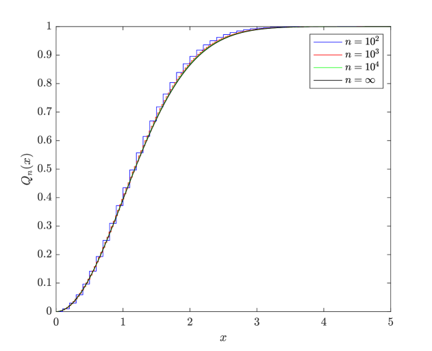
Figure 4: Distribution functions of $H_{n}$ and the limiting Rayleigh cdf.

6 Conclusions

Inspired by an elementary puzzle, we have analyzed the generalisation of a game of dice to a “hyper-die” with an arbitrary number $n$ of faces. The gain of a player is described by a novel probability mass function and its corresponding cumulative distribution function. We propose to call the distribution the “Mlynar distribution” with parameter $n$.

An empirical study has led to the conjecture that the expectation of the scaled gain converges to the constant $\sqrt{\pi/\,2}$. A proof of the conjecture has been found, based on an analytic expression of the gain. A simple expression for the variance of the gain has been derived as well, thereby proving that the variance of the scaled gain converges to $2-\pi/2$.

Finally, it has been proved that the scaled gain converges weakly (in distribution) to the Rayleigh distribution with scale parameter 1.

Authors’ contributions

This work was carried out in collaboration of all authors. Authors RM and WM defined the generalized game, mainly contributed Sects. 2 and 3, and wrote the first draft of the manuscript. Author RF fully contributed Sects. 4 and 5, and completed and finalized the manuscript. All authors have read and approved the submitted manuscript.

Competing interests

The authors declare that no competing interests exist.

——————————————————————————————————————————————— ©2021 R. Frühwirth, R. Malina and W. Mitaroff. This is an Open Access article distributed under the terms of the Creative Commons Attribution License http://creativecommons.org/licenses/by/2.0, which permits unrestricted use, distribution, and reproduction in any medium, provided the original work is properly cited.

References

- [1] Hemme H. Cogito. Bild der Wissenschaft. 2015; 52(11):100. ISSN 0006-2375. German.
- [2] Hemme H. Private communication. Received 26 February 2021.
- [3] Sigman K. Lecture Notes on Stochastic Modeling I, ch. 3. Accessed 15 February 2021. Available: www.columbia.edu/~ks20/stochastic-I/stochastic-I-ST.pdf.
- [4] Lyons L. Statistics for nuclear and particle physicists. Cambridge (UK): Cambridge University Press; 1986.
- [5] Wolfram Research. WolframAlpha — computational intelligence. Accessed 15 February 2021. Available: www.wolframalpha.com.
- [6] Abramowitz M, Stegun I. Handbook of Mathematical Functions. 8th printing. New York: Dover Publications; 1970.
- [7] Johnson NL, Kotz S, Balakrishnan N. Continuous Univariate Distributions. Vol. 1, 2nd ed. New York: John Wiley & Sons; 1994.
- [8] The Mathworks, Inc. MATLAB® Symbolic Toolbox™. Accessed 15 February 2021. Available: www.mathworks.com/help/symbolic.