A Verified Decision Procedure for Univariate Real Arithmetic with the BKR Algorithm

Abstract

We formalize the univariate fragment of Ben-Or, Kozen, and Reif’s (BKR) decision procedure for first-order real arithmetic in Isabelle/HOL. BKR’s algorithm has good potential for parallelism and was designed to be used in practice. Its key insight is a clever recursive procedure that computes the set of all consistent sign assignments for an input set of univariate polynomials while carefully managing intermediate steps to avoid exponential blowup from naively enumerating all possible sign assignments (this insight is fundamental for both the univariate case and the general case). Our proof combines ideas from BKR and a follow-up work by Renegar that are well-suited for formalization. The resulting proof outline allows us to build substantially on Isabelle/HOL’s libraries for algebra, analysis, and matrices. Our main extensions to existing libraries are also detailed.

1 Introduction

Formally verified arithmetic has important applications in formalized mathematics and rigorous engineering domains. For example, real arithmetic questions (first-order formulas in the theory of real closed fields) often arise as part of formal proofs for safety-critical cyber-physical systems (CPS) [29], the formal proof of the Kepler conjecture involves the verification of more than $23,000$ real inequalities [13], and the verification of floating-point algorithms also involves real arithmetic reasoning [14]. Some real arithmetic questions involve $\forall$ and $\exists$ quantifiers; these quantified real arithmetic questions arise in, e.g., CPS proofs, geometric theorem proving, and stability analysis of models of biological systems [35].

Quantifier elimination (QE) is the process by which a quantified formula is transformed into a logically equivalent quantifier-free formula. Tarski famously proved that the theory of first-order real arithmetic (FOL_R) admits QE; FOL_R validity and satisfiability are therefore decidable by QE and evaluation [36]. Thus, in theory, all it takes to rigorously answer any real arithmetic question is to verify a QE procedure for FOL_R. However, in practice, QE algorithms for FOL_R are complicated and the fastest known QE algorithm, cylindrical algebraic decomposition (CAD) [6] is, in the worst case, doubly exponential in the number of variables. The multivariate CAD algorithm is highly complicated and has yet to be fully formally verified in a theorem prover [18], although various specialized approaches have been used to successfully tackle restricted subsets of real arithmetic questions in proof assistants, e.g., quantifier elimination for linear real arithmetic [25], sum-of-squares witnesses [15] or real Nullstellensatz witnesses [30] for the universal fragment, and interval arithmetic when the quantified variables range over bounded domains [16, 33].

There are few general-purpose formally verified decision procedures for FOL_R. Mahboubi and Cohen [5] formally verified an algorithm for QE based on Tarski’s proof but their formalization is primarily a theoretical decidability result [5, Section 1] owing to the non-elementary complexity of Tarski’s algorithm. The proof-producing procedure by McLaughlin and Harrison [22] can solve a number of small multivariate examples but suffers similarly from the complexity of the underlying Cohen-Hörmander procedure. The situation for univariate real arithmetic (i.e., problems that involve only a single variable) is better. In Isabelle/HOL, Li, Passmore, and Paulson [18] formalized an efficient univariate decision procedure based on univariate CAD. There are additionally some univariate decision procedures in PVS, including $\mathtt{hutch}$ [23] (based on CAD) and $\mathtt{tarski}$ [24] (based on the Sturm-Tarski theorem).

This paper adds to the latter body of work by formalizing the univariate case of Ben-Or, Kozen, and Reif’s (BKR) decision procedure [2] in Isabelle/HOL [26, 27]. Our formalization of univariate BKR is ${\approx}7000$ lines [8]. Our main contributions are:

• In Section 2, we present an algorithmic blueprint for implementing BKR’s procedure that blends insights from Renegar’s [32] later variation of BKR. Compared to the original abstract presentations [2, 32], our blueprint is phrased concretely in terms of matrix operations which facilitates its implementation and identifies its correctness properties.

• Our blueprint is designed for formalization by judiciously combining and fleshing out BKR’s and Renegar’s proofs. In Section 3, we outline key aspects of our proof, its use of existing Isabelle/HOL libraries, and our contributions to those libraries.

It is desirable to have a variety of formally verified decision procedures for arithmetic since different strategies can have different efficiency tradeoffs on different classes of problems [7, 30]. For example, in PVS, $\mathtt{hutch}$ is usually significantly faster than $\mathtt{tarski}$ [23] but there are a number of adversarial problems for $\mathtt{hutch}$ on which $\mathtt{tarski}$ performs better [7]. BKR has a fundamentally different working principle than CAD; like the Cohen-Hörmander procedure, it represents roots and sign-invariant regions abstractly, instead of via computationally expensive, real algebraic numbers required in CAD. Further, unlike Cohen-Hörmander, BKR was designed to be used in practice: when its inherent parallelism is exploited, an optimized version of univariate BKR is an NC algorithm (that is, it runs in parallel polylogarithmic time). Our formalization is not yet optimized and parallelized, so we do not yet achieve such efficiency. However, we do export our Isabelle/HOL formalization to Standard ML (SML) and are able to solve some examples with the exported code (Section 3.3).

Additionally, our formalization is a significant stepping stone towards the multivariate case, which builds inductively on the univariate case. We give some (informal) mathematical intuition for multivariate BKR in Appendix A—since multivariate BKR seems to rely fairly directly on the univariate version, we hope that it will be significantly easier to formally verify than multivariate CAD, which is highly complicated. However, it is unlikely that multivariate BKR will be as efficient as CAD in the average case. While BKR states that their multivariate algorithm is computable in parallel exponential time (or in NC for fixed dimension), Canny later found an error in BKR’s analysis of the multivariate case [3], which highlights the subtlety of the algorithm and the role for formal verification. Notwithstanding this, multivariate BKR is almost certain to outperform methods such as Tarski’s algorithm and Cohen-Hörmander and can supplement an eventual formalization of multivariate CAD.

Our formalization is available on the Archive of Formal Proofs (AFP) [8].

2 Mathematical Underpinnings

This section provides an outline of our decision procedure for univariate real arithmetic and its verification in Isabelle/HOL [26]. The goal is to provide an accessible mathematical blueprint that explains our construction and its blend of ideas from BKR [2] and Renegar [32]; in-depth technical discussion of the formal proofs is largely deferred to Section 3. Our procedure starts with two transformation steps (Sections 2.1 and 2.2) that simplify an input decision problem into a so-called restricted sign determination format. An algorithm for the latter problem is then presented in Section 2.3. Throughout this paper, unless explicitly specified, we are working with univariate polynomials, which we assume to have variable $x$. Our decision procedure works for polynomials with rational coefficients (rat poly in Isabelle), though some lemmas are proved more generally for univariate polynomials with real coefficients (real poly in Isabelle).

2.1 From Univariate Problems to Sign Determination

Formulas of univariate real arithmetic are generated by the following grammar, where $p$ is a univariate polynomial with rational coefficients:

$$\phi,\psi~{}\mathrel{::=}~{}p>0~{}|~{}p\geq 0~{}|~{}p=0~{}|~{}\phi\lor\psi~{}|~{}\phi\land\psi$$

In Isabelle/HOL, we define this grammar in fml, which is our type for formulas.

For formula $\phi$, the universal decision problem is to decide if $\phi$ is true for all real values of $x$, i.e., validity of the quantified formula $\forall x{\,}\phi$. The existential decision problem is to decide if $\phi$ is true for some real value of $x$, i.e., validity of the quantified formula $\exists x{\,}\phi$. For example, a decision procedure should return false for formula (1) and true for formula (2) below (left).

$$\forall x{\,}(x^{2}-2=0\land 3x>0)$$ (1)

$$\exists x{\,}(x^{2}-2=0\land 3x>0)$$ (2)

Formula Structure: $$\leavevmode\hbox to13.34pt{\vbox to13.34pt{\text{[drawing]}}}=0\land\leavevmode\hbox to13.04pt{\vbox to13.04pt{\text{[drawing]}}}>0$$

Polynomials: $$\leavevmode\hbox to13.34pt{\vbox to13.34pt{\text{[drawing]}}}:x^{2}-2,\quad\leavevmode\hbox to13.04pt{\vbox to13.04pt{\text{[drawing]}}}:3x$$

The first observation is that both univariate decision problems can be transformed to the problem of finding the set of consistent sign assignments (also known as realizable sign assignments [1, Definition 2.34]) of the set of polynomials appearing in the formula $\phi$.

Definition 1.

A sign assignment for a set $G$ of polynomials is a mapping $\sigma$ that assigns each $g\in G$ to either $+1$, $-1$, or $0$. A sign assignment $\sigma$ for $G$ is consistent if there exists an $x\in\mathbb{R}$ where, for all $g\in G$, the sign of $g(x)$ matches the sign of $\sigma(g)$.

For the polynomials $x^{2}-2$ and $3x$ appearing in formulas (1) and (2), the set of all consistent sign assignments (written as ordered pairs) is:

$$\{(+1,-1),~{}(0,-1),~{}(-1,-1),~{}(-1,0),~{}(-1,+1),~{}(0,+1),~{}(+1,+1)\}$$

Formula (1) is not valid because consistency of sign assignment $(0,-1)$ implies there exists a real value $x\in\mathbb{R}$ such that conjunct $x^{2}-2=0$ is satisfied but not $3x>0$. Conversely, formula (2) is valid because the consistent sign assignment $(0,+1)$ demonstrates the existence of an $x\in\mathbb{R}$ satisfying $x^{2}-2=0$ and $3x>0$. The truth-value of formula $\phi$ at a given sign assignment is computed by evaluating the formula after replacing all of its polynomials by their respective assigned signs. For example, for the sign assignment $(0,-1)$, replacing by $0$ and by $-1$ in the formula structure underlying (1) and (2) shown above (right) yields $0=0\land-1>0$, which evaluates to false. Validity of $\forall x{\,}\phi$ is decided by checking that $\phi$ evaluates to true at each of its consistent sign assignments. Similarly, validity of $\exists x{\,}\phi$ is decided by checking that $\phi$ evaluates to true at at least one consistent sign assignment.

Our top-level formalized algorithms are called decide_universal and decide_existential, both with type rat poly fml $\Rightarrow$ bool. The definition of decide_existential is as follows (the omitted definition of decide_universal is similar):

definition decide_existential :: "rat poly fml $\Rightarrow$ bool"

where "decide_existential fml = (let (fml_struct,polys) = convert fml in

  find (lookup_sem fml_struct) (find_consistent_signs polys) $\not=$ None)"

Here, convert extracts the list of constituent polynomials polys from the input formula fml along with the formula structure fml_struct, find_consistent_signs returns the list of all consistent sign assignments conds for polys, and find checks that predicate lookup_sem fml_struct is true at one of those sign assignments. Given a sign assignment $\sigma$, lookup_sem fml_struct $\sigma$ evaluates the truth value of fml at $\sigma$ by recursively evaluating the truth of its subformulas after replacing polynomials by their sign according to $\sigma$ using the formula structure fml_struct. Thus, decide_existential returns true iff fml evaluates to true for at least one of the consistent sign assignments of its constituent polynomials.

The correctness theorem for decide_universal and decide_existential is shown below, where fml_sem fml x evaluates the truth of formula fml at the real value x.

theorem decision_procedure:

 "($\forall\,$x::real. fml_sem fml x) $\longleftrightarrow$ decide_universal fml"

 "($\exists\,$x::real. fml_sem fml x) $\longleftrightarrow$ decide_existential fml"

This theorem depends crucially on find_consistent_signs correctly finding all consistent sign assignments for polys, i.e., solving the sign determination problem.

2.2 From Sign Determination to Restricted Sign Determination

The next step restricts the sign determination problem to the following more concrete format: Find all consistent sign assignments $\sigma$ for a set of polynomials $q_{1},\dots,q_{n}$ at the roots of a nonzero polynomial $p$, i.e., the signs of $q_{1}(x),\dots,q_{n}(x)$ that occur at the (finitely many) real values $x\in\mathbb{R}$ with $p(x)=0$. The key insight of BKR is that this restricted problem can be solved efficiently (in parallel) using purely algebraic tools (Section 2.3). Following BKR’s procedure, we also normalize the $q_{i}$’s to be coprime with (i.e. share no common factors with) $p$, which simplifies the subsequent construction for the key step and its formal proof.

Remark 1.

The normalization of $q_{i}$’s to be coprime with $p$ can be avoided using a slightly more intricate construction due to Renegar [32]. We have also formalized this construction but omit full details in this paper as the formalization was completed after acceptance for publication. Its overall structure is quite similar to Section 2.3, and it is available in the AFP alongside our formalization of BKR [8].

Consider as input a set of polynomials (with rational coefficients) $G=\{g_{1},\dots,g_{k}\}$ for which we need to find all consistent sign assignments. The transformation proceeds as follows:

1. Factorize the input polynomials $G$ into a set of pairwise coprime factors (with rational coefficients) $Q=\{q_{1},\dots,q_{n}\}$. This also removes redundant/duplicate polynomials.

   Each input polynomial $g\in G$ can be expressed in the form $g=c\prod_{i=1}^{n}q_{i}^{d_{i}}$ for some rational coefficient $c$ and natural number exponents $d_{i}\geq 1$ so the sign of $g$ is directly recovered from the signs of the factors $q\in Q$. For example, if $g_{1}=q_{1}q_{2}$ and in a consistent sign assignment $q_{1}$ is positive while $q_{2}$ is negative, then $g_{1}$ is negative according to that assignment, and so on. Accordingly, to determine the set of all consistent sign assignments for $G$ it suffices to determine the same for $Q$.

2. Because the $q_{i}$’s are pairwise coprime, there is no consistent sign assignment where two or more $q_{i}$’s are set to zero. So, in any given sign assignment, there is either exactly one $q_{i}$ set to zero, or the $q_{i}$’s are all assigned to nonzero (i.e., +1, -1) signs.

   Now, for each $1\leq i\leq n$, solve the restricted sign determination problem for all consistent sign assignments of $\{q_{1},\dots,q_{n}\}\setminus\{q_{i}\}$ at the roots of $q_{i}$. This yields all consistent sign assignments of $Q$ where exactly one $q_{i}$ is assigned to zero.

3. This step and the next step focus on finding all consistent sign assignments where all $q_{i}$’s are nonzero. Compute a polynomial $p$ that satisfies the following properties:

   1. $p$ is pairwise coprime with all of the $q_{i}$’s,

   2. $p$ has a root in every interval between any two roots of the $q_{i}$’s,

   3. $p$ has a root that is greater than all of the roots of the $q_{i}$’s, and

   4. $p$ has a root that is smaller than all of the roots of the $q_{i}$’s.

   An explicit choice of $p$ satisfying these properties when $q_{i}\in Q$ are squarefree and pairwise coprime is shown in Section 3.1.2. The relationship between the roots of $p$ and the roots of $q_{i}\in Q$ is visualized in Fig. 1. Intuitively, the roots of $p$ (red points) provide representative sample points between the roots of the $q_{i}$’s (black squares).

   

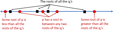
   Figure 1: The relation between the roots of the added polynomial $p$ and the roots of the $q_{i}$’s.

4. Solve the restricted sign determination problem for all consistent sign assignments of $\{q_{1},\dots,q_{n}\}$ at the roots of $p$.

   Returning to Fig. 1, the $q_{i}$’s are sign-invariant in the intervals between any two roots of the $q_{i}$’s (black squares) and to the left and right beyond all roots of the $q_{i}$’s. Intuitively, this is true because moving along the blue real number line in Fig. 1, no $q_{i}$ can change sign without first passing through a black square. Thus, all consistent sign assignments of $q_{i}$ that only have nonzero signs must occur in one of these intervals and therefore, by sign-invariance, also at one of the roots of $p$ (red points).

5. The combined set of sign assignments where some $q_{i}$ is zero, as found in (2), and where no $q_{i}$ is zero, as found in (4), solves the sign determination problem for $Q$, and therefore also for $G$, as argued in (1).

Our algorithm to solve the restricted sign determination problem using BKR’s key insight is called find_consistent_signs_at_roots; we now turn to the details of this method.

2.3 Restricted Sign Determination

The restricted sign determination problem for polynomials $q_{1},\dots,q_{n}$ at the roots of a polynomial $p\neq 0$, where each $q_{1},\dots,q_{n}$ is coprime with $p$, can be tackled naively by setting up and solving a matrix equation. The idea of using a matrix equation for sign determination dates back to Tarski [36] [1, Section 10.3], and accordingly our formalization shares some similarity to Cohen and Mahboubi’s formalization [5] of Tarski’s algorithm (see [4, Section 11.2]). BKR’s additional insight is to avoid the prohibitive complexity of enumerating exponentially many possible sign assignments for $q_{1},\dots,q_{n}$ by computing the matrix equation recursively and performing a reduction that retains only the consistent sign assignments at each recursive step. This reduction keeps intermediate data sizes manageable because the number of consistent sign assignments is bounded by the number of roots of $p$ throughout. We first explain the technical underpinnings of the matrix equation before returning to our implementation of BKR’s recursive procedure. For brevity, references to sign assignments for $q_{1},\dots,q_{n}$ in this section are always at the roots of $p$.

2.3.1 Matrix Equation

The inputs to the matrix equation are a set of candidate (i.e., not necessarily consistent) sign assignments $\tilde{\Sigma}=\{\tilde{\sigma}_{1},\dots,\tilde{\sigma}_{m}\}$ for the polynomials $q_{1},\dots,q_{n}$ and a set of subsets $S=\{I_{1},\dots,I_{l}\}$, $I_{i}\subseteq\{1,\dots,n\}$ of indices selecting among those polynomials. The set of all consistent sign assignments $\Sigma$ for $q_{1},\dots,q_{n}$ is assumed to be a subset of $\tilde{\Sigma}$, i.e., $\Sigma\subseteq\tilde{\Sigma}$.

For example, consider $p=x^{3}-x$ and $q_{1}=3x^{3}+2$. The set of all possible candidate sign assignments $\tilde{\Sigma}=\{(+1),(-1)\}$ must contain the consistent sign assignments for $q_{1}$ (sign $(0)$ is impossible as $p,q_{1}$ are coprime). The possible subsets of indices are $I_{1}=\{\}$ and $I_{2}=\{1\}$.

The main algebraic tool underlying the matrix equation is the Tarski query which provides semantic information about the number of roots of $p$ with respect to another polynomial $q$.

Definition 2.

Given univariate polynomials $p,q$ with $p\neq 0$, the Tarski query $N(p,q)$ is:

$$N(p,q)= \ \#\{x\in\mathbb{R}~{}|~{}p(x)=0,q(x)>0\}-\#\{x\in\mathbb{R}~{}|~{}p(x)=0,q(x)<0\}.$$

Importantly, the Tarski query $N(p,q)$ can be computed from input polynomials $p,q$ using Euclidean remainder sequences without explicitly finding the roots of $p$. This is a consequence of the Sturm-Tarski theorem which has been formalized in Isabelle/HOL by Li [17]. The theoretical complexity for computing $N(p,q)$ is $O(\deg p~{}(\deg p+\deg q))$ [1, Sections 2.2.2 and 8.3]. However, this complexity analysis does not take into account the growth in bitsizes of coefficients in the remainder sequences [1, Section 8.3], so it will not be not achieved by the current Isabelle/HOL formalization of Tarski queries [17] without further optimization.

For the matrix equation, we lift Tarski queries to a subset of the input polynomials:

Definition 3.

Given a univariate polynomial $p\neq 0$, univariate polynomials $q_{1},\dots,q_{n}$, and a subset $I\subseteq\{1,\dots,n\}$, the Tarski query $N(I)$ with respect to $p$ is:

$$N(I)=N(p,\Pi_{i\in I}q_{i})= \ \#\{x\in\mathbb{R}~{}|~{}p(x)=0,\Pi_{i\in I}q_{i}(x)>0\}$$

$$-\#\{x\in\mathbb{R}~{}|~{}p(x)=0,\Pi_{i\in I}q_{i}(x)<0\}.$$

The matrix equation is the relationship $M\cdot w=v$ between the following three entities:

• $M$, the $l$-by-$m$ matrix with entries $M_{i,j}=\Pi_{k\in I_{i}}\tilde{\sigma}_{j}(q_{k})\in\{-1,1\}$ for $I_{i}\in S$ and $\tilde{\sigma}_{j}\in\tilde{\Sigma}$,

• $w$, the length $m$ vector whose entries count the number of roots of $p$ where $q_{1},\dots,q_{n}$ has sign assignment $\tilde{\sigma}$, i.e., $w_{i}=\#\{x\in\mathbb{R}~{}|~{}p(x)=0,\text{sgn}(q_{j}(x))=\tilde{\sigma}_{i}(q_{j})~{}\text{for all}~{}1\leq j\leq n\}$,

• $v$, the length $l$ vector consisting of Tarski queries for the subsets, i.e., $v_{i}=N(I_{i})$.

Observe that the vector $w$ is such that the sign assignment $\tilde{\sigma}_{i}$ is consistent (at a root of $p$) iff its corresponding entry $w_{i}$ is nonzero. Thus, the matrix equation can be used to solve the sign determination problem by solving for $w$. In particular, the matrix $M$ and the vector $v$ are both computable from the input (candidate) sign assignments and subsets. Further, since the subsets will be chosen such that the constructed matrix $M$ is invertible, the matrix equation uniquely determines $w$ and the nonzero entries of $w=M^{-1}\cdot v$.

The following Isabelle/HOL theorem summarizes sufficient conditions on the list of sign assignments signs and the list of index subsets subsets for the matrix equation to hold for polynomial list qs at the roots of polynomial p. Note the switch from set-based representation to list-based representation in the theorem. This formally provides an ordering to the polynomials, sign assignments, and subsets, which is useful for computations.

theorem matrix_equation:

assumes "p$\not=$0"

assumes "$\bigwedge$q. q $\in$ set qs $\Longrightarrow$ coprime p q"

assumes "distinct signs"

assumes "consistent_signs_at_roots p qs $\subseteq$ set signs"

assumes "$\bigwedge$l i. l $\in$ set subsets $\Longrightarrow$ i $\in$ set l $\Longrightarrow$ i < length qs"

shows "M_mat signs subsets *_v w_vec p qs signs = v_vec p qs subsets"

Here, M_mat, w_vec, and v_vec construct the matrix $M$ and vectors $w$, $v$ respectively; *_v denotes the matrix-vector product in Isabelle/HOL. The switch into list notation necessitates some consistency assumptions, e.g., that the signs list contains distinct sign assignments and that the index i occurring in each list of indices l in subsets points to a valid element of the list qs. The proof of matrix_equation uses a counting argument: intuitively, $M_{i,j}$ is the contribution of any real value $x$ that has the sign assignment $\tilde{\sigma}_{j}$ towards $N(I_{i})$, so multiplying these contributions by the actual counts of those real values in $w$ gives $M_{i}\cdot w=v_{i}$.

Note that the theorem does not ensure that the constructed matrix $M$ is invertible (or even square). This must be ensured separately when solving the matrix equation for $w$. We now discuss BKR’s inductive construction and its usage of the matrix equation.

2.3.2 Base Case

The simplest (base) case of the algorithm is when there is a single polynomial $[q_{1}]$. Here, it suffices to set up a matrix equation $M\cdot w=v$ from which we can compute all consistent sign assignments. As hinted at earlier, this can be done with the list of index subsets $[\{\},\{1\}]$ and the candidate sign assignment list $[(+1),(-1)]$. Further, as illustrated in Fig. 2, the matrix $M$ is invertible for these choices of subsets and candidate sign assignments, so the matrix equation can be explicitly solved for $w$.

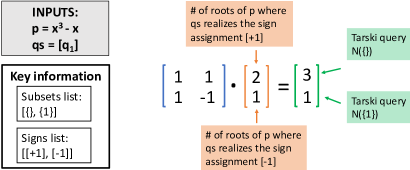
Figure 2: Matrix equation for $p=x^{3}-x$, $q_{1}=3x^{3}+2$.

2.3.3 Inductive Case: Combination Step

The matrix equation can be similarly used to determine the consistent sign assignments for an arbitrary list of polynomials $[q_{1},\dots,q_{n}]$. The driving idea for BKR is that, given two solutions of the sign determination problem at the roots of $p$ for two input lists of polynomials, say, $\ell_{1}=[r_{1},\dots,r_{k}]$ and $\ell_{2}=[r_{k+1},\dots,r_{k+l}]$, one can combine them to yield a solution for the list of polynomials $[r_{1},\dots,r_{k+l}]$. This yields a recursive method for solving the sign determination problem by solving the base case at the single polynomials $[q_{1}],[q_{2}],\dots,[q_{n}]$, and then recursively combining those solutions, i.e., solving $[q_{1},q_{2}],[q_{3},q_{4}],\dots$, then $[q_{1},q_{2},q_{3},q_{4}],\dots$, and so on until a solution for $[q_{1},\dots,q_{n}]$ is obtained. Importantly, BKR performs a reduction (Section 2.3.4) after each combination step to bound the size of the intermediate data.

More precisely, assume for $\ell_{1}$, we have a list of index subsets $S_{1}$ and a list of sign assignments $\tilde{\Sigma}_{1}$ such that $\tilde{\Sigma}_{1}$ contains all of the consistent sign assignments for $\ell_{1}$ and the matrix $M_{1}$ constructed from $S_{1}$ and $\tilde{\Sigma}_{1}$ is invertible. Accordingly, for $\ell_{2}$, we have the list of subsets $S_{2}$, list of sign assignments $\tilde{\Sigma}_{2}$ containing all consistent sign assignments for $\ell_{2}$, and $M_{2}$ constructed from $S_{2}$, $\tilde{\Sigma}_{2}$ is invertible. In essence, we are assuming that $S_{1},\tilde{\Sigma}_{1}$ and $S_{2},\tilde{\Sigma}_{2}$ satisfy the hypotheses for the matrix equation to hold, so that they contain all the information needed to solve for the consistent sign assignments of $\ell_{1}$ and $\ell_{2}$ respectively.

Observe that any consistent sign assignment for $\ell=[r_{1},\dots,r_{k+l}]$ must have a prefix that is itself a consistent sign assignment to $\ell_{1}$ and a suffix that is itself a consistent sign assignment to $\ell_{2}$. Thus, the combined list of sign assignments $\tilde{\Sigma}$ obtained by concatenating every entry of $\tilde{\Sigma}_{1}$ with every entry of $\tilde{\Sigma}_{2}$ necessarily contains all consistent sign assignments for $\ell$. The combined subsets list $S$ is obtained in an analogous way from $S_{1}$, $S_{2}$ (where concatenation is now set union), with a slight modification: the subset list $S_{2}$ indexes polynomials from $\ell_{2}$, but those polynomials now have different indices in $\ell$, so everything in $S_{2}$ is shifted by the length of $\ell_{1}$ before combination. Once we have the combined subsets list, we can calculate the RHS vector $v$ with Tarski queries as explained in Section 2.3.1.

The matrix $M$ constructed from $S$, $\tilde{\Sigma}$ is exactly the Kronecker product of $M_{1}$ and $M_{2}$. Further, the Kronecker product of invertible matrices is invertible, so the matrix equation can be solved for the LHS vector $w$ using $M$ and the vector $v$ computed from the subsets list $S$. Then the nonzero entries of $w$ correspond to the consistent sign assignments of $\ell$. Taking a concrete example, suppose we want to find the list of consistent sign assignments for $\ell=[3x^{3}+2,2x^{2}-1]$ at the zeros of $p=x^{3}-x$. The combination step for $\ell_{1}=[3x^{3}+2]$ and $\ell_{2}=[2x^{2}-1]$ is visualized in Fig. 3.

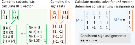
Figure 3: Combining two systems.

2.3.4 Reduction Step

The reduction step takes an input list of index subsets $S$ and candidate sign assignments $\tilde{\Sigma}$. It removes the inconsistent sign assignments and then unnecessary index subsets, which keeps the size of the intermediate data tracked for the matrix equation as small as possible.

The reduction step is best explained in terms of the matrix equation $M\cdot w=v$ constructed from the inputs $S$, $\tilde{\Sigma}$. After solving for $w$, the reduction starts by deleting all indexes of $w_{i}$ that are $0$ and the corresponding $i$-th sign assignments in $\tilde{\Sigma}$ which are now known to be inconsistent (recall that $w_{i}$ counts the number of zeros of $p$ where the $i$-th sign assignment is realized). This corresponds to deleting the $i$-th columns of matrix $M$. If any columns are deleted, the resulting matrix is no longer square (nor invertible). Thus, the next step finds a basis among the remaining rows of the matrix to make it invertible again (deleting any rows that do not belong to the chosen basis). Deleting the $j$-th row in this matrix corresponds to deleting the $j$-th index subset in $S$.

The reduction step for the matrix equation with $p=x^{3}-x$ and $\ell=[3x^{3}+2,2x^{2}-1]$ is visualized in Fig. 4. Naively using the matrix equation for restricted sign determination would require $2^{|\ell|}=4$ Tarski queries for this example, whereas $2+2+4=8$ queries are required using BKR ($2$ for each base case, $4$ for the combination step). However, for longer lists $\ell$, the naive approach requires $2^{|\ell|}$ queries while BKR’s reduction step ensures that the number of intermediate consistent sign assignments is bounded by the number of roots of $p$ (and hence $\deg p$) throughout. This difference is shown in Section 3.3 and is also illustrated by Fig. 4, where $p$ has degree $3$ and there are $3$ consistent sign assignments for $\ell$ after reduction.

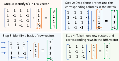
Figure 4: Reducing a system.

3 Formalization

Now that we have set up the theory behind the BKR algorithm, we turn to some details of our formalization: the proofs, extensions to the existing matrix libraries, and the exported code. Our proof builds significantly on existing proof developments in the Archive of Formal Proofs [17, 37, 38]. Isabelle/HOL’s builtin search tool and Sledgehammer [28] provided invaluable automation for discovering existing theorems and for finishing (easy) subgoals in proofs. The most challenging part of the formalization, in our opinion, is the reduction step, in no small part because it involves significant linear algebra (further details in Section 3.2.2).

3.1 Formalizing the Decision Procedure

In this section, we discuss the proofs for our decision procedure in reverse order compared to Section 2; that is, we first discuss the formalization of our algorithm for restricted sign determination find_consistent_signs_at_roots before discussing the top-level decision procedures for univariate real arithmetic, decide_{universal|existential}. The reader may wish to revisit Section 2 for informal intuition behind the procedure while reading this section.

3.1.1 Sign Determination at Roots

We combine BKR’s base case (Section 2.3.2), combination step (Section 2.3.3), and reduction step (Section 2.3.4) to form our core algorithm calc_data for the restricted sign determination problem at the roots of a polynomial. The calc_data algorithm takes a real polynomial p and a list of polynomials qs and produces a $3$-tuple (M, S, $\Sigma$), consisting of the matrix M from the matrix equation, the list of index subsets S, and the list of all consistent sign assignments $\Sigma$ for qs at the roots of p. Although M can be calculated directly from S and $\Sigma$, it is returned (as part of the algorithm), to avoid redundantly recomputing it at every recursive call.

fun calc_data :: "real poly $\Rightarrow$ real poly list $\Rightarrow$ 

  (rat mat $\times$ (nat list list $\times$ rat list list))"

where "calc_data p qs = (let len = length qs in

if len = 0 then

  ($\lambda$(a,b,c).(a,b,map (drop 1) c)) (reduce_system p ([1],base_case_info))

else if len $\leq$ 1 then reduce_system p (qs,base_case_info)

else (let qs1 = take (len div 2) qs; left = calc_data p qs1;

          qs2 = drop (len div 2) qs; right = calc_data p qs2 in

        reduce_system p (combine_systems p (qs1,left) (qs2,right))))"

definition find_consistent_signs_at_roots ::

 "real poly $\Rightarrow$ real poly list $\Rightarrow$ rat list list"

 where "find_consistent_signs_at_roots p qs = 

  (let (M,S,$\Sigma$) = calc_data p qs in $\Sigma$)"

The base case where qs has length $\leq 1$ is handled using the fixed choice of matrix, index subsets, and sign assignments (defined as the constant base_case_info) from Section 2.3.2. Otherwise, when length qs $>1$, the list is partitioned into two sublists qs1, qs2 and the algorithm recurses on those sublists. The outputs for both sublists are combined using combine_systems which takes the Kronecker product of the output matrices and concatenates the index subsets and sign assignments as explained in Section 2.3.3. Finally, reduce_system performs the reduction according to Section 2.3.4, removing inconsistent sign assignments and redundant subsets of indices. The top-level procedure is find_consistent_signs_at_roots, which returns only $\Sigma$ (the third component of calc_data). The following Isabelle/HOL snippets show its main correctness theorem and important relevant definitions.

definition roots :: "real poly $\Rightarrow$ real set" where 

  "roots p = {x. poly p x = 0}"

definition consistent_signs_at_roots :: "real poly $\Rightarrow$ real poly list $\Rightarrow$ 

  rat list set"

where "consistent_signs_at_roots p qs = (sgn_vec qs) ‘ (roots p)"

theorem find_consistent_signs_at_roots:

assumes "p $\not=$ 0"

assumes "$\bigwedge$q. q $\in$ set qs $\Longrightarrow$ coprime p q"

shows "set (find_consistent_signs_at_roots p qs) = 

  consistent_signs_at_roots p qs"

Here, roots defines the set of roots of a polynomial p (non-constructively), i.e., real values x where the polynomial evaluates to 0 (poly p x = 0). Similarly, consistent_signs_at_roots returns the set of all sign vectors for the list of polynomials qs at the roots of p; sgn_vec returns the sign vector for input qs at a real value and ‘ is Isabelle/HOL notation for the image of a function on a set. These definitions are not meant to be computational. Rather, they are used to state the correctness theorem that the algorithm find_consistent_signs_at_roots (and hence calc_data) computes exactly all consistent sign assignments for p and qs for input polynomial p $\not=$ 0 and polynomial list qs, where every entry in qs is coprime to p.

The proof of find_consistent_signs_at_roots is by induction on calc_data. Specifically, we prove that the following properties (our inductive invariant) are satisfied by the base case and maintained by both the combination step and the reduction step:

1. The signs list is well-defined, i.e., the length of every entry in the signs list is the same as the length of the corresponding qs. Additionally, all assumptions on S and $\Sigma$ from the matrix_equation theorem from Section 2.3.1 hold. (In particular, the algorithm always maintains a distinct list of sign assignments that, when viewed as a set, is a superset of all consistent sign assignments for qs.)

2. The matrix M matches the matrix calculated from S and $\Sigma$. (Since we do not directly compute the matrix from S and $\Sigma$, as defined in Section 2.3.1, we need to verify that our computations keep track of M correctly.)

3. The matrix M is invertible (so $M\cdot w=v$ can be uniquely solved for $w$).

Some of these properties are easier to verify than others. The well-definedness properties, for example, are quite straightforward. In contrast, matrix invertibility is more complicated to verify, especially after the reduction step; we will discuss this in more detail in Section 3.2. The inductive invariant establishes that we have a superset of the consistent sign assignments throughout the construction. This is because the base case and the combination step may include extraneous sign assignments. Only the reduction step is guaranteed to produce exactly the set of consistent sign assignments. Thus the other main ingredient in our formalization, besides the inductive invariant, is a proof that the reduction step deletes all inconsistent sign assignments. As calc_data always calls the reduction step before returning output, calc_data returns exactly the set of all consistent sign assignments, as desired.

3.1.2 Building the Univariate Decision Procedure

To prove the decision_procedure theorem from Section 2.1, we need to establish correctness of find_consistent_signs. The most interesting part is formalizing the transformation described in Section 2.2. We discuss the steps from Section 2.2 enumerated (1)–(5) below.

1. Our procedure takes an input list of rational polynomials $G=[g_{1},\dots,g_{k}]$ and computes a list of their pairwise coprime and squarefree factors $Q=[q_{1},\dots,q_{n}]$. An efficient method to factor a single rational polynomial is formalized in Isabelle/HOL by Divasón et al. [11]; we slightly modified their proof to find factors for a list of polynomials while ensuring that the resulting factors are pairwise coprime, which implies that their product $\prod_{i}q_{i}$ is squarefree.

2. This step makes $n$ calls to find_consistent_signs_at_roots, one for each $Q\setminus\{q_{i}\}$.

3. We choose the polynomial $p=(x-\emph{\small crb}(\prod_{i}q_{i}))(x+\emph{\small crb}(\prod_{i}q_{i}))(\prod_{i}q_{i})^{\prime}$, where $(\prod_{i}q_{i})^{\prime}$ is the formal polynomial derivative of $\prod_{i}q_{i}$ and $\emph{\small crb}(\prod_{i}q_{i})$ is a computable positive integer with larger magnitude than any real root of $\prod_{i}q_{i}$. The choice of $\emph{\small crb}(\prod_{i}q_{i})$ uses a proof of the Cauchy root bound [1, Section 10.1] by Thiemann and Yamada [38]. We prove that $p$ satisfies the four properties of step (3) from Section 2.2:

   1. Since $\prod_{i}q_{i}$ is squarefree, $(\prod_{i}q_{i})^{\prime}$ is coprime with $\prod_{i}q_{i}$ and, thus, also coprime with each of the $q_{i}$’s. Because $\emph{\small crb}(\prod_{i}q_{i})$ is strictly larger in magnitude than all of the roots of the roots of the $q_{i}$’s, it follows that $p$ is also coprime with all of the $q_{i}$’s.

   2. By Rolle’s theorem (which is already formalized in Isabelle/HOL’s standard library), $(\prod_{i}q_{i})^{\prime}$ has a root between every two roots of $\prod_{i}q_{i}$ and therefore p also has a root in every interval between any two roots of the $q_{i}$’s.

   3. and iv) This choice of $p$ has roots at $-\emph{\small crb}(\prod_{i}q_{i})$ and $\emph{\small crb}(\prod_{i}q_{i})$, which are respectively smaller and greater than all roots of the $q_{i}$’s.

4. Each polynomial $q_{i}$ is sign invariant between its roots. Accordingly, the $q_{i}$’s are sign invariant between the roots of $\prod_{i}q_{i}$ (and to the left/right of all roots of the $q_{i}$’s).

5. We use the find_consistent_signs_at_roots algorithm with $Q$ and our chosen $p$.

Putting the pieces together, we verify that find_consistent_signs finds exactly the consistent sign assignments for its input polynomials. The decision_procedure theorem follows by induction over the fml type representing formulas of univariate real arithmetic and our formalized semantics for those formulas.

3.2 Matrix Library

Matrices feature prominently in our algorithm: the combination step uses the Kronecker product, while the reduction step requires matrix inversion and an algorithm for finding a basis from the rows (or, equivalently, columns) of a matrix. There are a number of linear algebra libraries available in Isabelle/HOL [9, 34, 37], each building on a different underlying representation of matrices. We use the formalization by Thiemann and Yamada [37] as it provides most of the matrix algorithms required by our decision procedure and supports efficient code extraction [37, Section 1]. Naturally, any such choice leads to tradeoffs; we now detail some challenges of working with the library and some new results we prove.

3.2.1 Combination Step: Kronecker Product

We define the Kronecker product for matrices A, B over a ring as follows:

definition kronecker_product :: "’a :: ring mat $\Rightarrow$ ’a mat $\Rightarrow$ ’a mat"

where "kronecker_product A B = (

let ra = dim_row A; ca = dim_col A; rb = dim_row B; cb = dim_col B in

  mat (ra * rb) (ca * cb)

    ($\lambda$(i,j). A $$ (i div rb, j div cb) * B $$ (i mod rb, j mod cb)))"

Matrices with entries of type ’a are constructed with mat m n f, where m, n :: nat are the number of rows and columns of the matrix respectively, and f :: nat $\times$ nat $\Rightarrow$ ’a is such that f i j gives the matrix entry at position i, j. Accordingly, M $$ (i,j) extracts the (i,j)-th entry of matrix M, and dim_row, dim_col return the number of rows and columns of a matrix respectively.

We prove basic properties of our definition of the Kronecker product: it is associative, distributes over addition, and satisfies the mixed-product identity for matrices A, B, C, D with compatible dimensions (for A * C and B * D):

kronecker_product (A * C) (B * D) =

$$\emph{\small(kronecker\char 95\relax product A B) * (kronecker\char 95\relax product C D)}.$$

The mixed-product identity implies that the Kronecker product of invertible matrices is invertible. Briefly, for invertible matrices A, B with respective inverses A^-1, B^-1, the mixed product identity gives:

(kronecker_product A B) * (kronecker_product A^-1 B^-1) =

$$\emph{\small kronecker\char 95\relax product (A * A${}^{-1}$) (B * B${}^{-1}$) = I},$$

where I is the identity matrix. In other words, kronecker_product A B and kronecker_product A^-1 B^-1 are inverses. We use this to prove that the matrix obtained by the combination step is invertible (part of the inductive hypothesis from Section 3.1.1).

Remark 2.

Prathamesh [31] formalized Kronecker products for Isabelle/HOL’s default matrix type. For computational purposes, we provide a new formalization that is compatible with the matrix representation of Thiemann and Yamada [37].

3.2.2 Reduction Step: Gauss–Jordan and Matrix Rank

Our reduction step makes extensive use of the Gauss–Jordan elimination algorithm by Thiemann and Yamada [39]. First, we use matrix inversion based on Gauss–Jordan elimination to invert the matrix $M$ in the matrix equation (Section 2.3.1 and Step 1 in Fig. 4). We also contribute new proofs surrounding their Gauss–Jordan elimination algorithm in order to use it to extract a basis from the rows (equivalently columns) of a matrix (Step 3 in Fig. 4).

Suppose that an input matrix A has more rows than columns, e.g., the matrix in Step 2 of Fig. 4. The following definition of rows_to_keep returns a list of (distinct) row indices of A.

definition rows_to_keep:: "(’a::field) mat $\Rightarrow$ nat list"

  where "rows_to_keep A = map snd (pivot_positions 

  (gauss_jordan_single (A^T)))"

Here, gauss_jordan_single returns the row-reduced echelon form (RREF) of A after Gauss–Jordan elimination and pivot_positions finds the positions, i.e., (row, col) pairs, of the first nonzero entry in each row of the matrix; both are existing definitions from the library by Thiemann and Yamada [39]. Our main new result for rows_to_keep is:

lemma rows_to_keep_rank:

assumes "dim_col A $\leq$ dim_row A"

shows "vec_space.rank (length (rows_to_keep A)) (take_rows A 

  (rows_to_keep A)) = vec_space.rank (dim_row A) A"

Here vec_space.rank n M (defined by Bentkamp [37]) is the finite dimension of the vector space spanned by the columns of M. Thus, the lemma says that keeping only the pivot rows of matrix A (with take_rows A (rows_to_keep A)) preserves the rank of A. At a high level, the proof of rows_to_keep_rank is in three steps:

1. First, we prove a version of rows_to_keep_rank for the pivot columns of a matrix and where A is assumed to be a matrix in RREF. The RREF assumption for A enables direct analysis of the shape of its pivot columns.

2. Next, we lift the result to an arbitrary matrix A, which can always be put into RREF form by gauss_jordan_single.

3. Finally, we formalize the following classical result that column rank is equal to row rank: vec_space.rank (dim_row A) A = vec_space.rank (dim_col A) (A^T). We lift the preceding results for pivot columns to also work for pivot rows by matrix transposition (pivot rows of matrix A are the pivot columns of the transpose matrix A^T).

To complete the proof of the reduction step, recall that the matrix in Step 2 of Fig. 4 is obtained by dropping columns of an invertible matrix. The resulting matrix has full column rank but more rows than columns. We show that when A in rows_to_keep_rank has full column rank (its rank is dim_col A) then length (rows_to_keep A) = dim_col A and so the matrix consisting of pivot rows of A is square, has full rank, and is therefore invertible.

Remark 3.

Divasón and Aransay formalized the equivalence of row and column rank for Isabelle/HOL’s default matrix type [10] while we have formalized the same result for Bentkamp’s definition of matrix rank [37]. Another technical drawback of our choice of libraries is the locale argument n for vec_space. Intuitively (for real matrices) this carves out subsets of $\mathbb{R}^{\emph{\small n}}$ to form the vector space spanned by the columns of M. Whereas one would usually work with n fixed and implicit within an Isabelle/HOL locale, we pass the argument explicitly here because our theorems often need to relate the rank of vector spaces in $\mathbb{R}^{\emph{\small m}}$ and $\mathbb{R}^{\emph{\small n}}$ for $\emph{\small m}\not=\emph{\small n}$. This negates some of the automation benefits of Isabelle/HOL’s locale system.

3.3 Code Export

We export our decision procedure to Standard ML, compile with mlton, and test it on 10 microbenchmarks from [18, Section 8]. While we leave extensive experiments for future work since our implementation is unoptimized, we compare the performance of our procedure using BKR sign determination (Sections 2.3.2–2.3.4) versus an unverified implementation that naively uses the matrix equation (Section 2.3.1). We also ran Li et al.’s univ_rcf decision procedure [18] which can be directly executed as a proof tactic in Isabelle/HOL (code kindly provided by Wenda Li). The benchmarks were ran on an Ubuntu 18.04 laptop with 16GB RAM and 2.70 GHz Intel Core i7-6820HQ CPU. Results are in Table 1.

The most significant bottleneck in our current implementation is the computation of Tarski queries $N(p,q)$ when solving the matrix equation. Recall for our algorithm (Section 2.3.1) the input $q$ to $N(p,q)$ is a product of (subsets of) polynomials appearing in the inputs. Indeed, Table 1 shows that the algorithm performs well when the factors have low degrees, e.g., ex1, ex2, ex4, and ex5. Conversely, it performs poorly on problems with many factors and higher degrees, e.g., ex3, ex6, and ex7. Further, as noted in experiments by Li and Paulson [20], the Sturm-Tarski theorem in Isabelle/HOL currently uses a straightforward method for computing remainder sequences which can also lead to significant (exponential) blowup in the bitsizes of rational coefficients of the involved polynomials. This is especially apparent for ex6 and ex7, which have large polynomial degrees and high coefficient complexity; these time out without completing even a single Tarski query. From Table 1, the BKR approach successfully reduces the number of Tarski queries as the number of input factors grows—the number of queries for BKR is dependent on the polynomial degrees and the number of consistent sign assignments, while the naive approach always requires exactly $(\frac{n}{2}+1)2^{n}$ queries for $n$ factors (which are reported in Table 1 whether completed or not). On the other hand, there is some overhead for smaller problems, e.g., ex1, ex3, that arises from the recursion in BKR.

The univ_rcf tactic relies on an external solver (we used Mathematica 12.1.1) to produce untrusted certificates which are then formally checked (by reflection) in Isabelle/HOL [18]. This procedure is optimized and efficient: except for ex7 where the tactic timed out, most of the time (roughly 3 seconds per example) is actually spent to start an instance of the external solver.

An important future step, e.g., to enable use of our procedure as a tactic in Isabelle/HOL, is to avoid coefficient growth by using pseudo-division [24, Section 3] or more advanced techniques: for example, using subresultants to compute polynomial GCDs (and thereby build the remainder sequences) [12]. Pseudo-division is also important in the multivariate generalization of BKR (discussed in Appendix A), where the polynomial coefficients of concern are themselves (multivariate) polynomials rather than rational numbers. The pseudo-division method has been formalized in Isabelle/HOL [18], but it is not yet available on the AFP.

Formula	#Poly		#Factor		#$\bm{N(p,q)}$ (Naive)	#$\bm{N(p,q)}$ (BKR)	Time (Naive)	Time (BKR)	Time ([18])
ex1	4	(12)	3	(1)	20	31	0.003	0.006	3.020
ex2	5	(6)	7	(1)	576	180	5.780	0.442	3.407
ex3	4	(22)	5	(22)	112	120	1794.843	1865.313	3.580
ex4	5	(3)	5	(2)	112	95	0.461	0.261	3.828
ex5	8	(3)	7	(3)	576	219	28.608	8.333	3.806
ex6	22	(9)	22	(8)	50331648	-	-	-	6.187
ex7	10	(12)	10	(11)	6144	-	-	-	-
ex1 $\land$ 2	9	(12)	9	(1)	2816	298	317.432	3.027	3.033
ex1 $\land$ 2 $\land$ 4	13	(12)	12	(2)	28672	555	-	51.347	3.848
ex1 $\land$ 2 $\land$ 5	16	(12)	14	(3)	131072	826	-	436.575	3.711

Table 1: Comparison of decision procedures using naive and BKR sign determination and Li et al.’s univ_rcf tactic in Isabelle/HOL [18]. All formulas are labeled following [18, Section 8]; formulas with $\land$ indicate conjunctions of the listed examples. Columns: #Poly counts the number of distinct polynomials appearing in the formula (maximum degree among polynomials in parentheses), #Factor counts the number of distinct factors from (1) in Section 2.2 (maximum degree among factors in parentheses), #$\bm{N(p,q)}$ counts the number of Tarski queries made by each approach, and Time reports time taken (seconds, 3 d.p.) for each decision procedure to run to completion. Cells with - indicate a timeout after 1 hour.

4 Related Work

Our work fits into the larger body of formalized univariate decision procedures. Most closely related are Li et al.’s formalization of a CAD-based univariate QE procedure in Isabelle/HOL [18] and the tarski univariate QE strategy formalized in PVS [24]. We discuss each in turn.

The univariate CAD algorithm underlying Li et al.’s approach [18] decomposes $\mathbb{R}$ into a set of sign-invariant regions, so that every polynomial of interest has constant sign within each region. A real algebraic sample point is chosen from every region, so the set of sample points captures all of the relevant information about the signs of the polynomials of interest for the entirety of $\mathbb{R}$. BKR (and Renegar) take a more indirect approach, relying on consistent sign assignments which merely indicate the existence of points with such signs. Consequently, although CAD will be faster in the average case, BKR and CAD have different strengths and weaknesses. For example, CAD works best on full-dimensional decision problems [21], where only rational sample points are needed (this allows faster computation than the computationally expensive real algebraic numbers that general CAD depends on). The Sturm-Tarski theorem is also invoked in Li et al’s procedure to decide the sign of a univariate polynomial at a point (using only rational arithmetic) [18, Section 5]. (This was later extended to bivariate polynomials by Li and Paulson [19].) This is theoretically similar to our procedure to find the consistent sign assignments for $q_{1},\dots,q_{n}$ at the roots of $p$, as both rely on the mathematical properties of Tarski queries; however, for example, we do not require isolating the real roots of $p$ within intervals, whereas such isolation predicates their computations. This difference reflects our different goals: theirs is to encode algebraic numbers in Isabelle/HOL, ours is to perform full sign determination with BKR.

PVS’s $\mathtt{tarski}$ uses Tarski queries and a version of the matrix equation to solve univariate decision problems [24]. Unlike our work, $\mathtt{tarski}$ has already been optimized in significant ways; for example, $\mathtt{tarski}$ computes Tarski queries with pseudo-divisions. However, $\mathtt{tarski}$ does not maintain a reduced matrix equation as our work does. Further, $\mathtt{tarski}$ was designed to solve existential conjunctive formulas, requiring DNF transformations otherwise [7].

In addition, as previously mentioned, our work is somewhat similar in flavor to Cohen and Mahboubi’s (multivariate) formalization of Tarski’s algorithm [5]. In particular, the characterization of the matrix equation and the parts of the construction that do not involve reduction share considerable overlap, as BKR derives the idea of the matrix equation from Tarski [2]. However, the reduction step is only present in BKR and is a distinguishing feature of our work.

5 Conclusion and Future Work

This paper describes how we have verified the correctness of a decision procedure for univariate real arithmetic in Isabelle/HOL. To the best of our knowledge, this is the first formalization of BKR’s key insight [2, 32] for recursively exploiting the matrix equation. Our formalization lays the groundwork for several future directions, including:

1. Optimizing the current formalization and adding parallelism.

2. Proving that the univariate sign determination problem is decidable in NC [2, 32] and other complexity-theoretic results. This (ambitious) project would require developing a complexity framework that is compatible with all of the libraries we use.

3. Verifying a multivariate sign determination algorithm and decision procedure based on BKR. As mentioned previously, multivariate BKR has an error in its complexity analysis; variants of decision procedures for FOL_R based on BKR’s insight that attempt to mitigate this error could eventually be formalized for useful points of comparison. Two of particular interest are that of Renegar [32], who develops a full QE algorithm, and that of Canny [3], in which coefficients can involve some more general terms, like transcendental functions.

Appendix A Comments on Multivariate BKR

The ultimate intent is for the univariate formalization to serve as the basis for an extension to the multivariate case. The main part of the univariate construction that must be adapted for multivariate polynomials is the computation of Tarski queries. In the univariate case, this is accomplished with remainder sequences per the following (standard) result:

Theorem 1.

[Generalized Sturm’s theorem [32, Proposition 8.1]] Given coprime univariate polynomials $p$, $q$ with $p\neq 0$, form the Euclidean remainder sequence $p_{1}=p$, $p_{2}=p^{\prime}q$, and $p_{i}$ is the negated remainder of $p_{i-2}$ divided by $p_{i-1}$ for $i\geq 3$. This terminates at some $p_{k+1}=0$ because the remainder has lower degree than the divisor at every step. Let $a_{i}$ be the leading coefficient of $p_{i}$ for $1\leq i\leq k$. Consider the two sequences $a_{1},\dots,a_{k}$ and $(-1)^{\deg p_{1}}a_{1},\cdots,(-1)^{\deg p_{k}}a_{k}$. If $S^{+}(p,q)$ is the number of sign changes in $a_{1},\dots,a_{k}$ and $S^{-}(p,q)$ is the number of sign changes in $(-1)^{\deg p_{1}}a_{1},\cdots,(-1)^{\deg p_{k}}a_{k}$, then $N(p,q)=S^{-}(p,q)-S^{+}(p,q)$.

Following the idea of BKR, we intend to treat multivariate polynomials in $n$ variables as univariate polynomials (whose coefficients are polynomials in $n-1$ variables) and so compute remainder sequences of polynomials with attention to a single variable. These remainder sequences will be sequences of polynomials in $n-1$ variables rather than integers, but we only need to know the signs of those polynomials (rather than their values). That reduces the problem of sign determination for polynomials in $n$ variables to a sign determination problem for polynomials in $n-1$ variables. In this way we intend to successively reduce multivariate computations to a series of (already formalized) univariate computations.

This intuition can be captured by the following concrete example. Consider $p=x^{2}y+1$ and $q=xy+1$. Suppose we choose to first eliminate $y$. If $x$ is 0, then the analysis for the remaining $p=q=1$ is simple. Otherwise, both $x$ and $x^{2}$ are nonzero. Now, we calculate the remainder sequence from Theorem 1: $p_{1}=x^{2}y+1$, $p_{2}=x^{3}y+x^{2}$, and $p_{3}=-(1-x)$. To find $p_{3}$, we calculate $x^{2}y+1=\frac{1}{x}(x^{3}y+x^{2})+(1-x)$, where $\frac{1}{x}$ is well-defined since $x\neq 0$.

The leading coefficients of $p_{1},p_{2},$ and $p_{3}$ as polynomials in $y$ are $a_{1}=x^{2}$, $a_{2}=x^{3}$, and $a_{3}=-(1-x)$. Here, we must use our univariate algorithm to fix some consistent sign assignment in $x$ on the $a_{i}$’s, taking into account our earlier stipulation that $x$ and $x^{2}$ are nonzero. Say that we choose, for example, $x$ positive, $x^{3}$ positive, and $-(1-x)$ negative. (A full QE procedure would need to consider all possible consistent sign assignments.) Because of our chosen sign assignment, $a_{1}$ is positive, $a_{2}$ is positive, and $a_{3}$ is negative. Still following Theorem 1, $S^{+}(p,q)=1$ and $S^{-}(p,q)=0$. The Tarski query $N(\{1\})$ is then computed as $N(\{1\})=N(p,q)=S^{-}(p,q)-S^{+}(p,q)=-1$.

If we wish to find the signs of $q$ at the roots of $p$, we can use this way of computing Tarski queries to build the matrix equation for $p$ and $q$. Computing $N(\{\})=1$, and following the method of the base case (in which the candidate signs list is $[[+1],[-1]]$), we find:

$$\begin{pmatrix}1&1\\ 1&-1\end{pmatrix}\begin{pmatrix}0\\ 1\end{pmatrix}=\begin{pmatrix}1\\ -1\end{pmatrix}$$

Looking at the LHS vector, we see that only its second entry is nonzero. This means that $-1$ is the only consistent sign assignment for $q$ at the zeros of $p$, given our assumptions that $x$ is positive and $-(1-x)$ is negative.

We can check this as follows: Given our assumption that $x\neq 0$, the only root of $p$ is $-\frac{1}{x^{2}}$. Plugging this into $q$, we obtain $x(-\frac{1}{x^{2}})+1=-\frac{1}{x}+1$. Because $x$ is assumed to be positive, the sign of $-\frac{1}{x}+1$ is the same as the sign of $x(-\frac{1}{x}+1)=-1+x=-(1-x)$, which we have assumed to be negative.

Thus, $-1$ is a consistent sign assignment for $q$ at the roots of $p$. To find the other consistent sign assignments, we repeat this process with all other consistent choices for the signs of $x$ and $a_{1},a_{2},a_{3}$.

References

- [1] Saugata Basu, Richard Pollack, and Marie-Françoise Roy. Algorithms in Real Algebraic Geometry. Springer, Berlin, Heidelberg, second edition, 2006. doi:10.1007/3-540-33099-2.
- [2] Michael Ben-Or, Dexter Kozen, and John H. Reif. The complexity of elementary algebra and geometry. J. Comput. Syst. Sci., 32(2):251–264, 1986. doi:10.1016/0022-0000(86)90029-2.
- [3] John F. Canny. Improved algorithms for sign determination and existential quantifier elimination. Comput. J., 36(5):409–418, 1993. doi:10.1093/comjnl/36.5.409.
- [4] Cyril Cohen. Formalized algebraic numbers: construction and first-order theory. PhD thesis, École polytechnique, Nov 2012. URL: https://perso.crans.org/cohen/papers/thesis.pdf.
- [5] Cyril Cohen and Assia Mahboubi. Formal proofs in real algebraic geometry: from ordered fields to quantifier elimination. Log. Methods Comput. Sci., 8(1), 2012. doi:10.2168/LMCS-8(1:2)2012.
- [6] George E. Collins. Quantifier elimination for real closed fields by cylindrical algebraic decomposition. In H. Barkhage, editor, Automata Theory and Formal Languages, volume 33 of LNCS, pages 134–183. Springer, 1975. doi:10.1007/3-540-07407-4_17.
- [7] Katherine Cordwell, César Muñoz, and Aaron Dutle. Improving automated strategies for univariate quantifier elimination. Technical Memorandum NASA/TM-20205010644, NASA, Langley Research Center, Hampton VA 23681-2199, USA, January 2021. URL: https://ntrs.nasa.gov/citations/20205010644.
- [8] Katherine Cordwell, Yong Kiam Tan, and André Platzer. The BKR decision procedure for univariate real arithmetic. Archive of Formal Proofs, April 2021. https://www.isa-afp.org/entries/BenOr_Kozen_Reif.html, Formal proof development.
- [9] Jose Divasón and Jesús Aransay. Rank-nullity theorem in linear algebra. Archive of Formal Proofs, January 2013. https://isa-afp.org/entries/Rank_Nullity_Theorem.html, Formal proof development.
- [10] Jose Divasón and Jesús Aransay. Gauss-Jordan algorithm and its applications. Archive of Formal Proofs, September 2014. https://isa-afp.org/entries/Gauss_Jordan.html, Formal proof development.
- [11] Jose Divasón, Sebastiaan J. C. Joosten, René Thiemann, and Akihisa Yamada. A formalization of the Berlekamp-Zassenhaus factorization algorithm. In Yves Bertot and Viktor Vafeiadis, editors, CPP, pages 17–29. ACM, 2017. doi:10.1145/3018610.3018617.
- [12] Lionel Ducos. Optimizations of the subresultant algorithm. J. Pure Appl. Algebra, 145(2):149–163, 2000. doi:10.1016/S0022-4049(98)00081-4.
- [13] Thomas Hales, Mark Adams, Gertrud Bauer, Tat Dat Dang, John Harrison, Hoang Le Truong, Cezary Kaliszyk, Victor Magron, Sean McLaughlin, Tat Thang Nguyen, et al. A formal proof of the Kepler conjecture. Forum of Mathematics, Pi, 5, 2017. doi:10.1017/fmp.2017.1.
- [14] John Harrison. Floating-point verification using theorem proving. In Marco Bernardo and Alessandro Cimatti, editors, SFM, volume 3965 of LNCS, pages 211–242. Springer, 2006. doi:10.1007/11757283_8.
- [15] John Harrison. Verifying nonlinear real formulas via sums of squares. In Klaus Schneider and Jens Brandt, editors, TPHOLs, volume 4732 of LNCS, pages 102–118. Springer, 2007. doi:10.1007/978-3-540-74591-4_9.
- [16] Johannes Hölzl. Proving inequalities over reals with computation in Isabelle/HOL. In Gabriel Dos Reis and Laurent Théry, editors, PLMMS, pages 38–45, Munich, August 2009.
- [17] Wenda Li. The Sturm-Tarski theorem. Archive of Formal Proofs, September 2014. https://isa-afp.org/entries/Sturm_Tarski.html, Formal proof development.
- [18] Wenda Li, Grant Olney Passmore, and Lawrence C. Paulson. Deciding univariate polynomial problems using untrusted certificates in Isabelle/HOL. J. Autom. Reason., 62(1):69–91, 2019. doi:10.1007/s10817-017-9424-6.
- [19] Wenda Li and Lawrence C. Paulson. A modular, efficient formalisation of real algebraic numbers. In Jeremy Avigad and Adam Chlipala, editors, CPP, pages 66–75. ACM, 2016. doi:10.1145/2854065.2854074.
- [20] Wenda Li and Lawrence C. Paulson. Counting polynomial roots in Isabelle/HOL: a formal proof of the Budan-Fourier theorem. In Assia Mahboubi and Magnus O. Myreen, editors, CPP, pages 52–64. ACM, 2019. doi:10.1145/3293880.3294092.
- [21] Scott McCallum. Solving polynomial strict inequalities using cylindrical algebraic decomposition. Comput. J., 36(5):432–438, 1993. doi:10.1093/comjnl/36.5.432.
- [22] Sean McLaughlin and John Harrison. A proof-producing decision procedure for real arithmetic. In Robert Nieuwenhuis, editor, CADE, volume 3632 of LNCS, pages 295–314. Springer, 2005. doi:10.1007/11532231_22.
- [23] César A. Muñoz, Anthony J. Narkawicz, and Aaron Dutle. A decision procedure for univariate polynomial systems based on root counting and interval subdivision. J. Formaliz. Reason., 11(1):19–41, 2018. doi:10.6092/issn.1972-5787/8212.
- [24] Anthony Narkawicz, César A. Muñoz, and Aaron Dutle. Formally-verified decision procedures for univariate polynomial computation based on Sturm’s and Tarski’s theorems. J. Autom. Reason., 54(4):285–326, 2015. doi:10.1007/s10817-015-9320-x.
- [25] Tobias Nipkow. Linear quantifier elimination. J. Autom. Reason., 45(2):189–212, 2010. doi:10.1007/s10817-010-9183-0.
- [26] Tobias Nipkow, Lawrence C. Paulson, and Markus Wenzel. Isabelle/HOL - A Proof Assistant for Higher-Order Logic, volume 2283 of LNCS. Springer, 2002. doi:10.1007/3-540-45949-9.
- [27] Lawrence C. Paulson. The foundation of a generic theorem prover. J. Autom. Reason., 5(3):363–397, 1989. doi:10.1007/BF00248324.
- [28] Lawrence C. Paulson and Jasmin Christian Blanchette. Three years of experience with Sledgehammer, a practical link between automatic and interactive theorem provers. In Geoff Sutcliffe, Stephan Schulz, and Eugenia Ternovska, editors, IWIL, volume 2 of EPiC Series in Computing, pages 1–11. EasyChair, 2010.
- [29] André Platzer. Logical Foundations of Cyber-Physical Systems. Springer, Cham, 2018. doi:10.1007/978-3-319-63588-0.
- [30] André Platzer, Jan-David Quesel, and Philipp Rümmer. Real world verification. In Renate A. Schmidt, editor, CADE, volume 5663 of LNCS, pages 485–501. Springer, 2009. doi:10.1007/978-3-642-02959-2_35.
- [31] T.V.H. Prathamesh. Tensor product of matrices. Archive of Formal Proofs, January 2016. https://isa-afp.org/entries/Matrix_Tensor.html, Formal proof development.
- [32] James Renegar. On the computational complexity and geometry of the first-order theory of the reals, part III: Quantifier elimination. J. Symb. Comput., 13(3):329–352, 1992. doi:10.1016/S0747-7171(10)80005-7.
- [33] Alexey Solovyev. Formal Computations and Methods. PhD thesis, University of Pittsburgh, Jan 2013. URL: https://d-scholarship.pitt.edu/16721/.
- [34] Christian Sternagel and René Thiemann. Executable matrix operations on matrices of arbitrary dimensions. Archive of Formal Proofs, June 2010. https://isa-afp.org/entries/Matrix.html, Formal proof development.
- [35] Thomas Sturm. A survey of some methods for real quantifier elimination, decision, and satisfiability and their applications. Math. Comput. Sci., 11(3-4):483–502, 2017. doi:10.1007/s11786-017-0319-z.
- [36] Alfred Tarski. A Decision Method for Elementary Algebra and Geometry. RAND Corporation, Santa Monica, CA, 1951. Prepared for publication with the assistance of J.C.C. McKinsey. URL: https://www.rand.org/pubs/reports/R109.html.
- [37] René Thiemann and Akihisa Yamada. Matrices, Jordan normal forms, and spectral radius theory. Archive of Formal Proofs, August 2015. https://isa-afp.org/entries/Jordan_Normal_Form.html, Formal proof development.
- [38] René Thiemann, Akihisa Yamada, and Sebastiaan Joosten. Algebraic numbers in Isabelle/HOL. Archive of Formal Proofs, December 2015. https://isa-afp.org/entries/Algebraic_Numbers.html, Formal proof development.
- [39] René Thiemann and Akihisa Yamada. Formalizing Jordan normal forms in Isabelle/HOL. In Jeremy Avigad and Adam Chlipala, editors, CPP, pages 88–99. ACM, 2016. doi:10.1145/2854065.2854073.
- [40] Joachim von zur Gathen. Parallel algorithms for algebraic problems. SIAM J. Comput., 13(4):802–824, 1984. doi:10.1137/0213050.