Strongly Universal Hamiltonian Simulators

Abstract

A universal family of Hamiltonians can be used to simulate any local Hamiltonian by encoding its full spectrum as the low-energy subspace of a Hamiltonian from the family. Many spin-lattice model Hamiltonians—such as Heisenberg or XY interaction on the 2D square lattice—are known to be universal. However, the known encodings can be very inefficient, requiring interaction energy that scales exponentially with system size if the original Hamiltonian has higher-dimensional, long-range, or even all-to-all interactions. In this work, we provide an efficient construction by which these universal families are in fact “strongly” universal. This means that the required interaction energy and all other resources in the 2D simulator scale polynomially in the size of the target Hamiltonian and precision parameters, regardless of the target’s connectivity. This exponential improvement over previous constructions is achieved by combining the tools of quantum phase estimation algorithm and circuit-to-Hamiltonian transformation in a non-perturbative way that only incurs polynomial overhead. The simulator Hamiltonian also possess certain translation-invariance. Furthermore, we show that even 1D Hamiltonians with nearest-neighbor interaction of 8-dimensional particles on a line are strongly universal Hamiltonian simulators, although without any translation-invariance. Our results establish that analog quantum simulations of general systems can be made efficient, greatly increasing their potential as applications for near-future quantum technologies.

I Introduction

Building a simpler model of a quantum system while reproducing all its physical properties has many applications in physics, chemistry, and computation. This is the task of analog quantum simulation, where one simulates a Hamiltonian $H$ by another Hamiltonian $H^{\prime}$ that is simpler or more easily implemented. This goal has been identified as a main motivation for quantum computers as early as 1981 by Feynman Feynman (1982). Due to its less stringent requirements on error correction and controls, analog simulation is considered to be an important practical application in the era of noisy intermediate-scale quantum technology Cirac and Zoller (2012); Preskill (2018). Efficient implementation of analog Hamiltonian simulators allows one to probe new many-body physics, develop new materials and drugsArgüello-Luengo et al. (2019), and improve feasibility of Hamiltonian-based quantum computations such as adiabatic algorithms Farhi et al. (2000); Aharonov et al. (2007). In fact, coherent analog quantum simulation in systems as large as hundreds of qubits have already been successfully realized to solve condensed matter physics problems Choi et al. (2016); Bluvstein et al. (2020); Ebadi et al. (2020).

When seeking analog simulators of Hamiltonians, it is natural to consider families of such simulators that are universal, in the sense that they can simulate any local Hamiltonian. For any target Hamiltonian $H$, there should exists a Hamiltonian $H^{\prime}$ in the family that can simulate $H$. The ability to implement these universal families enables analog simulation of all local Hamiltonians, much like how a universal set of quantum gates allows implementation of any unitary quantum operation. This notion of universal Hamiltonians was developed in Ref. Cubitt et al. (2018), in which various simple families of quantum spin-lattice models in two dimensions with tunable nearest-neighbor interaction energy are shown to be universal. More families were shown to be universal by later works Piddock and Montanaro (2018); Piddock and Bausch (2020); Kohler et al. (2020). These can reproduce all physical properties of the target system—including time-evolution, thermal states, and effects of local noise processes—to any precision.

However, the constructions given by Refs. Cubitt et al. (2018); Piddock and Montanaro (2018); Piddock and Bausch (2020); Kohler et al. (2020) are not efficient in the general case. The efficiency in fact depends on the connectivity or spatial dimensionality of the target Hamiltonian. While any Hamiltonian $H$ in 2D can be simulated by a Hamiltonian from the universal family with spatially local interactions in 2D with only polynomial overhead in both the number of particles and the interaction energy, an exponential overhead in the interaction energy is required in general by these constructions if the target Hamiltonian $H$ is embedded in a higher dimension (e.g., when $H$ is 3D or has all-to-all interactions). We call such families, in which the efficiency of the simulation is not guaranteed, weakly universal. Note that using some gadgets Cao and Nagaj (2015), one can maintain polynomial interaction energy if one is willing to make other resources exponential: the number of particles and the degree (connectivity) of interaction. In any case, when using the constructions of Cubitt et al. (2018); Piddock and Montanaro (2018); Piddock and Bausch (2020); Kohler et al. (2020), either an overhead of exponential-strength interaction or exponential number of particles (along with exponential interaction degree) is required for simulating general Hamiltonians.

In this work, we overcome this exponential overhead and arrive at what we call strong universality. We provide a constructive method to design an analog simulator that is efficient in both the number of particles as well as the interaction energy, and allows simulation in 2D of any target local Hamiltonian, regardless of the geometry of its interaction graph. In fact, we show that this can be done by 2D spin-lattice models which include only a single type of nearest-neighbor interaction, with interaction energy that vary for different neighboring pairs (we call this semi-translation-invariant). The overheads in particle number and energy both only grow polynomially with the target system size. Our results show that any of the semi-translation-invariant 2D families of Hamiltonians that have been found to be weakly universal in Ref. Cubitt et al. (2018) are in fact also strongly universal, when more efficient constructions are applied.

We further show that a similar result holds even in one spatial dimension. Nevertheless, there is a caveat when restricting to simulators in 1D: the strongly universal 1D family that we construct is no longer semi-translation-invariant. The interactions in the simulating Hamiltonians take on a more complicated form that need to vary in space, but the simulation is still efficient.

We note that these results are tight in the following sense: We cannot hope to bring the polynomial overhead in the interaction energy down to a constant while still requiring that the simulating Hamiltonian is embedded in 1D (or 2D). This is due to the existence of some counterexamples Aharonov and Zhou (2019) showing that general (i.e., universal) Hamiltonian simulation is impossible if the interaction energy is required to not increase with the system size and the simulator is set on a lattice (or any geometry with bounded degree of connectivity).

To achieve our results, we begin with a method similar to that used in our previous work Aharonov and Zhou (2019) (and recently applied in Ref. Kohler et al. (2020)) in which we convert the target Hamiltonian to a quantum phase estimation circuit embedded in 1D. We then map this circuit back to a low-degree simulating Hamiltonian, using the Feynman-Kitaev circuit-to-Hamiltonian construction Kitaev et al. (2002). The reason for transforming Hamiltonians via circuits is that unlike Hamiltonians, circuits can be straightforwardly made “sparse”—e.g. each qubit is only acted on by a few gates. This can be done by swapping qubits to fresh ancilla qubits after every computational gate. In this work, we extend this method to simulate any target Hamiltonian with a 1D or 2D Hamiltonian, by embedding the circuit in a spatially local manner in 1D or 2D using techniques from earlier Hamiltonian complexity literature Aharonov et al. (2007); Oliveira and Terhal (2008). To obtain a semi-translation-invariant simulator Hamiltonian in 2D, we borrow additional gadgets from Ref. Cubitt et al. (2018). To obtain a 1D Hamiltonian simulator, we employ a modified construction of QMA-complete 1D Hamiltonians from Aharonov et al. (2009); Hallgren et al. (2013) to simulate the circuit using nearest-neighbor Hamiltonian interactions on a line of particles with 8 internal dimensions. These combinations of techniques allow us to overcome the exponential overhead common to previous constructions that mostly rely on perturbative gadgets for simulations Cubitt et al. (2018); Piddock and Montanaro (2018); Piddock and Bausch (2020); Oliveira and Terhal (2008).

II Background on Universal Hamiltonians for analog simulation

We first define what it means for a Hamiltonian to simulate another. We adopt the well-motivated definition of Ref. Cubitt et al. (2018), which posits that $H^{\prime}$ simulates $H$ if the full spectrum of $H$ can be encoded as the low-lying part of the spectrum of $H^{\prime}$, by an encoding that preserves locality of observables. More precisely,

Definition 1 (Local encoding, adapted from Cubitt et al. (2018)).

Consider an encoding map $\mathcal{E}$ taking Hermitian operators on $n$ qudits ($d$-dimensional systems), into operators acting on $n^{\prime}\geq n$ particles (not necessarily of the same dimension $d$). We say $\mathcal{E}$ is a local encoding if we can write

$$\mathcal{E}(H)=V(H\otimes P+\bar{H}\otimes Q)V^{\dagger},$$ (1)

such that $V$ is an isometry, and can be written as $V=\bigotimes_{i}V_{i}$, where each $V_{i}$ is an isometry acting on at most $1$ qudit of the original system. Furthermore, $P$ and $Q$ are locally orthogonal projectors (i.e., $\forall i$ $\exists$ orthogonal projectors $P_{i},Q_{i}$ acting on the same subsystem as $V_{i}$ such that $P_{i}Q_{i}=0$, $P_{i}P=P$ and $Q_{i}Q=Q$). $\bar{H}$ denotes complex conjugation.

Definition 2 (Hamiltonian simulation, adapted from Cubitt et al. (2018)).

Given an $n$-qudit Hamiltonian $H$, we say a Hamiltonian $H^{\prime}$ is a $(\Delta,\eta,\epsilon)$-simulation of $H$ if for some local encoding $\mathcal{E}$ of the form of Eq. (1), we have

1. There exists an isometry $\tilde{V}$ and corresponding encoding $\tilde{\mathcal{E}}(H)=\tilde{V}(H\otimes P+\bar{H}\otimes Q)\tilde{V}^{\dagger}$ such that $\|\tilde{V}-V\|\leq\eta$ and $\tilde{\mathcal{E}}(\mathds{1})=P_{\leq\Delta(H^{\prime})}$.

2. $\|H^{\prime}_{\leq\Delta}-\tilde{\mathcal{E}}(H)\|\leq\epsilon$.

Here, $\|\cdot\|$ is the spectral norm, $P_{\leq\Delta(H^{\prime})}$ is the projector onto the subspace of eigenstates of $H^{\prime}$ with eigenvalue $\leq\Delta$, and $H^{\prime}_{\leq\Delta}=H^{\prime}P_{\leq\Delta(H^{\prime})}$ is the restriction of $H^{\prime}$ onto these states. We say the simulation is efficient if both the number of particles in $H^{\prime}$ and its maximum energy $\|H^{\prime}\|$ are at most $O(\operatorname{poly}(n,\eta^{-1},\epsilon^{-1},\Delta))$, and the description of $H^{\prime}$ is efficiently computable.

Under this definition, Ref. Cubitt et al. (2018) showed that implementing $H^{\prime}$ allows one to approximately reproduce all physical properties of $H$, implying that the term “simulation” means essentially any aspect. Specifically, since $\mathcal{E}$ is a local encoding, all local $A$ observables with respect to $H$ are mapped to local observables $\mathcal{E}(A)$ for $H^{\prime}$. Correspondingly, there is a local map $\mathcal{E}_{\rm state}(\rho)$ that maps quantum states, satisfying $\operatorname{Tr}(A\rho)=\operatorname{Tr}[\mathcal{E}(A)\mathcal{E}_{\rm state}(\rho)]$. Gibbs states (thermal ensembles) of $H$ are mapped to Gibbs states of $H^{\prime}$, and errors are exponentially suppressed by the energy cutoff $\Delta$. Time-evolution $e^{-iHt}$ can be also simulated by $e^{-iH^{\prime}t}$ applied on the appropriately encoded state, and the error in this simulation grows as $O(t\epsilon+\eta)$. Additionally, under a reasonable physical assumption, local noise and errors in the simulator has been shown to correspond to local noise and errors in the original system. Since any real physical system is subject to (typically local) noise, the simulator can be used to probe many of its properties without error-correction.

Our goal is to understand which families of Hamiltonians can be used to (efficiently) simulate all other physical Hamiltonians, as characterized by the notion of “universal Hamiltonians” that we define below:

Definition 3 (Weak and strong universality).

A family of Hamiltonians $\mathcal{F}=\{H_{m}\}$ is weakly universal if given any $\Delta,\eta,\epsilon>0$, any $O(1)$-local $n$-particle Hamiltonian can be $(\Delta,\eta,\epsilon)$-simulated by some $H_{m}\in\mathcal{F}$. Such a family is strongly universal if the simulation is always efficient—i.e., $H_{m}$ is efficiently computable in $O(\operatorname{poly}(n))$ time, requires $n^{\prime}=O(\operatorname{poly}(n,\eta^{-1},\epsilon^{-1},\Delta))$ particles, and $\|H_{m}\|=O(\operatorname{poly}(n,\eta^{-1},\epsilon^{-1},\Delta))$.

Following Ref. Cubitt et al. (2018), we consider Hamiltonians that only involve up to 2-local interactions, which can be written in the following form:

$$H^{\prime}=\sum_{\braket{i,j}\in E}J_{ij}h_{\alpha_{ij}}^{(i,j)},\quad\text{where}~{}\|h_{\alpha_{ij}}\|\leq 1\text{ and }J_{ij}\in\mathds{R}.$$ (2)

Here, $E$ is some set of edges describing the connectivity of the qudits, $h_{\alpha_{ij}}^{(i.j)}$ is some two-body operator $h_{\alpha_{ij}}$ acting on qudit $i$ and $j$, and $J_{ij}$ is the interaction energy. Ref. Cubitt et al. (2018) studied such Hamiltonians in the case when $h_{\alpha_{ij}}$ is drawn from some set of two-body interactions $\mathcal{S}=\{h_{\alpha}\}$, which could be highly restricted and sometimes even just contain a single term. In this setting, we say $H^{\prime}$ is an $\mathcal{S}$-Hamiltonian.

It is shown in Ref. Cubitt et al. (2018) that many families of $\mathcal{S}$-Hamiltonians on qubits are weakly universal, in the sense that any local Hamiltonian can be simulated by a Hamiltonian drawn from such a family. In fact, even restricting the connectivity $E$ of the qubits to the 2D square lattice, many such $\mathcal{S}$-Hamiltonian remains weakly universal. For example, models such as Heisenberg interaction ($\mathcal{S}=\{X\otimes X+Y\otimes Y+Z\otimes Z\}$) or XY-interaction ($\mathcal{S}=\{X\otimes X+Y\otimes Y\}$) on the 2D square lattice are weakly universal. Here and below, we denote $(X,Y,Z)=(\sigma_{x},\sigma_{y},\sigma_{z})$ as the Pauli matrices. This means that the terms in Eq. (2) are all equal up to their relative weights, so $\mathcal{S}$ contains only a single term; yet, universality can still be achieved. We will need another definition to state this more concisely:

Definition 4 (Full and Semi-Translation-Invariance).

We say that a Hamiltonian $H^{\prime}$ has semi-translation-invariance (or semi-TI) if every two-body operators are the same up to the scaling by $J_{ij}$, i.e., $h_{\alpha_{ij}}^{(i,j)}=h^{(i,j)}$. We say that $H^{\prime}$ has full translation-invariance (or full-TI) if it has semi-translation-invariance and all the interaction energy are the same, i.e., $J_{ij}=J$.

We note that more generally, Ref. Cubitt et al. (2018) has shown that any family of $\mathcal{S}$-Hamiltonians (even when restricted to the 2D lattice) is weakly universal as long as $\mathcal{S}$ is non-2SLD, which roughly means that the 2-local part of all the interactions in $\mathcal{S}$ are not simultaneously and locally (i.e., by 1-local unitaries) diagonalizable. More precisely, the property of 2SLD is defined as:

Definition 5 (2SLD interactions Cubitt et al. (2018)).

Suppose $\mathcal{S}$ is a set of interaction on 2 qubits. We say $\mathcal{S}$ is 2SLD if there exists $U\in\mathrm{SU}(2)$ such that for each $H_{i}\in\mathcal{S}$, $U^{\otimes 2}H_{i}(U^{\dagger})^{\otimes 2}=\alpha_{i}Z\otimes Z+A_{i}\otimes\mathds{1}+\mathds{1}\otimes B_{i}$, where $\alpha_{i}\in\mathds{R}$ and $A_{i},B_{i}$ are any 1-local operator. Otherwise, $\mathcal{S}$ is non-2SLD.

These results are summarized in the following theorem:

Theorem 1 (Cubitt et al. (2018)).

Any $\mathcal{S}$-Hamiltonian set on a $2D$ square lattice of qubits is weakly universal as long as $\mathcal{S}$ is non-2SLD.

Since there are many non-2SLD set of interactions $\mathcal{S}$ which contain a single interaction term, this implies that there are many semi-translation-invariant families of Hamiltonians in 2D that are weakly universal. Later works have extended these results to show weak universality of various families that are using qudits Piddock and Montanaro (2018), embedded in higher dimensions Piddock and Bausch (2020), or fully translation-invariant in 2D or 1D Piddock and Bausch (2020); Kohler et al. (2020). A major question is of course whether the simulation can be made efficient, so that universality is achieved in the strong sense.

Unfortunately, the constructions used by Ref. Cubitt et al. (2018) to prove Theorem 1 are only efficient if the target Hamiltonian have the same or lower spatial dimensionality as the simulator Hamiltonian. When attempting to simulate a $3D$ (or worse, all-to-all interacting) target Hamiltonian by a $2D$ simulator, however, the simulation is no longer efficient and requires exponentially large interaction energy $J_{ij}=2^{O(\operatorname{poly}(n))}$. Alternatively, one can circumvent the exponentially large interaction by using exponentially many particles and degree of interaction Cao and Nagaj (2015), which also gives up spatial locality.

III Main Results: Strongly Universal Hamiltonians

We are motivated by the fact that in many important situations, one is interested in studying Hamiltonians embedded in large spatial dimensions, sometimes even all-to-all interactions such as the SYK model Sachdev and Ye (1993); *SYK2. On the other hand, experimental implementations typically only have access to simulator Hamiltonians that are restricted in their interaction geometry.

In this work, we show how to use the families of Hamiltonians proposed in Ref. Cubitt et al. (2018) to achieve not only weak universality but also strong universality for analog simulation. In order to accomplish this improved efficiency, we have applied a different constructive method for simulation than that of Ref. Cubitt et al. (2018).

	spatial dimension	translation-invariance	interaction energy	particle number
Cubitt et al. Cubitt et al. (2018)	2D	semi	exp(poly($n$))	poly($n$)
Piddock-Bausch Piddock and Bausch (2020)	2D	full	exp(poly($n$))	exp(poly($n$))
Kohler et al.Kohler et al. (2020)	1D	full*	exp(poly($n$))	poly($n$)
Kohler et al.Kohler et al. (2020)	1D	full	exp(poly($n$))	exp(poly($n$))
This work (Theorem 2)	2D	semi	poly($n$)	poly($n$)
This work (Theorem 3)	1D	none	poly($n$)	poly($n$)

Table 1: The properties of currently known constructions of universal families of Hamiltonians that can simulate any $O(1)$-local $n$-qudit Hamiltonian. The 1D construction of Kohler et al. Kohler et al. (2020) with full* translation-invariance uses a Hamiltonian interaction that changes depending on the target Hamiltonian.

Theorem 2.

Any $\mathcal{S}$-Hamiltonian on the 2D square lattice is strongly universal, as long as $\mathcal{S}$ is non-2SLD. In particular, it’s sufficient for $\mathcal{S}$ to contain only a single interaction (such Heisenberg or XY-interaction), implying that there are semi-translation-invariant Hamiltonians in 2D that are strongly universal.

We further show that strongly universal simulation can even be achieved by $1D$ Hamiltonians with nearest-neighbor interactions, acting on particles of 8 internal dimensions. However, we give up any form of translation-invariance in the process.

Theorem 3.

There is a strongly universal family of 1D Hamiltonians consisting of nearest-neighbor interactions acting on a line of particles with 8 internal dimension.

This family of 1D Hamiltonians is based a circuit computation on a line of qubits. The interactions in the Hamiltonian family are tailored to represent various (universal) gates that make up the computations, and thus do not have any translation-invariance.

In Table 1, we summarize our results and compare them to previously known constructions of universal families of Hamiltonians, in terms of the resources required for simulating general local Hamiltonians. Importantly, our constructions only require polynomial overhead in both interaction energy and particle number for simulating general Hamiltonians, which makes them much more feasible than previous constructions that require exponential overhead in one or both resources. We can do this even when restricting our simulator to a low-dimensional spatial geometry, and imposing semi-translation-invariance in the case of 2D.

IV Proof Sketches

IV.1 Overview

The starting point of our proofs for both Theorem 2 and 3 is as follows. We note that previous constructions Cubitt et al. (2018); Piddock and Montanaro (2018); Piddock and Bausch (2020); Oliveira and Terhal (2008) relied purely on perturbative gadgets to reduce the connectivity of qudits. Specifically, in these constructions, in order to reduce degree in the interaction graph from $O(n)$ to $O(1)$ so that the Hamiltonian can be embedded on a finite-dimensional lattice, it is necessary to apply $O(\log n)$ rounds of perturbative gadgets, each of which roughly halves the degree. Since the required interaction energy increase polynomially for each application of perturbation gadget (i.e., $J\to[J\operatorname{poly}(n)]^{c}$ for some constant $c>1$), the final Hamiltonian requires interaction energy scaling as $J_{\text{final}}=n^{c^{O(\log n)}}=2^{O(\operatorname{poly}(n))}$ in these constructions.

To circumvent this problem, we reduce the connectivity of the qudits by first mapping the target Hamiltonian $H$ to a quantum circuit performing the phase estimation algorithm with respect to $e^{iHt}$. Using standard techniques including Trotter decomposition Trotter (1959), we can embed this circuit in 1D, using only nearest-neighbor gates on a line of qubits, while still applying the desired phase estimation with sufficient accuracy. This circuit writes down the energy eigenvalue of $H$ as a bit-string in some ancilla qubits.

In the 2D case, we can utilize swap gates to make the circuit spatially sparse non-perturbatively. Here, spatial sparsity means that the qubits can be placed on a 2D plane where each qubit participates in a constant number of spatially local gates, in a sequence that traverses space in a local way (see Definition 6). Note that a circuit that uses only nearest-neighbor gates in 1D is not spatially sparse if each qubit participates in $O(\operatorname{poly}(n))$ gates.

Applying the Feynman-Kitaev circuit-to-Hamiltonian mapping Kitaev et al. (2002) to the spatially sparse circuit gives us a spatially sparse Hamiltonian $H_{\textnormal{circuit}}$ which has an exponentially large degeneracy of ground states: for each eigenstate of $H$, we have a groundstate of $H_{\textnormal{circuit}}$ corresponding to the computational history of the phase estimation circuit running on that eigenstate as input. We then restore the spectral features of $H$ in $H_{\textnormal{circuit}}$ by imposing bit-wise energy penalties on the energy bit-string ancilla qubits to match the energy of the eigenstate. The incoherence induced by different computational histories of different eigenstates can be repaired by the tricks of “uncomputing” and “idling.” Finally, $H_{\textnormal{circuit}}$, which is spatially sparse in 2D, can then be converted to a semi-translation-invariant Hamiltonian $H^{\prime}$ on a 2D square lattice using gadgets from Ref. Cubitt et al. (2018). This means that such a family of semi-TI 2D Hamiltonian is strongly universal, as all steps of our construction incur only polynomial overhead in the interaction energy and the number of qubits.

Likewise, in the 1D case, we construct a family of Hamiltonians that simulate the 1D phase estimation circuits. We combine the tools of uncomputing and idling with previously known circuit-to-Hamiltonian constructions deriving QMA-complete 1D Hamiltonians Aharonov et al. (2009); Hallgren et al. (2013) to achieve this result. The interactions in this Hamiltonian family are nearest-neighbor operators that enforces a set of transition rules, so that the zero-energy eigenstates are those corresponding to performing the circuit computation correctly. The spectral properties of $H$ are similarly recovered by imposing bit-wise energy penalties. We have to employ some additional tricks to modify the transition rules so that the original qudits of $H$ are encoded locally in the new 1D Hamiltonian.

In both cases, our non-perturbative techniques avoid the exponential blow-up in the required interaction energy, which brings the scaling of the energy overhead $J_{\text{final}}$ down to only $O(\operatorname{poly}(n))$.

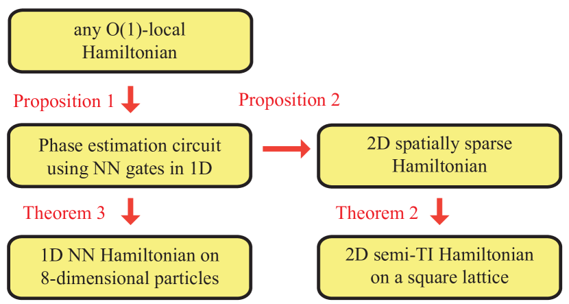
Figure 1: Overview of our constructions of 1D and 2D universal families of Hamiltonians. NN = nearest-neighbor.

Figure 1 explains the proof structure for constructing both the 2D and 1D universal Hamiltonians. The proofs diverge only after the first step, Proposition 1, in which the target Hamiltonian is replaces by a phase estimation circuit in 1D. The 1D and 2D cases differ in the way we map the resultant 1D circuit back to a Hamiltonian.

IV.2 The 1D phase estimation circuit: Proposition 1

We first show—and this is fairly standard—that one can construct a phase estimation circuit $U_{\rm PE}^{\textnormal{NN}}$ that would take eigenstates of $H$ as input and (approximately) write down their energy on ancilla qubits, using only nearest-neighbor gates acting on a line of qubits. Note that if $H$ is an $O(1)$-local $n$-qu$d$it Hamiltonian where $d$ is a constant, we can easily convert it to an $O(1)$-local $O(n)$-qubit Hamiltonian by simply encoding each qu$d$it in the subspace of a group of $\lceil\log_{2}d\rceil$ qubits. We can separate the extra states in this redundant encoding (when $d$ is not a power of 2) from the spectrum by adding to the Hamiltonian a local energy penalty term on each group with $\|H\|=O(\operatorname{poly}(n))$ magnitude. Hence, for simplicity of the discussion that follows, we will assume that this conversion is always performed first, and $H$ is an $O(1)$-local $n$-qubit Hamiltonian whose interaction energy is at most $O(\operatorname{poly}(n))$.

Given such a Hamiltonian $H$, let us write $H=\sum_{\mu}E_{\mu}|\psi_{\mu}\rangle\langle\psi_{\mu}|$ in its energy eigenbasis, where $0\leq E_{\mu}\leq E_{\max}$ without loss of generality. Note the upper bound $E_{\max}=O(\operatorname{poly}(n))$ can be computed without knowledge of the energy eigenvalues, e.g. by adding up the spectral norm of individual local terms of $H$.

Ideally, we want a phase estimation circuit $U_{\rm PE}^{\textnormal{ideal}}$ that acts on any input state of the form $\ket{\psi}\ket{0^{m}}=\sum_{\mu}c_{\mu}\ket{\psi_{\mu}}\ket{0^{m}}$ in the following way

$$U_{\rm PE}^{\textnormal{ideal}}\sum_{\mu}c_{\mu}\ket{\psi_{\mu}}\ket{0^{m}}=\sum_{\mu}c_{\mu}\ket{\psi_{\mu}}\ket{E_{\mu}},$$ (3)

where the first $s=O(\log(n))$ qubits of the $m$-qubit ancilla register encodes the energy $E_{\mu}$ as $\ket{E_{\mu}}=\ket{\varphi_{1}\varphi_{2}\dots\varphi_{s}}\otimes\ket{\text{rest}_{\mu}}$. Here, $\varphi_{\mu}=0.\varphi_{1}\varphi_{2}\dots$ is the binary representation of the real number $\varphi_{\mu}=E_{\mu}/E_{\max}$.

Nevertheless, we want to implement $U_{\rm PE}^{\textnormal{ideal}}$ with only polynomial number of local gates, which can be done using the Trotter decomposition Trotter (1959). We also want to use a discrete set of 2-qubit universal gates, which can be done by invoking the Solovay-Kitaev theorem Dawson and Nielsen (2006). This gives us $U_{\textnormal{PE}}^{\textnormal{local}}$, which will have some error $\zeta=\|(U_{\textnormal{PE}}^{\textnormal{local}}-U_{\rm PE}^{\textnormal{ideal}})\ket{\psi}\ket{0^{m}}\|$. This error $\zeta$ can be made small using only $O(\operatorname{poly}(n,\zeta^{-1}))$ resources (see Appendix A). Then, as shown in Fig. 2(a), we make all gates to be nearest-neighbor on a line by adding swap gates, obtaining $U_{\textnormal{PE}}^{\textnormal{NN}}$. This fact is summarized as Proposition 1:

Proposition 1.

Given any $n$-qubit $O(1)$-local Hamiltonian $H=\sum_{\mu}E_{\mu}|\psi_{\mu}\rangle\langle\psi_{\mu}|$, one can construct a circuit $U_{\textnormal{PE}}^{\textnormal{NN}}$ consisting of $\operatorname{poly}(n,\zeta^{-1})$ gates acting on $n+m$ qubits with 1- or 2-qubit nearest-neighbor gates chosen from a universal gate set, where $m=\operatorname{poly}(n)$, such that for any normalized input state $\sum_{\mu}c_{\mu}\ket{\psi_{\mu}}$

$$\Big{\|}U_{\textnormal{PE}}^{\textnormal{NN}}\sum_{\mu}c_{\mu}\ket{\psi_{\mu}}\ket{0^{m}}-\sum_{\mu}c_{\mu}\ket{\psi_{\mu}}\ket{E_{\mu}}\Big{\|}\leq\zeta$$ (4)

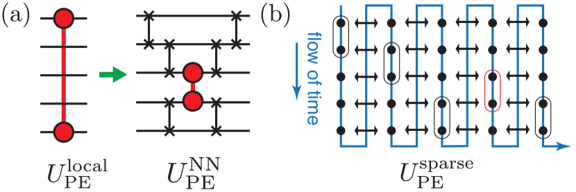
Figure 2: Illustration of converting a circuit to a spatially sparse one. (a) Adding swap gates to make a 2-qubit gate (red) acting on distant qubits nearest-neighbor. (b) Adding new qubits so that the execution of gates are in a spatially local sequence.

IV.3 Constructing 2D semi-TI strongly universal Hamiltonians

To prove Theorem 2, we want to simulate any local Hamiltonian $H$ with a $\mathcal{S}$-Hamiltonian on a 2D square lattice with polynomial overhead, for any non-2SLD $\mathcal{S}$. We start by first constructing a spatially sparse circuit Hamiltonian $H_{\textnormal{circuit}}$ that simulates our original target Hamiltonian $H$ (Proposition 2). Then the (semi-translation-invariant) $\mathcal{S}$-Hamiltonian simulator on the 2D lattice is obtained from $H_{\textnormal{circuit}}$ by applying a series of gadgets. The full technical proof in given in Appendix B, but we will sketch the essential ideas below. To that end, we borrow the notion of spatial sparsity from Ref. Oliveira and Terhal (2008); Cubitt et al. (2018) and generalize it to circuits:

Definition 6 (Spatial sparsity of Hamiltonians and circuits (adapted from Oliveira and Terhal (2008))).

A Hamiltonian on $n$-qudits is spatially sparse if its interaction hypergraph is one where (i) every vertex participates in $O(1)$ hyper-edges, and $(ii)$ there is a straight-line drawing in the plane such that every hyper-edge overlaps with $O(1)$ other hyper-edges, and the surface covered by every hyper-edge is $O(1)$. Moreover, we say a quantum circuit $U=\prod_{t=1}^{T}U_{t}$ is spatially sparse if there is a placement of the qudits in the two-dimensional plane such that (i) each qudit participates in $O(1)$ gates, and (ii) the spatial supports of $U_{t}$ and $U_{t+1}$ are only $O(1)$ distance apart for all $t$, each covering $O(1)$ contiguous area.

With the definition of spatial sparsity in hand, we now formally state the Proposition we want to show:

Proposition 2.

Given any $O(1)$-local $n$-qudit Hamiltonian $H$ with $\|H\|=O(\operatorname{poly}(n))$, one can construct a spatially sparse $5$-local Hamiltonian $H_{\textnormal{circuit}}$ that efficiently simulates $H$ to precision $(\Delta,\eta,\epsilon)$, with $\Delta=O(\epsilon^{-1}\|H\|^{2}+\eta^{-1}\|H\|)$. $H_{\textnormal{circuit}}$ has $O(\operatorname{poly}(n,\epsilon^{-1}))$ terms and qubits, and interaction energy at most $O(\operatorname{poly}(n,\eta^{-1},\epsilon^{-1}))$.

To prove this Proposition, we start from the 1D phase estimation circuit obtained using Proposition 1 and construct a spatially sparse circuit using swap gates. To do this, we first make $U_{\textnormal{PE}}^{\textnormal{NN}}$ spatially sparse into $U_{\rm PE}^{\text{sparse}}$ by moving it from the line to a 2D grid. As visualized in Fig. 2(b), starting from the leftmost column of qubits, we apply just one nearest-neighbor gate before swapping all qubits to the next column and applying the next gate, getting us $U_{\rm PE}^{\rm sparse}$. By ordering the gates in a snake-like fashion similar to Ref. Aharonov et al. (2007); Oliveira and Terhal (2008), we make sure that each qubit participates in only a constant number of gates, and that the temporally proximate gates in the sequence have spatially proximate support.

Before converting the circuit back to a Hamiltonian, we need to address the issue of the entanglement between each energy eigenstate and the ancilla register that has the energy bit-string, as evident in Eq. (3). This incoherence between different eigenstates causes a large error for the simulation if left unchecked. We repair this error by running the circuit backwards (“uncomputing”) and then adding $L$ identity gates at the end (“idling”), so that most of the computational history of each eigenstate is simply the state itself. We then get a new circuit which $U_{\textnormal{circuit}}=(\mathds{1})^{L}(U_{\textnormal{PE}}^{\textnormal{sparse}})^{\dagger}(\mathds{1})^{s}U_{\textnormal{PE}}^{\textnormal{sparse}}$, which is spatially sparse as long as $U_{\textnormal{PE}}^{\textnormal{sparse}}$ is. Note we inserted $s$ identity gates before applying $(U_{\textnormal{PE}}^{\textnormal{sparse}})^{\dagger}$ so that we can examine the energy bit-string bit-by-bit before it is uncomputed.

Subsequently, we apply Kitaev’s circuit-to-Hamiltonian mapping Kitaev et al. (2002) to convert the spatially sparse, “uncomputed” circuit $U_{\textnormal{circuit}}$ to a spatially sparse Hamiltonian $H_{\textnormal{circuit}}$. The energy of the eigenstates of $H$ are restored by adding an appropriate bit-wise energy penalty on the $s$ qubits where the energy is written, while we idle between $U_{\textnormal{PE}}^{\textnormal{sparse}}$ and $(U_{\textnormal{PE}}^{\textnormal{sparse}})^{\dagger}$ [see Eq. (21)]. We then use perturbative argument (such as those shown in Ref. Bravyi and Hastings (2014)) to show that $H_{\textnormal{circuit}}$ simulates $H$ with polynomially small error, with only polynomial overheads. This proves Proposition 2.

Finally, to prove Theorem 2, we map the spatially sparse Hamiltonian $H_{\textnormal{circuit}}$ to a Hamiltonian in a universal family on the 2D square lattice with additional polynomial overhead. This is done via a sequence of reductions, with known techniques Oliveira and Terhal (2008); Cubitt et al. (2018): We first converted $H_{\textnormal{circuit}}$ to a real-valued Hamiltonian by doubling the number of qubits, and encoding any Pauli $Y$’s into a pair of $Y\otimes Y$. We then remove all Pauli $Y$’s, and reduce the locality of the Hamiltonian to 2-local via applications of perturbative gadgets. This is subsequently converted to a spatially sparse $\mathcal{S}_{0}$-Hamiltonian where $\mathcal{S}_{0}=\{XX+YY+ZZ\}$ or $\{XX+YY\}$. Throughout this sequence of reductions, the spatial sparsity of the Hamiltonian is preserved, and both the interaction energy and qubit number only increases polynomially as the original system size and the target precision parameters $(\Delta,\eta,\epsilon)$. This spatially sparse $\mathcal{S}_{0}$-Hamiltonian involving only Pauli-interactions without $Y$’s can then be mapped to a $\mathcal{S}_{0}$-Hamiltonian on the 2D lattice. Since the input Hamiltonian is spatially sparse, this mapping only incurs polynomial overhead in the interaction energy as shown in Ref. Oliveira and Terhal (2008); Cubitt et al. (2018). Furthermore, Ref. Cubitt et al. (2018) has shown that $\mathcal{S}_{0}$-Hamiltonian on a 2D square lattice can be simulated by any $\mathcal{S}$-Hamiltonian on a 2D square lattice for any non-2SLD $\mathcal{S}$, with polynomial overhead. We have thus provided a construction that allows any such family of $\mathcal{S}$-Hamiltonians on the 2D square lattice to efficiently simulate any local Hamiltonian with arbitrary geometry.

IV.4 Constructing 1D universal Hamiltonians

We now show how to construct a strongly universal family of Hamiltonian simulators in 1D. To prove this result as stated in Theorem 3, we extend the circuit-to-1D-Hamiltonian constructions in Ref. Aharonov et al. (2009); Hallgren et al. (2013). These constructions were originally used to show QMA-completeness of Hamiltonians involving nearest-neighbor interaction on a 1D line of particles, by using them to encode the outcome of any circuit computation in their ground state energy.

The basic idea in these constructions is as follows. Suppose we are given any quantum circuit consisting of $R$ rounds of nearest-neighbor gates on $n$ qubits in 1D such as $U_{\textnormal{PE}}^{\textnormal{NN}}$, where each round is of the form $U_{n-1,n}\cdots U_{23}U_{12}$ (some may be identity). We consider an equivalent circuit on a line of $2nR$ particles, divided into $R$ blocks, where each block encodes the computational state of the original $n$ qubits. In this equivalent circuit, a single round of nearest-neighbor gate is applied in each block before the qubits are moved to the next block where subsequent gates can be performed. The 8 internal dimensions of each particle are necessary to store both the computational state of the original qubit and marker states that allows us to locally distinguish different stages of the computation of each particle (e.g., whether a gate has already been applied or needs to be applied).

We want to apply these constructions to simulate general Hamiltonians. Following the same idea as in the proof of Theorem 2, we first convert the target Hamiltonian $H$ to a phase estimation circuit $U_{\textnormal{PE}}^{\textnormal{NN}}$ using nearest-neighbor gates on a line of qubits as in Proposition 1. Then, we use the method in Ref. Hallgren et al. (2013) as well as our tricks of “uncomputing” and “idling” to map the circuit to a 1D Hamiltonian of nearest neighbor-interactions, and penalize the energy bit-string so that we simulate the full spectral properties of $H$. However, a naïve application of this method would yield a highly non-local encoding, since the idling part of the circuit corresponds to simply move the computational qubits down the line, causing the encoded eigenstates of $H$ to be delocalized over many blocks of particles. To circumvent this issue, we modified the method so that the idling step is done without moving the computational qubits, while maintaining the consistency of all transition rules so that the legal computational history states are spectrally gapped from the rest. Consequently, the eigenstates of $H$ are encoded in the qubit-subspace of some 8-dimensional qudits from just one block of the line, yielding a local encoding. For the full proof with technical details, see Appendix C.

In this construction, our 1D simulator does not have any form of translation-invariance, since its nearest-neighbor terms vary from block to block where different gates from $U_{\textnormal{PE}}^{\textnormal{NN}}$ are applied. Note the semi-translation-invariance in our 2D simulator is achieved (as done in Refs. Cubitt et al. (2018); Piddock and Montanaro (2018); Piddock and Bausch (2020)) using gadgets to simulate general interactions with a single type of interaction. Since these gadgets require ancilla particles placed in more than one dimension, it appears we cannot apply them to make our 1D construction semi-translation-invariant.

V Discussion

We have significantly improved the prospects of universal analog quantum simulation by showing that a strong notion of universality is possible with simple families of Hamiltonians embedded in constant dimensions. Unlike previous works Cubitt et al. (2018); Piddock and Montanaro (2018); Piddock and Bausch (2020); Kohler et al. (2020), our results show that only polynomial overheads in both particle number and interaction energy are sufficient to simulate any local Hamiltonian with arbitrary connectivity by some universal Hamiltonians embedded in 1D or 2D. Our results are tight in the sense that the overhead in the interaction energy cannot be brought down to a constant using constant-dimensional Hamiltonian simulators, due to an earlier result Aharonov and Zhou (2019) that gave counterexamples showing such simulations are impossible. We remark that even though there are weakly universal, fully translation-invariant families of Hamiltonians Piddock and Bausch (2020); Kohler et al. (2020), the interaction energy in those Hamiltonians has to scale exponentially with the size of the target Hamiltonian, since the target Hamiltonian’s spectrum is encoded in an exponentially vanishing fraction of the spectrum of the simulator.

An interesting open question is: Are there are strongly universal semi-translation-invariant Hamiltonians in 1D? Since the known gadgets to simulate general interactions with a single type of interaction seem to require ancilla particles placed in more than one dimension, we would likely need to invent new gadgetry.

We can also ask if there are strongly universal Hamiltonians with full translation-invariance in any constant dimensions. This is impossible if translation-invariance is required in the strongest sense, where the only free parameter of the Hamiltonians is the number of particle $n^{\prime}$; since such Hamiltonians can be described by $O(\log n^{\prime})$ bits of information, they cannot represent general Hamiltonians on $n$ qudits that are described by $\operatorname{poly}(n)$ bits unless $n^{\prime}=\exp(\operatorname{poly}(n))$. Indeed, Refs. Piddock and Bausch (2020); Kohler et al. (2020) constructed such families of Hamiltonians that are weakly universal, but cannot be strongly universal. This implies that there not all weakly universal families are strongly universal. To move towards full-TI strong universality, we may consider relaxing the notion of simulation: for example, Ref. Bohdanowicz and Brandão (2017) constructed a 1D fully translation-invariant family of Hamiltonians that can simulate any Hamiltonian by allowing for polynomial-sized encoding and decoding circuits. However, the desirable properties of analog Hamiltonian simulations such as preserving locality of observables and noise will no longer hold once we have encoding circuits that induce non-local correlations. Alternatively, one can consider relaxing translation-invariance by letting Hamiltonian interactions have more free parameters to encode the target Hamiltonian. Ref. Kohler et al. (2020) has done this to keep the number of particles in the simulator $O(\operatorname{poly}(n))$, but their construction still requires exponential overhead in the interaction energy. Nevertheless, it is likely possible to efficiently simulate any full-TI Hamiltonian by a family of full-TI Hamiltonian, where the description of both Hamiltonians are $O(\log n)$ bits. It would be worthwhile to investigate whether these constructions can be improved, or show that strong universality of full-TI Hamiltonians is impossible.

While this work has established that efficient universal analog quantum simulation using simple 1D or 2D systems is possible, the constructions we have provided here is far from optimal. Although we have shown that resources scaling only polynomially in the target system size are sufficient for analog simulation of any local Hamiltonian, there is much room for improvement in the scaling for practical applications. As experimental realizations of analog quantum simulators develop rapidly, we hope our work provides a starting point for researchers to develop methods to expand their scope to simulate all physical systems and tackle classically intractable problems.

Appendix A A 1D nearest-neighbor implementation of phase estimation circuit

In this appendix, we show that given any local Hamiltonian $H$, how to construct a phase estimation circuit such that the energy of any input eigenstate of $H$ can be written down as bits on some ancilla qubits to $O(\log n)$ bit precision with $O(1/\operatorname{poly}(n))$ error in the state. In particular, we show that this can be done with a circuit acting on a line of qubits with nearest-neighbor gates. This will serve as the backbone of our efficient construction of universal Hamiltonian simulators.

Proposition 1 (formal).

Consider any $O(1)$-local Hamiltonian $H=\sum_{a}H_{a}=\sum_{\mu}E_{\mu}|\psi_{\mu}\rangle\langle\psi_{\mu}|$ acting on $n$ qubits, where we assume w.l.o.g. that $0\leq E_{\mu}\leq E_{max}$ for some known number $E_{max}=O(\operatorname{poly}(n))$. For any $s=O(\log n)$ and $\zeta>0$, we can construct a phase estimation circuit $U_{\textnormal{PE}}^{\textnormal{NN}}$ consisting of $O(\operatorname{poly}(n,\zeta^{-1}))$ 1- or 2-qubit nearest neighbor gates drawn from any universal gate set, acting on a line of $n+m$ qubits, where $m=O(\operatorname{poly}(n))$. For any normalized state $\sum_{\mu}c_{\mu}\ket{\psi_{\mu}}$, the circuit $U_{\textnormal{PE}}^{\textnormal{NN}}$ satisfies

$$\left\|U_{\textnormal{PE}}^{\textnormal{NN}}\sum_{\mu}c_{\mu}\ket{\psi_{\mu}}\ket{0^{m}}-\sum_{\mu}c_{\mu}\ket{\psi_{\mu}}\ket{\tilde{E}_{\mu}}\ket{\textnormal{rest}_{\mu}}\right\|\leq\zeta$$ (5)

where $\ket{\tilde{E}_{\mu}}=\ket{\varphi_{\mu,1}\varphi_{\mu,2}\varphi_{\mu,3}\cdots\varphi_{\mu,s}}$ is the $s$-bit truncated representation of $\varphi_{\mu}=E_{\mu}/E_{max}=0.\varphi_{\mu,1}\varphi_{\mu,2}\varphi_{\mu,3}\cdots$ with $\varphi_{\mu,j}\in\{0,1\}$, and $\ket{\textnormal{rest}_{\mu}}$ is some unimportant state on the remaining ancilla qubits.

Proof.

Let us first consider the standard implementation of quantum phase estimation algorithm circuit $U_{\textnormal{PE}}$. Here, the circuit uses the evolution operator $u_{j}=e^{iH\tau 2^{j-1}}$ under $H$, where $\tau=2\pi/E_{max}$, and writes phase of the eigenvalues of $u_{1}=e^{iH\tau}$ on some ancilla qubits. Note the eigenvalues of $u_{1}$ are $e^{i2\pi\varphi_{\mu}}$, where $\varphi_{\mu}=E_{\mu}\tau/(2\pi)$. Since $0\leq\varphi_{\mu}\leq 1$, we can write $\varphi_{\mu}=0.\varphi_{\mu,1}\varphi_{\mu,2}\varphi_{\mu,3}\cdots$.

Ideally, the action of the phase estimation circuit on input states $\{\ket{\psi_{\mu}}\ket{0^{m}}\}_{\mu=1}^{2^{n}}$ is

$$U_{\rm PE}^{\textnormal{ideal}}\ket{\psi_{\mu}}\ket{0^{m}}=\ket{\psi_{\mu}}\ket{\tilde{E}_{\mu}}\ket{\textnormal{rest}_{\mu}},$$ (6)

Correspondingly, let us denote $\tilde{E}_{\mu}=2\pi\tilde{\varphi}_{\mu}/\tau$ as approximate values of the energy $E_{\mu}$, where $\tilde{\varphi}_{\mu}=0.\varphi_{\mu,1}\varphi_{\mu,2}\varphi_{\mu,3}\cdots\varphi_{\mu,s}$. In the ideal case, $E_{\mu}=\tilde{E}_{\mu}$ for some sufficiently large $s$.

In reality, there are two sources of errors that cause the phase estimation circuit to deviate from $U_{\rm PE}^{\textnormal{ideal}}$.

Error 1: finite-bit-precision— The first is due to the fact that the energy eigenvalues don’t generally have finite-bit-precision representation, i.e., $|E_{\mu}-\tilde{E}_{\mu}|=O(2^{-s})$ is non-zero. In other words, since $\varphi_{\mu}\neq\tilde{\varphi}_{\mu}$, there’s additional error from imprecise phase estimation. Let us consider a phase estimation circuit $U_{\rm PE}$ implemented to $p$-bit precision, where $p>s$. Let $b_{\mu}$ be the integer in the range $[0,2^{p}-1]$ such that $0\leq\varphi_{\mu}-b_{\mu}/2^{p}\leq 2^{-p}$. It is well-known Nielsen and Chuang (2011) that the action of $U_{\rm PE}$ on any input state $\ket{\psi_{\mu}}\ket{0}$ result in the following state

$$U_{\rm PE}\ket{\psi_{\mu}}\ket{0^{m}} =\ket{\psi_{\mu}}\ket{\textnormal{rest}_{\mu}^{\prime}}\otimes\frac{1}{2^{p}}\sum_{k,\ell=0}^{2^{p}-1}e^{-i2\pi k\ell/2^{p}}e^{i2\pi\varphi_{\mu}k}\ket{\ell}=\ket{\psi_{\mu}}\ket{\textnormal{rest}_{\mu}^{\prime}}\sum_{\ell=0}^{2^{p}-1}\alpha_{\ell}^{\mu}\ket{\ell}$$ (7)

where $\ket{\ell}=\ket{\ell_{1}\cdots\ell_{p}}$ is the binary representation of $\ell$, and

$$\alpha_{\ell}^{\mu} =\frac{1}{2^{p}}\sum_{k=0}^{2^{p}-1}[e^{i2\pi(\varphi_{\mu}-\ell/2^{p})}]^{k}=\frac{1}{2^{p}}\left[\frac{1-e^{i2\pi(2^{s}\varphi_{\mu}-\ell)}}{1-e^{i2\pi(\varphi_{\mu}-\ell/2^{p})}}\right]$$ (8)

The analysis from Sec. 5.2.1 in Ref. Nielsen and Chuang (2011) shows that the probability of getting a state that is a distance of $e$ integer away is

$$p_{\mu}^{\text{error}}(e)\equiv\sum_{|\ell-b_{\mu}|>e}|\alpha_{\ell}^{\mu}|^{2}\leq\frac{1}{2(e-1)}$$ (9)

Note that we only care about the first $s<p$ bits, so we can choose $e=2^{p-s}-1$.Hence,

$$U_{\rm PE}\ket{\psi_{\mu}}\ket{0^{m}} =\ket{\psi_{\mu}}\ket{\textnormal{rest}_{\mu}^{\prime}}\otimes\left[\sum_{|\ell-b_{\mu}|\leq e}\alpha_{\ell}^{\mu}\ket{\ell}+\sum_{|\ell-b_{\mu}|>e}\alpha_{\ell}^{\mu}\ket{\ell}\right]$$

$$=\ket{\psi_{\mu}}\ket{\textnormal{rest}_{\mu}^{\prime}}\otimes\left(\sqrt{1-p_{\mu}^{\text{error}}}\ket{\tilde{E}_{\mu}}\ket{\textnormal{rest}^{1}_{\mu}}+\sqrt{p_{\mu}^{\text{error}}}\ket{\textnormal{rest}^{2}_{\mu}}\right)$$ (10)

Comparing this with the idealized output in Eq. (6), we can identify $\ket{\textnormal{rest}_{\mu}}=\ket{\textnormal{rest}_{\mu}^{\prime}}\ket{\textnormal{rest}_{\mu}^{1}}$, and observe that

$$(U_{\rm PE}-U_{\rm PE}^{\textnormal{ideal}})\ket{\psi_{\mu}}\ket{0^{m}}=\ket{\psi_{\mu}}\ket{\text{error}_{\mu}},\quad\text{where}\quad\left\|\ket{\text{error}_{\mu}}\right\|^{2}\leq 2p^{\text{error}}_{\mu}=O(2^{-(p-s)})$$ (11)

Thus, for any normalized state $\ket{\psi}=\sum_{\mu}c_{\mu}\ket{\psi_{\mu}}\ket{0^{m}}$, we have

$$\|(U_{\rm PE}-U_{\rm PE}^{\textnormal{ideal}})\sum_{\mu}c_{\mu}\ket{\psi_{\mu}}\ket{0^{m}}\|^{2}=O(2^{-(p-s)})\leq O(\zeta)$$ (12)

where we chose, for example, $p=2s+O(\log\zeta^{-1})$ and $s=O(\log(n))$, and thus make this first source of error due to imprecision to be smaller than any constant $c_{1}$.

Error 2: local gate approximation of $e^{-iH\tau_{j}}$— The second source of error is due to the fact that we need to implement the circuit $U_{\textnormal{PE}}$ using only 1 or 2-qubit gates, in order to ensure the corresponding circuit-Hamiltonian is local, The only non-local gates in the $p$-bit precise phase estimation algorithm that we need to address are the controlled-application of Hamiltonian evolution, $|0\rangle\langle 0|\otimes\mathds{1}+|1\rangle\langle 1|\otimes u_{j}$, where $u_{j}=e^{-iH\tau_{j}}$, $\tau_{j}=2^{j-1}\tau$ and $j=1,2,\ldots,p$. This can be implemented with local gates via Trotter decomposition Trotter (1959).

Specifically, we write $H=\sum_{a=1}^{M_{0}}H_{a}$, where $H_{a}$ is a $k$-local term, and $M_{0}=O(\operatorname{poly}(n))$ is the number of terms. We can implement $\tilde{u}_{j}=(\prod_{a=1}^{M_{0}}e^{-iH_{a}\tau_{j}/r_{j}})^{r_{j}}$ for some integer $r_{j}$, so that $\|\tilde{u}_{j}-u_{j}\|\leq O(\tau_{j}^{2}/r_{j})$. Since $p=O(\log n+\log\zeta^{-1})$, we have $\tau_{j}=O(2^{p}/\|H\|)=O(\operatorname{poly}(n,\zeta^{-1}))$. We can then choose $r_{j}=O(\tau_{j}^{2}\operatorname{poly}(\zeta^{-1}))=O(\operatorname{poly}(n,\zeta^{-1}))$ to ensure each such error is polynomially small. The error from Trotter decomposition is bounded by

$$\|U_{\rm PE}^{\rm Trot}-U_{\rm PE}\|\leq\sum_{j=1}^{p}O(\tau_{j}^{2}/r_{j})\leq O(\zeta)$$ (13)

The total number of local gates in $U_{\textnormal{PE}}^{\rm Trot}$ is $R_{\rm Trot}=O(M_{0}\sum_{j}r_{j})=O(\operatorname{poly}(n,\zeta^{-1}))$, and the locality of each gate is at most $k+1$.

We still need a circuit with only 1- or 2-qubit gates drawn from a universal set of gates. To that end, we can apply the Solvay-Kitaev algorithm to approximate each $(k+1)$-local gate with a sequence of 2-local gates. It is knownDawson and Nielsen (2006) that to approximate any gate in $SU(d)$ with 2-local gates to $\epsilon_{0}$-precision, we’ll need at most $O(d^{2}\operatorname{poly}\log\epsilon_{0}^{-1})$ 2-qubit gates from some universal gate set of finite size. Note $d=2^{k+1}$ when we are approximating $(k+1)$-local gates with 2-qubit gates. As there are at most $R_{\rm Trot}$ such gates, to keep the overall error to be below $O(\zeta)$, we only need $\epsilon_{0}\leq O(\zeta/R_{\rm Trot})=O(1/\operatorname{poly}(n,\zeta^{-1})))$. This means we need to approximate each $(k+1)$-local gates with $R_{\rm SK}=O(4^{k}\operatorname{poly}(\log n,\log\zeta^{-1}))$ 2-qubit gates. The final circuit is $U_{\textnormal{PE}}^{\textnormal{local}}$ consisting of only $R_{\textnormal{local}}=O(R_{\rm Trot}R_{\rm SK})=O(\operatorname{poly}(n,\zeta^{-1}))$ 1- or 2-qubit gates, for $k=O(1)$.

We can then ensure that this circuit $U_{\textnormal{PE}}^{\rm local}$ only consists of nearest-neighbor gates by the following procedure:

1. Place all $n$ qubits on a line with any pre-determined ordering.

2. Iterate over each gate $U_{t}$, $t=1,\ldots R_{\textnormal{local}}$. If $U_{t}$ acts on qubits that are not neighbors on the line, add a sequence $S_{t}$ of swap gates on nearest neighbors in the circuit before $U_{t}$ so that $U_{t}$ acts on neighbors. Then add the same swap gates in reversed order in the circuit after $U_{t}$ so that the qudits returned to their original order on the line. At the end of this step, the new circuit is of the form $U_{\rm PE}^{\rm NN}=\prod_{t=1}^{R_{0}}(S_{t}^{\dagger}U_{t}S_{t})$, with $R_{0}=O(R_{\textnormal{local}}N)$ gates, each only acting on a neighbors group of qubits. See Fig. 2(a) for an example.

Putting everything together, we have $U_{\textnormal{PE}}^{\textnormal{NN}}=U_{\textnormal{PE}}^{\textnormal{local}}\approx U_{\textnormal{PE}}^{\rm Trot}\approx U_{\textnormal{PE}}\approx U_{\textnormal{PE}}^{\textnormal{ideal}}$. In conclusion, for any $\zeta>0$, we can construct a phase estimation circuit $U_{\textnormal{PE}}^{\textnormal{NN}}$ comprised of only $O(\operatorname{poly}(n,\zeta^{-1}))$ 1-qubit or 2-qubit nearest-neighbor gates on a line, such that its action is $\zeta$-close to $U_{\rm PE}^{\textnormal{ideal}}$ on any valid input state $\sum_{\mu}c_{\mu}\ket{\psi_{\mu}}\ket{0^{m}}$:

$$\|(U_{\rm PE}^{\textnormal{NN}}-U_{\rm PE}^{\textnormal{ideal}})\ket{\psi}\ket{0^{m}}\|\leq\zeta.$$ (14)

∎

Appendix B Proof that spin models on 2D lattice is strongly universal

In this section, we show the details of the construction for strongly universal Hamiltonian in 2D square lattice.

Theorem 2.

Any $\mathcal{S}$-Hamiltonian on the 2D square lattice is strongly universal, as long as $\mathcal{S}$ is non-2SLD. In particular, it’s sufficient for $\mathcal{S}$ to contain only a single interaction (such Heisenberg or XY-interaction), implying that there are semi-translation-invariant Hamiltonians in 2D that are strongly universal.

B.1 Efficient, spatially sparse Hamiltonian simulator

Before proving the strong universality of 2D spin-lattice models, we first prove the following result, where we show that any local Hamiltonian can be simulated by a spatially sparse Hamiltonian.

Proposition 2.

Given any $O(1)$-local $n$-qudit Hamiltonian $H$ with $\|H\|=O(\operatorname{poly}(n))$, one can construct a spatially sparse $5$-local Hamiltonian $H_{\textnormal{circuit}}$ that efficiently simulates $H$ to precision $(\Delta,\eta,\epsilon)$, with $\Delta=O(\epsilon^{-1}\|H\|^{2}+\eta^{-1}\|H\|)$. $H_{\textnormal{circuit}}$ has $O(\operatorname{poly}(n,\epsilon^{-1}))$ terms and qubits, and interaction energy at most $O(\operatorname{poly}(n,\eta^{-1},\epsilon^{-1}))$.

To prove the above Proposition, we first prove two smaller Lemmas 1 and 2 about different aspects of using the Feynman-Kitaev circuit-to-Hamiltonian construction Kitaev et al. (2002) for Hamiltonian simulation. The following concept of history states will be useful in the discussion:

Definition 7 (history states).

Let $U=U_{T}\cdots U_{2}U_{1}$ be a quantum circuit acting on $n+m$ qudits. Then for any input state $\ket{\psi_{\mu}}\in\mathds{C}^{d^{n}}$, the history state with respect to $U$ and $\ket{\psi_{\mu}}$ is the following

$$\ket{\eta_{\mu}}=\frac{1}{\sqrt{T+1}}\sum_{t=0}^{T}\Big{(}U_{t}\cdots U_{2}U_{1}\ket{\psi_{\mu}}\ket{0^{m}}^{\textnormal{anc}}\Big{)}\ket{1^{t}0^{T-t}}^{\textnormal{clock}}$$ (15)

We now prove the first of the two Lemmas, which describes a circuit-to-Hamiltonian transformation that can be used for analog Hamiltonian simulation, assuming an appropriate energy penalty Hamiltonian $H_{out}$ can be constructed.

Lemma 1 (Circuit-Hamiltonian simulation).

Consider an orthonormal basis of states $\{\ket{\psi_{\mu}}\}_{\mu=1}^{d^{n}}$ on $n$ qudits. Let $U=\prod_{t=1}^{T}U_{t}$ be a quantum circuit where each gate $U_{t}$ is at most $k$-local. Let $\mathcal{L}=\operatorname{span}\{\ket{\eta_{\mu}}\}_{\mu=1}^{d^{n}}$ be the subspace of history states with respect to $U$ and $\{\ket{\psi_{\mu}}\}$, and let $H$ be any Hamiltonian. Suppose there exists a Hamiltonian $H_{out}$ such that

$$\|VHV^{\dagger}-H_{out}|_{\mathcal{L}}\|\leq\epsilon/2$$ (16)

where $\mathcal{E}(H)=VHV^{\dagger}$ is a local encoding, and $O|_{\mathcal{L}}$ means operator $O$ restricted to subspace $\mathcal{L}$. Then for any $\eta>0$, we can construct a Hamiltonian $H_{\textnormal{circuit}}$ from the description of $U$ such that $H_{\textnormal{circuit}}$ is a $(\Delta,\eta,\epsilon)$-simulation of $H$ with local encoding $\mathcal{E}$, where $\Delta\geq O(\epsilon^{-1}\|H_{out}\|^{2}+\eta^{-1}\|H_{out}\|)$, per Def. 2. The constructed ${H}_{\textnormal{circuit}}$ is $(k+3)$-local, has $O(T)$ terms and particles, and uses $O(\operatorname{poly}(n,T,\Delta))$ interaction energy. Furthermore, $H_{\textnormal{circuit}}$ is spatially sparse if the circuit $U$ is spatially sparse.

Lemma 2 (Idling to enhance simulation precision).

Consider an uncomputed quantum circuit $U_{D}\cdots U_{1}=\mathds{1}$. Suppose we add $L$ identity gates to the end of the circuit, so that we obtain a new circuit $U=\mathds{1}^{L}U_{D}\cdots U_{1}$ with length $T=D+L$. Let $\ket{\eta_{\mu}}$ be the history state with respect to $U$ and $\ket{\psi_{\mu}}$. Suppose $H=\sum_{\mu}E_{\mu}|\psi_{\mu}\rangle\langle\psi_{\mu}|$ and $H_{\textnormal{eff}}=\sum_{\mu}E_{\mu}|\eta_{\mu}\rangle\langle\eta_{\mu}|$. For any $\epsilon>0$, if we choose $L=O(\frac{D\|H\|^{2}}{\epsilon^{2}})$, then there is an ancilla state $\ket{\alpha}$ such that $\|H\otimes|\alpha\rangle\langle\alpha|-H_{\textnormal{eff}}\|\leq\epsilon$.

We are now ready to prove our main Proposition 2:

Proof of Proposition 2.

Given any $O(1)$-local $n$-qu$d$it Hamiltonian where $d$ is a constant, we can easily convert it to an $O(1)$-local $O(n)$-qubit Hamiltonian by simply encoding each qu$d$it in the subspace of a group of $\lceil\log_{2}d\rceil$ qubits. We can separate the extra states in this redundant encoding (when $d$ is not a power of 2) from the relevant part of spectrum by adding to the Hamiltonian a local energy penalty term on acting each group with $\|H\|=O(\operatorname{poly}(n))$ magnitude. Hence, we will call $H$ the $O(1)$-local $n$-qubit Hamiltonian containing $O(\operatorname{poly}(n))$-strength interactions obtained after this conversion.

Let us denote the normalized eigenstates of $H$ as $\ket{\psi_{\mu}}$, with corresponding eigenvalues $E_{\mu}$. We assume they are ordered such that $E_{1}\leq E_{2}\leq E_{3}\leq\cdots\leq E_{2^{n}}$.

From Proposition 1, for any $s=O(\log n)$, we can construct a $\zeta$-approximate, $s$-bit precise phase estimation circuit $U_{\textnormal{PE}}^{\textnormal{NN}}$ such that it acts on a line of $N=O(\operatorname{poly}(n))$ qubits with $R_{0}=O(\operatorname{poly}(n,\zeta^{-1}))$ nearest-neighbor gates. We want to replace it with a spatially sparse circuit $U_{\textnormal{PE}}^{\text{sparse}}$ with $O(R_{0}N)$ qubits and gates (see Definition 6). This can be done with polynomial overhead in the same way as in Ref. Oliveira and Terhal (2008); Aharonov et al. (2007). We begin by placing the $N$ original qubits on the first column of a $N\times R_{0}$ grid of qubits. For column $i=1,2,\ldots,R_{0}$, we execute only the $i$-th gate from the circuit $U_{\textnormal{PE}}^{\textnormal{NN}}$, and other uninvolved qubits are acted on by identity gates. After each column, we swap the state of the qubit of column $i$ to $i+1$. We order the execution of all the gates such that the gates from $U_{\textnormal{PE}}^{\textnormal{NN}}$ and identity gates are executed top-to-bottom, and the swap gates between column are executed from bottom-to-up [see Fig. 2(b)]. It is thus easy to see that in this new circuit $U_{\textnormal{PE}}^{\text{sparse}}$, each qubit participates in at most 3 gates (up to two swap gates and a non-trivial gate), and the gate are executed in a spatially local sequence. Note the action of $U_{\textnormal{PE}}^{\text{sparse}}$ is equivalent to $U_{\textnormal{PE}}^{\textnormal{NN}}$ up to re-ordering of the qubits, since we’ve only added swap gates. Thus, Proposition 1 gives us

$$\left\|U_{\textnormal{PE}}^{\text{sparse}}\sum_{\mu}c_{\mu}\ket{\psi_{\mu}}\ket{0^{m}}-\sum_{\mu}c_{\mu}\ket{\psi_{\mu}}\ket{\tilde{E}_{\mu}}\right\|\leq\zeta$$ (17)

where $\ket{\tilde{E}_{\mu}}=\ket{\varphi_{\mu,1}\varphi_{\mu,2}\varphi_{\mu,3}\ldots\varphi_{\mu,s}}\otimes\ket{\textnormal{rest}_{\mu}}$ contains the $s$-bit truncated representation of $\varphi_{\mu}=E_{\mu}/E_{max}=0.\varphi_{\mu,1}\varphi_{\mu,2}\varphi_{\mu,3}\cdots$, and $E_{max}$ is the upper bound on the maximum energy of the target Hamiltonian $H$ used in the construction of $U_{\textnormal{PE}}^{\textnormal{NN}}$. Let

$$\tilde{E}_{\mu}=E_{max}\times(0.\varphi_{\mu,1}\varphi_{\mu,2}\varphi_{\mu,3}\ldots\varphi_{\mu,s})=E_{\mu}+O(E_{max}2^{-s})$$ (18)

be the truncated-approximation to the energy eigenvalue $E_{\mu}$.

The new spatially sparse circuit $U_{\textnormal{PE}}^{\text{sparse}}$ now has $t_{0}=O(R_{0}N)=O(\operatorname{poly}(n,\zeta^{-1}))$ gates. From this, we construct the following uncomputed, spatially sparse circuit

$$U_{\textnormal{circuit}}=(\mathds{1})^{L}U_{\rm PE}^{\text{sparse}{\dagger}}(\mathds{1})^{s}U_{\rm PE}^{\text{sparse}},$$ (19)

which we will transform into our spatially sparse Hamiltonian. Note we add $U_{\rm PE}^{\text{sparse}{\dagger}}$ for uncomputing and $s+L$ idling identity gates, making the entire circuit gate count $T=2t_{0}+s+L$. The $s$ identity gates are used for local measurements of energy to $s$-bit precision, and $L=O((2t_{0}+s)\|H\|^{2}/\epsilon^{2})=O(\operatorname{poly}(n,\zeta^{-1})/\epsilon^{2})$ identity gates are used to ensure $O(\epsilon)$ simulation precision as in Lemma 2. The history states with respect to eigenstate $\ket{\psi_{\mu}}$ of $H$ and this circuit are

$$\ket{\eta_{\mu}}=\frac{1}{\sqrt{T+1}}\sum_{t=0}^{T}\Big{(}U_{t}\cdots U_{2}U_{1}\ket{\psi_{\mu}}\ket{0^{m}}\Big{)}\ket{1^{t}0^{T-t}}$$ (20)

We can convert the circuit to a Hamiltonian ${H}_{\textnormal{circuit}}$ using the method described in Lemma 1, where $H_{out}$ is chosen to be

$$H_{out}=(T+1)E_{max}\sum_{b=1}^{s}2^{-b}|1\rangle\langle 1|_{b}^{\textnormal{anc}}\otimes P^{\textnormal{clock}}(t=t_{0}+b).$$ (21)

We also denote $P^{\textnormal{clock}}(t)=|110\rangle\langle 110|_{t-1,t,t+1}^{\textnormal{clock}}$, which projects onto legal clock states corresponding to time step $t$.

To show that ${H}_{\textnormal{circuit}}$ simulates the original Hamiltonian $H$, we first show that $H_{out}$ restricted to the subspace of history states $\mathcal{L}=\operatorname{span}\{\ket{\eta_{\mu}}:1\leq\mu\leq 2^{n}\}$ can be approximated by the following effective Hamiltonian

$$H_{\textnormal{eff}}=\sum_{\mu}E_{\mu}|\eta_{\mu}\rangle\langle\eta_{\mu}|.$$ (22)

Consider arbitrary states $\ket{\eta}\in\mathcal{L}$. We write $\ket{\eta}=\sum_{\mu}a_{\mu}\ket{\eta_{\mu}}$, and observe

$$\braket{\eta}{H_{out}}{\eta} =E_{max}\sum_{b=1}^{s}2^{-b}\left[\sum_{\nu}a_{\nu}^{*}\bra{\psi_{\nu}}\bra{0^{m}}\right]U_{\rm PE}^{\text{sparse}{\dagger}}|1\rangle\langle 1|_{b}U_{\rm PE}^{\text{sparse}}\left[\sum_{\mu}a_{\mu}\ket{\psi_{\mu}}\ket{0^{m}}\right]$$ (23)

Then using (17), we have

$$\braket{\eta}{H_{out}}{\eta} =E_{max}\sum_{b=1}^{s}2^{-b}\left[\sum_{\nu}a_{\nu}^{*}\bra{\psi_{\nu}}\bra{\tilde{E}_{\nu}}+\bra{\zeta}\right]|1\rangle\langle 1|_{b}\left[\sum_{\mu}a_{\mu}\ket{\psi_{\mu}}\ket{\tilde{E}_{\mu}}+\ket{\zeta}\right]$$ (24)

where $\ket{\zeta}$ is some residual state vector with $\|\ket{\zeta}\|\leq\zeta$. Hence

$$\left|\braket{\eta}{H_{out}-H_{\textnormal{eff}}}{\eta}\right| \leq\sum_{\mu}|a_{\mu}|^{2}|\tilde{E}_{\mu}-E_{\mu}|+2s\zeta E_{max}\leq\max_{\mu}|\tilde{E}_{\mu}-E_{\mu}|+2s\zeta E_{max}\leq(2^{-s}+2s\zeta)E_{max}$$ (25)

We can ensure this is always less than $\epsilon/4$ by choosing for example

$$s=\log_{2}(8E_{\max}/\epsilon)=O(\log n+\log\epsilon^{-1})\quad\text{and}\quad\zeta=\epsilon/(16sE_{\max})=O(1/\operatorname{poly}(n,\epsilon^{-1})).$$ (26)

Hence,

$$\left|\braket{\eta}{H_{out}-H_{\textnormal{eff}}}{\eta}\right|\leq\epsilon/4\quad\forall\ket{\eta}\in\mathcal{L}\quad\Longrightarrow\quad\|H_{\textnormal{eff}}-H_{out}|_{\mathcal{L}}\|\leq\epsilon/4$$ (27)

Furthermore, since we have added $L$ idling gates such that $\|H\otimes|\alpha\rangle\langle\alpha|-H_{\textnormal{eff}}\|\leq\epsilon/4$ for some ancilla state $\ket{\alpha}$ by Lemma 2, then together with (27) we have

$$\|H\otimes|\alpha\rangle\langle\alpha|-H_{out}|_{\mathcal{L}}\|\leq\epsilon/2.$$ (28)

Observe that we can rewrite $H\otimes|\alpha\rangle\langle\alpha|=VHV^{\dagger}$, where $V\ket{\psi}=\ket{\psi}\ket{\alpha}$ $\forall\ket{\psi}\in\mathds{C}^{2^{n}}$ is an isometry. Hence, by Lemma 1, for any $\eta>0$, the constructed ${H}_{\textnormal{circuit}}$ simulates $H$ to precision $(\Delta,\eta,\epsilon)$, where $\Delta=O(\epsilon^{-1}\|H_{out}\|^{2}+\eta^{-1}\|H_{out}\|)=O(\epsilon^{-1}\|H\|^{2}+\eta^{-1}\|H\|)$. Note that $H_{\textnormal{circuit}}$ is spatially sparse since $U_{\rm PE}^{\text{sparse}}$ is spatially sparse. Since $U_{\rm PE}^{\text{sparse}}$ contains at most 2-local gates, which means $H_{\textnormal{circuit}}$ is at most 5-local. Furthermore, $H_{\textnormal{circuit}}$ contains $O(T)=O(\operatorname{poly}(n,\zeta^{-1})/\epsilon^{2})=O(\operatorname{poly}(n,\epsilon^{-1}))$ terms (and qubits), with $O(\operatorname{poly}(n,T,\epsilon^{-1},\eta^{-1},\|H_{out}\|))=O(\operatorname{poly}(n,\eta^{-1},\epsilon^{-1}))$ interaction energy.

∎

To finish the proof, we just need to prove Lemma 1 and 2. We start with the proof of Lemma 1.

Proof of Lemma 1.

For a given circuit $U=U_{T}\cdots U_{2}U_{1}$, the corresponding circuit-Hamiltonian is

$$H_{\textnormal{circuit}} =H_{0}+H_{out}$$ (29)

$$\text{where}\quad H_{0} =J_{clock}H_{clock}+J_{prop}H_{prop}+J_{in}H_{in}$$ (30)

The role of $H_{0}$ is to isolate $\mathcal{L}=\operatorname{span}\{\ket{\eta_{\mu}}\}$ as its zero-energy groundspace separated by a large spectral gap $2\Delta$ from the rest of the eigenstates. Then $H_{out}$ is used recover the eigenvalue structrue of $H$ in the subspace $\mathcal{L}$, allowing $H_{\textnormal{circuit}}$ to simulate $H$.

Now we give the explicit form of the circuit-Hamiltonian. The first part of $H_{0}$ is

$$H_{clock}=\sum_{t=1}^{T-1}|01\rangle\langle 01|^{\textnormal{clock}}_{t,t+1},$$ (31)

which sets the legal state configurations in the clock register to be of the form $\ket{t}^{\textnormal{clock}}\equiv\ket{1^{t}0^{T-t}}^{\textnormal{clock}}$. Then, we simulate the state propagation under the circuit using

$$H_{prop} = \sum_{t=1}^{T}H_{prop,t},$$ (32)

$$\text{where}\quad H_{prop,t} = \mathds{1}\otimes|100\rangle\langle 100|^{\textnormal{clock}}_{t-1,t,t+1}-U_{t}\otimes|110\rangle\langle 100|^{\textnormal{clock}}_{t-1,t,t+1}$$

$$-U_{t}^{\dagger}\otimes|100\rangle\langle 110|^{\textnormal{clock}}_{t-1,t,t+1}+\mathds{1}\otimes|110\rangle\langle 110|^{\textnormal{clock}}_{t-1,t,t+1}\quad\text{for}\quad 1<t<T,$$

$$H_{prop,1} = \mathds{1}\otimes|00\rangle\langle 00|_{12}^{\textnormal{clock}}-U_{1}\otimes|10\rangle\langle 00|_{12}^{\textnormal{clock}}-U_{1}^{\dagger}\otimes|00\rangle\langle 10|_{12}^{\textnormal{clock}}+\mathds{1}\otimes|10\rangle\langle 10|_{12}^{\textnormal{clock}},$$

$$\text{and}\quad H_{prop,T} = \mathds{1}\otimes|10\rangle\langle 10|_{T-1,T}^{\textnormal{clock}}-U_{T}\otimes|11\rangle\langle 10|_{T-1,T}^{\textnormal{clock}}-U_{T}^{\dagger}\otimes|10\rangle\langle 11|_{T-1,T}^{\textnormal{clock}}+\mathds{1}\otimes|11\rangle\langle 11|_{T-1,T}^{\textnormal{clock}}.$$

These terms check the propagation of states from time $t-1$ to $t$ is correct. Now, we also need to ensure that the input states are valid, i.e. ancilla qudits are in the state $\ket{0^{m}}^{\textnormal{anc}}$ when $t=0$ (i.e., the clock register is $\ket{0^{T}}^{\textnormal{clock}}$). This can be done using

$$H_{in}=\sum_{i=1}^{m}(\mathds{1}-|0\rangle\langle 0|)_{i}^{\textnormal{anc}}\otimes|0\rangle\langle 0|^{\textnormal{clock}}_{t_{\min}(i)},$$ (33)

$$\text{where}\quad t_{\min}(i)=\min\{t:U_{t}\text{ acts nontrivially on ancilla qudit }i\}.$$

In other words, for each ancilla qudit $i$, $H_{in}$ penalizes the ancilla if it’s not in the state $\ket{0}$ before it is first used by the $t_{\min}(i)$-th gate. Note that ${H}_{\textnormal{circuit}}$ has $O(T)$ terms, each of which is most $(k+3)$-local when $U_{t}$ are $k$-local. If $U$ is spatially sparse, then it is easy to see that $H_{\textnormal{circuit}}$ is also spatially sparse.

Note that $H_{0}\mathcal{L}=0$. We then need to lower bound the spectral gap of $H_{0}$, i.e. $\lambda_{1}(H_{0}|_{\mathcal{L}^{\perp}})$, where $\lambda_{1}(H)$ denotes the lowest eigenvalue of $H$. To that end, let us denote the following subspaces:

$$\mathcal{S}_{clock} =\operatorname{span}\{\ket{\psi}\ket{y}\ket{1^{t}0^{T-t}}:\ket{\psi}\in\mathds{C}^{d^{n}}\text{ and }\ket{y}\in\mathds{C}^{d^{m}},0\leq t\leq T\},$$ (34)

$$\mathcal{S}_{prop} =\operatorname{span}\{\ket{\eta_{\mu},y}\equiv\frac{1}{\sqrt{T+1}}\sum_{t=0}^{T}\Big{(}U_{t}\cdots U_{2}U_{1}\ket{\psi}\ket{y}\Big{)}\ket{1^{t}0^{T-t}}:1\leq\mu\leq d^{n},0\leq y\leq d^{n-1}\}.$$ (35)

Note that $\mathcal{L}\subset\mathcal{S}_{prop}\subset\mathcal{S}_{clock}$. Let us denote $\tilde{A}=\mathcal{A}\cap\mathcal{L}^{\perp}$ for any subspace $\mathcal{A}$. Note $H_{clock}\mathcal{S}_{clock}=0$, $H_{prop}\mathcal{S}_{prop}=0$, $H_{in}\mathcal{L}=0$. We will use the following Projection Lemma 3:

Lemma 3 (Projection Lemma, adapted from Kempe et al. (2006)).

Let $H=H_{1}+H_{2}$ be sum of two Hamiltonians operating on some Hilbert space $\mathcal{S}_{0}=\mathcal{S}\oplus\mathcal{S}^{\perp}$. Assuming that $H_{2}$ has a zero-energy eigenspace $\mathcal{S}\subseteq\mathcal{S}_{0}$ so that $H_{2}\mathcal{S}=0$, and that the minimum eigenvalue $\lambda_{1}(H_{2}|_{\mathcal{S}^{\perp}})\geq J>2\|H_{1}\|$, then

$$\lambda_{1}(H_{1}|_{\mathcal{S}})-\frac{\|H_{1}\|^{2}}{J-2\|H_{1}\|}\leq\lambda_{1}(H)\leq\lambda_{1}(H_{1}|_{\mathcal{S}}).$$ (36)

In particular, if $J\geq K\|H_{1}\|^{2}+2\|H_{1}\|=O(K\|H_{1}\|^{2})$, we have $\lambda_{1}(H_{1}|_{\mathcal{S}})-\frac{1}{K}\leq\lambda_{1}(H)\leq\lambda_{1}(H_{1}|_{\mathcal{S}}).$ $\blacklozenge$

Applying the above Lemma successively to $H_{0}$, we obtain

$$\lambda_{1}(H_{0}|_{\mathcal{L}^{\perp}}) \geq\lambda_{1}\left[(J_{prop}H_{prop}+J_{in}H_{in})|_{\tilde{\mathcal{S}}_{clock}}\right]-\frac{1}{K}\qquad\text{if}\quad J_{clock}=O(K\|J_{prop}H_{prop}+J_{in}H_{in}\|^{2})$$ (37)

$$\geq\lambda_{1}\left[(J_{in}H_{in})|_{\tilde{\mathcal{S}}_{prop}}\right]-\frac{2}{K}\qquad\text{if}\quad J_{prop}/T^{2}=O(K\|J_{in}H_{in}\|^{2})$$ (38)

where we used the fact that $\lambda_{1}(H_{clock}|_{\mathcal{S}_{clock}^{\perp}})\geq 1$, and $\lambda_{1}(H_{prop}|_{\mathcal{S}_{prop}^{\perp}})\geq c/T^{2}$ for some constant $c$. We now lower bound (38). Let us denote $\hat{n}=\mathds{1}-|0\rangle\langle 0|$. Then within $\mathcal{S}_{clock}$, we can rewrite

$$H_{in}|_{\mathcal{S}_{clock}} =\sum_{i=1}^{m}\hat{n}_{i}^{\textnormal{anc}}\otimes\sum_{0\leq t\leq t_{\min}(i)}|t\rangle\langle t|^{\textnormal{clock}}=\sum_{t=0}^{\max_{i}t_{\min}(i)}H_{in,t}$$ (39)

$$\text{where}\quad H_{in,t} =\sum_{\{i:~{}t\leq t_{\min}(i)\}}\hat{n}_{i}^{\textnormal{anc}}\otimes|t\rangle\langle t|^{\textnormal{clock}}.$$

In particular, $H_{in,t=0}=\sum_{i=1}^{m}\hat{n}_{i}^{\textnormal{anc}}\otimes|t=0\rangle\langle t=0|$. Thus, for any $\ket{\eta_{\mu},y},\ket{\eta_{\nu},y^{\prime}}\in\tilde{\mathcal{S}}_{prop}$, where necessarily $y,y^{\prime}>0$, we have

$$\braket{\eta_{\nu},y^{\prime}}{H_{in,t=0}}{\eta_{\mu},y} = \frac{1}{T+1}\bra{\psi_{\nu}}\bra{y^{\prime}}H_{in,t=0}\ket{\psi_{\mu}}\ket{y}$$ (40)

$$= \frac{1}{T+1}\delta_{\mu\nu}\braket{y^{\prime}}{\sum_{i=1}^{m}\hat{n}_{i}^{\textnormal{anc}}}{y}=\frac{1}{T+1}\delta_{\mu\nu}\delta_{y,y^{\prime}}\times w(y),$$

where $w(y)$ is the Hamming weight of $y$ in $d$-ary representation, which is at least 1 for any $y>0$. Hence, the minimum eigenvalue of $H_{in,t=0}|_{\mathcal{L}^{\perp}}$ is $1/(T+1)$. Since $H_{in}$ consists of only positive semi-definite terms, we have

$$\lambda_{1}(H_{in}|_{\tilde{\mathcal{S}}_{prop}})\geq\lambda_{1}(H_{in,t=0}|_{\tilde{\mathcal{S}}_{prop}})\geq 1/(T+1).$$ (41)

Thus, to ensure that $H_{0}$ has spectral gap $\lambda_{1}(H_{0}|_{\mathcal{L}^{\perp}})\geq 2\Delta$, we simply choose $J_{in}=O(\Delta(T+1))$, $J_{prop}=O(KT^{2}J_{in}^{2}m^{2})$, and $J_{clock}=O(KJ_{prop}^{2}T^{2})=O(\operatorname{poly}(n,T,\Delta))$.

Now that we have shown $H_{0}$ has $\mathcal{L}$ as its groundspace with spectral gap $2\Delta$, we are ready to show that $H_{\textnormal{circuit}}$ $(\Delta,\eta,\epsilon)$-simulates $H$ with only polynomial overhead in energy. To this end, we use the following result regarding perturbative reductions adapted from Lemma 4 of Bravyi and Hastings (2014) (also Lemma 35 of Cubitt et al. (2018)):

Lemma 4 (First-order reduction, adapted from Bravyi and Hastings (2014)).

Suppose $\tilde{H}=H_{0}+H_{out}$, defined on Hilbert space $\tilde{\mathcal{H}}=\mathcal{L}\oplus\mathcal{L}^{\perp}$ such that $H_{0}\mathcal{L}=0$ and $\lambda_{1}(H_{0}|_{\mathcal{L}^{\perp}})\geq 2\Delta$. Suppose $H$ is a Hermitian operator and $V$ is an isometry such that $\|VHV^{\dagger}-H_{out}|_{\mathcal{L}}\|\leq\epsilon/2$, then $\tilde{H}$ is a $(\Delta,\eta,\epsilon)$-simulation of $H$, as long as $\Delta\geq O(\epsilon^{-1}\|H_{out}\|^{2}+\eta^{-1}\|H_{out}\|)$, per Def. 2. In other words, $\|\tilde{H}_{\leq\Delta}-\tilde{V}H\tilde{V}^{\dagger}\|\leq\epsilon$ for some isometry $\tilde{V}$ where $\|\tilde{V}-V\|\leq\eta$. $\blacklozenge$

Observe we are given in the premise of this Lemma 1 that

$$\|VHV^{\dagger}-H_{out}|_{\mathcal{L}}\|\leq\epsilon/2.$$ (42)

Hence, $H_{\textnormal{circuit}}=H_{0}+H_{out}$ simulates $H$ to precision $(\Delta,\eta,\epsilon)$ where $\Delta\geq O(\epsilon^{-1}\|H_{out}\|^{2}+\eta^{-1}\|H_{out}\|)$. The maximum interaction energy in $H_{\textnormal{circuit}}$ is $J_{clock}=O(\operatorname{poly}(n,T,\Delta))=O(\operatorname{poly}(n,T,\epsilon^{-1},\eta^{-1},\|H_{out}\|))$. This concludes the proof of Lemma 1. ∎

We now prove the second Lemma, which shows that in order to ensure the circuit-Hamiltonian simulates the original Hamiltonian with good precision with trivial encoding, we only need to add $O(\operatorname{poly}(n,\epsilon^{-1}))$ “idling” identity gates to the end of a polynomial-sized circuit before transforming the circuit back to a Hamiltonian.

Proof of Lemma 2.

Note that we can write

$$\ket{\eta_{\mu}} =\sqrt{1-\chi^{2}}\ket{\psi_{\mu}}\otimes\ket{\alpha}+\chi\ket{\beta_{\mu}}$$ (43)

where

$$\ket{\alpha} =\frac{1}{\sqrt{L+1}}\ket{0^{m}}^{\textnormal{anc}}\otimes\sum_{t=D}^{D+L}\ket{1^{t}0^{T-t}}^{\textnormal{clock}},$$ (44)

$$\ket{\beta_{\mu}} =\frac{1}{\sqrt{D}}\sum_{t=0}^{D-1}\Big{(}U_{t}\cdots U_{2}U_{1}\ket{\psi_{\mu}}\ket{0^{m}}^{\textnormal{anc}}\Big{)}\ket{1^{t}0^{T-t}}^{\textnormal{clock}},$$ (45)

$$\text{and}\qquad\chi =\sqrt{D/(D+L+1)}.$$ (46)

Observe that $\bra{\beta_{\mu}}(\ket{\psi_{\nu}}\ket{\alpha})=0$ since the clock register are at different times, and

$$\braket{\beta_{\mu}}{\beta_{\nu}}=\frac{1}{D}\sum_{t=0}^{D-1}\braket{\psi_{\mu}}{\psi_{\nu}}=\delta_{\mu\nu}.$$ (47)

Let $P_{\textnormal{anc}}=|\alpha\rangle\langle\alpha|$. Then

$$H_{\textnormal{eff}}-H\otimes P_{\textnormal{anc}} =\sum_{\mu}\Big{[}E_{\mu}|\eta_{\mu}\rangle\langle\eta_{\mu}|-E_{\mu}|\psi_{\mu}\rangle\langle\psi_{\mu}|\otimes|\alpha\rangle\langle\alpha|\Big{]}$$

$$=\bigoplus_{\mu}\begin{pmatrix}-E_{\mu}\chi^{2}&E_{\mu}\chi\sqrt{1-\chi^{2}}\\ E_{\mu}\chi\sqrt{1-\chi^{2}}&E_{\mu}\chi^{2}\end{pmatrix}$$ (48)

And so

$$\|H_{\textnormal{eff}}-H\otimes P_{\textnormal{anc}}\| \leq\chi\max_{\mu}E_{\mu}\leq\chi\|H\|.$$ (49)

To ensure $\|H_{\textnormal{eff}}-H\otimes P_{\textnormal{anc}}\|\leq\epsilon$, it’s sufficient to choose $L$ so that $\chi\|H\|=\epsilon$. Plugging in $\chi=\sqrt{D/(D+L+1)}$, we find that it is sufficient to choose $L=O(\frac{D\|H\|^{2}}{\epsilon^{2}})$.

∎

B.2 Proof of Theorem 2 – Strongly Universal Hamiltonian on 2D Square Lattice

In this subsection, we show how to transform the spatially sparse Hamiltonian constructed previously into a Hamiltonian from a universal family of 2D spin-lattice model, with only polynomial overhead, proving our main Theorem 2. This follows from our Proposition 2 and the following result from Ref. Cubitt et al. (2018):

Lemma 5 (Essentially Ref. Cubitt et al. (2018)).

Given any $k$-local $n$-qudit Hamiltonian $H$ that is spatially sparse, we can construct $H^{\prime}$ from a family of $\mathcal{S}$-Hamiltonian on the 2D square lattice that efficiently $(\Delta,\eta,\epsilon)$-simulates $H$ as long as $\mathcal{S}$ is non-2SLD. Here, $\Delta=O(\operatorname{poly}(\|H\|,\eta^{-1},\epsilon^{-1})$, and $H^{\prime}$ has $O(\operatorname{poly}(n,\epsilon^{-1}))$ qubits and interaction energy $O(\operatorname{poly}(\Delta))$.

Then our main Theorem is a simple consequence of the above Lemma and our Proposition 2:

Proof of Theorem 2.

As we showed in Proposition 2, any $O(1)$-local qudit Hamiltonian $H$ with $\|H\|$ can be simulated by a spatially sparse 5-local Hamiltonian $H_{\textnormal{circuit}}$ with $O(\operatorname{poly}(n)/\epsilon^{2})$ terms and qubits, and interaction energy at most $O(\operatorname{poly}(n,\eta^{-1},\epsilon^{-1}))$. By Lemma 5, we can simulate $H_{\textnormal{circuit}}$ by a $\mathcal{S}$-Hamiltonian on the 2D square lattice with polynomial overhead, as long as $\mathcal{S}$ is non-2SLD. ∎

Although it was essentially shown in Ref. Cubitt et al. (2018), we provide here a sketch of the proof of Lemma 5 for completeness.

Proof Sketch of Lemma 5.

To show this, we use a sequence of reductions originally described in Ref. Oliveira and Terhal (2008); Cubitt et al. (2018), which together performs the desired transformation. These reductions are enumerated in the following list of Lemmas:

Lemma 6 (Lemma 21 of Cubitt et al. (2018)).

Given any $k$-local Hamiltonian on $n$ qu$d$its $H$, we can construct a $k\lceil\log_{2}d\rceil$-local Hamiltonian $H^{\prime}$ on $n\lceil\log_{2}d\rceil$ qubits that $(\Delta,0,0)$-simulates $H$, for $\Delta\geq\|H\|$. For $d=O(1)$, the construction preserves spatial sparsity, and uses terms of interaction energy $O(\Delta)$.

The construction maps each qudit to $\lceil\log_{2}d\rceil$ qubits, and uses local terms of strength $\Delta$ to penalize any redundant states among the qubits. Specifically, consider any isometry $W:\mathds{C}^{d}\to(C^{2})^{\otimes\lceil\log_{2}d\rceil}$. The construction maps $H$ to $H^{\prime}=W^{\otimes n}HW^{{\dagger}\otimes n}+\Delta^{\prime}\sum_{i=1}^{n}P_{i}$, for any $\Delta^{\prime}>\Delta$, where $P=1-WW^{\dagger}$. It is easy to see that $H^{\prime}$ is spatially sparse if $H$ is spatially sparse and $d=O(1)$.

Lemma 7 (Lemma 22 of Cubitt et al. (2018)).

Given any $k$-local $n$-qubit Hamiltonian $H$, we can construct a real-valued $2k$-local $2n$-qubit Hamiltonian $H^{\prime}$ that $(\Delta,0,0)$-simulates $H$, for any $\Delta\geq 2\|H\|$. The construction preserves spatial sparsity, and uses terms of interaction energy $O(\Delta)$.

The construction adds one additional qubit per original qubit, and map the individual Pauli operators in the following way:

$$\mathds{1}\mapsto\mathds{1}\otimes\mathds{1},\quad\sigma_{x,z}\mapsto\mathds{1}\otimes\sigma_{x,z},\quad\sigma_{y}\mapsto\sigma_{y}\otimes\sigma_{y}.$$ (50)

For each new pair of qubits $(i,n+i)$, an additional local term $\Delta^{\prime}(Y_{i}Y_{n+i}+\mathds{1})$ is added, where $\Delta^{\prime}>\Delta$. Note the new Hamiltonian is real-valued, and spatially sparse if $H$ is spatially sparse.

Lemma 8 (Lemma 39 of Cubitt et al. (2018)).

Real-valued $k$-local qubit Hamiltonian $H$ with $M$ terms can be $(\Delta,\eta,\epsilon)$-simulated by real $(k+1)$-local Hamiltonian with $O(M+n)$ qubits and terms, whose Pauli-decomposition contains no any $Y$ terms. The construction preserves spatial sparsity, and uses interaction energy at most $\Delta=O(\operatorname{poly}(\|H\|,\eta^{-1},\epsilon^{-1}))$.

The construction here takes any terms in $H$ with (necessarily) even number of $Y$’s, and recreates it with a perturbative gadget involving only $X,Z$ terms and an additional mediator qubit $a$. Specifically, the gadget perform the following mapping:

$$Y^{\otimes 2m}\otimes A\quad\mapsto\quad\Delta h_{0}+\sqrt{\Delta}h_{2}$$ (51)

$$\text{where}\quad h_{0}=(1+Z_{a})/2=|0\rangle\langle 0|_{a},\quad h_{2}=X_{a}(X^{\otimes 2m}\otimes\mathds{1}+(-1)^{m+1}Z^{\otimes 2m}\otimes A).$$ (52)

Every term is mapped in parallel with an independent mediator qubit gadget. Since there are $M$ terms in $H$, we have at most $O(M+n)$ qubits in the end. The large interaction energy $\Delta=O(\operatorname{poly}(\|H\|,\eta^{-1},\epsilon^{-1}))$ is required to ensure small errors from perturbation. It is easy to see that if $H$ is spatially sparse, so is the new Hamiltonian.

Lemma 9 (Theorem 40 of Cubitt et al. (2018)).

Suppose $H$ is any $k$-local qubit Hamiltonian with $M$ terms whose Pauli-decomposition contains no $Y$. Then $H$ can be simulated by 2-local qubit Hamiltonians with $O(M+n)$ terms and qubits to precision $(\Delta,\eta,\epsilon)$ whose Pauli-decomposition contains no $Y$ terms. The construction preserves spatial sparsity, and uses interaction energy at most $\Theta(\Delta)=O(\operatorname{poly}(\|H\|,\eta^{-1},\epsilon^{-1}))$ assuming $k=O(1)$.

This construction makes use of the subdivision and 3-to-2 local gadgets, which are described in details in Ref. Oliveira and Terhal (2008). For each $k$-local term of the form $A\otimes B$, one can map it to $(\lceil k/2\rceil+1)$-local terms of the form $A\otimes X_{w}+X_{w}\otimes B$ using a subdivision gadget that introduces an extra ancilla qubit $w$. Thus, $O(\log k)$ applications of the subdivision gadget is sufficient to reduce the locality to 3-local. This is then reduced to 2-local terms using the 3-to-2 local gadget: this converts term of the form $A\otimes B\otimes C$ to 2-local terms such as $(A-B)X_{w}$, $C|1\rangle\langle 1|_{w}$, $AB$, and $(A^{2}+B^{2})C$. In other words, the construction maps each $k$-local term to $O(k)$ 2-local terms mediated by $O(k)$ ancilla qubits. This mapping clearly preserves spatial sparsity. The required interaction energy blows up exponentially in $k$; however, since $k=O(1)$, the interaction energy required is at most $O(\operatorname{poly}(\|H\|,\eta^{-1},\epsilon^{-1}))$.

Lemma 10 (Theorem 41 of Cubitt et al. (2018)).

Suppose $H$ is a 2-local $n$-qubit Hamiltonian whose Pauli-decomposition contains no $Y$ terms. Then it can be simulated by a $4n$-qubit $\mathcal{S}$-Hamiltonian to precision $(\Delta,\eta,\epsilon)$, where $\mathcal{S}=\{XX+YY+ZZ\}$ or $\{XX+YY\}$. The construction preserves spatial sparsity, and uses interaction energy at most $\Theta(\Delta)=O(\operatorname{poly}(\|H\|,\eta^{-1},\epsilon^{-1}))$.

Here, the construction uses a perturbative gadget that maps every logical qubit in $H$ to a group of 4 physical qubits that interact only via terms from $\mathcal{S}$. The 1-local and 2-local interaction on any two logical qubits can be implemented using two-body terms from $\mathcal{S}$ coupling different pairs of physical qubits from the two groups. Hence, spatial sparsity is preserved by this construction. The required interaction energy scales as $\Theta(\Delta)=O(\operatorname{poly}(\|H\|,\eta^{-1},\epsilon^{-1}))$.

Finally, we restate the following two results from Ref. Oliveira and Terhal (2008):

Lemma 11 (Lemma 46 of Cubitt et al. (2018)).

Let $\mathcal{S}_{0}$ be either $\{XX+YY+ZZ\}$ or $\{XX+YY\}$. Any spatially sparse $\mathcal{S}_{0}$-Hamiltonian on $n$ qubits, whose largest interaction energy is $\Lambda_{0}$, can be simulated by a $\mathcal{S}_{0}$-Hamiltonian on a 2D square lattice of $\operatorname{poly}(n)$ qubits using interaction energy at most $J_{ij}=O(\operatorname{poly}(n\Lambda_{0}(1/\epsilon+1/\eta)))$.

Lemma 12 (Theorem 42 of Cubitt et al. (2018)).

Suppose $\mathcal{S}$ be a set of interactions on 2-qubits that is non-2SLD. Then given an $\{XX+YY+ZZ\}$- or $\{XX+YY\}$-Hamiltonian on the 2D square lattice, we can simulate it with an $\mathcal{S}$-Hamiltonian on the 2D square lattice.

In what follows, we denote $\mathcal{S}_{0}$ as either $\{XX+YY+ZZ\}$ or $\{XX+YY\}$. For any $\mathcal{S}$ that is non-2SLD, we map $H_{\textnormal{circuit}}$ to an $\mathcal{S}$-Hamiltonian on the 2D square lattice in the following sequence:

1. By Lemma 6, we can simulate $H_{\textnormal{circuit}}$ with $H_{1}$ that is spatially sparse, $O(1)$-local on $O(\operatorname{poly}(n)/\epsilon^{2})$ qubits and interaction energy at most $O(\|H_{\textnormal{circuit}}\|)=O(\operatorname{poly}(n,\eta^{-}1,\epsilon^{-}1))$.

2. By Lemma 7, we can simulate $H_{1}$ with $H_{2}$ that is spatially sparse, real-valued, and $O(1)$-local, with only polynomial overhead in qubit-number of interaction energy.

3. By Lemma 8, we can simulate $H_{2}$ with $H_{3}$ that is spatially sparse and $O(1)$-local, and contains no $Y$ terms in Pauli-decomposition, with only polynomial overhead in qubit-number of interaction energy.

4. By Lemma 9, we can simulate $H_{3}$ with $H_{4}$ that is spatially sparse and 2-local, contains no $Y$ terms in Pauli-decomposition, with polynomial overhead.

5. By Lemma 10, we can simulate $H_{4}$ with $H_{5}$ that is a spatially sparse $\mathcal{S}_{0}$-Hamiltonian, with polynomial overhead.

6. By Lemma 11, we can simulate $H_{5}$ by $H_{6}$ an $\mathcal{S}_{0}$-Hamiltonian on a 2D square lattice, with polynomial overhead.

7. By Lemma 12, we can simulate $H_{6}$ by the broader class of $\mathcal{S}$-Hamiltonian on the 2D square lattice, for any $\mathcal{S}$ that is non-2SLD, with polynomial overhead.

Since every step of the above sequence of reductions only incurs a polynomial overhead in the number of qubits and the strength of interactions, we have shown that any $O(1)$-local, polynomial-sized qudit Hamiltonians can be efficiently simulated by an $\mathcal{S}$-Hamiltonian with polynomial qubits and interaction energy, assuming $\mathcal{S}$ is non-2SLD. ∎

Appendix C Proof that 1D nearest-neighbor Hamiltonian is strongly universal

Here we give our proof of Theorem 3, whose statement we reproduce below for convenience:

Theorem 3.

There is a strongly universal family of 1D Hamiltonians consisting of nearest-neighbor interaction acting on a line of particles with 8 internal dimension.

The proof is based heavily on the framework in Ref. Hallgren et al. (2013). We will only try to provide a succinct and somewhat self-contained description of the most important elements of the construction here. For the full technical details of the construction, we encourage the reader to also examine Section 3 and 4 of Ref. Hallgren et al. (2013).

C.1 Preliminaries

We first describe how the computation is encoded within a line of 8-dimensional particles.

Definition 8 (1D-encoded $L$-idling history state).

Consider any quantum circuit $U$ consisting of $R=O(\operatorname{poly}(n))$ rounds of 1-qubit or nearest-neighbor 2-qubit gates on a line of $n$ qubits. This can be further converted to an encoded circuit $\tilde{U}$ with nearest-neighbor gates acting on a line $2nR+L$ qu$d$its ($d=8$), implicitly arranged in $R$ blocks of $2n$ 8-dimensional particles, followed by $L$ particles for idling. The Hilbert space of each particle is $\mathcal{H}_{8}=\kern-1.00374pt\begin{picture}(1.0,1.0)\put(0.15,0.05){$\bigcirc$} \end{picture}\kern 3.01125pt\oplus\kern-1.00374pt\begin{picture}(1.0,1.0)\put(0.27,0.05){$\shortleftarrow$} \put(0.15,0.05){$\bigcirc$} \end{picture}\kern 3.01125pt\oplus\kern-1.00374pt\begin{picture}(1.0,1.0)\put(0.4,0.05){$\circ$} \put(0.15,0.05){$\bigcirc$} \end{picture}\kern 3.01125pt\oplus\kern-1.00374pt\begin{picture}(1.0,1.0)\put(0.27,0.05){$\times$} \put(0.15,0.05){$\bigcirc$} \end{picture}\kern 3.01125pt\oplus\kern 1.00374pt\begin{picture}(1.0,1.0) \put(0.0,-0.2){\line(0,1){1.0}} \put(0.0,-0.2){\line(1,0){1.0}} \put(1.0,0.8){\line(0,-1){1.0}} \put(1.0,0.8){\line(-1,0){1.0}} \end{picture}\kern 1.00374pt\oplus\kern 1.00374pt\begin{picture}(1.0,1.0)\put(0.1,0.0){$\blacktriangleright$} \put(0.0,-0.2){\line(0,1){1.0}} \put(0.0,-0.2){\line(1,0){1.0}} \put(1.0,0.8){\line(0,-1){1.0}} \put(1.0,0.8){\line(-1,0){1.0}} \end{picture}\kern 1.00374pt$, where and are 2-dimensional subspaces designed to hold a qubit state, and the rest are 1-dimensional subspaces. For a given input state of the form $\ket{\psi_{\mu}}\ket{0^{m}}\in\mathds{C}^{2^{n}}$ on the original $n$ qubits, this is encoded as

$$\ket{\gamma_{0}^{\mu}}=\overbrace{\begin{picture}(0.3,1.0)\put(0.07,-0.3){\line(0,1){1.2}} \put(0.23,-0.3){\line(0,1){1.2}} \end{picture}\underbrace{\kern 1.00374pt\begin{picture}(1.0,1.0)\put(0.1,0.0){$\blacktriangleright$} \put(0.0,-0.2){\line(0,1){1.0}} \put(0.0,-0.2){\line(1,0){1.0}} \put(1.0,0.8){\line(0,-1){1.0}} \put(1.0,0.8){\line(-1,0){1.0}} \end{picture}\kern 1.00374pt\kern-1.00374pt\begin{picture}(1.0,1.0)\put(0.4,0.05){$\circ$} \put(0.15,0.05){$\bigcirc$} \end{picture}\kern 3.01125pt\begin{picture}(0.3,1.0)\put(0.15,-0.3){\line(0,1){1.2}} \end{picture}\kern 1.00374pt\begin{picture}(1.0,1.0) \put(0.0,-0.2){\line(0,1){1.0}} \put(0.0,-0.2){\line(1,0){1.0}} \put(1.0,0.8){\line(0,-1){1.0}} \put(1.0,0.8){\line(-1,0){1.0}} \end{picture}\kern 1.00374pt\kern-1.00374pt\begin{picture}(1.0,1.0)\put(0.4,0.05){$\circ$} \put(0.15,0.05){$\bigcirc$} \end{picture}\kern 3.01125pt\begin{picture}(0.3,1.0)\put(0.15,-0.3){\line(0,1){1.2}} \end{picture}\cdots\begin{picture}(0.3,1.0)\put(0.15,-0.3){\line(0,1){1.2}} \end{picture}\kern 1.00374pt\begin{picture}(1.0,1.0) \put(0.0,-0.2){\line(0,1){1.0}} \put(0.0,-0.2){\line(1,0){1.0}} \put(1.0,0.8){\line(0,-1){1.0}} \put(1.0,0.8){\line(-1,0){1.0}} \end{picture}\kern 1.00374pt\kern-1.00374pt\begin{picture}(1.0,1.0)\put(0.4,0.05){$\circ$} \put(0.15,0.05){$\bigcirc$} \end{picture}\kern 3.01125pt\begin{picture}(0.3,1.0)\put(0.15,-0.3){\line(0,1){1.2}} \end{picture}\kern 1.00374pt\begin{picture}(1.0,1.0) \put(0.0,-0.2){\line(0,1){1.0}} \put(0.0,-0.2){\line(1,0){1.0}} \put(1.0,0.8){\line(0,-1){1.0}} \put(1.0,0.8){\line(-1,0){1.0}} \end{picture}\kern 1.00374pt\kern-1.00374pt\begin{picture}(1.0,1.0)\put(0.15,0.05){$\bigcirc$} \end{picture}\kern 3.01125pt}_{\text{\rm the first block of length $2n$}}\begin{picture}(0.3,1.0)\put(0.07,-0.3){\line(0,1){1.2}} \put(0.23,-0.3){\line(0,1){1.2}} \end{picture}\kern-1.00374pt\begin{picture}(1.0,1.0)\put(0.15,0.05){$\bigcirc$} \end{picture}\kern 3.01125pt\kern-1.00374pt\begin{picture}(1.0,1.0)\put(0.15,0.05){$\bigcirc$} \end{picture}\kern 3.01125pt\begin{picture}(0.3,1.0)\put(0.15,-0.3){\line(0,1){1.2}} \end{picture}\kern-1.00374pt\begin{picture}(1.0,1.0)\put(0.15,0.05){$\bigcirc$} \end{picture}\kern 3.01125pt\kern-1.00374pt\begin{picture}(1.0,1.0)\put(0.15,0.05){$\bigcirc$} \end{picture}\kern 3.01125pt\begin{picture}(0.3,1.0)\put(0.15,-0.3){\line(0,1){1.2}} \end{picture}\cdots\cdots}^{R\textnormal{ blocks}}\begin{picture}(0.6,1.0)\put(0.15,-0.3){\line(0,1){1.2}} \put(0.15,-0.3){\line(1,4){0.3}} \put(0.45,-0.3){\line(-1,4){0.3}} \put(0.45,-0.3){\line(0,1){1.2}} \end{picture}\underbrace{\kern-1.00374pt\begin{picture}(1.0,1.0)\put(0.15,0.05){$\bigcirc$} \end{picture}\kern 3.01125pt\kern-1.00374pt\begin{picture}(1.0,1.0)\put(0.15,0.05){$\bigcirc$} \end{picture}\kern 3.01125pt\kern-1.00374pt\begin{picture}(1.0,1.0)\put(0.15,0.05){$\bigcirc$} \end{picture}\kern 3.01125pt\cdots\kern-1.00374pt\begin{picture}(1.0,1.0)\put(0.15,0.05){$\bigcirc$} \end{picture}\kern 3.01125pt}_{L\textnormal{ idling qudits}}$$ (53)

where the odd qudits in the first block of length $2n$ encodes the input state $\ket{\psi_{\mu}}\ket{0^{m}}$. Here, the symbols , and are simply boundary markers in space that help us identify the role of each particle and do not indicate anything about the internal state of particles. In particular, the symbol marks a special boundary that separating the computational part of the line and the idling part.

The encoded circuit $\tilde{U}$ acts on $\ket{\gamma_{0}^{\mu}}$ with $R$ rounds of computation, each corresponding to applying a round of gates from $U^{\prime}$ to the currently active block of qudits, and then moving the block $2n$ positions to the right. This entails a total of $K=(R-1)(3n^{2}+2n-1)+2n$ steps of nearest-neighbor gates that map configuration to configuration, according to the transition rule outlined in Table 1 of Ref. Hallgren et al. (2013). This is then followed by $L$ steps of “idling” where the $L$ rightmost qudits perform a trivial counting operation. To facilitate the idling, we add the following transition rules.

• $\kern 1.00374pt\begin{picture}(1.0,1.0)\put(0.1,0.0){$\blacktriangleright$} \put(0.0,-0.2){\line(0,1){1.0}} \put(0.0,-0.2){\line(1,0){1.0}} \put(1.0,0.8){\line(0,-1){1.0}} \put(1.0,0.8){\line(-1,0){1.0}} \end{picture}\kern 1.00374pt\begin{picture}(0.6,1.0)\put(0.15,-0.3){\line(0,1){1.2}} \put(0.15,-0.3){\line(1,4){0.3}} \put(0.45,-0.3){\line(-1,4){0.3}} \put(0.45,-0.3){\line(0,1){1.2}} \end{picture}\kern-1.00374pt\begin{picture}(1.0,1.0)\put(0.15,0.05){$\bigcirc$} \end{picture}\kern 3.01125pt\longleftrightarrow\kern 1.00374pt\begin{picture}(1.0,1.0) \put(0.0,-0.2){\line(0,1){1.0}} \put(0.0,-0.2){\line(1,0){1.0}} \put(1.0,0.8){\line(0,-1){1.0}} \put(1.0,0.8){\line(-1,0){1.0}} \end{picture}\kern 1.00374pt\begin{picture}(0.6,1.0)\put(0.15,-0.3){\line(0,1){1.2}} \put(0.15,-0.3){\line(1,4){0.3}} \put(0.45,-0.3){\line(-1,4){0.3}} \put(0.45,-0.3){\line(0,1){1.2}} \end{picture}\kern-1.00374pt\begin{picture}(1.0,1.0)\put(0.27,0.05){$\times$} \put(0.15,0.05){$\bigcirc$} \end{picture}\kern 3.01125pt$ unmarks the active qubit once it hits the special boundary . The changes to so as to signal that the idling is supposed to the start.

• $\kern-1.00374pt\begin{picture}(1.0,1.0)\put(0.27,0.05){$\times$} \put(0.15,0.05){$\bigcirc$} \end{picture}\kern 3.01125pt\kern-1.00374pt\begin{picture}(1.0,1.0)\put(0.15,0.05){$\bigcirc$} \end{picture}\kern 3.01125pt\longleftrightarrow\kern-1.00374pt\begin{picture}(1.0,1.0)\put(0.27,0.05){$\times$} \put(0.15,0.05){$\bigcirc$} \end{picture}\kern 3.01125pt\kern-1.00374pt\begin{picture}(1.0,1.0)\put(0.27,0.05){$\times$} \put(0.15,0.05){$\bigcirc$} \end{picture}\kern 3.01125pt$ for any location to the right of the special boundary .

This results in a history of $K+L+1$ configurations on the $2nR$ qudits $\{\ket{\gamma_{t}^{\mu}}\}_{t=0}^{K+L}$ which is pairwise orthogonal: $\braket{\gamma_{t}^{\mu}}{\gamma_{t^{\prime}}^{\mu}}=\delta_{tt^{\prime}}$. The 1D-encoded $L$-idling history state with respect to $U$ and $\ket{\psi_{\mu}}\ket{0^{m}}$ is the following superposition:

$$\ket{\eta_{\mu}}=\frac{1}{\sqrt{K+L+1}}\sum_{t=0}^{K+L}\ket{\gamma_{t}^{\mu}}.$$ (54)

To help visualize the computational history, note the configuration after all $R$ rounds of computation comes to halt is

$$\ket{\gamma_{K}^{\mu}}=\begin{picture}(0.3,1.0)\put(0.07,-0.3){\line(0,1){1.2}} \put(0.23,-0.3){\line(0,1){1.2}} \end{picture}\kern-1.00374pt\begin{picture}(1.0,1.0)\put(0.27,0.05){$\times$} \put(0.15,0.05){$\bigcirc$} \end{picture}\kern 3.01125pt^{2n(R-1)}\begin{picture}(0.3,1.0)\put(0.07,-0.3){\line(0,1){1.2}} \put(0.23,-0.3){\line(0,1){1.2}} \end{picture}\kern-1.00374pt\begin{picture}(1.0,1.0)\put(0.27,0.05){$\times$} \put(0.15,0.05){$\bigcirc$} \end{picture}\kern 3.01125pt\kern 1.00374pt\begin{picture}(1.0,1.0) \put(0.0,-0.2){\line(0,1){1.0}} \put(0.0,-0.2){\line(1,0){1.0}} \put(1.0,0.8){\line(0,-1){1.0}} \put(1.0,0.8){\line(-1,0){1.0}} \end{picture}\kern 1.00374pt\begin{picture}(0.3,1.0)\put(0.15,-0.3){\line(0,1){1.2}} \end{picture}\kern-1.00374pt\begin{picture}(1.0,1.0)\put(0.4,0.05){$\circ$} \put(0.15,0.05){$\bigcirc$} \end{picture}\kern 3.01125pt\kern 1.00374pt\begin{picture}(1.0,1.0) \put(0.0,-0.2){\line(0,1){1.0}} \put(0.0,-0.2){\line(1,0){1.0}} \put(1.0,0.8){\line(0,-1){1.0}} \put(1.0,0.8){\line(-1,0){1.0}} \end{picture}\kern 1.00374pt\begin{picture}(0.3,1.0)\put(0.15,-0.3){\line(0,1){1.2}} \end{picture}\cdots\begin{picture}(0.3,1.0)\put(0.15,-0.3){\line(0,1){1.2}} \end{picture}\kern-1.00374pt\begin{picture}(1.0,1.0)\put(0.4,0.05){$\circ$} \put(0.15,0.05){$\bigcirc$} \end{picture}\kern 3.01125pt\kern 1.00374pt\begin{picture}(1.0,1.0) \put(0.0,-0.2){\line(0,1){1.0}} \put(0.0,-0.2){\line(1,0){1.0}} \put(1.0,0.8){\line(0,-1){1.0}} \put(1.0,0.8){\line(-1,0){1.0}} \end{picture}\kern 1.00374pt\begin{picture}(0.3,1.0)\put(0.15,-0.3){\line(0,1){1.2}} \end{picture}\kern-1.00374pt\begin{picture}(1.0,1.0)\put(0.4,0.05){$\circ$} \put(0.15,0.05){$\bigcirc$} \end{picture}\kern 3.01125pt\kern 1.00374pt\begin{picture}(1.0,1.0)\put(0.1,0.0){$\blacktriangleright$} \put(0.0,-0.2){\line(0,1){1.0}} \put(0.0,-0.2){\line(1,0){1.0}} \put(1.0,0.8){\line(0,-1){1.0}} \put(1.0,0.8){\line(-1,0){1.0}} \end{picture}\kern 1.00374pt\begin{picture}(0.6,1.0)\put(0.15,-0.3){\line(0,1){1.2}} \put(0.15,-0.3){\line(1,4){0.3}} \put(0.45,-0.3){\line(-1,4){0.3}} \put(0.45,-0.3){\line(0,1){1.2}} \end{picture}\kern-1.00374pt\begin{picture}(1.0,1.0)\put(0.15,0.05){$\bigcirc$} \end{picture}\kern 3.01125pt^{\otimes L}.$$ (55)

All ensuing configurations are of the form (for $1\leq\ell\leq L$):

$$\ket{\gamma_{K+\ell}^{\mu}}=\begin{picture}(0.3,1.0)\put(0.07,-0.3){\line(0,1){1.2}} \put(0.23,-0.3){\line(0,1){1.2}} \end{picture}\kern-1.00374pt\begin{picture}(1.0,1.0)\put(0.27,0.05){$\times$} \put(0.15,0.05){$\bigcirc$} \end{picture}\kern 3.01125pt^{2n(R-1)}\begin{picture}(0.3,1.0)\put(0.07,-0.3){\line(0,1){1.2}} \put(0.23,-0.3){\line(0,1){1.2}} \end{picture}\kern-1.00374pt\begin{picture}(1.0,1.0)\put(0.27,0.05){$\times$} \put(0.15,0.05){$\bigcirc$} \end{picture}\kern 3.01125pt\kern 1.00374pt\begin{picture}(1.0,1.0) \put(0.0,-0.2){\line(0,1){1.0}} \put(0.0,-0.2){\line(1,0){1.0}} \put(1.0,0.8){\line(0,-1){1.0}} \put(1.0,0.8){\line(-1,0){1.0}} \end{picture}\kern 1.00374pt\begin{picture}(0.3,1.0)\put(0.15,-0.3){\line(0,1){1.2}} \end{picture}\kern-1.00374pt\begin{picture}(1.0,1.0)\put(0.4,0.05){$\circ$} \put(0.15,0.05){$\bigcirc$} \end{picture}\kern 3.01125pt\kern 1.00374pt\begin{picture}(1.0,1.0) \put(0.0,-0.2){\line(0,1){1.0}} \put(0.0,-0.2){\line(1,0){1.0}} \put(1.0,0.8){\line(0,-1){1.0}} \put(1.0,0.8){\line(-1,0){1.0}} \end{picture}\kern 1.00374pt\begin{picture}(0.3,1.0)\put(0.15,-0.3){\line(0,1){1.2}} \end{picture}\cdots\begin{picture}(0.3,1.0)\put(0.15,-0.3){\line(0,1){1.2}} \end{picture}\kern-1.00374pt\begin{picture}(1.0,1.0)\put(0.4,0.05){$\circ$} \put(0.15,0.05){$\bigcirc$} \end{picture}\kern 3.01125pt\kern 1.00374pt\begin{picture}(1.0,1.0) \put(0.0,-0.2){\line(0,1){1.0}} \put(0.0,-0.2){\line(1,0){1.0}} \put(1.0,0.8){\line(0,-1){1.0}} \put(1.0,0.8){\line(-1,0){1.0}} \end{picture}\kern 1.00374pt\begin{picture}(0.3,1.0)\put(0.15,-0.3){\line(0,1){1.2}} \end{picture}\kern-1.00374pt\begin{picture}(1.0,1.0)\put(0.4,0.05){$\circ$} \put(0.15,0.05){$\bigcirc$} \end{picture}\kern 3.01125pt\kern 1.00374pt\begin{picture}(1.0,1.0) \put(0.0,-0.2){\line(0,1){1.0}} \put(0.0,-0.2){\line(1,0){1.0}} \put(1.0,0.8){\line(0,-1){1.0}} \put(1.0,0.8){\line(-1,0){1.0}} \end{picture}\kern 1.00374pt\begin{picture}(0.6,1.0)\put(0.15,-0.3){\line(0,1){1.2}} \put(0.15,-0.3){\line(1,4){0.3}} \put(0.45,-0.3){\line(-1,4){0.3}} \put(0.45,-0.3){\line(0,1){1.2}} \end{picture}\kern-1.00374pt\begin{picture}(1.0,1.0)\put(0.27,0.05){$\times$} \put(0.15,0.05){$\bigcirc$} \end{picture}\kern 3.01125pt^{\otimes\ell}\kern-1.00374pt\begin{picture}(1.0,1.0)\put(0.15,0.05){$\bigcirc$} \end{picture}\kern 3.01125pt^{\otimes(L-\ell)}.$$ (56)

Lemma 13 (1D circuit-Hamiltonian Hallgren et al. (2013)).

Given a circuit $U$ consisting of $\operatorname{poly}(n)$ 1- or 2-qubit gates on $n$ qubits. We can construct a Hamiltonian on $O(\operatorname{poly}(n))+L$ qu$d$its, $d=8$, with only nearest-neighbor interaction of the form

$$H_{\rm hist}=J_{\rm in}H_{\rm in}+J_{\rm prop}H_{\rm prop}+J_{\rm pen}H_{\rm pen}$$ (57)

such that the 1D-encoded $L$-idling history states with respect to $U$ and $\ket{\psi_{\mu}}\ket{0^{m}}$ are of zero-energy, and all other states have energy $\geq 1$. The interaction energy of nearest-neighbor terms in $H_{\rm hist}$ are $J_{in},J_{prop},J_{pen}=O(\operatorname{poly}(n))$.

Proof.

The construction is essentially the same as described in Section 4 of Ref. Hallgren et al. (2013), except for a few small changes:

Changes to legal configurations and penalty Hamiltonian

— To the right of the special boundary , only , and are allowed configurations in these locations. This can be addressed by tweaking the penalty Hamiltonian $H_{\rm pen}$ to penalize all configurations using the term $|XY\rangle\langle XY|_{i,i+1}$ where $XY\in\mathcal{H}_{8}^{\otimes 2}\setminus\{\kern-1.00374pt\begin{picture}(1.0,1.0)\put(0.27,0.05){$\times$} \put(0.15,0.05){$\bigcirc$} \end{picture}\kern 3.01125pt\kern-1.00374pt\begin{picture}(1.0,1.0)\put(0.27,0.05){$\times$} \put(0.15,0.05){$\bigcirc$} \end{picture}\kern 3.01125pt,\kern-1.00374pt\begin{picture}(1.0,1.0)\put(0.27,0.05){$\times$} \put(0.15,0.05){$\bigcirc$} \end{picture}\kern 3.01125pt\kern-1.00374pt\begin{picture}(1.0,1.0)\put(0.15,0.05){$\bigcirc$} \end{picture}\kern 3.01125pt,\kern-1.00374pt\begin{picture}(1.0,1.0)\put(0.15,0.05){$\bigcirc$} \end{picture}\kern 3.01125pt\kern-1.00374pt\begin{picture}(1.0,1.0)\put(0.15,0.05){$\bigcirc$} \end{picture}\kern 3.01125pt\}$ for these locations.

Changes to propagation Hamiltonian

— We need to incorporate the two new rules $(\alpha)$ and $(\beta)$ added above. The Rule $(\alpha)$ is similar to Rule 4a $\kern 1.00374pt\begin{picture}(1.0,1.0)\put(0.1,0.0){$\blacktriangleright$} \put(0.0,-0.2){\line(0,1){1.0}} \put(0.0,-0.2){\line(1,0){1.0}} \put(1.0,0.8){\line(0,-1){1.0}} \put(1.0,0.8){\line(-1,0){1.0}} \end{picture}\kern 1.00374pt\begin{picture}(0.3,1.0)\put(0.07,-0.3){\line(0,1){1.2}} \put(0.23,-0.3){\line(0,1){1.2}} \end{picture}\kern-1.00374pt\begin{picture}(1.0,1.0)\put(0.15,0.05){$\bigcirc$} \end{picture}\kern 3.01125pt\longleftrightarrow\kern 1.00374pt\begin{picture}(1.0,1.0) \put(0.0,-0.2){\line(0,1){1.0}} \put(0.0,-0.2){\line(1,0){1.0}} \put(1.0,0.8){\line(0,-1){1.0}} \put(1.0,0.8){\line(-1,0){1.0}} \end{picture}\kern 1.00374pt\begin{picture}(0.3,1.0)\put(0.07,-0.3){\line(0,1){1.2}} \put(0.23,-0.3){\line(0,1){1.2}} \end{picture}\kern-1.00374pt\begin{picture}(1.0,1.0)\put(0.27,0.05){$\shortleftarrow$} \put(0.15,0.05){$\bigcirc$} \end{picture}\kern 3.01125pt$ from Table 1 of Ref. Hallgren et al. (2013). Since there’s only a unique location where Rule $(\alpha)$ applies, at the special boundary, we can simply use the following propagation Hamiltonian for that pair of sites

$$H_{\textrm{prop},i}^{(\alpha)}=|\kern 1.00374pt\begin{picture}(1.0,1.0)\put(0.1,0.0){$\blacktriangleright$} \put(0.0,-0.2){\line(0,1){1.0}} \put(0.0,-0.2){\line(1,0){1.0}} \put(1.0,0.8){\line(0,-1){1.0}} \put(1.0,0.8){\line(-1,0){1.0}} \end{picture}\kern 1.00374pt\begin{picture}(0.6,1.0)\put(0.15,-0.3){\line(0,1){1.2}} \put(0.15,-0.3){\line(1,4){0.3}} \put(0.45,-0.3){\line(-1,4){0.3}} \put(0.45,-0.3){\line(0,1){1.2}} \end{picture}\kern-1.00374pt\begin{picture}(1.0,1.0)\put(0.15,0.05){$\bigcirc$} \end{picture}\kern 3.01125pt\rangle\langle\kern 1.00374pt\begin{picture}(1.0,1.0)\put(0.1,0.0){$\blacktriangleright$} \put(0.0,-0.2){\line(0,1){1.0}} \put(0.0,-0.2){\line(1,0){1.0}} \put(1.0,0.8){\line(0,-1){1.0}} \put(1.0,0.8){\line(-1,0){1.0}} \end{picture}\kern 1.00374pt\begin{picture}(0.6,1.0)\put(0.15,-0.3){\line(0,1){1.2}} \put(0.15,-0.3){\line(1,4){0.3}} \put(0.45,-0.3){\line(-1,4){0.3}} \put(0.45,-0.3){\line(0,1){1.2}} \end{picture}\kern-1.00374pt\begin{picture}(1.0,1.0)\put(0.15,0.05){$\bigcirc$} \end{picture}\kern 3.01125pt|_{i,i+1}+|\kern 1.00374pt\begin{picture}(1.0,1.0) \put(0.0,-0.2){\line(0,1){1.0}} \put(0.0,-0.2){\line(1,0){1.0}} \put(1.0,0.8){\line(0,-1){1.0}} \put(1.0,0.8){\line(-1,0){1.0}} \end{picture}\kern 1.00374pt\begin{picture}(0.6,1.0)\put(0.15,-0.3){\line(0,1){1.2}} \put(0.15,-0.3){\line(1,4){0.3}} \put(0.45,-0.3){\line(-1,4){0.3}} \put(0.45,-0.3){\line(0,1){1.2}} \end{picture}\kern-1.00374pt\begin{picture}(1.0,1.0)\put(0.27,0.05){$\times$} \put(0.15,0.05){$\bigcirc$} \end{picture}\kern 3.01125pt\rangle\langle\kern 1.00374pt\begin{picture}(1.0,1.0) \put(0.0,-0.2){\line(0,1){1.0}} \put(0.0,-0.2){\line(1,0){1.0}} \put(1.0,0.8){\line(0,-1){1.0}} \put(1.0,0.8){\line(-1,0){1.0}} \end{picture}\kern 1.00374pt\begin{picture}(0.6,1.0)\put(0.15,-0.3){\line(0,1){1.2}} \put(0.15,-0.3){\line(1,4){0.3}} \put(0.45,-0.3){\line(-1,4){0.3}} \put(0.45,-0.3){\line(0,1){1.2}} \end{picture}\kern-1.00374pt\begin{picture}(1.0,1.0)\put(0.27,0.05){$\times$} \put(0.15,0.05){$\bigcirc$} \end{picture}\kern 3.01125pt|_{i,i+1}-|\kern 1.00374pt\begin{picture}(1.0,1.0) \put(0.0,-0.2){\line(0,1){1.0}} \put(0.0,-0.2){\line(1,0){1.0}} \put(1.0,0.8){\line(0,-1){1.0}} \put(1.0,0.8){\line(-1,0){1.0}} \end{picture}\kern 1.00374pt\begin{picture}(0.6,1.0)\put(0.15,-0.3){\line(0,1){1.2}} \put(0.15,-0.3){\line(1,4){0.3}} \put(0.45,-0.3){\line(-1,4){0.3}} \put(0.45,-0.3){\line(0,1){1.2}} \end{picture}\kern-1.00374pt\begin{picture}(1.0,1.0)\put(0.27,0.05){$\times$} \put(0.15,0.05){$\bigcirc$} \end{picture}\kern 3.01125pt\rangle\langle\kern 1.00374pt\begin{picture}(1.0,1.0)\put(0.1,0.0){$\blacktriangleright$} \put(0.0,-0.2){\line(0,1){1.0}} \put(0.0,-0.2){\line(1,0){1.0}} \put(1.0,0.8){\line(0,-1){1.0}} \put(1.0,0.8){\line(-1,0){1.0}} \end{picture}\kern 1.00374pt\begin{picture}(0.6,1.0)\put(0.15,-0.3){\line(0,1){1.2}} \put(0.15,-0.3){\line(1,4){0.3}} \put(0.45,-0.3){\line(-1,4){0.3}} \put(0.45,-0.3){\line(0,1){1.2}} \end{picture}\kern-1.00374pt\begin{picture}(1.0,1.0)\put(0.15,0.05){$\bigcirc$} \end{picture}\kern 3.01125pt|_{i,i+1}-|\kern 1.00374pt\begin{picture}(1.0,1.0)\put(0.1,0.0){$\blacktriangleright$} \put(0.0,-0.2){\line(0,1){1.0}} \put(0.0,-0.2){\line(1,0){1.0}} \put(1.0,0.8){\line(0,-1){1.0}} \put(1.0,0.8){\line(-1,0){1.0}} \end{picture}\kern 1.00374pt\begin{picture}(0.6,1.0)\put(0.15,-0.3){\line(0,1){1.2}} \put(0.15,-0.3){\line(1,4){0.3}} \put(0.45,-0.3){\line(-1,4){0.3}} \put(0.45,-0.3){\line(0,1){1.2}} \end{picture}\kern-1.00374pt\begin{picture}(1.0,1.0)\put(0.15,0.05){$\bigcirc$} \end{picture}\kern 3.01125pt\rangle\langle\kern 1.00374pt\begin{picture}(1.0,1.0) \put(0.0,-0.2){\line(0,1){1.0}} \put(0.0,-0.2){\line(1,0){1.0}} \put(1.0,0.8){\line(0,-1){1.0}} \put(1.0,0.8){\line(-1,0){1.0}} \end{picture}\kern 1.00374pt\begin{picture}(0.6,1.0)\put(0.15,-0.3){\line(0,1){1.2}} \put(0.15,-0.3){\line(1,4){0.3}} \put(0.45,-0.3){\line(-1,4){0.3}} \put(0.45,-0.3){\line(0,1){1.2}} \end{picture}\kern-1.00374pt\begin{picture}(1.0,1.0)\put(0.27,0.05){$\times$} \put(0.15,0.05){$\bigcirc$} \end{picture}\kern 3.01125pt|_{i,i+1}$$ (58)

where $i=2\tilde{n}R$ for this special pair of sites.

Now for Rule $(\beta)$. Note this is the only propagation rule that is applicable in the region to the right of the special boundary . Thus, we only need the following propagation Hamiltonian for $i>2\tilde{n}R$.

$$H_{\textrm{prop},i}^{(\beta)}=|\kern-1.00374pt\begin{picture}(1.0,1.0)\put(0.27,0.05){$\times$} \put(0.15,0.05){$\bigcirc$} \end{picture}\kern 3.01125pt\kern-1.00374pt\begin{picture}(1.0,1.0)\put(0.15,0.05){$\bigcirc$} \end{picture}\kern 3.01125pt\rangle\langle\kern-1.00374pt\begin{picture}(1.0,1.0)\put(0.27,0.05){$\times$} \put(0.15,0.05){$\bigcirc$} \end{picture}\kern 3.01125pt\kern-1.00374pt\begin{picture}(1.0,1.0)\put(0.15,0.05){$\bigcirc$} \end{picture}\kern 3.01125pt|_{i,i+1}+|\kern-1.00374pt\begin{picture}(1.0,1.0)\put(0.27,0.05){$\times$} \put(0.15,0.05){$\bigcirc$} \end{picture}\kern 3.01125pt\kern-1.00374pt\begin{picture}(1.0,1.0)\put(0.27,0.05){$\times$} \put(0.15,0.05){$\bigcirc$} \end{picture}\kern 3.01125pt\rangle\langle\kern-1.00374pt\begin{picture}(1.0,1.0)\put(0.27,0.05){$\times$} \put(0.15,0.05){$\bigcirc$} \end{picture}\kern 3.01125pt\kern-1.00374pt\begin{picture}(1.0,1.0)\put(0.27,0.05){$\times$} \put(0.15,0.05){$\bigcirc$} \end{picture}\kern 3.01125pt|_{i,i+1}-|\kern-1.00374pt\begin{picture}(1.0,1.0)\put(0.27,0.05){$\times$} \put(0.15,0.05){$\bigcirc$} \end{picture}\kern 3.01125pt\kern-1.00374pt\begin{picture}(1.0,1.0)\put(0.27,0.05){$\times$} \put(0.15,0.05){$\bigcirc$} \end{picture}\kern 3.01125pt\rangle\langle\kern-1.00374pt\begin{picture}(1.0,1.0)\put(0.27,0.05){$\times$} \put(0.15,0.05){$\bigcirc$} \end{picture}\kern 3.01125pt\kern-1.00374pt\begin{picture}(1.0,1.0)\put(0.15,0.05){$\bigcirc$} \end{picture}\kern 3.01125pt|_{i,i+1}-|\kern-1.00374pt\begin{picture}(1.0,1.0)\put(0.27,0.05){$\times$} \put(0.15,0.05){$\bigcirc$} \end{picture}\kern 3.01125pt\kern-1.00374pt\begin{picture}(1.0,1.0)\put(0.15,0.05){$\bigcirc$} \end{picture}\kern 3.01125pt\rangle\langle\kern-1.00374pt\begin{picture}(1.0,1.0)\put(0.27,0.05){$\times$} \put(0.15,0.05){$\bigcirc$} \end{picture}\kern 3.01125pt\kern-1.00374pt\begin{picture}(1.0,1.0)\put(0.27,0.05){$\times$} \put(0.15,0.05){$\bigcirc$} \end{picture}\kern 3.01125pt|_{i,i+1}$$ (59)

We note there can be mis-timed transitions from $H_{\textrm{prop},i}^{(\alpha)}$, e.g.

$$\kern-1.00374pt\begin{picture}(1.0,1.0)\put(0.4,0.05){$\circ$} \put(0.15,0.05){$\bigcirc$} \end{picture}\kern 3.01125pt\kern 1.00374pt\begin{picture}(1.0,1.0) \put(0.0,-0.2){\line(0,1){1.0}} \put(0.0,-0.2){\line(1,0){1.0}} \put(1.0,0.8){\line(0,-1){1.0}} \put(1.0,0.8){\line(-1,0){1.0}} \end{picture}\kern 1.00374pt\begin{picture}(0.6,1.0)\put(0.15,-0.3){\line(0,1){1.2}} \put(0.15,-0.3){\line(1,4){0.3}} \put(0.45,-0.3){\line(-1,4){0.3}} \put(0.45,-0.3){\line(0,1){1.2}} \end{picture}\kern-1.00374pt\begin{picture}(1.0,1.0)\put(0.27,0.05){$\times$} \put(0.15,0.05){$\bigcirc$} \end{picture}\kern 3.01125pt\kern-1.00374pt\begin{picture}(1.0,1.0)\put(0.27,0.05){$\times$} \put(0.15,0.05){$\bigcirc$} \end{picture}\kern 3.01125pt\quad\longrightarrow\quad-\kern-1.00374pt\begin{picture}(1.0,1.0)\put(0.4,0.05){$\circ$} \put(0.15,0.05){$\bigcirc$} \end{picture}\kern 3.01125pt\kern 1.00374pt\begin{picture}(1.0,1.0)\put(0.1,0.0){$\blacktriangleright$} \put(0.0,-0.2){\line(0,1){1.0}} \put(0.0,-0.2){\line(1,0){1.0}} \put(1.0,0.8){\line(0,-1){1.0}} \put(1.0,0.8){\line(-1,0){1.0}} \end{picture}\kern 1.00374pt\begin{picture}(0.6,1.0)\put(0.15,-0.3){\line(0,1){1.2}} \put(0.15,-0.3){\line(1,4){0.3}} \put(0.45,-0.3){\line(-1,4){0.3}} \put(0.45,-0.3){\line(0,1){1.2}} \end{picture}\kern-1.00374pt\begin{picture}(1.0,1.0)\put(0.15,0.05){$\bigcirc$} \end{picture}\kern 3.01125pt\kern-1.00374pt\begin{picture}(1.0,1.0)\put(0.27,0.05){$\times$} \put(0.15,0.05){$\bigcirc$} \end{picture}\kern 3.01125pt$$ (60)

and $H_{\textrm{prop},i}^{(\alpha)}$, e.g.,

$$\kern-1.00374pt\begin{picture}(1.0,1.0)\put(0.27,0.05){$\times$} \put(0.15,0.05){$\bigcirc$} \end{picture}\kern 3.01125pt\kern-1.00374pt\begin{picture}(1.0,1.0)\put(0.27,0.05){$\times$} \put(0.15,0.05){$\bigcirc$} \end{picture}\kern 3.01125pt\kern-1.00374pt\begin{picture}(1.0,1.0)\put(0.27,0.05){$\times$} \put(0.15,0.05){$\bigcirc$} \end{picture}\kern 3.01125pt\quad\longrightarrow\quad-\kern-1.00374pt\begin{picture}(1.0,1.0)\put(0.27,0.05){$\times$} \put(0.15,0.05){$\bigcirc$} \end{picture}\kern 3.01125pt\kern-1.00374pt\begin{picture}(1.0,1.0)\put(0.15,0.05){$\bigcirc$} \end{picture}\kern 3.01125pt\kern-1.00374pt\begin{picture}(1.0,1.0)\put(0.27,0.05){$\times$} \put(0.15,0.05){$\bigcirc$} \end{picture}\kern 3.01125pt$$ (61)

However, they will all result in energy penalty from $H_{\rm pen}$, because they have illegal configuration that is locally detectable.

Proof that the Hamiltonian has the 1D-encoded history states as the only ground states

— This is essentially given in Section 5 and 6 of Hallgren et al. (2013). ∎

C.2 Proof of Theorem 3

Proof of Theorem 3.

As in the Proof of Theorem 2, we can always convert any input qudit Hamiltonian to a qubit Hamiltonian by encoding each qu$d$it in a group of $\lceil\log_{2}d\rceil$-qudits with polynomial overhead (assuming $d=O(1)$). Hence, we will take the input $H$ as an $O(1)$-local $n$-qubit Hamiltonian. We write $H=\sum_{\mu}E_{\mu}|\psi_{\mu}\rangle\langle\psi_{\mu}|$ in its eigenbasis, with $0\leq E_{\mu}\leq E_{max}$. By Proposition 1, we can construct a circuit $U_{PE}^{\textnormal{local}}$ consisting on $O(\operatorname{poly}(n,\zeta^{-1}))$ 1- or 2-qubit nearest-neighbor gates on $n+m$ qubits, $m=O(\operatorname{poly}(n))$, such that its action on any normalized state $\sum_{\mu}c_{\mu}\ket{\psi_{\mu}}$ can be described as

$$\left\|U_{\textnormal{PE}}^{\textnormal{NN}}\sum_{\mu}c_{\mu}\ket{\psi_{\mu}}\ket{0^{m}}-\sum_{\mu}c_{\mu}\ket{\psi_{\mu}}\ket{\tilde{E}_{\mu}}\ket{\textnormal{rest}_{\mu}}\right\|\leq\zeta$$ (62)

where $\ket{\tilde{E}_{\mu}}=\ket{\varphi_{\mu,1}\varphi_{\mu,2}\varphi_{\mu,3}\ldots\varphi_{\mu,s}}$ is the $s$-bit string representation of $\varphi_{\mu}=E_{\mu}/E_{max}=0.\varphi_{\mu,1}\varphi_{\mu,2}\varphi_{\mu,3}\cdots$. From now on we will denote $\tilde{n}=n+m$ as the number of qubits in the phase estimation circuit.

We then consider the identity circuit $U=(U_{\textnormal{PE}}^{\textnormal{NN}})^{\dagger}\mathds{1}^{n+m}U_{\textnormal{PE}}^{\textnormal{NN}}=\mathds{1}$ that corresponds to running $U_{\textnormal{PE}}^{\textnormal{NN}}$, applying identity to every qubit, and then uncomputing. Let $R_{\textnormal{PE}}$ be the number of rounds of nearest-neighbor gates in $U_{\textnormal{PE}}$, and $R=2R_{\textnormal{PE}}+1$ be the total number of rounds. Let $K=(R-1)(3\tilde{n}^{2}+2\tilde{n}-1)+2\tilde{n}$ be the total number of steps when applying $U$. By Lemma 13, we can construct a 1D nearest-neighbor Hamiltonian $H_{\rm hist}$ on $\operatorname{poly}(n)+L$ particles with $\operatorname{poly}(n)$ interaction energy such that all the 1D-encoded $L$-idling history states with respect to $U$ and $\ket{\psi_{\mu}}\ket{0^{m}}$ are the only zero-energy states, and all other states have energy at least $\Delta$.

We claim that the following 1D Hamiltonian $(\Delta,\eta,\epsilon)$-simulates $H$

$$\tilde{H}_{\rm 1D}=2\Delta H_{\rm hist}+H_{\rm out}.$$ (63)

To describe $H_{\rm out}$, we start by considering the configuration of all $2\tilde{n}R+L$ particles after the $R_{\textnormal{PE}}$-th round of gates corresponding to the end of applying $U_{\textnormal{PE}}^{\textnormal{NN}}$. This looks like

$$\cdots\kern-1.00374pt\begin{picture}(1.0,1.0)\put(0.27,0.05){$\times$} \put(0.15,0.05){$\bigcirc$} \end{picture}\kern 3.01125pt\kern-1.00374pt\begin{picture}(1.0,1.0)\put(0.27,0.05){$\times$} \put(0.15,0.05){$\bigcirc$} \end{picture}\kern 3.01125pt\begin{picture}(0.3,1.0)\put(0.07,-0.3){\line(0,1){1.2}} \put(0.23,-0.3){\line(0,1){1.2}} \end{picture}\kern 1.00374pt\begin{picture}(1.0,1.0)\put(0.1,0.0){$\blacktriangleright$} \put(0.0,-0.2){\line(0,1){1.0}} \put(0.0,-0.2){\line(1,0){1.0}} \put(1.0,0.8){\line(0,-1){1.0}} \put(1.0,0.8){\line(-1,0){1.0}} \end{picture}\kern 1.00374pt\kern-1.00374pt\begin{picture}(1.0,1.0)\put(0.4,0.05){$\circ$} \put(0.15,0.05){$\bigcirc$} \end{picture}\kern 3.01125pt\begin{picture}(0.3,1.0)\put(0.15,-0.3){\line(0,1){1.2}} \end{picture}\kern 1.00374pt\begin{picture}(1.0,1.0) \put(0.0,-0.2){\line(0,1){1.0}} \put(0.0,-0.2){\line(1,0){1.0}} \put(1.0,0.8){\line(0,-1){1.0}} \put(1.0,0.8){\line(-1,0){1.0}} \end{picture}\kern 1.00374pt\kern-1.00374pt\begin{picture}(1.0,1.0)\put(0.4,0.05){$\circ$} \put(0.15,0.05){$\bigcirc$} \end{picture}\kern 3.01125pt\begin{picture}(0.3,1.0)\put(0.15,-0.3){\line(0,1){1.2}} \end{picture}\cdots\kern 1.00374pt\begin{picture}(1.0,1.0) \put(0.0,-0.2){\line(0,1){1.0}} \put(0.0,-0.2){\line(1,0){1.0}} \put(1.0,0.8){\line(0,-1){1.0}} \put(1.0,0.8){\line(-1,0){1.0}} \end{picture}\kern 1.00374pt\kern-1.00374pt\begin{picture}(1.0,1.0)\put(0.4,0.05){$\circ$} \put(0.15,0.05){$\bigcirc$} \end{picture}\kern 3.01125pt\begin{picture}(0.3,1.0)\put(0.15,-0.3){\line(0,1){1.2}} \end{picture}\kern 1.00374pt\begin{picture}(1.0,1.0) \put(0.0,-0.2){\line(0,1){1.0}} \put(0.0,-0.2){\line(1,0){1.0}} \put(1.0,0.8){\line(0,-1){1.0}} \put(1.0,0.8){\line(-1,0){1.0}} \end{picture}\kern 1.00374pt\kern-1.00374pt\begin{picture}(1.0,1.0)\put(0.15,0.05){$\bigcirc$} \end{picture}\kern 3.01125pt\begin{picture}(0.3,1.0)\put(0.07,-0.3){\line(0,1){1.2}} \put(0.23,-0.3){\line(0,1){1.2}} \end{picture}\kern-1.00374pt\begin{picture}(1.0,1.0)\put(0.15,0.05){$\bigcirc$} \end{picture}\kern 3.01125pt\kern-1.00374pt\begin{picture}(1.0,1.0)\put(0.15,0.05){$\bigcirc$} \end{picture}\kern 3.01125pt\cdots\kern-1.00374pt\begin{picture}(1.0,1.0)\put(0.15,0.05){$\bigcirc$} \end{picture}\kern 3.01125pt\begin{picture}(0.6,1.0)\put(0.15,-0.3){\line(0,1){1.2}} \put(0.15,-0.3){\line(1,4){0.3}} \put(0.45,-0.3){\line(-1,4){0.3}} \put(0.45,-0.3){\line(0,1){1.2}} \end{picture}\kern-1.00374pt\begin{picture}(1.0,1.0)\put(0.15,0.05){$\bigcirc$} \end{picture}\kern 3.01125pt\cdots$$ (64)

Note the next round of gates corresponds to $\mathds{1}^{n+m}$, i.e., applying the identity gate to every qubit. Without loss of generality, we assume the first $s$ active particles corresponds ($\zeta$-approximately) to the ancilla with $\ket{\tilde{E}_{\mu}}$ on them. Notice that every active qudit will at one point transition into their appropriate state in the subspace, with identity gate applied. Then, the appropriate $H_{\rm out}$ is

$$H_{out}=(K+L+1)E_{max}\sum_{b=1}^{s}2^{-b}|\kern 1.00374pt\begin{picture}(1.0,1.0)\put(0.1,0.0){$\blacktriangleright$} \put(0.0,-0.2){\line(0,1){1.0}} \put(0.0,-0.2){\line(1,0){1.0}} \put(1.0,0.8){\line(0,-1){1.0}} \put(1.0,0.8){\line(-1,0){1.0}} \end{picture}\kern 1.00374pt^{(1)}\rangle\langle\kern 1.00374pt\begin{picture}(1.0,1.0)\put(0.1,0.0){$\blacktriangleright$} \put(0.0,-0.2){\line(0,1){1.0}} \put(0.0,-0.2){\line(1,0){1.0}} \put(1.0,0.8){\line(0,-1){1.0}} \put(1.0,0.8){\line(-1,0){1.0}} \end{picture}\kern 1.00374pt^{(1)}|_{2\tilde{n}R_{\textnormal{PE}}+2b-1}$$ (65)

where $\ket{\kern 1.00374pt\begin{picture}(1.0,1.0)\put(0.1,0.0){$\blacktriangleright$} \put(0.0,-0.2){\line(0,1){1.0}} \put(0.0,-0.2){\line(1,0){1.0}} \put(1.0,0.8){\line(0,-1){1.0}} \put(1.0,0.8){\line(-1,0){1.0}} \end{picture}\kern 1.00374pt^{(1)}}$ corresponds to the $\ket{1}$ qubit state in the subspace.

To prove that $\tilde{H}_{\rm 1D}$ simulates $H$ to the desired precision, we first show that $H_{\rm out}$ restricted to the set of 1D-encoded history states $\mathcal{L}=\operatorname{span}\{\ket{\eta_{\mu}}\}$ can be approximated by the following effective Hamiltonian:

$$H_{\textnormal{eff}}=\sum_{\mu}E_{\mu}|\eta_{\mu}\rangle\langle\eta_{\mu}|$$ (66)

Consider arbitrary states $\ket{\eta}\in\mathcal{L}$. We write $\ket{\eta}=\sum_{\mu}a_{\mu}\ket{\eta_{\mu}}$, and observe

$$\braket{\eta}{H_{out}}{\eta} =(K+L+1)E_{max}\sum_{b=1}^{s}2^{-b}\sum_{\nu,\mu}a_{\nu}^{*}a_{\mu}\bra{\eta_{\nu}}\left(|\kern 1.00374pt\begin{picture}(1.0,1.0)\put(0.1,0.0){$\blacktriangleright$} \put(0.0,-0.2){\line(0,1){1.0}} \put(0.0,-0.2){\line(1,0){1.0}} \put(1.0,0.8){\line(0,-1){1.0}} \put(1.0,0.8){\line(-1,0){1.0}} \end{picture}\kern 1.00374pt^{(1)}\rangle\langle\kern 1.00374pt\begin{picture}(1.0,1.0)\put(0.1,0.0){$\blacktriangleright$} \put(0.0,-0.2){\line(0,1){1.0}} \put(0.0,-0.2){\line(1,0){1.0}} \put(1.0,0.8){\line(0,-1){1.0}} \put(1.0,0.8){\line(-1,0){1.0}} \end{picture}\kern 1.00374pt^{(1)}|_{2\tilde{n}R_{\textnormal{PE}}+2b-1}\right)\ket{\eta_{\mu}}$$

$$=E_{max}\sum_{b=1}^{s}2^{-b}\sum_{\nu,\mu}\sum_{t,t^{\prime}=0}^{K}a_{\nu}^{*}a_{\mu}\bra{\gamma_{t}^{\nu}}\left(|\kern 1.00374pt\begin{picture}(1.0,1.0)\put(0.1,0.0){$\blacktriangleright$} \put(0.0,-0.2){\line(0,1){1.0}} \put(0.0,-0.2){\line(1,0){1.0}} \put(1.0,0.8){\line(0,-1){1.0}} \put(1.0,0.8){\line(-1,0){1.0}} \end{picture}\kern 1.00374pt^{(1)}\rangle\langle\kern 1.00374pt\begin{picture}(1.0,1.0)\put(0.1,0.0){$\blacktriangleright$} \put(0.0,-0.2){\line(0,1){1.0}} \put(0.0,-0.2){\line(1,0){1.0}} \put(1.0,0.8){\line(0,-1){1.0}} \put(1.0,0.8){\line(-1,0){1.0}} \end{picture}\kern 1.00374pt^{(1)}|_{2\tilde{n}R_{\textnormal{PE}}+2b-1}\right)\ket{\gamma_{t^{\prime}}^{\mu}}$$ (67)

Note the $2\tilde{n}R_{\textnormal{PE}}+2b-1$-th particle is only in the subspace at one point in time among the $K+1$ steps, regardless of possible input state. Table 2 of Hallgren et al. (2013) provides a clear illustration for the reason. Let’s call that time $t_{b}$, and write

$$\braket{\eta}{H_{out}}{\eta} =E_{max}\sum_{b=1}^{s}2^{-b}\sum_{\nu,\mu}a_{\nu}^{*}a_{\mu}\bra{\gamma_{t_{b}}^{\nu}}\left(|\kern 1.00374pt\begin{picture}(1.0,1.0)\put(0.1,0.0){$\blacktriangleright$} \put(0.0,-0.2){\line(0,1){1.0}} \put(0.0,-0.2){\line(1,0){1.0}} \put(1.0,0.8){\line(0,-1){1.0}} \put(1.0,0.8){\line(-1,0){1.0}} \end{picture}\kern 1.00374pt^{(1)}\rangle\langle\kern 1.00374pt\begin{picture}(1.0,1.0)\put(0.1,0.0){$\blacktriangleright$} \put(0.0,-0.2){\line(0,1){1.0}} \put(0.0,-0.2){\line(1,0){1.0}} \put(1.0,0.8){\line(0,-1){1.0}} \put(1.0,0.8){\line(-1,0){1.0}} \end{picture}\kern 1.00374pt^{(1)}|_{2\tilde{n}R_{\textnormal{PE}}+2b-1}\right)\ket{\gamma_{t_{b}}^{\mu}}$$ (68)

Note the configuration $\sum_{\mu}a_{\mu}\ket{\gamma_{t_{b}}^{\mu}}$ is the encoded version of $U_{\textnormal{PE}}^{\textnormal{NN}}\sum_{\mu}a_{\mu}\ket{\psi_{\mu}}\ket{0^{m}}$, which is $\zeta$-close to the encoded version of $\sum_{\mu}a_{\mu}\ket{\psi_{\mu}}\ket{\tilde{E}_{\mu}}\ket{\textnormal{rest}_{\mu}}$. Hence

$$\braket{\eta}{H_{out}}{\eta} =E_{max}\sum_{b=1}^{s}2^{-b}\sum_{\nu,\mu}a_{\nu}^{*}a_{\mu}\varphi_{\mu,b}\braket{\psi_{\nu}}{\psi_{\mu}}\braket{\textnormal{rest}_{\nu}}{\textnormal{rest}_{\mu}}+\Theta(\zeta E_{max})$$

$$=\sum_{\mu}|a_{\mu}|^{2}\sum_{b=1}^{s}2^{-b}\varphi_{\mu,b}E_{max}+\Theta(\zeta E_{max})$$

$$=\sum_{\mu}|a_{\mu}|^{2}\tilde{E}_{\mu}+\Theta(\zeta E_{max}).$$ (69)

where we have denoted $\tilde{E}_{\mu}=E_{max}\tilde{\varphi}_{\mu}=E_{max}(0.\varphi_{\mu,1}\varphi_{\mu,2}\cdots\varphi_{\mu,s})$ as the $s$-bit representation of energy eigenvalue $E_{\mu}$ of $H$. Then

$$\left|\braket{\eta}{H_{out}-H_{\textnormal{eff}}}{\eta}\right| \leq\sum_{\mu}|a_{\mu}|^{2}|\tilde{E}_{\mu}-E_{\mu}|+\Theta(s\zeta E_{max})\leq[2^{-s}+\Theta(\zeta)]E_{max}$$ (70)

By choosing $s=\Theta(\log E_{max}/\epsilon)=\Theta(\log n+\log\epsilon^{-1})$ and $\zeta=\Theta(\epsilon/E_{max})=\Theta(1/\operatorname{poly}(n,\epsilon^{-1}))$, just like we did in Eq. (26), we can ensure

$$\left|\braket{\eta}{H_{out}-H_{\textnormal{eff}}}{\eta}\right|\leq\epsilon/4\quad\forall\ket{\eta}\in\mathcal{L}\quad\Longrightarrow\quad\|H_{\textnormal{eff}}-H_{out}|_{\mathcal{L}}\|\leq\epsilon/4$$ (71)

Furthermore, looking at the 1D-encoded $L$-idling history state more carefully, it looks like

$$\ket{\eta_{\mu}} =\frac{1}{\sqrt{K+L+1}}\sum_{t=0}^{K}\ket{\gamma_{t}^{\mu}}=\sqrt{1-\chi^{2}}\ket{\alpha_{\mu}}+\chi\ket{\beta_{\mu}}$$ (72)

where

$$\chi =\sqrt{\frac{K+1}{K+L+1}}$$ (73)

and

$$\ket{\beta_{\mu}} =\frac{1}{\sqrt{K+1}}\sum_{t=0}^{K}\ket{\gamma_{t}^{\mu}}$$ (74)

$$\ket{\alpha_{\mu}} =\frac{1}{\sqrt{L}}\sum_{t=1}^{L}\ket{\gamma_{K+t}^{\mu}}=\begin{picture}(0.3,1.0)\put(0.07,-0.3){\line(0,1){1.2}} \put(0.23,-0.3){\line(0,1){1.2}} \end{picture}\kern-1.00374pt\begin{picture}(1.0,1.0)\put(0.27,0.05){$\times$} \put(0.15,0.05){$\bigcirc$} \end{picture}\kern 3.01125pt^{2\tilde{n}(R-1)}\begin{picture}(0.3,1.0)\put(0.07,-0.3){\line(0,1){1.2}} \put(0.23,-0.3){\line(0,1){1.2}} \end{picture}\kern-1.00374pt\begin{picture}(1.0,1.0)\put(0.27,0.05){$\times$} \put(0.15,0.05){$\bigcirc$} \end{picture}\kern 3.01125pt\kern 1.00374pt\begin{picture}(1.0,1.0) \put(0.0,-0.2){\line(0,1){1.0}} \put(0.0,-0.2){\line(1,0){1.0}} \put(1.0,0.8){\line(0,-1){1.0}} \put(1.0,0.8){\line(-1,0){1.0}} \end{picture}\kern 1.00374pt\begin{picture}(0.3,1.0)\put(0.15,-0.3){\line(0,1){1.2}} \end{picture}\kern-1.00374pt\begin{picture}(1.0,1.0)\put(0.4,0.05){$\circ$} \put(0.15,0.05){$\bigcirc$} \end{picture}\kern 3.01125pt\kern 1.00374pt\begin{picture}(1.0,1.0) \put(0.0,-0.2){\line(0,1){1.0}} \put(0.0,-0.2){\line(1,0){1.0}} \put(1.0,0.8){\line(0,-1){1.0}} \put(1.0,0.8){\line(-1,0){1.0}} \end{picture}\kern 1.00374pt\begin{picture}(0.3,1.0)\put(0.15,-0.3){\line(0,1){1.2}} \end{picture}\cdots\begin{picture}(0.3,1.0)\put(0.15,-0.3){\line(0,1){1.2}} \end{picture}\kern-1.00374pt\begin{picture}(1.0,1.0)\put(0.4,0.05){$\circ$} \put(0.15,0.05){$\bigcirc$} \end{picture}\kern 3.01125pt\kern 1.00374pt\begin{picture}(1.0,1.0) \put(0.0,-0.2){\line(0,1){1.0}} \put(0.0,-0.2){\line(1,0){1.0}} \put(1.0,0.8){\line(0,-1){1.0}} \put(1.0,0.8){\line(-1,0){1.0}} \end{picture}\kern 1.00374pt\begin{picture}(0.3,1.0)\put(0.15,-0.3){\line(0,1){1.2}} \end{picture}\kern-1.00374pt\begin{picture}(1.0,1.0)\put(0.4,0.05){$\circ$} \put(0.15,0.05){$\bigcirc$} \end{picture}\kern 3.01125pt\kern 1.00374pt\begin{picture}(1.0,1.0) \put(0.0,-0.2){\line(0,1){1.0}} \put(0.0,-0.2){\line(1,0){1.0}} \put(1.0,0.8){\line(0,-1){1.0}} \put(1.0,0.8){\line(-1,0){1.0}} \end{picture}\kern 1.00374pt\begin{picture}(0.6,1.0)\put(0.15,-0.3){\line(0,1){1.2}} \put(0.15,-0.3){\line(1,4){0.3}} \put(0.45,-0.3){\line(-1,4){0.3}} \put(0.45,-0.3){\line(0,1){1.2}} \end{picture}\frac{1}{\sqrt{L}}\sum_{\ell=1}^{L}\kern-1.00374pt\begin{picture}(1.0,1.0)\put(0.27,0.05){$\times$} \put(0.15,0.05){$\bigcirc$} \end{picture}\kern 3.01125pt^{\otimes\ell}\kern-1.00374pt\begin{picture}(1.0,1.0)\put(0.15,0.05){$\bigcirc$} \end{picture}\kern 3.01125pt^{\otimes(L-\ell)}$$

$$=(V\ket{\psi_{\mu}})\otimes\ket{\alpha}$$ (75)

where $V\ket{\psi_{\mu}}$ is simply the input state $\ket{\psi_{\mu}}$ stored in the qubit subspace of a subset of the $\tilde{n}$ qudits marked with in the $R$-th block, $\ket{\alpha}$ is the state of the remaining ancilla. Therefore,

$$\ket{\eta_{\mu}}=\sqrt{1-\chi^{2}}(V\ket{\psi_{\mu}})\otimes\ket{\alpha}+\chi\ket{\beta_{\mu}}.$$ (76)

By choosing $L=O(K/\epsilon^{2})$, we can ensure that $\||\eta_{\mu}\rangle\langle\eta_{\mu}|-V|\psi_{\mu}\rangle\langle\psi_{\mu}|V^{\dagger}\otimes|\alpha\rangle\langle\alpha|\|\leq O(\epsilon)$. With the same argument in Lemma 2, we can show that

$$\|H_{\textnormal{eff}}-VHV^{\dagger}\otimes|\alpha\rangle\langle\alpha|\|\leq\epsilon/4$$ (77)

Therefore, together with Eq. (71) we have

$$\left\|VHV^{\dagger}\otimes|\alpha\rangle\langle\alpha|-H_{out}|_{\mathcal{L}}\right\|\leq\epsilon/2$$ (78)

To finish proving our Theorem 3, we again use Lemma 4 which we restate below for the reader’s convenience:

Lemma 4 (First-order reduction, adapted from Bravyi and Hastings (2014)).

Suppose $\tilde{H}=H_{0}+H_{1}$, defined on Hilbert space $\tilde{\mathcal{H}}=\mathcal{L}\oplus\mathcal{L}^{\perp}$ such that $H_{0}\mathcal{L}=0$ and $\lambda_{1}(H_{0}|_{\mathcal{L}^{\perp}})\geq 2\Delta$. Suppose $H$ is a Hermitian operator and $V$ is an isometry such that $\|VHV^{\dagger}-H_{1}|_{\mathcal{L}}\|\leq\epsilon/2$, then $\tilde{H}$ $(\Delta,\eta,\epsilon)$-simulates $H$, as long as $\Delta\geq O(\epsilon^{-1}\|H_{1}\|^{2}+\eta^{-1}\|H_{1}\|)$, per Def. 2. In other words, $\|\tilde{H}_{\leq\Delta}-\tilde{V}H\tilde{V}^{\dagger}\|\leq\epsilon$ for some isometry $\tilde{V}$ where $\|\tilde{V}-V\|\leq\eta$.

We apply the above Lemma with $H_{0}=2\Delta H_{\rm hist}$ and $H_{1}=H_{out}$. Thus, $\tilde{H}_{\rm 1D}=H_{0}+H_{1}$ simulates $H$ to precision $(\Delta,\eta,\epsilon)$ by choosing $\Delta\geq O((\epsilon^{-1}+\eta^{-1})\operatorname{poly}(n,\|H\|))$. Note that $\tilde{H}_{\rm 1D}$ contains $O(\operatorname{poly}(n,\epsilon^{-1}))$ nearest-neighbor terms, with interaction energy $O(\operatorname{poly}(n,\eta^{-1},\epsilon^{-1},\Delta))$, which proves our Theorem. ∎

References

- Feynman (1982) R. P. Feynman, International Journal of Theoretical Physics 21, 467 (1982).
- Cirac and Zoller (2012) J. I. Cirac and P. Zoller, Nature Physics 8, 264 (2012).
- Preskill (2018) J. Preskill, Quantum 2, 79 (2018), arXiv:1801.00862 .
- Argüello-Luengo et al. (2019) J. Argüello-Luengo, A. González-Tudela, T. Shi, P. Zoller, and J. I. Cirac, Nature 574, 215 (2019).
- Farhi et al. (2000) E. Farhi, J. Goldstone, S. Gutmann, and M. Sipser, (2000), arXiv:0001106 [quant-ph] .
- Aharonov et al. (2007) D. Aharonov, W. van Dam, J. Kempe, Z. Landau, S. Lloyd, and O. Regev, SIAM J. Comput. 37, 166 (2007).
- Choi et al. (2016) J. Y. Choi, S. Hild, J. Zeiher, P. Schauß, A. Rubio-Abadal, T. Yefsah, V. Khemani, D. A. Huse, I. Bloch, and C. Gross, Science 352, 1547 (2016), arXiv:1604.04178 .
- Bluvstein et al. (2020) D. Bluvstein, A. Omran, H. Levine, A. Keesling, G. Semeghini, S. Ebadi, T. T. Wang, A. A. Michailidis, N. Maskara, W. W. Ho, S. Choi, M. Serbyn, M. Greiner, V. Vuletic, and M. D. Lukin, (2020), arXiv:2012.12276 .
- Ebadi et al. (2020) S. Ebadi, T. T. Wang, H. Levine, A. Keesling, G. Semeghini, A. Omran, D. Bluvstein, R. Samajdar, H. Pichler, W. W. Ho, S. Choi, S. Sachdev, M. Greiner, V. Vuletic, and M. D. Lukin, (2020), arXiv:2012.12281 .
- Cubitt et al. (2018) T. S. Cubitt, A. Montanaro, and S. Piddock, Proceedings of the National Academy of Sciences 115, 9497 (2018).
- Piddock and Montanaro (2018) S. Piddock and A. Montanaro, (2018), arXiv:1802.07130 .
- Piddock and Bausch (2020) S. Piddock and J. Bausch, (2020), arXiv:2001.08050 .
- Kohler et al. (2020) T. Kohler, S. Piddock, J. Bausch, and T. Cubitt, (2020), arXiv:2003.13753 .
- Cao and Nagaj (2015) Y. Cao and D. Nagaj, Quantum Inf. Comput. 15, 1197 (2015).
- Aharonov and Zhou (2019) D. Aharonov and L. Zhou, in Proceedings of the 2019 ACM Conference on Innovations in Theoretical Computer Science, ITCS ’19 (2019) arXiv:1804.11084 .
- Kitaev et al. (2002) A. Y. Kitaev, A. Shen, and M. N. Vyalyi, Classical and Quantum Computation (American Mathematical Society, 2002).
- Oliveira and Terhal (2008) R. Oliveira and B. M. Terhal, Quantum Inf. Comput. 8, 900 (2008).
- Aharonov et al. (2009) D. Aharonov, D. Gottesman, S. Irani, and J. Kempe, Communications in Mathematical Physics 287, 41 (2009).
- Hallgren et al. (2013) S. Hallgren, D. Nagaj, and S. Narayanaswami, Quantum Info. Comput. 13, 721 (2013).
- Sachdev and Ye (1993) S. Sachdev and J. Ye, Phys. Rev. Lett. 70, 3339 (1993).
- Kitaev (2015) A. Kitaev, A simple model of quantum holography (KITP strings seminar and Entanglement 2015 program, 2015).
- Trotter (1959) H. F. Trotter, Proceedings of the American Mathematical Society 10, 545 (1959).
- Dawson and Nielsen (2006) C. M. Dawson and M. A. Nielsen, Quantum Info. Comput. 6, 81 (2006).
- Bravyi and Hastings (2014) S. Bravyi and M. Hastings, (2014), arXiv:1410.0703 .
- Bohdanowicz and Brandão (2017) T. C. Bohdanowicz and F. G. Brandão, (2017), 1710.02625 [quant-ph] .
- Nielsen and Chuang (2011) M. A. Nielsen and I. L. Chuang, Quantum Computation and Quantum Information, 10th ed. (Cambridge University Press, New York, NY, USA, 2011).
- Kempe et al. (2006) J. Kempe, A. Kitaev, and O. Regev, SIAM J. Comput. 35, 1070 (2006).