Fast periodic Gaussian density fitting by range separation

Abstract

We present an efficient implementation of periodic Gaussian density fitting (GDF) using the Coulomb metric. The three-center integrals are divided into two parts by range-separating the Coulomb kernel, with the short-range part evaluated in real space and the long-range part in reciprocal space. With a few algorithmic optimizations, we show that this new method – which we call range-separated GDF (RSGDF) – scales sublinearly to linearly with the number of $k$-points for small to medium-sized $k$-point meshes that are commonly used in periodic calculations with electron correlation. Numerical results on a few three-dimensional solids show about $10$-fold speedups over the previously developed GDF with little precision loss. The error introduced by RSGDF is about $10^{-5}~{}E_{\mathrm{h}}$ in the converged Hartree-Fock energy with default auxiliary basis sets and can be systematically reduced by increasing the size of the auxiliary basis with little extra work.

Introduction. For one-electron basis sets in periodic electronic structure calculations, translational symmetry-adapted atom-centered Gaussian functionsDovesi et al. (2018); Sun et al. (2018); Kühne et al. (2020); Balasubramani et al. (2020) are an alternative to the historically prevalent plane waves Ihm, Zunger, and Cohen (1979); Car and Parrinello (1985); Martins and Cohen (1988); Pickett (1989); Kresse and Furthmüller (1996). Using Gaussian basis functions provides a more compact representation of orbitals, allows natural access to all-electron calculations without pseudopotentials, and facilitates the adaptation of accurate quantum chemistry methods for solids. Maschio and Usvyat (2008); Izmaylov and Scuseria (2008); Hirata and Shimazaki (2009); Maschio et al. (2010); Dovesi et al. (2018); McClain et al. (2017); Sun et al. (2017); Wang and Berkelbach (2020); Buchholz and Stein (2018) The downside of atom-centered orbitals is the introduction of four-index electron repulsion integrals (ERIs), with $O(N_{k}^{3}n^{4}_{\mathrm{AO}})$ storage and $O(N_{k}^{2}n^{4}_{\mathrm{AO}})$ CPU costs for Hartree-Fock (HF) calculations, where $N_{k}$ is the number of $k$-points sampled in the Brillouin zone and $n_{\mathrm{AO}}$ is the number of atomic orbitals in the unit cell. Moreover, the direct real-space evaluation of ERIs requires an expensive triple lattice summation. The Gaussian and plane wave (GPW) method VandeVondele et al. (2005) reduces the scaling of the storage to $O(N_{k}^{2}n_{\mathrm{AO}}^{2}N_{\mathrm{PW}})$ and the HF cost to $O(N_{k}^{2}n_{\mathrm{AO}}^{2}N_{\mathrm{PW}}\ln N_{\mathrm{PW}})$ by evaluating the ERIs entirely in reciprocal space using an auxiliary PW basis of size $N_{\mathrm{PW}}$. However, doing so necessitates a pseudopotential and hence precludes all-electron calculations. In addition, a large PW basis may be needed if the basis set contains relatively compact orbitals.

Another way to reduce the cost of manipulating the ERIs is with Gaussian density fitting Whitten (1973); Dunlap, Connolly, and Sabin (1979); Mintmire and Dunlap (1982) (GDF). In GDF, the orbital pair densities used to evaluate the ERIs are expanded in a second, auxiliary Gaussian basis of size $n_{\mathrm{aux}}$, from which the four-center ERIs can be approximated using two- and three-center integrals evaluated with some metric function Baerends, Ellis, and Ros (1973); Vahtras, Almlöf, and Feyereisen (1993); Jung et al. (2005); Reine et al. (2008). The number of the latter integrals scales as $O(N_{k}^{2}n_{\mathrm{AO}}^{2}n_{\mathrm{aux}})$, which is much lower than that of the ERIs if $n_{\mathrm{aux}}$ is not too big. For molecules, highly optimized auxiliary basis sets Hill (2013) with $n_{\mathrm{aux}}\approx 3n_{\mathrm{AO}}$ have made GDF a great success in both mean-field Sodt, Subotnik, and Head-Gordon (2006); Sodt and Head-Gordon (2008); Manzer et al. (2015) and correlated calculations Werner, Manby, and Knowles (2003); Eshuis, Yarkony, and Furche (2010); Werner and Schütz (2011); Riplinger and Neese (2013); Györffy et al. (2013). We note that the GPW treatment of ERIs can also be understood as a PW density fitting where $N_{\mathrm{PW}}\gg n_{\mathrm{AO}}$.

The application of GDF to periodic systems has been a relatively recent effort. Varga (2005); Varga, Milko, and Noga (2006); Maschio et al. (2007); Usvyat et al. (2007); Maschio and Usvyat (2008); Pisani et al. (2008); Burow, Sierka, and Mohamed (2009); Lazarski, Burow, and Sierka (2015); Luenser, Schurkus, and Ochsenfeld (2017); Grundei and Burow (2017); Wang, Lewis, and Valeev (2020) The main challenge is the high computational cost of evaluating the three-center integrals in real space if the Coulomb metric is used. There are two classes of periodic GDF schemes. The first class exploits locality to limit the auxiliary expansion based on the proximity to the target pair density. Maschio et al. (2007); Usvyat et al. (2007); Maschio and Usvyat (2008); Pisani et al. (2008); Usvyat, Maschio, and Schütz (2017); Luenser, Schurkus, and Ochsenfeld (2017); Wang, Lewis, and Valeev (2020) The locality could arise from the system itself Wang, Lewis, and Valeev (2020), an explicit use of a local metric other than the Coulomb operator Luenser, Schurkus, and Ochsenfeld (2017), or the use of Poisson-type orbitals Maschio et al. (2007); Usvyat et al. (2007); Maschio and Usvyat (2008). The other class insists on a global, Coulomb metric-based GDF and accelerates the integral evaluation by calculating the slowly convergent, long-range part separately, e.g., in reciprocal space using a PW basis Sun et al. (2017); Patterson (2020) or in real space using a multipole expansion Lazarski, Burow, and Sierka (2015); Lazarski et al. (2016); Becker and Sierka (2019); Burow, Sierka, and Mohamed (2009); Grundei and Burow (2017). The global GDF with the Coulomb metric is generally considered more accurate but less computationally efficient than the local one. Varga (2008, 2011); Merlot et al. (2013); Schmitz and Christiansen (2018); Wirz, Reine, and Pedersen (2017)

Here, we introduce an efficient implementation of a global, Coulomb metric-based GDF for periodic systems. We use the error function to range-separate the Coulomb metric integrals, evaluating the short-range part in real space and the long-range part in reciprocal space, similar in spirit to Refs. Shimazaki, Kosugi, and Nakajima, 2014; Patterson, 2020; Sharma and Beylkin, 2020. With a few algorithmic developments, we show that the new scheme – which we call range-separated Gaussian density fitting (RSGDF) – scales sublinearly to linearly with $N_{k}$ for small to medium-sized $k$-point meshes that are commonly used in periodic calculations with electron correlation Grüneis, Marsman, and Kresse (2010); Grüneis (2015); Hummel, Gruber, and Grüneis (2016); McClain et al. (2017); Wang and Berkelbach (2020); Mayr-Schmölzer et al. (2020). Numerical tests on three simple three-dimensional solids demonstrate that RSGDF accelerates previous implementations of GDF by an order of magnitude with negligible precision loss in the computed energies. We also show that the accuracy of the HF Pisani and Dovesi (1980); Dovesi et al. (2000) energy computed using RSGDF can be systematically improved with little extra computational effort by increasing the size of the auxiliary basis; we achieve accuracies on the order of $10^{-6}~{}E_{\mathrm{h}}$ per atom with speedups of one to two orders of magnitude compared to reference GPW calculations.

While finalizing this work, a preprint by Sun Sun (2020) reported a similar range-separation idea to accelerate the direct computation of the four-center Coulomb and the exchange integrals for periodic HF calculations, i.e. without density fitting. Therefore, we will also compare our RSGDF to this new method (referred to as RSJK henceforth) in terms of accuracy and computational cost.

Theory. We begin with a brief review of periodic GDF using a basis of $n_{\mathrm{AO}}$ symmetry-adapted atomic orbitals (AOs)

$$\phi_{\mu}^{\bm{k}}(\bm{r})=\sum_{\bm{m}}\mathrm{e}^{\mathrm{i}\bm{k}\cdot\bm{m}}\phi_{\mu}^{\bm{m}}(\bm{r})$$ (1)

where $\bm{k}$ is a crystal momentum in the first Brillouin zone, $\bm{m}$ is a lattice translation vector, and $\phi_{\mu}^{\bm{m}}(\bm{r})=\phi_{\mu}(\bm{r}-\bm{m})$. An analogous equation holds for the $n_{\mathrm{aux}}$ auxiliary atom-centered Gaussian basis $\chi_{P}^{\bm{k}}(\bm{r})$. The ERIs are the Coulomb repulsion between pair densities

$$(\rho_{\mu\nu}^{\bm{k}_{1}\bm{k}_{2}}|\rho_{\lambda\sigma}^{\bm{k}_{3}\bm{k}_{4}})=\int_{\Omega}\mathrm{d}\bm{r}_{1}\int\mathrm{d}\bm{r}_{2}\,\frac{\rho_{\mu\nu}^{\bm{k}_{1}\bm{k}_{2}}(\bm{r}_{1})\rho_{\lambda\sigma}^{\bm{k}_{3}\bm{k}_{4}}(\bm{r}_{2})}{r_{12}}$$ (2)

where $\Omega$ is the unit cell volume, $\rho_{\mu\nu}^{\bm{k}_{1}\bm{k}_{2}}(\bm{r})=\phi_{\mu}^{\bm{k}_{1}*}(\bm{r})\phi_{\nu}^{\bm{k}_{2}}(\bm{r})$, and the four crystal momenta satisfy $(\bm{k}_{1}-\bm{k}_{2}+\bm{k}_{3}-\bm{k}_{4})\cdot\bm{m}=0$ for all $\bm{m}$. In GDF, the pair densities are approximated by an auxiliary expansion

$$\rho_{\mu\nu}^{\bm{k}_{1}\bm{k}_{2}}(\bm{r})\approx\sum_{Q}^{n_{\mathrm{aux}}}d_{Q\mu\nu}^{\bm{k}_{1}\bm{k}_{2}}\chi_{Q}^{\bm{k}_{12}}(\bm{r}),$$ (3)

with $\bm{k}_{12}=-\bm{k}_{1}+\bm{k}_{2}$. Minimizing the fitting error in some metric $w(r_{12})$ leads to a linear equation for $\mathbf{d}^{\bm{k}_{1}\bm{k}_{2}}$,

$$\sum_{Q}^{n_{\mathrm{aux}}}J_{PQ}^{\bm{k}_{12}}d_{Q\mu\nu}^{\bm{k}_{1}\bm{k}_{2}}=V_{P\mu\nu}^{\bm{k}_{1}\bm{k}_{2}},$$ (4)

where the two- and three-center metric integrals are

$$J_{PQ}^{\bm{k}} =(\chi_{P}^{\bm{k}*}|w|\chi_{Q}^{\bm{k}}),$$ (5)

$$V_{P\mu\nu}^{\bm{k}_{1}\bm{k}_{2}} =(\chi_{P}^{\bm{k}_{12}*}|w|\rho_{\mu\nu}^{\bm{k}_{1}\bm{k}_{2}}).$$ (6)

Once $\{\mathbf{d}^{\bm{k}_{1}\bm{k}_{2}}\}$ are determined, the ERIs can be easily recovered,

$$(\rho_{\mu\nu}^{\bm{k}_{1}\bm{k}_{2}}|\rho_{\lambda\sigma}^{\bm{k}_{3}\bm{k}_{4}})\approx\sum_{P,Q}^{n_{\mathrm{aux}}}d_{P\mu\nu}^{\bm{k}_{1}\bm{k}_{2}}(\chi_{P}^{\bm{k}_{12}}|\chi_{Q}^{\bm{k}_{34}})d_{Q\lambda\sigma}^{\bm{k}_{3}\bm{k}_{4}}.$$ (7)

The fixed size of the auxiliary Gaussian basis is responsible for a DF error compared to a calculation without DF (throughout, we will call this the accuracy, to be contrasted with the precision with which the two- and three-center integrals are evaluated for a fixed auxiliary basis). Although in principle the same is true of GPW, the auxiliary PW basis is typically grown to achieve arbitrarily accurate results that are free of DF error.

The computational bottleneck of periodic GDF is due to the three-center integrals in Eq. 6, which, when using the long-ranged Coulomb metric $w(r_{12})=r_{12}^{-1}$, are expensive to evaluate in real space or reciprocal space. The current implementation of periodic GDF in PySCF Sun et al. (2017) aims to address this challenge by introducing a Gaussian charge basis $\{\xi_{P}^{\bm{k}}\}$ to remove the charge and multipoles of the auxiliary basis. This splits Eq. 6 into two parts

$$V_{P\mu\nu}^{\bm{k}_{1}\bm{k}_{2}}=(\chi_{P}^{\bm{k}_{12}}-\xi_{P}^{\bm{k}_{12}}|w|\rho_{\mu\nu}^{\bm{k}_{1}\bm{k}_{2}})+(\xi_{P}^{\bm{k}_{12}}|w|\rho_{\mu\nu}^{\bm{k}_{1}\bm{k}_{2}}).$$ (8)

The Gaussian exponents of $\{\xi_{P}^{\bm{k}}\}$ are optimized so that the first term in Eq. 8 can be evaluated in real space using a lattice summation and the second term in reciprocal space using Eq. 15. Although this yields an improvement over any attempt to evaluate the three-center integrals entirely in real or reciprocal space, the two separate summations can both be relatively slow to converge. Our new periodic RSGDF takes a different approach to evaluate the three-center integrals in Eq. 6. All techniques introduced below can be readily adapted to the evaluation of the two-center integrals in Eq. 5.

In RSGDF, we range-separate the Coulomb operator using the error function Gill and Adamson (1996) $r_{12}^{-1}=w^{\mathrm{SR}}(r_{12};\omega)+w^{\mathrm{LR}}(r_{12};\omega)$,

$$w^{\mathrm{SR}}(r_{12};\omega) =\frac{\mathrm{erfc}(\omega r_{12})}{r_{12}}$$ (9a)

$$w^{\mathrm{LR}}(r_{12};\omega) =\frac{\mathrm{erf}(\omega r_{12})}{r_{12}}$$ (9b)

so that Eq. 6 is split into a short-range (SR) part and a long-range (LR) part with $\omega$ controlling their relative weights. We evaluate the LR integrals in reciprocal space,

$$(V_{P\mu\nu}^{\bm{k}_{1}\bm{k}_{2}})^{\mathrm{LR}}_{\omega}=4\pi\sum_{\bm{G}}^{N_{\mathrm{PW}}}{}^{{}^{\prime}}\frac{\mathrm{e}^{-|\bm{G}+\bm{k}_{12}|^{2}/4\omega^{2}}}{|\bm{G}+\bm{k}_{12}|^{2}}\tilde{\chi}_{P}^{\bm{k}_{12}}(-\bm{G})\tilde{\rho}_{\mu\nu}^{\bm{k}_{1}\bm{k}_{2}}(\bm{G}),$$ (10)

where $\tilde{\chi}$ and $\tilde{\rho}$ are the Fourier transform of $\chi$ and $\rho$ and the primed summation indicates $\bm{G}\neq\bm{0}$ for $\bm{k}_{1}=\bm{k}_{2}$ McClain et al. (2017); the $\bm{G}=\bm{0}$ term contributes to finite-size errors and is handled on a case-by-case basis in the subsequent electronic structure calculations and not in the ERIs. A relatively small number of PWs are necessary for convergence due to the presence of the Gaussian damping factor. The analytical Fourier transform (AFT) is needed for compact auxiliary orbitals and pair densities, while the fast Fourier transform (FFT) can be used for diffuse ones Füsti-Molnar and Pulay (2002a, b); we will return to this point later. The cost of this step is therefore dominated by the AFT of the orbital pair densities

$$\tilde{\rho}_{\mu\nu}^{\bm{k}_{1}\bm{k}_{2}}(\bm{G})=\sum_{\bm{m}}^{N_{\mathrm{cell}}^{\mathrm{AFT}}}\mathrm{e}^{-\mathrm{i}\bm{k}_{2}\cdot\bm{m}}\int\mathrm{d}\bm{r}\,\phi_{\mu}^{\bm{0}}(\bm{r})\phi_{\nu}^{\bm{m}}(\bm{r})\mathrm{e}^{-\mathrm{i}(\bm{k}_{12}+\bm{G})\cdot\bm{r}}.$$ (11)

This AFT has two separate steps: the evaluation of the real-space integrals and the subsequent contraction of these integrals with phase factors, which scale as $O(N_{k}N_{\mathrm{cell}}^{\mathrm{AFT}}N_{\mathrm{PW}}n_{\mathrm{AO}}^{2})$ and $O(N_{k}^{2}N_{\mathrm{cell}}^{\mathrm{AFT}}N_{\mathrm{PW}}n_{\mathrm{AO}}^{2})$, respectively. Note that the number of unique crystal momentum pair differences grows linearly with $N_{k}$ and $N_{\mathrm{cell}}^{\mathrm{AFT}}$ can be estimated from the orbital overlap.

The SR part can be easily evaluated in real space by lattice summation

$$\begin{split}(V_{P\mu\nu}^{\bm{k}_{1}\bm{k}_{2}})^{\mathrm{SR}}_{\omega}&=\sum_{\bm{m}\bm{n}}^{N_{\mathrm{cell}}}\mathrm{e}^{-\mathrm{i}\bm{k}_{1}\cdot\bm{m}}\mathrm{e}^{\mathrm{i}\bm{k}_{2}\cdot\bm{n}}(V_{P\mu\nu}^{\bm{0},\bm{m}\bm{n}})^{\mathrm{SR}}_{\omega}\\ &\hskip 10.00002pt-\frac{\pi}{\Omega\omega^{2}}S_{P}^{\bm{k}_{12}}S_{\mu\nu}^{\bm{k}_{1}\bm{k}_{2}}\delta_{\bm{k}_{1},\bm{k}_{2}}\end{split}$$ (12)

where

$$\begin{split}(V_{P\mu\nu}^{\bm{0},\bm{m}\bm{n}})^{\mathrm{SR}}_{\omega}&=\int_{\Omega}\mathrm{d}\bm{r}_{1}\int\mathrm{d}\bm{r}_{2}\ \chi_{P}^{\bm{0}}(\bm{r_{1}})w^{\mathrm{SR}}(r_{12};\omega)\\ &\hskip 80.00012pt\times\phi_{\mu}^{\bm{m}}(\bm{r_{2}})\phi_{\nu}^{\bm{n}}(\bm{r_{2}}),\end{split}$$ (13a)

$$S_{P}^{\bm{k}_{12}} =\int_{\Omega}\mathrm{d}\bm{r}\,\chi_{P}^{\bm{k}_{12}}(\bm{r}),$$ (13b)

$$S_{\mu\nu}^{\bm{k}_{1}\bm{k}_{2}} =\int_{\Omega}\mathrm{d}\bm{r}\,\rho_{\mu\nu}^{\bm{k}_{1}\bm{k}_{2}}(\bm{r}),$$ (13c)

and the summation range $N_{\mathrm{cell}}$ scales as $O(\omega^{-3})$ for three-dimensional solids because $\omega^{-1}$ is the decay length of the SR potential. The second term in Eq. 12 cancels the $\bm{G}=\bm{0}$ component of the first term. With proper integral screening, only $O(N_{\mathrm{cell}})$ terms contribute significantly to the double lattice summation to achieve a finite precision $\epsilon$ (see Supplementary Material for a detailed derivation). Therefore, the costs scale as $O(N_{\mathrm{cell}}n_{\mathrm{aux}}n_{\mathrm{AO}}^{2})$ for the evaluation of real-space integrals in Eq. 13a and $O((N_{k}^{2}N_{\mathrm{cell}}+N_{k}N_{\mathrm{cell}}^{2})n_{\mathrm{aux}}n_{\mathrm{AO}}^{2})$ for the double phase factor contraction in Eq. 12.

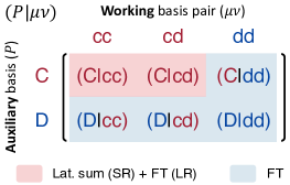
Figure 1: Schematic illustration of how different components of the three-center integrals [Eq. 6] are evaluated in RSGDF. Both the auxiliary and the AO bases are split into a compact (“C/c”) set and diffuse (“D/d”) set. The compact integrals (shaded in red) are range separated to yield short-range (SR) and long-range (LR) contributions that are evaluated in real space (by lattice summation) and in reciprocal space (by Fourier transforms), respectively; the diffuse integrals (shaded in blue) are evaluated entirely in reciprocal space using Fourier transforms. Note that the column corresponding to “dc”-type pair densities is similar to the “cd”-column and hence omitted for simplicity.

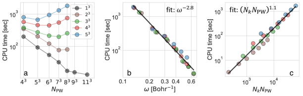
Figure 2: Timing of RSGDF for diamond/cc-pVDZ using $N_{k}=1^{3}$ to $5^{3}$. (a) Total DF initialization CPU time as a function of the number of PWs used to compute the LR integrals [Eqs. 15 and 10]. (b) CPU time for computing the SR integrals [Eq. 12] as a function of $\omega$ for all $k$-point meshes except for $N_{k}=1^{3}$. (c) CPU time for computing the LR integrals [Eqs. 15 and 10] as a function of $N_{k}N_{\mathrm{PW}}$ for all $k$-point meshes except for $N_{k}=1^{3}$. For (b) and (c), the black lines are power law fits to all data points leading to exponents as shown.

Since $N_{\mathrm{cell}}^{\mathrm{AFT}}$ and $N_{\mathrm{cell}}$ can be as large as $10^{4}$, the phase factor contractions in both Eqs. 11 and 12 would account for most of the computational cost (except for very small $k$-point meshes). However, if the $k$-points are sampled from a uniform (e.g. Monkhorst-Pack Monkhorst and Pack (1976)) mesh that includes the $\Gamma$ point, then the phase factors satisfy $\mathrm{e}^{\mathrm{i}\bm{k}\cdot\bm{m}}=\mathrm{e}^{\mathrm{i}\bm{k}\cdot(\bm{\tilde{m}}+\bm{M})}=\mathrm{e}^{\mathrm{i}\bm{k}\cdot\bm{\tilde{m}}}$, where $\bm{\tilde{m}}$ is inside the Born-von Karman supercell and $\bm{M}$ is a lattice translation vector of the Born-von Karman supercell. For example, the summation in Eq. 12 can then be rewritten as

$$\sum_{\bm{\tilde{m}}\bm{\tilde{n}}}^{N_{k}}\mathrm{e}^{-\mathrm{i}\bm{k}_{1}\cdot\bm{\tilde{m}}}\mathrm{e}^{\mathrm{i}\bm{k}_{2}\cdot\bm{\tilde{n}}}\sum_{\bm{m}\to\bm{\tilde{m}},\bm{n}\to\bm{\tilde{n}}}(V_{P\mu\nu}^{\bm{0},\bm{m}\bm{n}})^{\mathrm{SR}}_{\omega},$$ (14)

where the phase factor contraction now costs $O(N_{k}^{3}n_{\mathrm{aux}}n_{\mathrm{AO}}^{2})$; a similar treatment for Eq. 11 gives $O(N_{k}^{3}N_{\mathrm{PW}}n_{\mathrm{AO}}^{2})$ cost for the phase factor contraction. This process significantly reduces the total cost of these contractions so that they are subdominant (at least for moderately sized $k$-point meshes where $N_{k}$ is much smaller than $N_{\mathrm{cell}}$ or $N_{\mathrm{cell}}^{\mathrm{AFT}}$). The remaining cost-determining steps are the real-space integral evaluations in Eqs. 11 and 13a, which as a reminder scale as $O(N_{k}N_{\mathrm{cell}}^{\mathrm{AFT}}N_{\mathrm{PW}}n_{\mathrm{AO}}^{2})$ and $O(N_{\mathrm{cell}}n_{\mathrm{aux}}n_{\mathrm{AO}}^{2})$, respectively. Note that the cost of these expensive steps is no worse than linear in the number of auxiliary Gaussian basis functions.

The algorithm described so far yields significant performance improvements over existing periodic GDF schemes. We have identified an additional minor improvement, motivated by the observation that the real-space lattice summations needed for the SR part are slow to converge because of diffuse orbitals, i.e. those with small Gaussian exponents (recall that the FFT can be used in the LR part for diffuse orbitals). Therefore, we split both the auxiliary and the AO bases into a compact (“C/c”, upper case for auxiliary) and a diffuse (“D/d”) set based on a cutoff $\alpha^{\mathrm{cut}}$ for the primitive Gaussian exponents. Similar ideas of compact and diffuse basis splitting have also been explored by Pulay and co-workers for molecular calculations. Füsti-Molnar and Pulay (2002b) This leads us to six types of three-center integrals as shown in Fig. 1. Four of the integral types have either a diffuse bra or a diffuse ket (shaded in blue; note that both “cc” and “cd” are compact) and can thus be readily evaluated in reciprocal space using a relatively small PW basis Füsti-Molnar and Pulay (2002b) without range separation,

$$V_{P\mu\nu}^{\bm{k}_{1}\bm{k}_{2}}=4\pi\sum_{\bm{G}}^{N_{\mathrm{PW}}}{}^{{}^{\prime}}\frac{\tilde{\chi}_{P}^{\bm{k}_{12}}(-\bm{G})\tilde{\rho}_{\mu\nu}^{\bm{k}_{1}\bm{k}_{2}}(\bm{G})}{|\bm{G}+\bm{k}_{12}|^{2}}.$$ (15)

To summarize, in RSGDF, we evaluate these four integral types directly in reciprocal space and the remaining two integral types with compact bra and ket using the range separation scheme defined above. Note that the expensive AFTs of the compact auxiliary orbitals and pair densities can be calculated once and used in the evaluation of both integral types. In practice, a large majority of orbitals are defined as compact and so we find that this separation of orbitals speeds up our calculations by a factor of two or less compared to a direct application of RSGDF for all orbitals.

While the above presentation suggests a computational scaling that is linear in $N_{k}$ for typical mesh densities, the actual scaling is complicated by the choice of the parameters, $N_{\mathrm{PW}}$, $\omega$, and $\alpha^{\mathrm{cut}}$, which we discuss more below. Empirically we find that the optimal choice of $N_{\mathrm{PW}}$ scales as $O(N_{k}^{-1/2})$ (Fig. S3), and the overall cost of RSGDF scales roughly as $O(N_{k}^{0.8})$ for all the systems tested in this work (Fig. S6). However, this sublinear scaling only holds for small $N_{k}$, because $N_{\mathrm{PW}}$ eventually reaches a minimum value. Beyond that point, the AFTs needed for the LR part dominate the cost and we expect a linear scaling of RSGDF with $N_{k}$, at least for medium-sized $k$-point meshes.

Computational details. We implemented RSGDF as presented above in a local version of the PySCF software package Sun et al. (2018). We test its performance in terms of precision, accuracy, and computational efficiency using three simple three-dimensional solids: diamond, MgO, and LiF. For diamond, we perform all-electron calculations using the cc-pVDZ basis Dunning (1989); for MgO and LiF, we use GTH pseudopotentials Goedecker, Teter, and Hutter (1996); Hartwigsen, Goedecker, and Hutter (1998) and the corresponding GTH-DZVP basis VandeVondele et al. (2005). We use the cc-pVDZ-jkfit basis Weigend (2002) and the even-tempered basis (ETB) generated with a progression factor $\beta=2.0$ for the auxiliary expansion of the cc-pVDZ and the GTH-DZVP bases, respectively.

We compare RSGDF to GDF Sun et al. (2017), GPW (called FFTDF in PySCF) VandeVondele et al. (2005), and RSJK Sun (2020), as implemented in PySCF. For RSJK, we use eq. (23) in ref. Sun, 2020 to determine an appropriate $\omega$ for a given system and $k$-point mesh. For RSGDF, we manually test a range of $N_{\mathrm{PW}}$ and for each we determine the maximum $\omega$ and $\alpha^{\mathrm{cut}}$ that guarantee precision $\epsilon$ in all integrals; future work will focus on the automated selection of these parameters. As a general trend, using a larger PW basis slows down the LR part by increasing the number of expensive real-space integrations to be performed in Eq. 11 but accelerates the SR part by allowing larger values for $\omega$ and $\alpha^{\mathrm{cut}}$; a smaller PW basis has the opposite effect. Unless otherwise mentioned, all calculations are run with a target precision of $\epsilon=10^{-8}$ a.u. for integral evaluation, which is the default setting for production-level periodic calculations in PySCF. The finite-size error of the HF exchange energy is corrected with a Madelung constant, which yields $O(N_{k}^{-1})$ convergence to the thermodynamic limit Paier et al. (2006); Broqvist, Alkauskas, and Pasquarello (2009); Sundararaman and Arias (2013) (see Sec. S3 for details); other possibilities exist Gygi and Baldereschi (1986); Spencer and Alavi (2008); Guidon, Hutter, and VandeVondele (2009); Sundararaman and Arias (2013) but would require modification of the DF algorithm. All timing data reported below are the CPU time recorded using a single CPU core (Intel Xeon Gold 6126 2.6 GHz) with $16$ GB of memory and $100$ GB of disk space except for GPW which requires larger memory for $N_{k}\geq 4^{3}$. The current implementations of GDF and RSGDF are not integral-direct, meaning that we solve Eq. 4 only once and save the coefficients $\{\mathbf{d}^{\bm{k}_{1}\bm{k}_{2}}\}$ to disk for later use; this step is called “DF initialization” below and requires $O(N_{k}^{2}n_{\mathrm{aux}}n_{\mathrm{AO}}^{2})$ disk space which limits our calculations to a maximum $k$-point mesh of $N_{k}=5^{3}$ for all three systems. The other two methods, GPW and RSJK, are both implemented in an integral-direct manner and hence require little disk space. An integral-direct implementation of RSGDF tailored for specific applications will be presented in future work.

Results and discussion. We first verify our scaling analysis of the CPU cost of RSGDF. In Fig. 2a, we show the RSGDF initialization time as a function of $N_{\mathrm{PW}}$ for diamond using $N_{k}=1^{3}$ to $5^{3}$ $k$-points (recall that all calculations achieve the same target precision). The optimal $N_{\mathrm{PW}}$ – identified as the minimum on each curve – indeed decreases with $N_{k}$ as $O(N_{k}^{-1/2})$ (the fitted exponent is about $-0.44$; see Fig. S3). The inverse cubic dependence of the SR time on $\omega$ is verified in Fig. 2b, and the linear scaling of the LR time with $N_{k}N_{\mathrm{PW}}$ is verified in Fig. 2c. Similar results are observed for the other two systems (Figs. S1 and S2), although the optimal values of $N_{\mathrm{PW}}$ for a given $N_{k}$ vary slightly from system to system. We leave the automatic determination of the optimal $N_{\mathrm{PW}}$ to a future work as it requires a more careful calibration. In what follows, we will simply use the manually optimized values from Fig. 2a and Figs. S1a and S2a (summarized in Tab. S1).

The different choices of $N_{\mathrm{PW}}$ (and hence $\omega$ and $\alpha^{\mathrm{cut}}$) in RSGDF do not cause any inconsistency in the computed energies. As shown in Fig. S4, the converged RSGDF HF energies differ from the GDF results by less than $10^{-7}~{}E_{\mathrm{h}}$ for diamond and MgO and about $10^{-6}~{}E_{\mathrm{h}}$ for LiF for all data points shown in Fig. 2 and Figs. S1 and S2. We attribute the larger deviation observed for LiF to the linear dependency found in the auxiliary basis. Nonetheless, these deviations are acceptable as they are at least one order of magnitude smaller than the error introduced by DF itself (vide infra). Beyond the HF energy, we have also verified that the electron correlation energy of diamond computed with RSGDF using the second order Møller-Plesset perturbation theory Møller and Plesset (1934) agrees with the GDF results to better than $10^{-8}~{}E_{\mathrm{h}}$ for all $k$-point meshes tested (Tab. S2). These observations confirm that the algorithmic developments in RSGDF cause negligible precision loss compared to the original implementation of GDF.

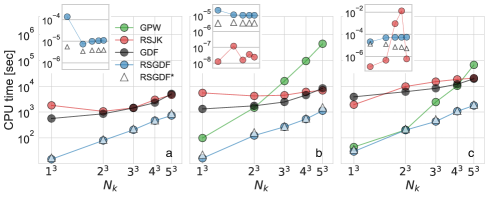
Figure 3: CPU time (per SCF cycle) for computing the Coulomb and the exchange integrals in a HF calculation for (a) diamond/cc-pVDZ, (b) MgO/GTH-DZVP, and (c) LiF/GTH-DZVP using GPW (green), RSJK (red), GDF (grey), and RSGDF (blue) to handle the ERIs. For GDF and RSGDF, the DF initialization time is included. For RSGDF, results using a larger auxiliary basis are also included (RSGDF*, white triangles). Precise timing data are given in Table S3. Insets show the deviation of the RSGDF HF energies from RSJK for diamond (a) and deviations of the RSGDF and the RSJK HF energies from GPW for MgO (b) and LiF (c), where the x-axis is $N_{k}$ and the y-axis is in $E_{\mathrm{h}}$.

Next, we study the computational efficiency of RSGDF. In Fig. 3, we plot the per-SCF-cycle time as a function of $N_{k}$ for computing the Coulomb and the exchange integrals in a HF calculation for all three systems using four different methods to handle the ERIs: GPW (green), RSJK (red), GDF (grey), and RSGDF (blue). Since the first two are implemented in an integral-direct fashion, we include the DF initialization time for GDF and RSGDF to enable a fair comparison.

We first compare GDF and RSGDF, which both compute the three-center integrals through a SR part in real space and a LR part in reciprocal space. Although both methods exhibit a similar sublinear scaling with $N_{k}$ at large $N_{k}$, only the GDF timings plateau at small $N_{k}$. This difference arises from the adjustment of the PW basis size for each $N_{k}$ and for each system (Tab. S1), which ultimately balances the SR-LR cost in RSGDF as analyzed above (Fig. S5). More importantly, the algorithmic optimizations developed for RSGDF in this work significantly reduce its computational cost and lead to speedups of one to two orders of magnitude over the previous GDF for all three systems studied here.

We next compare RSGDF with the two other methods without DF error, i.e. GPW and RSJK. The GPW timing shows the characteristic $O(N_{k}^{2})$ scaling of computing exact exchange starting from $N_{k}=2^{3}$ and is 40 to 400 times slower than RSGDF for the largest $N_{k}$ tested here. The very high cost of GPW for MgO is caused by the compact primitive Gaussians in the $2s$ and $2p$ orbitals of Mg, which require $83^{3}$ PWs to reach the target precision of $10^{-8}$ (cf. $51^{3}$ for LiF). We emphasize that lowering the precision requirement for GPW (hence lowering $N_{\mathrm{PW}}$) only moderately reduces the cost due to the $O(N_{\mathrm{PW}}\ln N_{\mathrm{PW}})$ scaling of FFT. For example, using $\epsilon=10^{-6}$ and $10^{-4}$ requires $75^{3}$ and $66^{3}$ PWs for MgO and reduces the cost by only factors of $1.4$ and $2.1$, respectively.

The RSJK timings are similar to those of GPW; although they show a slightly weaker dependence on $N_{k}$, the precise scaling is unclear. This peculiar $N_{k}$-dependence of RSJK arises from a significant SR-LR cost unbalance (Fig. S5) and suggests a breakdown of eq. (23) in ref. Sun, 2020 for determining the optimal $\omega$ for RSJK. Despite this, RSJK still achieves computational efficiency similar to GDF and much higher than GPW for moderately sized $k$-point meshes, which is remarkable given that RSJK does not use DF.

Finally, we examine the accuracy of the HF energies computed by RSGDF, which is a combination of the DF error due to the auxiliary basis set and the precision error when calculating the matrices in Eqs. 5 and 6. The RSJK results are used as the benchmark for diamond and the GPW results are used as the benchmark for MgO and LiF. To probe the possibility of achieving higher accuracy with DF, we also include results for RSGDF using a larger auxiliary basis (denoted by “RSGDF*” in Fig. 3); we use the cc-pVTZ-jkfit basis for diamond and an ETB whose size is about 1.25 times larger (obtained by using a smaller $\beta$) for MgO and LiF. The per-atom errors of the converged HF energies are plotted in the insets of Fig. 3.

With the default auxiliary basis, the error introduced by RSGDF is about $10^{-5}~{}E_{\mathrm{h}}$ for diamond and MgO and about $10^{-4}~{}E_{\mathrm{h}}$ for LiF; these errors are typical for DF-based HF calculations Burow, Sierka, and Mohamed (2009); Patterson (2020). Using the slightly larger auxiliary basis (RSGDF*) reduces the error by a factor of three or more and, most remarkably, requires little extra work as can be seen from the nearly identical timings of RSGDF and RSGDF* in Fig. 3. This is because the LR part is dominated by the AFTs of the orbital pair densities, Eq. 11, whose cost is independent of $n_{\mathrm{aux}}$, while the SR part scales linearly with $n_{\mathrm{aux}}$. By contrast, the accuracy of RSJK is in general very high ($10^{-7}~{}E_{\mathrm{h}}$ or less), but relatively large errors of about $10^{-2}~{}E_{\mathrm{h}}$ are also observed for certain $k$-point meshes (inset of Fig. 3c); the accuracy loss in the latter cases is likely due to an inaccurate integral screening, as tightening the precision to $10^{-10}$ reduces the error to about $10^{-5}~{}E_{h}$ for the calculation of LiF using $4^{3}$ $k$-points. These results demonstrate that RSGDF provides an extremely cost-effective approach to calculating accurate HF energies in periodic systems.

Conclusion. To summarize, we have presented an efficient scheme that uses range separation for Gaussian density fitting (RSGDF) for periodic systems. The computational scaling is analyzed to be sublinear with $N_{k}$ for small $k$-point meshes and linear for medium-sized ones. With all-electron and pseudopotential-based numerical results on a few three-dimensional solids, we verified the scaling of RSGDF and showed that it achieves about $10$-fold speedups over the previously developed GDF with little precision loss. The error introduced by RSGDF is about $10^{-5}~{}E_{\mathrm{h}}$ with default auxiliary basis sets and can be systematically reduced by increasing the size of the auxiliary basis with little extra work.

The primary purpose of the current integral-indirect implementation of RSGDF is to speed up Hartree-Fock (and hybrid density functional theory) calculations for a given Gaussian basis and auxiliary basis. Motivated by the excellent performance seen in these preliminary calculations, we are currently working on the automatic determination of the optimal $N_{\mathrm{PW}}$, $\omega$, and $\alpha^{\mathrm{cut}}$. Looking forward, the fast integral construction enabled by RSGDF encourages the development of integral-direct algorithms tailored to specific tasks such as the evaluation of exact exchange Wang, Lewis, and Valeev (2020), the ERI orbital transformation Maschio et al. (2007); Usvyat et al. (2007), and post-HF calculations Usvyat et al. (2007); Luenser, Schurkus, and Ochsenfeld (2017). Such integral-direct methods would significantly reduce the high memory footprint currently required by post-HF calculations on periodic systems with Gaussian basis sets.

Supplementary material

See the supplementary material for (i) RSGDF initialization time for different choices of $N_{\mathrm{PW}}$ and $\omega$ for MgO and LiF; (ii) optimal choices of $N_{\mathrm{PW}}$ for $N_{k}$ from $1^{3}$ to $5^{3}$ and different systems; (iii) difference of the HF energies computed using RSGDF and GDF; (iv) SR and LR component time of RSGDF, GDF, and RSJK for varying size of $k$-point meshes; (v) $N_{k}$-scaling of RSGDF and GDF for the timing data shown in Fig. 3; (vi) values of the parameters needed by RSGDF, GDF, RSJK, and GPW; (vii) comparison of the MP2 correlation energies computed using RSGDF and GDF for diamond; (viii) CPU time for computing the Coulomb and exchange integrals per SCF cycle by RSGDF, GDF, RSJK, and GPW; (ix) Details of the treatment of exchange divergence; (x) derivations of the conditions for prescreening the double lattice summation in Eq. 12.

Data availability statement

The data that support the findings of this study are available from the corresponding author upon reasonable request.

References

- Dovesi et al. (2018) R. Dovesi, A. Erba, R. Orlando, C. M. Zicovich-Wilson, B. Civalleri, L. Maschio, M. Rérat, S. Casassa, J. Baima, S. Salustro, and B. Kirtman, Wiley Interdiscip. Rev. Comput. Mol. Sci 8, e1360 (2018).
- Sun et al. (2018) Q. Sun, T. C. Berkelbach, N. S. Blunt, G. H. Booth, S. Guo, Z. Li, J. Liu, J. D. McClain, E. R. Sayfutyarova, S. Sharma, S. Wouters, and G. K.-L. Chan, Wiley Interdiscip. Rev. Comput. Mol. Sci 8, e1340 (2018).
- Kühne et al. (2020) T. D. Kühne, M. Iannuzzi, M. Del Ben, V. V. Rybkin, P. Seewald, F. Stein, T. Laino, R. Z. Khaliullin, O. Schütt, F. Schiffmann, D. Golze, J. Wilhelm, S. Chulkov, M. H. Bani-Hashemian, V. Weber, U. Borštnik, M. Taillefumier, A. S. Jakobovits, A. Lazzaro, H. Pabst, T. Müller, R. Schade, M. Guidon, S. Andermatt, N. Holmberg, G. K. Schenter, A. Hehn, A. Bussy, F. Belleflamme, G. Tabacchi, A. Glö, M. Lass, I. Bethune, C. J. Mundy, C. Plessl, M. Watkins, J. VandeVondele, M. Krack, and J. Hutter, J. Chem. Phys. 152, 194103 (2020).
- Balasubramani et al. (2020) S. G. Balasubramani, G. P. Chen, S. Coriani, M. Diedenhofen, M. S. Frank, Y. J. Franzke, F. Furche, R. Grotjahn, M. E. Harding, C. Hättig, A. Hellweg, B. Helmich-Paris, C. Holzer, U. Huniar, M. Kaupp, A. Marefat Khah, S. Karbalaei Khani, T. Müller, F. Mack, B. D. Nguyen, S. M. Parker, E. Perlt, D. Rappoport, K. Reiter, S. Roy, M. Rückert, G. Schmitz, M. Sierka, E. Tapavicza, D. P. Tew, C. van Wüllen, V. K. Voora, F. Weigend, A. Wodyński, and J. M. Yu, J. Chem. Phys. 152, 184107 (2020).
- Ihm, Zunger, and Cohen (1979) J. Ihm, A. Zunger, and M. L. Cohen, J. Phys. C: Solid State Phys. 12, 4409 (1979).
- Car and Parrinello (1985) R. Car and M. Parrinello, Phys. Rev. Lett. 55, 2471 (1985).
- Martins and Cohen (1988) J. L. Martins and M. L. Cohen, Phys. Rev. B 37, 6134 (1988).
- Pickett (1989) W. E. Pickett, Comput. Phys. Rep. 9, 115 (1989).
- Kresse and Furthmüller (1996) G. Kresse and J. Furthmüller, Comput. Mater. Sci. 6, 15 (1996).
- Maschio and Usvyat (2008) L. Maschio and D. Usvyat, Phys. Rev. B 78, 073102 (2008).
- Izmaylov and Scuseria (2008) A. F. Izmaylov and G. E. Scuseria, Phys. Chem. Chem. Phys. 10, 3421 (2008).
- Hirata and Shimazaki (2009) S. Hirata and T. Shimazaki, Phys. Rev. B 80, 085118 (2009).
- Maschio et al. (2010) L. Maschio, D. Usvyat, M. Schütz, and B. Civalleri, J. Chem. Phys. 132, 134706 (2010).
- McClain et al. (2017) J. McClain, Q. Sun, G. K.-L. Chan, and T. C. Berkelbach, J. Chem. Theory Comput. 13, 1209 (2017).
- Sun et al. (2017) Q. Sun, T. C. Berkelbach, J. D. McClain, and G. K.-L. Chan, J. Chem. Phys. 147, 164119 (2017).
- Wang and Berkelbach (2020) X. Wang and T. C. Berkelbach, J. Chem. Theory Comput. 16, 3095 (2020).
- Buchholz and Stein (2018) H. K. Buchholz and M. Stein, J. Comput. Chem. 39, 1335 (2018).
- VandeVondele et al. (2005) J. VandeVondele, M. Krack, F. Mohamed, M. Parrinello, T. Chassaing, and J. Hutter, Comput. Phys. Commun. 167, 103 (2005).
- Whitten (1973) J. L. Whitten, J. Chem. Phys. 58, 4496 (1973).
- Dunlap, Connolly, and Sabin (1979) B. I. Dunlap, J. W. D. Connolly, and J. R. Sabin, J. Chem. Phys. 71, 3396 (1979).
- Mintmire and Dunlap (1982) J. W. Mintmire and B. I. Dunlap, Phys. Rev. A 25, 88 (1982).
- Baerends, Ellis, and Ros (1973) E. Baerends, D. Ellis, and P. Ros, Chem. Phys. 2, 41 (1973).
- Vahtras, Almlöf, and Feyereisen (1993) O. Vahtras, J. Almlöf, and M. Feyereisen, Chem. Phys. Lett. 213, 514 (1993).
- Jung et al. (2005) Y. Jung, A. Sodt, P. M. W. Gill, and M. Head-Gordon, Proc. Natl. Acad. Sci. 102, 6692 (2005).
- Reine et al. (2008) S. Reine, E. Tellgren, A. Krapp, T. Kjærgaard, T. Helgaker, B. Jansik, S. Høst, and P. Salek, J. Chem. Phys. 129, 104101 (2008).
- Hill (2013) J. G. Hill, Int. J. Quantum Chem. 113, 21 (2013).
- Sodt, Subotnik, and Head-Gordon (2006) A. Sodt, J. E. Subotnik, and M. Head-Gordon, J. Chem. Phys. 125, 194109 (2006).
- Sodt and Head-Gordon (2008) A. Sodt and M. Head-Gordon, J. Chem. Phys. 128, 104106 (2008).
- Manzer et al. (2015) S. Manzer, P. R. Horn, N. Mardirossian, and M. Head-Gordon, J. Chem. Phys. 143, 024113 (2015).
- Werner, Manby, and Knowles (2003) H.-J. Werner, F. R. Manby, and P. J. Knowles, J. Chem. Phys. 118, 8149 (2003).
- Eshuis, Yarkony, and Furche (2010) H. Eshuis, J. Yarkony, and F. Furche, J. Chem. Phys. 132, 234114 (2010).
- Werner and Schütz (2011) H.-J. Werner and M. Schütz, J. Chem. Phys. 135, 144116 (2011).
- Riplinger and Neese (2013) C. Riplinger and F. Neese, J. Chem. Phys. 138, 034106 (2013).
- Györffy et al. (2013) W. Györffy, T. Shiozaki, G. Knizia, and H.-J. Werner, J. Chem. Phys. 138, 104104 (2013).
- Varga (2005) v. Varga, Phys. Rev. B 71, 073103 (2005).
- Varga, Milko, and Noga (2006) v. Varga, M. Milko, and J. Noga, J. Chem. Phys. 124, 034106 (2006).
- Maschio et al. (2007) L. Maschio, D. Usvyat, F. R. Manby, S. Casassa, C. Pisani, and M. Schütz, Phys. Rev. B 76, 075101 (2007).
- Usvyat et al. (2007) D. Usvyat, L. Maschio, F. R. Manby, S. Casassa, M. Schütz, and C. Pisani, Phys. Rev. B 76, 075102 (2007).
- Pisani et al. (2008) C. Pisani, L. Maschio, S. Casassa, M. Halo, M. Schütz, and D. Usvyat, J. Comput. Chem. 29, 2113 (2008).
- Burow, Sierka, and Mohamed (2009) A. M. Burow, M. Sierka, and F. Mohamed, J. Chem. Phys. 131, 214101 (2009).
- Lazarski, Burow, and Sierka (2015) R. Lazarski, A. M. Burow, and M. Sierka, J. Chem. Theory Comput. 11, 3029 (2015).
- Luenser, Schurkus, and Ochsenfeld (2017) A. Luenser, H. F. Schurkus, and C. Ochsenfeld, J. Chem. Theory Comput. 13, 1647 (2017).
- Grundei and Burow (2017) M. M. J. Grundei and A. M. Burow, J. Chem. Theory Comput. 13, 1159 (2017).
- Wang, Lewis, and Valeev (2020) X. Wang, C. A. Lewis, and E. F. Valeev, J. Chem. Phys. 153, 124116 (2020).
- Usvyat, Maschio, and Schütz (2017) D. Usvyat, L. Maschio, and M. Schütz, “Periodic local møller-plesset perturbation theory of second order for solids,” in Handbook of Solid State Chemistry (American Cancer Society, 2017) Chap. 3, pp. 59–86.
- Patterson (2020) C. H. Patterson, J. Chem. Phys. 153, 064107 (2020).
- Lazarski et al. (2016) R. Lazarski, A. M. Burow, L. Grajciar, and M. Sierka, J. Comput. Chem. 37, 2518 (2016).
- Becker and Sierka (2019) M. Becker and M. Sierka, J. Comput. Chem. 40, 2563 (2019).
- Varga (2008) v. Varga, Int. J. Quantum Chem. 108, 1518 (2008).
- Varga (2011) v. Varga, J. Math. Chem. 49, 1 (2011).
- Merlot et al. (2013) P. Merlot, T. Kjærgaard, T. Helgaker, R. Lindh, F. Aquilante, S. Reine, and T. B. Pedersen, J. Comput. Chem. 34, 1486 (2013).
- Schmitz and Christiansen (2018) G. Schmitz and O. Christiansen, Chem. Phys. Lett. 701, 7 (2018).
- Wirz, Reine, and Pedersen (2017) L. N. Wirz, S. S. Reine, and T. B. Pedersen, J. Chem. Theory Comput. 13, 4897 (2017).
- Shimazaki, Kosugi, and Nakajima (2014) T. Shimazaki, T. Kosugi, and T. Nakajima, J. Phys. Soc. Japan 83, 054702 (2014).
- Sharma and Beylkin (2020) S. Sharma and G. Beylkin, “Efficient evaluation of gaussian integrals in periodic systems,” (2020), arXiv:2010.05400 .
- Grüneis, Marsman, and Kresse (2010) A. Grüneis, M. Marsman, and G. Kresse, J. Chem. Phys. 133, 074107 (2010).
- Grüneis (2015) A. Grüneis, J. Chem. Phys. 143, 102817 (2015).
- Hummel, Gruber, and Grüneis (2016) F. Hummel, T. Gruber, and A. Grüneis, Eur. Phys. J. B 89, 235 (2016).
- Mayr-Schmölzer et al. (2020) W. Mayr-Schmölzer, J. Planer, J. Redinger, A. Grüneis, and F. Mittendorfer, Phys. Rev. Research 2, 043361 (2020).
- Pisani and Dovesi (1980) C. Pisani and R. Dovesi, Int. J. Quantum Chem. 17, 501 (1980).
- Dovesi et al. (2000) R. Dovesi, R. Orlando, C. Roetti, C. Pisani, and V. Saunders, phys. stat. sol. (b) 217, 63 (2000).
- Sun (2020) Q. Sun, “Exact exchange matrix of periodic hartree-fock theory for all-electron simulations,” (2020), arXiv:2012.07929 .
- Gill and Adamson (1996) P. M. Gill and R. D. Adamson, Chem. Phys. Lett. 261, 105 (1996).
- Füsti-Molnar and Pulay (2002a) L. Füsti-Molnar and P. Pulay, J. Chem. Phys. 116, 7795 (2002a).
- Füsti-Molnar and Pulay (2002b) L. Füsti-Molnar and P. Pulay, J. Chem. Phys. 117, 7827 (2002b).
- Monkhorst and Pack (1976) H. J. Monkhorst and J. D. Pack, Phys. Rev. B 13, 5188 (1976).
- Dunning (1989) T. H. Dunning, J. Chem. Phys. 90, 1007 (1989).
- Goedecker, Teter, and Hutter (1996) S. Goedecker, M. Teter, and J. Hutter, Phys. Rev. B 54, 1703 (1996).
- Hartwigsen, Goedecker, and Hutter (1998) C. Hartwigsen, S. Goedecker, and J. Hutter, Phys. Rev. B 58, 3641 (1998).
- Weigend (2002) F. Weigend, Phys. Chem. Chem. Phys. 4, 4285 (2002).
- Paier et al. (2006) J. Paier, M. Marsman, K. Hummer, G. Kresse, I. C. Gerber, and J. G. Ángyán, J. Chem. Phys. 124, 154709 (2006).
- Broqvist, Alkauskas, and Pasquarello (2009) P. Broqvist, A. Alkauskas, and A. Pasquarello, Phys. Rev. B 80, 085114 (2009).
- Sundararaman and Arias (2013) R. Sundararaman and T. A. Arias, Phys. Rev. B 87, 165122 (2013).
- Gygi and Baldereschi (1986) F. Gygi and A. Baldereschi, Phys. Rev. B 34, 4405 (1986).
- Spencer and Alavi (2008) J. Spencer and A. Alavi, Phys. Rev. B 77, 193110 (2008).
- Guidon, Hutter, and VandeVondele (2009) M. Guidon, J. Hutter, and J. VandeVondele, J. Chem. Theory Comput. 5, 3010 (2009).
- Møller and Plesset (1934) C. Møller and M. S. Plesset, Phys. Rev. 46, 618 (1934).