Learning Rate Optimization for Federated Learning Exploiting Over-the-air Computation

Abstract

Federated learning (FL) as a promising edge-learning framework can effectively address the latency and privacy issues by featuring distributed learning at the devices and model aggregation in the central server. In order to enable efficient wireless data aggregation, over-the-air computation (AirComp) has recently been proposed and attracted immediate attention. However, fading of wireless channels can produce aggregate distortions in an AirComp-based FL scheme. To combat this effect, the concept of dynamic learning rate (DLR) is proposed in this work. We begin our discussion by considering multiple-input-single-output (MISO) scenario, since the underlying optimization problem is convex and has closed-form solution. We then extend our studies to more general multiple-input-multiple-output (MIMO) case and an iterative method is derived. Extensive simulation results demonstrate the effectiveness of the proposed scheme in reducing the aggregate distortion and guaranteeing the testing accuracy using the MNIST and CIFAR10 datasets. In addition, we present the asymptotic analysis and give a near-optimal receive beamforming design solution in closed form, which is verified by numerical simulations.

I Introduction

Future sixth-generation (6G) communication networks are envisioned to undergo a profound transformation, which evolves from connected things to connected intelligence with more stringent requirements such as dense networking, strict security, high energy efficiency, and high intelligence [1, 2]. Artificial intelligence (AI) technologies, which allows automatic analysis of a large mass of data generated in wireless networks and subsequent optimization of highly dynamic and complex network [3, 4, 5], will shape the landscape of 6G. Conversely, 6G will give renewed impetus to the AI-empowered mobile applications by supplying the advanced wireless communications and mobile computing technologies [6] as supporting infrastructure.

AI tasks entail increasingly intensive computation workloads. Hence, they are generally migrated to and trained on the server center with sufficient computation resources and the availability of data that is first collected from the devices/sensors and then uploaded to the center [7, 8]. The data volume can be considerably large and, thus, imposing heavy transmission traffic burden and increasing the latency. Another critical problem comes from the serious concern of privacy leakage, since the generated data, e.g., photos, social-networking records, at the devices are often privacy sensitive. An intuitive way to counteract the above issues would be to conduct training and inference process directly at the network edge, such as devices and sensors, using locally generated real-time data. The paradigm edge learning has unique advantages of balanced resource support, proximity to data sources compared with cloud learning and higher learning accuracy compared to on-device learning by harnessing the computation and storage capacities [9, 10].

Federated learning (FL) tackles the aforementioned concerns by collaboratively training a shared global model with locally stored data [11, 12, 13, 14]. A typical FL algorithm alternates between two iterative phases: (I) The devices receive the global model from the edge server and train local models with locally stored data; (II) These local models are transmitted to and aggregated at the edge server to yield the global model. Note that the data volume of the local models (may consist of millions of parameters) are much smaller than the raw data. Nonetheless, the local models uploaded by legion of participating devices via wireless links is resource-demanding, which is the main bottleneck to implement FL in practice. In this regard, developing communication-efficient methods are of paramount importance. Some recent works have considered asynchronous mechanism [15], quantization [16, 17], sparsification [18, 19], and aggregate frequency [20] to reduce the transmission overhead, which, however, ignore the aspects of physical and network layers.

In the second phase of FL, the edge server averages the local model parameters from the distributed devices, which is essentially wireless data aggregation. Conventional multiple-access schemes, such as orthogonal frequency-division multiple access (OFDM), are based on the separated-communication-and-computing principle. In [21], a time-division multiple access (TDMA) system was considered, where a joint batchsize selection and communication resource allocation scheme was developed aiming at accelerating the training process and improving the learning efficiency. The impact of three different scheduling policies on the FL performance were analytically studied in the large-scale wireless networks [22]. Such sub-optimal communication-and-computation approaches could result in a sharp rise in consumption of wireless resources as well as congesting the air-interface [9]. Very Recently, the over-the-air computation (AirComp) scheme was proposed by leveraging the waveform superposition property of multiple-access channels, which is fundamentally different from the traditional separated-communication-and-computing principle [23]. By aggregating the data simultaneously received from distributed devices in an analog manner, the AirComp technique can further improve communication efficiency [24, 25, 26].

The AirComp technique has recently been applied to implementing FL. Specifically, a gradient sparsification and random linear projection based approach is proposed and the reduced data was transmitted via AirComp to address the bandwidth and power limitations, which outperformed its digital counterpart [24, 25]. As a matter of fact, the distortions caused by fading and noisy channels are critical for learning tasks as a large aggregation error may lead to the degradation of inference accuracy. In [26], the transmission power was designed by truncated channel inversion, and two scheduling schemes were proposed to guarantee the identical amplitudes of the received signals among devices in a single-input-single-output (SISO) system to reduce the aggregate error. Meanwhile in [27], joint device selection and receive beamforming design was investigated in single-input-multiple-output (SIMO) configuration, and a novel unified difference-of-convex (DC) function was proposed. On the other hand, the problem of distortion minimization in an intelligent reflection surface (IRS)-aided cloud radio access network (CRAN) system was addressed in [28], where a joint optimization scheme of the passive beamforming and linear detection vector was designed. Furthermore, with the aid of multi-IRS, a novel resource and device selection method was developed to minimize the aggregate error as well as maximize the selected devices [29]. The existing works utilized wireless resources, such as power control, device selection and beamforming design, as well as channel configuration to align the received signals from distributed devices. Nevertheless, they did not fully unleash the potential of hyper-parameters in the perspective of machine learning (ML).

Learning rate is a key hyper-parameter that determines the convergence and the convergence rate of the learning tasks. A large learning rate will hinder convergence and cause loss function around the minimum or even to diverge, while too small a learning rate will lead to slow convergence [30]. To select an optimal learning rate is always critical, yet tricky issue for learning algorithms to work properly. One feasible approach is to adopt learning rate schedulers, which is able to adjust the learning rate training online. However, it has to be designed in advance and is unable to adapt to the characteristics of the dataset [31]. Adaptive learning rates such as Adagrad can adapt to the data and change with the gradients, which are most widely used in deep learning community [32]. Later, cyclical learning rate (CLR) was proposed to allow the learning rate cyclically vary between reasonable boundary values, which incurs less computational cost and can significantly enhance the learning performance [33]. The essence behind CLR originates from the observation that increasing the learning rate allows more rapid traversal of saddle point plateaus and thus achieves a longer term beneficial effect. Inspired by this study, we propose dynamic learning rate (DLR) between the minimum and maximum boundaries to adapt to the fading channels, in order to further reduce the aggregate error caused by the fading and noisy channels.

In this paper, we consider FL for AI-empowered mobile applications, such as e-health services, which will be supported by 6G networks. Instead of adopting conventional separated-communication-and-computation pattern, we incorporate AirComp to aggregate local models from distributed devices so as to improve the communication efficiency. In AirComp-based schemes, minimizing the resultant aggregate distortion is of paramount importance as a large distortion can spawn performance degradation of AI tasks. To mitigate the wireless distortion measured by mean square error (MSE), we first propose to utilize a DLR scheme to adapt to the wireless channels, and receive beamforming optimization is jointly considered. The technical contributions of this work are summarized below.

• To our best knowledge, this is the first work to study the use of DLR for FL over wireless communications to reduce the aggregate error, which is fundamentally different from existing works which only consider the optimization of wireless resources. We analytically show that DLR can be properly designed to mitigate the distortion caused by fading. It is also proved that the MSE can be further decreased by considering DLR.

• For MSE minimization via AirComp, we jointly optimize the DLR ratios and wireless resources. Both MISO and MIMO scenarios are considered, and the respective closed-form solution and iterative algorithm are developed. Extensive simulation results demonstrate the effectiveness of the proposed scheme in further reducing the MSE as well as improving the learning performance on MNIST and CIFAR10 datasets.

• In addition, we present the asymptotic beamforming solution in closed form when the number of transmit/receive antennas tends to infinity. Simulation results verify the theoretical analysis as well as the receive beamforming design.

The outline of this paper is organized as follows: Some necessary mathematical descriptions of FL and AirComp are presented in Section II. The concept of DLR is introduced in Section III. In Section IV and Section V, the DLR optimization problems in MISO and MIMO scenarios are respectively formulated and solved. Next, we present the theoretical asymptotic analysis and, on this basis, propose a near-optimal and closed-form receive beamforming solution in Section VI. Then, in Section VII, numerical simulations are provided to showcase the advantages of the proposed scheme. Finally, the paper is concluded in Section VIII.

II Preliminary

In this work, we consider the problem of FL over wireless networks. The configuration of the system under investigation is depicted in Fig. 1. The wireless network consist of $K$ devices with $N_{d}$ antennas each and an aggregator with $N_{t}$ antennas. The set of devices are denoted as $\mathcal{K}$. Each device $k$ updates its model based on locally distributed data $\mathcal{D}_{k}$, which cannot be shared with other entities out of latency and privacy concerns.

Figure 1: An FL system over wireless communication.

II-A FL

FL has recently emerged as an effective distributed approach to enable wireless devices to collaboratively build a shared learning model with training taken place locally. The objective of FL is to minimize the aggregate loss:

$$\boldsymbol{w}^{o}\triangleq\underset{\boldsymbol{w}}{\mathrm{argmin}}\frac{1}{K}\sum\nolimits_{k=1}^{K}P_{k}\left(\boldsymbol{w}\right),$$ (1)

where $\boldsymbol{w}\in\mathbb{R}^{D}$ is a vector containing the model parameters, $D$ is the dimension of the FL model, $P_{k}\left(\boldsymbol{w}\right)$ is the local loss value at device $k$ based on $\mathcal{D}_{k}$, given by

$$P_{k}\left(\boldsymbol{w}\right)\triangleq\frac{1}{\left|\mathcal{D}_{k}\right|}\sum\nolimits_{n=1}^{\left|\mathcal{D}_{k}\right|}Q_{k}\left(\boldsymbol{w};\boldsymbol{x}_{n},y_{n}\right),$$ (2)

where $Q_{k}$ is the loss function on the sample $\left(\boldsymbol{x}_{n},y_{n}\right)$ with $\boldsymbol{x}_{n},y_{n}$ the input and the label. To obtain the solution of (1), a centralized gradient decent method is applied and the parameters are updated as

$$\boldsymbol{w}^{i+1}=\boldsymbol{w}^{i}-\mu\left(\frac{1}{K}\sum\nolimits_{k=1}^{K}\boldsymbol{g}_{k}\left(\boldsymbol{w}^{i}\right)\right),$$ (3)

where $i$ is the iteration index, $\mu$ is the learning rate, $\boldsymbol{g}_{k}(\boldsymbol{w}^{i})=\nabla_{\boldsymbol{w}}P_{k}\left(\boldsymbol{w}^{i}\right)$ is the gradient of loss with respect to $\boldsymbol{w}^{i}$. Hereinafter, we denote $\boldsymbol{g}_{k}(\boldsymbol{w}^{i})$ by $\boldsymbol{g}_{k}$ for notation simplicity. Since the aggregator is inaccessible to the data distributed at any particular device $k$, the gradient term $\boldsymbol{g}_{k}$ is calculated locally and the local model, denoted as $\boldsymbol{w}_{k}$, is updated accordingly. By introducing the local learning rate denoted as $\mu_{k}$, the local model at device $k$ is updated by

$$\boldsymbol{w}_{k}^{i+1}=\boldsymbol{w}^{i}-\mu_{k}\boldsymbol{g}_{k}.$$ (4)

With local models received at the aggregator, the update of the global model (3) is rewritten as

$$\boldsymbol{w}^{i+1}=\frac{1}{K}\sum\nolimits_{k=1}^{K}\boldsymbol{w}_{k}^{i+1}.$$ (5)

II-B AirComp

As introduced earlier, AirComp integrates computation and communication by exploiting the waveform superposition property, which harnesses interference to help functional computation [23]. The AirComp comprises three stages: (i) Pre-processing at the transmitters; (ii) Superposition over the air; and (iii) Post-processing at the receiver [34]. In this work, the pre-processing is assumed to be identity mapping. Each parameter in a local model is modulated as a symbol, then the symbol vector $\boldsymbol{s}_{k}^{i+1}\triangleq\boldsymbol{w}_{k}^{i+1}\in\mathbb{C}^{D}$ is obtained accordingly. The symbol vector is assumed to be normalized by the unit variance, which is given by $\mathbb{E}\left[\boldsymbol{s}_{k}^{i+1}\left(\boldsymbol{s}_{k}^{i+1}\right)^{\mathrm{H}}\right]=\mathbf{I}$. For notation simplicity, the $d$-th element of $\boldsymbol{s}_{k}$, $\boldsymbol{w}^{i}$ and $\boldsymbol{g}_{k}$, i.e., $\boldsymbol{s}_{k}[d]$, $\boldsymbol{w}^{i}\left[d\right]$ and $\boldsymbol{g}_{k}[d]$, are written as $s_{k}$, $w^{i}$ and $g_{k}$. As such, the desired signal based on (3) can be represented by

$$y_{\mathrm{des}}\!=\!\frac{1}{K}\!\sum\nolimits_{k=1}^{K}\!s_{k}\!=\!\frac{1}{K}\!\sum\nolimits_{k=1}^{K}\!w_{k}^{i+1}\!=\!w^{i}\!-\frac{\mu}{K}\sum\nolimits_{k=1}^{K}\!g_{k}.$$ (6)

Considering the multiple access channel property of wireless communication, the received signal is a linear sum of the transmitted signal plus uncertainty. Hence, after the post-processing, the received signal at the receiver can be expressed as

$$y=\sqrt{\eta}\left(\sum\nolimits_{k=1}^{K}A_{k}s_{k}+B\right),$$ (7)

where $s_{k}$ is the input of the communication system from device $k$, and $\eta$ is a scaling factor. The variables $A_{k}$ and $B$ depend on the specific scenario settings. In particular, we have $A_{k}=h_{k}b_{k}$ and $B=n$ for SISO; $A_{k}=\boldsymbol{h}_{k}^{\mathrm{T}}\boldsymbol{b}_{k}$ and $B=n$ for MISO. For SIMO and MIMO scenarios, we have $A_{k}=\boldsymbol{m}^{\mathrm{H}}\boldsymbol{h}_{k}b_{k}$, $B=\boldsymbol{m}^{\mathrm{H}}\boldsymbol{n}$, and $A_{k}=\boldsymbol{m}^{\mathrm{H}}\boldsymbol{H}_{k}\boldsymbol{b}_{k}$, $B=\boldsymbol{m}^{\mathrm{H}}\boldsymbol{n}$, respectively. Note that $h_{k}\left(\boldsymbol{h}_{k},\boldsymbol{H}_{k}\right)$ is the independent Rayleigh fading channel (vector/matrix) from device $k$ to the aggregator, which is assumed to be block fading and remain constant during the process of model transmission; $b_{k}\left(\boldsymbol{b}_{k}\right)$ is the transmit coefficient (vector) at device $k$; $\boldsymbol{m}$ is the receive beamforming vector at the aggregator; $n\left(\boldsymbol{n}\right)$ is the noise (vector) with power of $\sigma^{2}$.

Instead of obtaining the individual term $s_{k}$ first and then averaging at the aggregator, we employ AirComp to estimate the desired signal directly. The AirComp aggregate error is defined as the difference between the desired signal and its estimation, which is derived as

$$\begin{array}[]{*{20}{l}}e\triangleq\displaystyle y_{\mathrm{des}}-y=\frac{1}{K}\sum\nolimits_{k=1}^{K}s_{k}-\sqrt{\eta}\left(\sum\nolimits_{k=1}^{K}A_{k}s_{k}+B\right)\\ \;\;\,\displaystyle=\sum\nolimits_{k=1}^{K}\left(\frac{1}{K}-\sqrt{\eta}A_{k}\right)s_{k}-\sqrt{\eta}B.\end{array}$$ (8)

According to (8), the aggregate distortion originates from both fading and noise, which are reflected in the fading-channel-related term $\sqrt{\eta}A_{k}$ and the noise-related term $\sqrt{\eta}B$, respectively. It is worth noting that mitigating the distortion is of great importance, as severe distortion can result in a biased global model and, in turn, degrades the learning performance.

III DLR for Channel Adaption

Existing works [28, 27, 29, 26] minimize the aggregate error by means of wireless resource optimization, IRS-based channel reconfiguration, and device selection. These approaches correspond to optimize the transmit coefficient (vector) $b_{k}\left(\boldsymbol{b}_{k}\right)$, the receive beamforming vector $\boldsymbol{m}$, the scaling factor $\eta$, and the passive beamforming vector $\Theta$, or simply select a subset of the devices. Though appears different at first glance, these approaches share a common aim, which is to align the receive signals and minimize the noise-induced error. Whereas in this work, we take a radically different perspective and propose to mitigate the distortions by optimizing the hyper-parameters in the learning process. Concretely, a strategy is designed to let the local learning rate $\mu_{k}$ adapt to the time-varying wireless environment. Based on the aforementioned features of FL and AirComp, we arrive at the following theorem.

Theorem 1.

Denote DLR ratio as $r_{k}=\frac{\mu_{k}}{\mu}$ for device $k$, to mitigate the distortion caused by the fading channel related term $\sqrt{\eta}A_{k}$, we have

$$\sqrt{\eta}\sum\nolimits_{k=1}^{K}A_{k}=1,\quad r_{k}=\frac{1}{K\sqrt{\eta}A_{k}}.$$ (9)

Proof.

The aggregate error $e^{ch}$ caused by the fading channels can be written as

$$e^{ch} =y_{\mathrm{des}}-\sqrt{\eta}\sum\nolimits_{k=1}^{K}A_{k}s_{k}$$

$$=\left(w^{i}\!-\!\frac{\mu}{K}\sum\nolimits_{k=1}^{K}g_{k}\right)\!-\!\sqrt{\eta}\sum\nolimits_{k=1}^{K}A_{k}\left(w^{i}\!-\!\mu_{k}g_{k}\right)$$

$$=\left(1\!-\!\sqrt{\eta}\sum_{k=1}^{K}A_{k}\right)w^{i}\!+\!\sum_{k=1}^{K}\left(\sqrt{\eta}A_{k}\mu_{k}\!-\!\frac{\mu}{K}\right)g_{k},$$ (10)

which is mitigated if and only if both terms $\left(\frac{1}{K}\mu-\sqrt{\eta}A_{k}\mu_{k}\right)$ and $\left(1-\sqrt{\eta}\sum_{k=1}^{K}A_{k}\right)$ are $0$. Thus, we directly obtain (9). ∎

Based on Theorem 1, the residual aggregate error is the noise-related term $\sqrt{\eta}B$, which can be measured by

$$\mathrm{MSE}=\eta\mathbb{E}\left(\left\|B\right\|^{2}\right).$$ (11)

For simplicity, we consider the retransmission mechanism such that if there exists aggregate error, the probability of retransmission is

$$P=1-\exp\left(-\frac{a\mathrm{\left\|\mathit{e}\right\|^{2}}}{p_{\mathrm{des}}}\right),$$ (12)

where $a$ is the modulation-related parameter [35], $p_{\mathrm{des}}$ denotes the power of the desired signal, and $e$ is the aggregate error. Intuitively, a larger aggregate error leads to a larger retransmission rate.

IV Problem Formulation

The objective is to minimize the MSE metric given in (11), subject to equality constraint (9) and boundary constraint $r_{k}=\mu_{k}/\mu\in\left[r_{\min},r_{\max}\right]$. In this section, we establish the problem formulations for both MISO and MIMO cases, which will be shown in the sequel are respectively convex and nonconvex. It is important to note that SISO and SIMO can be regarded as the special cases of MISO and MIMO scenarios, respectively.

IV-A MISO

In the MISO scenario, the devices equipped with $N_{d}$ antennas each transmit their models to the single-antenna aggregator. Under this scenario, we have $A_{k}=\boldsymbol{h}_{k}^{\mathrm{T}}\boldsymbol{b}_{k}$ and $B=n$. The aggregate error measured by MSE is then given by

$$\mathrm{MSE}=\eta\mathbb{E}\left(\left\|B\right\|^{2}\right)=\eta\mathbb{E}\left(\left\|n\right\|^{2}\right)=\eta\sigma^{2}.$$ (13)

Since the noise power $\sigma^{2}$ is independent from the optimized variables, the problem can be formulated as

$$\min_{\eta,b_{k},r_{k}}\quad \eta$$

$$\mathrm{s.t.}\quad \sqrt{\eta}\sum\nolimits_{k=1}^{K}\boldsymbol{h}_{k}\boldsymbol{b}_{k}=1,$$ (14a)

$$r_{k}=\frac{1}{K\sqrt{\eta}\boldsymbol{h}_{k}\boldsymbol{b}_{k}},\quad\forall k,$$ (14b)

$$r_{k}\in\left[r_{\min},r_{\max}\right],\quad\forall k,$$ (14c)

$$\left\|\boldsymbol{b}_{k}\right\|^{2}\leq P_{k},\quad\forall k,$$ (14d)

where $P_{k}$ is the maximum transmit power at device $k$, and $\boldsymbol{h}_{k}\in\mathbb{C}^{N_{d}}$ is the channel vector between device $k$ and the aggregator. Both equality constraints (14a) and (14b) conspire to guarantee the elimination of error $e^{\mathrm{ch}}$ caused by the wireless fading channels as per Theorem 1.

Motivated by the uniform-forcing transceiver design in [36], the optimal transmitting coefficient vector $\boldsymbol{b}_{k}$ is designed as

$$\boldsymbol{b}_{k}=\frac{\boldsymbol{h}_{k}^{\mathrm{H}}}{K\sqrt{\eta}\left\|\boldsymbol{h}_{k}\right\|^{2}r_{k}}.$$ (15)

Power constraint (14d) further suggests that $\frac{1}{K^{2}P_{k}r_{k}^{2}\left\|\boldsymbol{h}_{k}\right\|^{2}}\leq\eta$, and thus we have

$$\eta=\max_{k}\frac{1}{K^{2}P_{k}r_{k}^{2}\left\|\boldsymbol{h}_{k}\right\|^{2}}.$$ (16)

We learn from (14b) that $\boldsymbol{h}_{k}^{\mathrm{T}}\boldsymbol{b}_{k}=\frac{1}{K\sqrt{\eta}r_{k}}$. By substituting it back to (14a), we have $\sum_{k=1}^{K}\frac{1}{Kr_{k}}=1$. As a result, problem (14) is equivalent to

$$\underset{r_{k}}{\min}\quad \max_{k}\frac{1}{K^{2}P_{k}r_{k}^{2}\left\|\boldsymbol{h}_{k}\right\|^{2}}$$ (17a)

$$\mathrm{s.t.}\quad \sum\nolimits_{k=1}^{K}\frac{1}{Kr_{k}}=1,$$ (17b)

$$r_{k}\in\left[r_{\min},r_{\max}\right],\quad\forall k.$$ (17c)

Remark 1.

As a special case of the MISO scenario where $A_{k}=h_{k}b_{k}$ and $B=n$, the problem formulated under the SISO case is similar to (17). The only difference lies in the channel and transmit coefficients, which are both complex scalars instead of vectors in the MISO case.

IV-B MIMO

In the MIMO scenario, each device and the aggregator are equipped with $N_{d}$ and $N_{t}$ antennas, respectively. The terms $A_{k}$ and $B$ in (7) are $A_{k}=\boldsymbol{m}^{\mathrm{H}}\boldsymbol{H}_{k}\boldsymbol{b}_{k}$, $B=\boldsymbol{m}^{\mathrm{H}}\boldsymbol{n}$ with $\boldsymbol{m}$ the receive beamforming vector. Accordingly, the aggregate error measured by MSE is expressed as

$$\mathrm{MSE}\!=\!\eta\mathbb{E}\left(\!\left\|B\right\|^{2}\!\right)\!=\!\eta\mathbb{E}\left(\!\left\|\boldsymbol{m}^{\mathrm{H}}\boldsymbol{n}\right\|^{2}\!\right)\!=\!\sigma^{2}\!\left\|\boldsymbol{m}\right\|^{2}\!\eta,$$ (18)

where $\boldsymbol{n}$ the independent Gaussian noise vector. Based on Theorem 1, the MSE minimization problem can be formulated as

$$\min_{\boldsymbol{m},\eta,r_{k},\boldsymbol{b}_{k}}\quad \left\|\boldsymbol{m}\right\|^{2}\eta$$ (19a)

$$\mathrm{s.t.\quad} \sqrt{\eta}\sum\nolimits_{k=1}^{K}\boldsymbol{m}^{\mathrm{H}}\boldsymbol{H}_{k}\boldsymbol{b}_{k}=1,$$ (19b)

$$r_{k}=\frac{1}{K\sqrt{\eta}\boldsymbol{m}^{\mathrm{H}}\boldsymbol{H}_{k}\boldsymbol{b}_{k}},\quad\forall k,$$ (19c)

$$r_{k}\in\left[r_{\min},r_{\max}\right],\quad\forall k,$$ (19d)

$$\left\|\boldsymbol{b}_{k}\right\|^{2}\leq P_{k},\quad\forall k,$$ (19e)

where $\boldsymbol{b}_{k}\in\mathbb{C}^{N_{d}},\boldsymbol{H}_{k}\in\mathbb{C}^{N_{t}\times N_{d}},\boldsymbol{m\in\mathbb{C}}^{Nt}$ are the transmitting beamforming vector at device $k$, the channel matrix between the aggregator and device $k$, and the receive beamforming vector at the aggregator, respectively. According to the constraints (19c), the optimal transmitting coefficient can be readily obtained [36], i.e.,

$$\boldsymbol{b}_{k}=\frac{\boldsymbol{H}_{k}^{\mathrm{H}}\boldsymbol{m}}{K\sqrt{\eta}r_{k}\left\|\boldsymbol{m}^{\mathrm{H}}\boldsymbol{H}_{k}\right\|^{2}}.$$ (20)

Power constraint (19e) further indicates that $\eta\geq\frac{1}{K^{2}P_{k}r_{k}^{2}\left\|\boldsymbol{m}^{\mathrm{H}}\boldsymbol{H}_{k}\right\|^{2}}$ for each device $k$, which implies

$$\eta=\underset{k}{\max}\frac{1}{K^{2}P_{k}r_{k}^{2}\left\|\boldsymbol{m}^{\mathrm{H}}\boldsymbol{H}_{k}\right\|^{2}}.$$ (21)

Similar to the MISO scenario, the ratio $r_{k}$ satisfies $\sum_{k=1}^{K}\frac{1}{Kr_{k}}=1$, which can be easily derived from the equality constraints (14a) and (14b). Problem (19) can then be rewritten as

$$\min_{\boldsymbol{m},r_{k}}\quad \underset{k}{\max}\frac{\left\|\boldsymbol{m}\right\|^{2}}{K^{2}P_{k}r_{k}^{2}\left\|\boldsymbol{m}^{\mathrm{H}}\boldsymbol{H}_{k}\right\|^{2}}$$ (22a)

$$\mathrm{s.t.\quad} \sum_{k=1}^{K}\frac{1}{Kr_{k}}=1,$$ (22b)

$$r_{k}\in\left[r_{\min},r_{\max}\right],\quad\forall k.$$ (22c)

Proposition 1.

Problem (22) is equivalent to

$$\min_{\boldsymbol{m},r_{k}}\quad \underset{k}{\max}\frac{\left\|\boldsymbol{m}\right\|^{2}}{K^{2}P_{k}r_{k}^{2}\left\|\boldsymbol{m}^{\mathrm{H}}\boldsymbol{H}_{k}\right\|^{2}}$$ (23a)

$$(\ref{eq:pro1-2-1-1}),\,(\ref{eq:pro1_3-1-1}),$$

$$\left\|\boldsymbol{m}\right\|=1.$$ (23b)

Proof.

$\forall\boldsymbol{m}$ can be written as the multiplication of its norm and the unit direction vector, i.e., $\boldsymbol{m}=\left\|\boldsymbol{m}\right\|\frac{\boldsymbol{m}}{\left\|\boldsymbol{m}\right\|}.$ If we let $\tilde{\boldsymbol{m}}=\frac{\boldsymbol{m}}{\parallel\boldsymbol{m}\parallel}$, the objective function of problem (22) is equivalent to $\underset{k}{\max}\frac{\left\|\tilde{\boldsymbol{m}}\right\|^{2}}{K^{2}P_{k}r_{k}^{2}\left\|\tilde{\boldsymbol{m}}^{\mathrm{H}}\boldsymbol{H}_{k}\right\|^{2}},$ where $\left\|\tilde{\boldsymbol{m}}\right\|=1$. This completes the proof. ∎

Remark 2.

The SIMO scenario is a special case of the MIMO case, where $A_{k}=\boldsymbol{m}^{\mathrm{H}}\boldsymbol{h}_{k}b_{k}$, $B=\boldsymbol{m}^{\mathrm{H}}\boldsymbol{n}$. The problem formulated under SIMO case is the same as (23) except that the channel and transmit coefficients are respectively vector $\boldsymbol{h}_{k}\in\mathbb{C}^{N_{t}}$ and scalar $b_{k}\in\mathbb{C}$.

V DLR Optimization

In this section, we develop two algorithms to solve problems (17) and (23), respectively. For the MISO scenario, problem (17) is convex and a closed-form solution is derived. For nonconvex problem (23), we decompose the problem into two sub-problems and propose an iterative method by alternately fixing one variable and solving for the other.

V-A MISO

Obviously, problem (17) is convex. For notation simplicity, we let $l_{k}=\frac{1}{r_{k}}$ and $c_{k}=\frac{1}{K\sqrt{P_{k}}\left\|\boldsymbol{h}_{k}\right\|}$. As such, problem (17) can be written as

$$\underset{l_{k}}{\min}\quad \max_{k}\left(c_{k}l_{k}\right)^{2}$$ (24a)

$$\mathrm{s.t.}\quad \sum\nolimits_{k=1}^{K}l_{k}=K,$$ (24b)

$$\frac{1}{r_{\max}}\leq l_{k}\leq\frac{1}{r_{\min}},\quad\forall k.$$ (24c)

The solution that minimizes $\max_{k}\left(c_{k}l_{k}\right)^{2}$ also minimizes $\max_{k}c_{k}l_{k}$, which indicates that their solutions are identical. Consequently, problem (24) is further equivalent to the following problem

$$\underset{l_{k}}{\min}\,\max_{k}c_{k}l_{k}\quad\mathrm{s.t.}\>(\ref{eq:SIMO_C1}),\,(\ref{eq:SIMO_C2}),$$ (25)

which is a typical linear programming problem.

Assuming $k=\mathrm{arg}\max_{i}c_{i}l_{i}$, we then have $c_{i}l_{i}\leq c_{k}l_{k}$ for all $i$. Following the equation constraint (24b), we have

$$K=\sum\nolimits_{i=1}^{K}l_{i}\leq\sum\nolimits_{i=1}^{K}\frac{c_{k}l_{k}}{c_{i}}=c_{k}l_{k}\sum\nolimits_{i=1}^{K}\frac{1}{c_{i}}.$$ (26)

Thus

$$c_{k}l_{k}\geq\frac{K}{\sum_{i=1}^{K}\frac{1}{c_{i}}}.$$ (27)

Theorem 2.

In a MISO system, the MSE is lower bounded by $\mathrm{MSE^{lb}}=\frac{\sigma^{2}}{\left(\sum_{i=1}^{K}\sqrt{P_{i}}\left\|\boldsymbol{h}_{i}\right\|\right)^{2}}$. Denoting the MSE obtained with and without considering DLR as $\mathrm{MSE^{d}}$ and $\mathrm{MSE^{n}}$, we always have

$$\mathrm{MSE^{n}}\overset{\left(a\right)}{\geq}\mathrm{MSE^{d}}\overset{\left(b\right)}{\geq}\mathrm{MSE^{lb}},$$ (28)

where equality $\left(a\right)$ holds if and only if $\sqrt{P_{i}}\left\|\boldsymbol{h}_{i}\right\|=\sqrt{P_{j}}\left\|\boldsymbol{h}_{j}\right\|,\forall i,j\in\mathcal{K}$, and equality $\left(b\right)$ holds if and only if $r_{i}\sqrt{P_{i}}\left\|\boldsymbol{h}_{i}\right\|=r_{j}\sqrt{P_{j}}\left\|\boldsymbol{h}_{j}\right\|,\forall i,j\in\mathcal{K}$.

Proof.

According to (27), the lower bound of $c_{k}l_{k}$ is $\frac{K}{\sum_{i=1}^{K}\frac{1}{c_{i}}}$. Hence, the MSE is lower bounded by

$$\mathrm{MSE^{lb}}=\left(\frac{K}{\sum_{i=1}^{K}\frac{1}{c_{i}}}\right)^{2}\sigma^{2}=\frac{\sigma^{2}}{\left(\sum_{i=1}^{K}\sqrt{P_{i}}\left\|\boldsymbol{h}_{i}\right\|\right)^{2}}.$$ (29)

The lower bound is attained if and only if $c_{i}l_{i}=c_{j}l_{j},\forall i,j\in\mathcal{K}$, which also means that $r_{i}\sqrt{P_{i}}\left\|\boldsymbol{h}_{i}\right\|=r_{j}\sqrt{P_{j}}\left\|\boldsymbol{h}_{j}\right\|,\forall i,j\in\mathcal{K}$.

With loss of generality, we assume that $c_{k}$ is sorted in a descending order, i.e., $c_{i}\geq c_{j},\forall i>j$. Thus, the MSE without considering DLR can be readily obtained as

$$\mathrm{MSE^{n}}=c_{1}^{2}\sigma^{2}=\frac{\sigma^{2}}{K^{2}P_{1}\left\|\boldsymbol{h}_{1}\right\|^{2}},$$ (30)

where $l_{k}$ can be regarded to have equal value of $1$. When taking the DLR into consideration, we can always find a feasible set of coefficients $\left[l_{1},l_{2},\ldots,l_{K}\right]$, which guarantee both $c_{1}\geq c_{1}l_{1}$ and $c_{1}l_{1}=\max\left(c_{i}l_{i},\forall i\in\mathcal{K}\right).$ Consequently, we have

$$\mathrm{MSE^{d}}=c_{1}^{2}l_{1}^{2}\sigma^{2}\leq c_{1}^{2}\sigma^{2}=\mathrm{MSE^{n}},$$ (31)

the equality of which holds if and only if when $c_{i}=c_{j},\forall i,j\in\mathcal{K}$, i.e., $\sqrt{P_{i}}\left\|\boldsymbol{h}_{i}\right\|=\sqrt{P_{j}}\left\|\boldsymbol{h}_{j}\right\|,\forall i,j\in\mathcal{K}$. Finally, we complete the proof. ∎

To further minimize the MSE, we should optimize $l_{i}$. Based on the above analysis, the optimal solution of $l_{i}$ under constraint (24c) is given by

$$l_{i}=\mathrm{clip}\left(\frac{c_{k}l_{k}}{c_{i}},\left[\frac{1}{r_{\max}},\frac{1}{r_{\min}}\right]\right),$$ (32)

where

$$\sum_{i=1}^{K}l_{i}=K.$$ (33)

Operation $\mathrm{clip}\left(x,\left[a,b\right]\right)$ truncates $x$ to the specified interval $\left[a,b\right]$.

The overall procedure to solve problem (24) is shown in Algorithm 1. According to (32), the proposed scheme needs to know the user index $k$ with the maximum value $c_{k}l_{k}$. To find the device index, we exhaustively search all devices, which indicates that the number of iterations in the outer layer is $K$. For a given device index $k$, the bisection technique is applied to find a solution $l_{k}$, the complexity of which is $\mathcal{O}(\log_{2}(1/\delta))$ with accuracy $\delta$.

Algorithm 1 Optimal Learning Rate for MISO.

Input: $c_{k}$, ${\mathrm{obj}}=\frac{\max_{k}(c_{k})}{r_{\min}}$, $\delta$, $\mathrm{Num}=20$
Output: $l_{i}^{\mathrm{opt}},{\mathrm{obj}}$
Initialize: $l_{k}^{\mathrm{min}}=\frac{1}{r_{\max}}$, $l_{k}^{\mathrm{max}}=\frac{1}{r_{\min}}$

1:for $k=1:K$

2: while $|\sum_{i=1}^{K}l_{i}-K|\leq\delta$

3:  $l_{k}=(l_{k}^{\mathrm{max}}+l_{k}^{\mathrm{min}})/2$

4:  $l_{i}=\mathrm{clip}\left(\frac{c_{k}l_{k}}{c_{i}},[\frac{1}{r_{\max}},\frac{1}{r_{\min}}]\right),\forall i\in\mathcal{K}$

5:  if ($\sum_{i=1}^{K}l_{i}\geq K$)

6:   $l_{k}^{\mathrm{max}}=l_{k}$

7:  else

8:   $l_{k}^{\mathrm{min}}=l_{k}$

9: if ${\mathrm{obj}}\geq\max(c_{i}l_{i})$

10:  ${\mathrm{obj}}=\max(c_{i}l_{i})$

11:  $l_{i}^{\mathrm{opt}}=l_{i},\forall i\in\mathcal{K}$

V-B MIMO

Suppose that $c_{k}=\frac{\left\|\boldsymbol{m}\right\|}{K\sqrt{P_{k}}\left\|\boldsymbol{m}^{\mathrm{H}}\boldsymbol{H}_{k}\right\|}$, $l_{k}=\frac{1}{r_{k}}$, and $c_{k}l_{k}=\max_{i}\left(c_{i}l_{i}\right)$, we have the following theorem.

Theorem 3.

In a MIMO system, the MSE is lower bounded by $\mathrm{MSE^{lbm}}=\frac{\sigma^{2}}{\left(\sum_{i=1}^{K}\sqrt{P_{i}}\left\|\boldsymbol{m}^{\mathrm{H}}\boldsymbol{H}_{i}\right\|\right)^{2}}$ for any given $\boldsymbol{m}$, and we always have

$$\mathrm{MSE^{n}}\overset{\left(a\right)}{\geq}\mathrm{MSE^{d}}\overset{\left(b\right)}{\geq}\mathrm{MSE^{lbm}},$$ (34)

where the equalities of $\left(a\right)$ and $\left(b\right)$ hold when $\sqrt{P_{i}}\left\|\boldsymbol{m}^{\mathrm{H}}\boldsymbol{H}_{i}\right\|=\sqrt{P_{j}}\left\|\boldsymbol{m}^{\mathrm{H}}\boldsymbol{H}_{j}\right\|,\forall i,j\in\mathcal{K}$, and $r_{i}\sqrt{P_{i}}\left\|\boldsymbol{m}^{\mathrm{H}}\boldsymbol{H}_{i}\right\|=r_{j}\sqrt{P_{j}}\left\|\boldsymbol{m}^{\mathrm{H}}\boldsymbol{H}_{j}\right\|,\forall i,j\in\mathcal{K}$, respectively.

Proof.

According to the equality constraints (22b) and (23b), we arrive at

$$c_{k}l_{k}\!\geq\!\frac{K}{\sum\limits_{i=1}^{K}\displaystyle\frac{1}{c_{i}}}\!=\!\frac{\left\|\boldsymbol{m}\right\|}{\sum\limits_{i=1}^{K}\!\sqrt{P_{i}}\left\|\boldsymbol{m}^{\mathrm{H}}\boldsymbol{H}_{i}\right\|}\!=\!\frac{1}{\sum\limits_{i=1}^{K}\!\sqrt{P_{i}}\left\|\boldsymbol{m}^{\mathrm{H}}\boldsymbol{H}_{i}\right\|}.$$ (35)

Thus, $\mathrm{MSE^{lbm}}=\frac{\sigma^{2}}{\left(\sum_{i=1}^{K}\sqrt{P_{i}}\left\|\boldsymbol{m}^{\mathrm{H}}\boldsymbol{H}_{i}\right\|\right)^{2}}$ is the lower bound of MSE for any given feasible $\boldsymbol{m}$, which is achieved only if $c_{i}l_{i}=c_{j}l_{j},\forall i,j\in\mathcal{K}$, i.e., $r_{i}\sqrt{P_{i}}\left\|\boldsymbol{m}^{\mathrm{H}}\boldsymbol{H}_{i}\right\|=r_{j}\sqrt{P_{j}}\left\|\boldsymbol{m}^{\mathrm{H}}\boldsymbol{H}_{j}\right\|,\forall i,j\in\mathcal{K}$.

We first put aside the DLR and denote the equivalent channel as $\boldsymbol{h}^{\prime}_{i}=\boldsymbol{m}^{\mathrm{H}}\sqrt{P_{i}}\boldsymbol{H}_{i}\in\mathbb{C}^{N_{d}}$. As such, the problem of MSE minimization becomes to find $\boldsymbol{m}$ that maximizes the minimum $\ell_{2}$-norm of $\boldsymbol{h}^{\prime}_{i}$. Denoting its optimal solution as $\boldsymbol{m}^{*}$, the corresponding minimum $\ell_{2}$-norm and MSE can be expressed as $h_{\mathrm{min}}^{\mathrm{norm}}=\min\left(\sqrt{P_{i}}\left\|\boldsymbol{\left(m^{*}\right)}^{\mathrm{H}}\boldsymbol{H}_{i}\right\|\right)$, and $\mathrm{MSE}^{\mathrm{n}}=\frac{\sigma^{2}}{\left(Kh_{\mathrm{min}}^{\mathrm{norm}}\right)^{2}}$. Then, we consider the DLR in the following two cases.

Case 1: The lower bound is not attained, i.e., $\mathrm{MSE}^{\mathrm{n}}>\mathrm{MSE}^{\mathrm{lbm}}$. Without loss of generality, assume that $c_{k}$ is sorted in an ascending order, i.e., $\left\|\boldsymbol{h}_{i}^{\prime}\right\|\geq\left\|\boldsymbol{h}_{j}^{\prime}\right\|,\forall i>j$. There always exists a feasible set of DLR coefficients $\left[r_{1},r_{2},\ldots,r_{K}\right]$ such that $r_{K}\left\|\boldsymbol{h}_{K}^{\prime}\right\|>\left\|\boldsymbol{h}_{K}^{\prime}\right\|$ with $r_{K}\left\|\boldsymbol{h}_{K}^{\prime}\right\|=\min\left(r_{i}\left\|\boldsymbol{h}_{i}^{\prime}\right\|\right)$. Thus, $\mathrm{MSE}^{\mathrm{n}}>\mathrm{MSE}^{\mathrm{d}}\overset{\left(b\right)}{\geq}\mathrm{MSE^{lbm}}$, and the equality of $\left(b\right)$ holds only when $r_{i}\left\|\boldsymbol{h}_{i}^{\prime}\right\|=r_{j}\left\|\boldsymbol{h}_{j}^{\prime}\right\|,\forall i,j\in\mathcal{K}$.

Case 2: The lower bound is achieved i.e., $\mathrm{MSE}^{\mathrm{n}}=\mathrm{MSE}^{\mathrm{lbm}}$. In this case, we have $\left\|\boldsymbol{h}_{i}\right\|=\left\|\boldsymbol{h}_{j}\right\|,\forall i,j\in\mathcal{K}$ and $\mathrm{MSE}^{\mathrm{n}}=\mathrm{MSE}^{\mathrm{d}}=\mathrm{MSE}^{\mathrm{lbm}}$. The introduction of DLR cannot further improve the performance, and DLR in this case is equal to $1$.

Therefore, we complete the proof. ∎

In the MIMO scenario, problem (23) is difficult due to the nonconvex objective (23a) and constraint (23b). By introducing an auxiliary variable $\tau$, problem (23) is further equivalent to the following problem:

$$\min_{\boldsymbol{m},r_{k},\tau}\quad \tau$$ (36a)

$$\mathrm{s.t.\quad} \left\|\boldsymbol{m}\right\|^{2}\leq\tau K^{2}P_{k}\left\|\boldsymbol{m}^{\mathrm{H}}\boldsymbol{H}_{k}\right\|^{2}r_{k}^{2},\quad\forall k,$$ (36b)

$$(\ref{eq:pro1-2-1-1}),(\ref{eq:pro1_3-1-1}),(\ref{eq:SIMO2-2}).$$

To solve problem (36), we utilize the iterative technique and decompose the problem into two sub-problems by alternately fixing the DLR ratio $r_{k}$ and the receive beamforming vector $\boldsymbol{m}$, respectively.

Given the DLR ratio $r_{k}$, the original problem (36) is reduced into the following sub-problem:

$$\min_{\boldsymbol{m},\tau}\;\tau\qquad\mathrm{s.t.}\quad(\ref{eq:SIMO2-2}),(\ref{eq:SIMO3-2}),$$ (37)

which is nonconvex due to constraints (23b) and (36b). To solve problem (37), we have the following lemma.

Lemma 1.

Suppose that we have a semidefinite matrix $\boldsymbol{A}_{k}=\boldsymbol{H}_{k}\boldsymbol{H}_{k}^{\mathrm{H}}$, if $\det\boldsymbol{A}_{k}>0$, the range of $\frac{\left\|\boldsymbol{m}\right\|^{2}}{K^{2}P_{k}\left\|\boldsymbol{m}^{\mathrm{H}}\boldsymbol{H}_{k}\right\|^{2}r_{k}^{2}}$ is $\left[\frac{1}{K^{2}P_{k}r_{k}^{2}\lambda_{\mathrm{max}}},\frac{1}{K^{2}P_{k}r_{k}^{2}\lambda_{k,\mathrm{min}}}\right]$; otherwise $\left[\frac{1}{K^{2}P_{k}r_{k}^{2}\lambda_{k,\mathrm{max}}},\infty\right]$, where $\lambda_{k,\mathrm{max}}$ and $\lambda_{k,\mathrm{min}}$ are the maximum and minimum eigenvalues of $\boldsymbol{A}_{k}$, respectively.

Proof.

Define a function $g\left(\boldsymbol{m}\right)=\frac{\parallel\boldsymbol{m}^{\mathrm{H}}\boldsymbol{H}\parallel^{2}}{\parallel\boldsymbol{m}\parallel^{2}}=\frac{\boldsymbol{m}^{\mathrm{H}}\boldsymbol{H}\boldsymbol{H}^{\mathrm{H}}\boldsymbol{m}}{\boldsymbol{m}^{\mathrm{H}}\boldsymbol{m}},$ which is the Rayleigh-Ritz of matrix $\boldsymbol{A}=\boldsymbol{H}\boldsymbol{H}^{\mathrm{H}}$. Suppose that the maximum and minimum eigenvalues of $\boldsymbol{A}$ are respectively $\lambda_{\mathrm{max}}$ and $\lambda_{\mathrm{min}}$, function $g\left(\boldsymbol{m}\right)$ is within the interval of $\left[\lambda_{\mathrm{min}},\lambda_{\mathrm{max}}\right]$. Apparently, $\boldsymbol{A}\left(\neq\boldsymbol{0}\right)$ is semidefinite and we have $\det\boldsymbol{A}\geq 0$. In the case of $\det\boldsymbol{A}>0$, the eigenvalues of $\boldsymbol{A}$ are positive. Consequently, we have

$$\frac{1}{\lambda_{\mathrm{max}}}\leq\frac{1}{g\left(\boldsymbol{m}\right)}=\frac{\parallel\boldsymbol{m}\parallel^{2}}{\parallel\boldsymbol{m}^{\mathrm{H}}\boldsymbol{H}\parallel^{2}}\leq\frac{1}{\lambda_{\mathrm{min}}}.$$ (38)

Otherwise, $\lambda_{\mathrm{min}}=0$, we have

$$\frac{1}{\lambda_{\mathrm{max}}}\leq\frac{1}{g\left(\boldsymbol{m}\right)}=\frac{\parallel\boldsymbol{m}\parallel^{2}}{\parallel\boldsymbol{m}^{\mathrm{H}}\boldsymbol{H}\parallel^{2}}\leq\infty.$$ (39)

Therefore, the proof is complete. ∎

Remark 3.

Let $\tau_{k}^{l\mathrm{ow}}=\frac{1}{K^{2}P_{k}r_{k}^{2}\lambda_{k,\mathrm{max}}},$ $\tau_{k}^{\mathrm{up}}=\frac{1}{K^{2}P_{k}r_{k}^{2}\lambda_{k,\mathrm{min}}}$ if $\lambda_{\mathrm{min}}>0$; otherwise $\tau_{k}^{\mathrm{up}}=\infty$, and then $\frac{\left\|\boldsymbol{m}\right\|^{2}}{K^{2}P_{k}\left\|\boldsymbol{m}^{\mathrm{H}}\boldsymbol{H}_{k}\right\|^{2}r_{k}^{2}}\in\left[\tau_{k}^{\mathrm{low}},\tau_{k}^{\mathrm{up}}\right]$. The necessary condition of $\tau$ that guarantees the feasibility of problem (37) is $\text{$\tau\in$}\left[\tau^{\mathrm{low}},\tau^{\mathrm{up}}\right]$, where

$$\tau^{\mathrm{low}}=\min_{k}\left(\tau_{k}^{\mathrm{low}}\right),\>\tau^{\mathrm{up}}=\max_{k}\left(\tau_{k}^{\mathrm{up}}\right).$$ (40)

For any given $\tau\in\left[\tau^{\mathrm{low}},\tau^{\mathrm{up}}\right]$, sub-problem (37) is interpreted as finding the receive beamforming vector $\boldsymbol{m}$ that makes the sub-problem feasible, which is a check problem. By introducing $\boldsymbol{M}=\boldsymbol{m}\boldsymbol{m}^{\mathrm{H}}$, the sub-problem given $\tau$ is converted to

$$\min_{\boldsymbol{M}}\quad 0$$ (41a)

$$\mathrm{s.t.\quad} \mathrm{Tr}\left(\boldsymbol{M}\right)\leq\tau K^{2}P_{k}\mathrm{Tr}\left(\boldsymbol{M}\boldsymbol{H}_{k}\boldsymbol{H}_{k}^{\mathrm{H}}\right)r_{k}^{2},\quad\forall k,$$ (41b)

$$\boldsymbol{M}\succcurlyeq 0$$ (41c)

$$\mathrm{Tr}\left(\boldsymbol{M}\right)=1$$ (41d)

$$\mathrm{rank}\left(\boldsymbol{M}\right)=1.$$ (41e)

Indeed, the only difficulty of the above problem lies in the rank one constraint (41e). The problem can be solved by first dropping the constraint (41e) to obtain solution $\boldsymbol{M}^{*}$. Then, the receive beamforming vector $\boldsymbol{m}^{*}$ can be calculated using the eigenvector approximation method or the randomization technique [37], which is sub-optimal especially when $\boldsymbol{M}$ is large. To guarantee the rank one constraint, we utilize a DC representation [27, 38], and convert problem (41) to

$$\min_{\boldsymbol{M}}\;\mathrm{Tr}\left(\boldsymbol{M}\right)-\left\|\boldsymbol{M}\right\|_{2}\quad\mathrm{s.t.}\;(\ref{eq:pro3A1-1}),(\ref{eq:pro3A2-1}),(\ref{eq:pro3A3-1}),(\ref{eq:pro3A4-1}),$$ (42)

which can be efficiently solved by DC programming with complexity of $\mathcal{O}\left(N_{t}^{3}\right)$.

To find the solution $\tau$, we utilize the bisection technique. Specifically, the interval $\left[\tau^{\mathrm{low}},\tau^{\mathrm{up}}\right]$ is divided into two sub-intervals $\left[\tau^{\mathrm{low}},\tau\right]$ and $\left[\tau,\tau^{\mathrm{up}}\right]$ with $\tau=\left(\tau^{\mathrm{low}}+\tau^{\mathrm{up}}\right)/2.$ If problem (42) is solved for $\tau$, then the solution is within $\left[\tau^{\mathrm{low}},\tau\right]$; otherwise we have $\left[\tau,\tau^{\mathrm{up}}\right]$. Repeatedly checking the problem until $\tau^{\mathrm{up}}-\tau^{\mathrm{low}}<\delta$, where $\delta$ is the accuracy. Such bisection technique involves $\log_{2}\frac{1}{\delta}$ repetitive operations and, hence, solving the problem (37) requires the computational complexity of $\mathcal{O}\left(N_{t}^{3}\log_{2}\frac{1}{\delta}\right)$. The algorithm is summarized in Algorithm 2.

Algorithm 2 Beamforming design for MIMO.

Input: $\boldsymbol{H}^{\mathrm{H}}_{k}$, $r_{k}$, $\delta$
Output: $\boldsymbol{m}$, $\tau$

1:calculate $\tau^{\mathrm{low}}$, $\tau^{\mathrm{up}}$ based on (40)

2:while $(\tau^{\mathrm{up}}-\tau^{\mathrm{low}})>\delta$

3: if problem (42) is infeasible

4:  $\tau^{\mathrm{up}}=(\tau^{\mathrm{up}}+\tau^{\mathrm{low}})/2$

5: else

6:  $\tau^{\mathrm{low}}=(\tau^{\mathrm{up}}+\tau^{\mathrm{low}})/2$

Given the obtained receive beamforming vector $\boldsymbol{m}$, the original problem (36) is reduced to the sub-problem below:

$$\min_{r_{k},\tau}\quad\tau\qquad\mathrm{s.t.}\quad(\ref{eq:pro1-2-1-1}),(\ref{eq:pro1_3-1-1}),(\ref{eq:SIMO3-2}).$$ (43)

Denoting the equivalent channel vector $\boldsymbol{h}^{\prime}_{k}$ as $\boldsymbol{m}^{\mathrm{H}}\boldsymbol{H}_{k}$, the sub-problem (43) can be transformed into the problem under the MISO case with channel vector $\boldsymbol{h}^{\prime}_{k}$. Note that the sub-problem under the SIMO case is equivalent to that of the SISO case by defining equivalent channel coefficient $h^{\prime}_{k}$ as $\boldsymbol{m}^{\mathrm{H}}\boldsymbol{h}_{k}$. Therefore, we can readily derive the closed-form solution in the MISO case. We let $l_{k}=\frac{1}{r_{k}}$, $c_{k}=\frac{1}{K\sqrt{P_{k}}\left\|\boldsymbol{h}_{k}^{{}^{\prime}}\right\|}=\frac{1}{K\sqrt{P_{k}}\left\|\boldsymbol{m}^{\mathrm{H}}\boldsymbol{H}_{k}\right\|}$, and then the solution is given by $l_{i}=\mathrm{clip}\left(\frac{c_{k}l_{k}}{c_{i}},[\frac{1}{r_{\max}},\frac{1}{r_{\min}}]\right)$, where $\sum_{i=1}^{K}l_{i}=K$.

Thus, the sub-optimal solution of problem (36) can be obtained by alternatively solving sub-problems (42) and (43). For each iteration, the computational complexity is $\mathcal{O}\left(N_{t}^{3}\log_{2}\frac{1}{\delta_{1}}+K\log_{2}\frac{1}{\delta_{2}}\right)$, where $\delta_{1}$ and $\delta_{2}$ are the accuracy of solving receive beamforming vector $\boldsymbol{m}$ and DLR ratio $r_{k}$, respectively. The iterative method proposed is summarized in Algorithm 3.

Algorithm 3 Iterative Learning Rate and Receive Beamforming.

Input: $\boldsymbol{H}_{k}$
Output: $\boldsymbol{m}$, $r_{k}$, $\tau$
Initialize: $r_{k}=1$

1:do loop

2: given $r_{k}$, solve problem (37) using Algorithm 2

3: given $\boldsymbol{m}$, solve problem (43) using Algorithm 1

4:until $\tau$ converges

VI Asymptotic Analysis and Receive Beamforming Design

This section presents the theoretical analysis of the MSE and the DLR ratio in the MISO, SIMO, and MIMO scenarios, when the numbers of antennas $N_{d}$ and $N_{t}$ increase to infinity. Based on the asymptotic analysis, we propose a near-optimal and closed-form receive beamforming solution. Note that each device is assumed to have equal maximum power $P_{k}=P$.

VI-A MISO

In the MISO case, we present asymptotic analysis when the number of antennas $N_{d}$ at the devices goes to infinity. Since the channels between the devices and the aggregator are assumed to be independently Rayleigh distributed, we have

$$\left\|\boldsymbol{h}_{k}\right\|\rightarrow\sqrt{N_{d}},$$ (44)

$$c_{k}=\frac{1}{K\sqrt{P}\left\|\boldsymbol{h}_{k}\right\|}\rightarrow\frac{1}{K\sqrt{P}\sqrt{N_{d}}},$$ (45)

which suggest that $c_{i}=c_{j},\forall i,j\in\mathcal{K}$. As a consequence, lower bound $\mathrm{MSE^{lb}}$ can be achieved according to Theorem 2 and the equalities in both (a) and (b) of (28) are guaranteed. Accordingly, the MSE and $r_{k}$ become

$$\mathrm{MSE}=\left(\frac{1}{\sqrt{P}\sum_{i=1}^{K}\left\|\boldsymbol{h}_{i}\right\|}\right)^{2}\sigma^{2}\rightarrow\frac{\sigma^{2}}{PK^{2}N_{d}},$$ (46)

$$r_{k}=\frac{1}{l_{k}}=c_{k}\sqrt{P}\sum\nolimits_{i=1}^{K}\left\|\boldsymbol{h}_{i}\right\|=\frac{\sum_{i=1}^{K}\left\|\boldsymbol{h}_{i}\right\|}{K\left\|\boldsymbol{h}_{k}\right\|}\rightarrow 1,$$ (47)

where the achieved MSE is inversely proportional to $K^{2}$ and $N_{d}$.

VI-B SIMO

In the SIMO case, we let $h^{\prime}_{k}=\boldsymbol{m}^{\mathrm{H}}\boldsymbol{h}_{k}$, $c_{k}=\frac{1}{K\sqrt{P}\left\|h_{k}^{\prime}\right\|}$ and $l_{k}=\frac{1}{r_{k}}$. With the increase number of antennas $N_{t}$, the channels between the devices and the BS become asymptotically orthogonal, i.e.,

$$\left\langle\boldsymbol{h}_{i},\boldsymbol{h}_{j}\right\rangle\rightarrow\begin{cases}N_{t}&i=j\\ 0&i\neq j\end{cases}.$$ (48)

By exploiting the above property, the receive beamforming vector $\boldsymbol{m}$ can be designed simply as

$$\boldsymbol{m}=\frac{\Sigma_{k}^{K}\left(\boldsymbol{h}_{k}/\left\|\boldsymbol{h}_{k}\right\|\right)}{\left\|\Sigma_{k}^{K}\left(\boldsymbol{h}_{k}/\left\|\boldsymbol{h}_{k}\right\|\right)\right\|}.$$ (49)

Accordingly, the equivalent channel coefficient $h_{i}^{\prime}$ can be rewritten as

$$\begin{array}[]{*{20}{l}}h_{i}^{\prime}\!=\!\boldsymbol{m}^{\mathrm{H}}\boldsymbol{h}_{i}\displaystyle\!=\!\frac{\Sigma_{k}^{K}\left(\boldsymbol{h}_{k}^{\mathrm{H}}/\left\|\boldsymbol{h}_{k}\right\|\right)}{\left\|\Sigma_{k}^{K}\left(\boldsymbol{h}_{k}/\left\|\boldsymbol{h}_{k}\right\|\right)\right\|}\boldsymbol{h}_{i}\rightarrow\displaystyle\sqrt{\frac{N_{t}}{K}},\end{array}$$ (50)

which implies that $\left\|h_{i}^{\prime}\right\|=\left\|h_{j}^{\prime}\right\|,\forall i,j\in\mathcal{K}$. Therefore, the equalities in (a) and (b) of (34) can be guaranteed and $\mathrm{MSE^{lb}}$ can be achieved according to the Theorem 3. In this case, the MSE and $r_{k}$ is derived as

$$\mathrm{MSE} =\left(\frac{1}{\sqrt{P}\sum_{i=1}^{K}\left\|h_{i}^{\prime}\right\|}\right)^{2}\sigma^{2}\rightarrow\frac{\sigma^{2}}{PKN_{t}},$$ (51)

$$r_{k}=\frac{1}{l_{k}}=c_{k}\sqrt{P}\sum_{i=1}^{K}\left\|h_{i}^{\prime}\right\|=\frac{\sum_{i=1}^{K}\left\|h_{i}^{\prime}\right\|}{K\left\|h_{k}^{\prime}\right\|}\rightarrow\frac{K\sqrt{\frac{N_{t}}{K}}}{K\sqrt{\frac{N_{t}}{K}}}=1,$$ (52)

where the achieved MSE is inversely proportional to $K$ and $N_{t}$.

VI-C MIMO

In the MIMO case, both devices and the aggregator have multiple antennas. This sub-section presents the analysis when $N_{d}$ and $N_{t}$ go to infinity, respectively. The equivalent channel vector between device $k$ and the aggregator is denoted as $\boldsymbol{h}^{\prime}_{k}=\boldsymbol{m}^{\mathrm{H}}\boldsymbol{H}_{k}$, where $\boldsymbol{H}_{k}\in\mathbb{C}^{N_{t}\times N_{d}}$. Since $\boldsymbol{H}_{i}\boldsymbol{H}_{i}^{\mathrm{H}}$ is semidefinite and $\left\|\boldsymbol{m}\right\|=1$, the norm of $\boldsymbol{h}_{i}^{\prime}$ satisfies

$$\left\|\boldsymbol{h}_{i}^{\prime}\right\|=\sqrt{\boldsymbol{m}^{\mathrm{H}}\boldsymbol{H}_{i}\boldsymbol{H}_{i}^{\mathrm{H}}\boldsymbol{m}}=\sqrt{\frac{\boldsymbol{m}^{\mathrm{H}}\boldsymbol{H}_{i}\boldsymbol{H}_{i}^{\mathrm{H}}\boldsymbol{m}}{\boldsymbol{m}^{\mathrm{H}}\boldsymbol{m}}}.$$ (53)

According to the Rayleigh-Ritz property, the value of $\left\|\boldsymbol{h}_{i}^{\prime}\right\|$ is within the range of $\left[\sqrt{\lambda_{i,\mathrm{min}}},\sqrt{\lambda_{i,\max}}\right]$, where $\lambda_{i,\mathrm{min}}$ and $\lambda_{i,\mathrm{max}}$ are respectively the minimum and maximum eigenvalues of $\boldsymbol{H}_{i}\boldsymbol{H}_{i}^{\mathrm{H}}$.

First, we give the analysis when $N_{d}\rightarrow\infty$ for $N_{d}>N_{t}$. In this case, the channel between device $i$ and each antenna at the BS is asymptotically orthogonal. Consequently, we have

$$\boldsymbol{H}_{i}\boldsymbol{H}_{i}^{\mathrm{H}}\rightarrow N_{d}\boldsymbol{I}_{N_{t}\times N_{t}},$$ (54)

whose eigenvalues share the same values of $\sqrt{N_{d}}$. Thus, according to the Rayleigh-Ritz property, for any beamforming vector $\boldsymbol{m}$ with $\left\|\boldsymbol{m}\right\|=1$, we have

$$\left\|\boldsymbol{h}_{1}^{\prime}\right\|=\left\|\boldsymbol{h}_{2}^{\prime}\right\|=\ldots=\left\|\boldsymbol{h}_{K}^{\prime}\right\|\rightarrow\sqrt{N_{d}},$$ (55)

which implies that the condition of the equalities of (a) and (b) in (34) are guaranteed. Based on Theorem 3, the MSE and $r_{k}$ are obtained such that

$$\mathrm{MSE} =\left(\frac{1}{\sqrt{P}\sum_{i=1}^{K}\left\|\boldsymbol{h}_{i}^{\prime}\right\|}\right)^{2}\sigma^{2}\rightarrow\frac{\sigma^{2}}{PK^{2}N_{d}},$$ (56)

$$r_{k}=\frac{1}{l_{k}}=c_{k}\sqrt{P}\sum_{i=1}^{K}\left\|\boldsymbol{h}_{i}^{\prime}\right\|=\frac{\sum_{i=1}^{K}\left\|\boldsymbol{h}_{i}\right\|}{K\left\|\boldsymbol{h}_{k}\right\|}\rightarrow 1.$$ (57)

Note that the MSE achieved is inversely proportional to $K^{2}$ and $N_{d}$, irrespective of $N_{t}$ when $N_{d}\rightarrow\infty$ for $N_{d}>N_{t}$. The reason is that $\boldsymbol{H}_{i}$ has full row rank with equal singular values of $\sqrt{N_{d}}$, which indicates that the equivalent channel $\boldsymbol{h}_{i}^{{}^{\prime}}$ has the same power of $\sqrt{N_{d}}$ regardless of $N_{t}$.

Next, the analysis of the MSE when $N_{t}\rightarrow\infty$ for $N_{t}>N_{d}$ is provided. The channels between each antenna of device $i$ and the BS are asymptotically orthogonal with power $N_{t}$. Thus, the rank of $\boldsymbol{H}_{i}$ is $r=\mathrm{rank}\left(\boldsymbol{H}_{i}\right)=N_{d}$. By using singular value decomposition (SVD), we readily have

$$\boldsymbol{H}_{i}\boldsymbol{H}_{i}^{\mathrm{H}}\!=\!\boldsymbol{U}\boldsymbol{\Sigma}^{2}\boldsymbol{U}^{\mathrm{H}}\rightarrow\boldsymbol{U}\!\left[\begin{array}[]{cc}N_{t}\boldsymbol{I}_{N_{d}\times N_{d}}&\boldsymbol{0}\\ \boldsymbol{0}&\boldsymbol{0}\end{array}\right]\!\boldsymbol{U}^{\mathrm{H}},$$ (58)

where the first $N_{d}$ columns of $\boldsymbol{U}$ are $\boldsymbol{U}_{r}=\left[\frac{\boldsymbol{H}_{i}\left[:,1\right]}{\left\|\boldsymbol{H}_{i}\left[:,1\right]\right\|},\frac{\boldsymbol{H}_{i}\left[:,2\right]}{\left\|\boldsymbol{H}_{i}\left[:,2\right]\right\|},\ldots,\frac{\boldsymbol{H}_{i}\left[:,N_{d}\right]}{\left\|\boldsymbol{H}_{i}\left[:,N_{d}\right]\right\|}\right]$.

Thus, the minimum and maximum eigenvalues of $\boldsymbol{H}_{i}\boldsymbol{H}_{i}^{\mathrm{H}}$ are respectively $\lambda_{i,\mathrm{min}}=0$, $\lambda_{i,\mathrm{max}}=N_{t}$. Besides, the asymptotically orthogonal property dictates that the column spaces spanned by $\boldsymbol{H}_{k},\forall k\in\mathcal{K}$ are orthogonal, i.e.,

$$\mathrm{span}\left(\boldsymbol{H}_{i}\right)\bot\mathrm{span}\left(\boldsymbol{H}_{j}\right),\>\forall i\neq j,$$ (59)

which suggests that $\boldsymbol{h}_{i}\perp\boldsymbol{h}_{j}$ for any $\boldsymbol{h}_{i}\in\mathrm{span}\left(\boldsymbol{H}_{i}\right)$ and $\boldsymbol{h}_{j}\in\mathrm{span}\left(\boldsymbol{H}_{j}\right)$.

Therefore, the receive beamforming vector can be designed in a simple manner as

$$\boldsymbol{m}=\frac{\widetilde{\boldsymbol{h}}_{1}+\widetilde{\boldsymbol{h}}_{2}+\ldots+\widetilde{\boldsymbol{h}}_{K}}{\left\|\widetilde{\boldsymbol{h}}_{1}+\widetilde{\boldsymbol{h}}_{2}+\ldots+\widetilde{\boldsymbol{h}}_{K}\right\|},$$ (60)

where $\widetilde{\boldsymbol{h}}_{i}$ is the eigenvector of $\boldsymbol{H}_{i}\boldsymbol{H}_{i}^{\mathrm{H}}$, which can be any column vector of $\boldsymbol{U}_{r}$. Further, the equivalent channels can be expressed as

$$\boldsymbol{h}_{i}^{\prime} =\boldsymbol{m}^{\mathrm{H}}\boldsymbol{H}_{i}=\frac{\left(\widetilde{\boldsymbol{h}}_{1}+\widetilde{\boldsymbol{h}}_{2}+\ldots+\widetilde{\boldsymbol{h}}_{K}\right)^{\mathrm{H}}}{\left\|\widetilde{\boldsymbol{h}}_{1}+\widetilde{\boldsymbol{h}}_{2}+\ldots+\widetilde{\boldsymbol{h}}_{K}\right\|}\boldsymbol{H}_{i}$$

$$\rightarrow\frac{\widetilde{\boldsymbol{h}}_{i}^{\mathrm{H}}\boldsymbol{H}_{i}}{\sqrt{K}}=\frac{\sqrt{N_{t}}}{\sqrt{K}}\boldsymbol{I}_{e},$$ (61)

where $\boldsymbol{I}_{e}=[\underbrace{0,\ldots,}_{e-1}1,\underbrace{\ldots,0}_{N_{d}-e}]^{\mathrm{H}}$ if the $e$-th column of $\boldsymbol{U}_{r}$ is selected. Hence, we have

$$\left\|\boldsymbol{h}_{i}^{\prime}\right\|=\left\|\frac{\sqrt{N_{t}}}{\sqrt{K}}\boldsymbol{I}_{e}\right\|\rightarrow\sqrt{\frac{N_{t}}{K}},\forall i.$$ (62)

According to Theorem 3, the MSE and $r_{k}$ can be obtained as

$$\mathrm{MSE} =\left(\frac{1}{\sqrt{P}\sum_{i=1}^{K}\left\|\boldsymbol{h}_{i}^{\prime}\right\|}\right)^{2}\sigma^{2}\rightarrow\frac{\sigma^{2}}{PKN_{t}},$$ (63)

$$r_{k}=\frac{1}{l_{k}} =c_{k}\sqrt{P}\sum_{i=1}^{K}\left\|\boldsymbol{h}_{i}^{\prime}\right\|=\frac{\sum_{i=1}^{K}\left\|\boldsymbol{h}_{i}^{\prime}\right\|}{K\left\|\boldsymbol{h}_{k}^{\prime}\right\|}\rightarrow 1.$$ (64)

Note that the achieved MSE is inversely proportional to $K$ and $N_{t}$, irrespective of $N_{d}$ when $N_{t}\rightarrow\infty$ for $N_{t}>N_{d}$. This is because the projections of the designed $\boldsymbol{m}$ on sub-spaces $\mathrm{span}\left(\boldsymbol{H}_{i}\right),\forall i\in\mathcal{K}$ have the same power $\frac{\left\|\boldsymbol{m}\right\|}{K}=\frac{1}{K}$, since $\boldsymbol{H}_{i}$ is a column full rank matrix with equal singular values $N_{t}$ and the spanned sub-spaces are orthogonal.

VI-D Observations

We observe the following facts from the above asymptotic analysis:

• A larger number of antennas evidently provides more degree of freedom to align the signals from the distributed devices. This in turn brings down the performance gain obtained by employing DLR, and the DLR ratio is pushed closer to $1$.

• When the number of antennas increases to infinity, the designed receive beamforming $\boldsymbol{m}$ by simply summing up the normalized channel vectors can achieve the lower bound $\mathrm{MSE}^{\mathrm{lbm}}$, as the channel vectors under this case are asymptotically orthogonal with equal power.

• The MSE is inversely proportional to the number of devices $K$ and the number of antennas $N_{t}$ in the SIMO case, while the MSE is inversely proportional to $K^{2}N_{d}$ in the MISO case. The reason, plainly, is that the equivalent channel power in the SIMO case is $\sqrt{\frac{N_{t}}{K}}$, whereas the channel power in the MISO case is $\sqrt{N_{d}}$.

• In the MIMO scenario, two cases, i.e. $N_{d}\rightarrow\infty$ for $N_{d}>N_{t}$, and $N_{t}\rightarrow\infty$ for $N_{d}>N_{t}$, are considered. The attained MSE is $\frac{\sigma^{2}}{PK^{2}N_{d}}$ in the former case, which shares the same value with the MISO case regardless of $N_{t}$. Similarly, the latter case is shown to have identical MSE, i.e., $\frac{\sigma^{2}}{PKN_{t}}$ with the SIMO scenario, independent of $N_{d}$. Such results can be easily explained by comparing the equivalent channels in the MIMO case and the channels in the MISO and SIMO scenarios.

VII Simulation Results

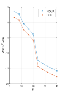
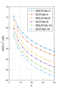
Figure 2: The aggregate error versus the number of devices $K$. (a) SISO scenario. (b) MISO scenario with $N_{d}=4,8,16$. (c) SIMO scenario with $N_{t}=4,8,16$. (d) MIMO scenario with $N_{d}=2,N_{t}=2$, $N_{d}=2,N_{t}=4$, $N_{d}=4,N_{t}=8$.

Simulation results are given in this section to demonstrate the effectiveness of the proposed DLR design and the performance of the proposed near-optimal and closed-form receive beamforming solution when massive antennas are applied. The proposed method is compared with the existing approaches without DRL. The performance of the compared method is labelled as ‘NDLR’ in the SISO and MISO scenarios, which does not optimize the receive beamforming but only optimizes the transmit coefficients (vector) $b_{k}\left(\boldsymbol{b}_{k}\right)$ using the method proposed in [36]. In the SIMO and MIMO scenarios, the SDR and DC methods are compared to obtain receive beamforming vector $\boldsymbol{m}$, which are labelled as ‘SDR’ and ‘DC’. It should be noted that all the devices participate in the update of the global model. We set the maximum transmit power of each device $k$ as $P_{k}=0$ dB, which experiences independent Rayleigh fading. To show the impact of DLR on the training and inference performance, we use FL to implement the classification tasks on MNIST and CIFAR10 datasets. Assume that the data stored at each device has equal size. To ensure that the algorithm has adequate supplies of data to support feature extraction and meaningful learning, $K\geq 20$ has to be satisfied. MLP and ResNet18 neural networks are adopted to train on these two datasets for $200$ epochs, where $\mu$ is set to $0.01$.

VII-A Performance on MSE using DLR

To showcase the effectiveness of the proposed DLR, we conduct simulations under the SISO, MISO, SIMO and MIMO scenarios, where the boundaries of DLR are set to $r_{\min}=1/1.2$ and $r_{\max}=1/0.8$. Fig. 2 displays $\mathrm{MSE}/\sigma^{2}$ with respect to the number of devices $K$. It shows that the aggregate error decreases with the increase of device number $K$ in four scenarios, which is due to the averaging operation over $K$ devices. Specifically, more devices indicate smaller scaling factor $\eta$ and therefore smaller error from (8). The aggregate error is further reduced by additionally considering DLR, compared to the methods utilizing only on wireless resource in [36, 27], which validates Theorem 2 and Theorem 3. It also reveals that performance gap extended with the increase of the number of devices $K$. The reason behind is that the increase of $K$ lead to a larger difference between the maximum and minimum signal power. Compared with the SISO scenario, multiple antennas at the devices or/and the aggregator offer diversity gain to combat fading. Thereby, more antenna deployment results in a smaller aggregate error while the performance gain obtained by DLR is shrinking.

Figure 3: The optimality of the proposed iterative method.

To showcase the optimality of the proposed iterative algorithm, we conduct numerical simulations to obtain the near-optimal solution in the MIMO scenario, as problem (23) is nonconvex and the optimal solution is difficult to obtain. Note that the near-optimal solution is obtained by initializing $10$ starting points and selecting the one with the minimum MSE. Fig. 3 reveals that the proposed iterative learning rate and receive beamforming algorithm can achieve relatively close performance with the near-optimal solution. In order to examine the impact of DLR, we show the channel gain/equivalent channel power and the corresponding DLR values in Fig. 4. For clear illustration, the devices are indexed by the channel gain/equivalent channel gain in an ascending order. As displayed in Fig. 4, the learning rate $\mu_{k}=r_{k}\mu$ is smaller for device $k$ with higher channel gain/equivalent channel gain, while a larger learning rate is used for the local model update with lower channel gain/equivalent channel gain, which can be explained using (9).

Figure 4: The equivalent channel power and the corresponding DLR. (a) MISO scenario with $N_{d}=8$, (b) MIMO scenario with $N_{d}=4,N_{t}=4$.

Simulations are conducted on different boundaries of DLR ratios, i.e., $r_{\mathrm{min}}$ and $r_{\mathrm{max}}$, under four scenarios to illustrate their impact. Note that the case of $r_{\mathrm{min}}=r_{\mathrm{max}}=1$ is equivalent to conventional methods without considering DLR. Fig. 5 shows that a larger range of DLR ratio leads to the decreasing trend of MSE. In Fig. 5(c) and Fig. 5(d), the performance in the cases of $1/r_{\max}=0.4,1/r_{\min}=1.6$ and $1/r_{\max}=0.6,1/r_{\min}=1.4$ is close when $K\leq 10$. Recall that the DLR is inversely proportional with the equivalent channel gain. Such close performance can be explained by the reason that the obtained receive beamforming vector $\boldsymbol{m}$ can well combat the distortion due to the fading channels when $K$ is small.

Figure 5: The impact of $r_{\max}$ and $r_{\min}$. (a) SISO scenario. (b) MISO scenario with $N_{d}=4$. (c) SIMO scenario with $N_{t}=4$. (d) MIMO scenario with $N_{d}=2,N_{t}=2$.

VII-B Performance of Learning Task Using DLR

To investigate the impact of DLR on the training and testing performance of FL tasks, we utilize FL to perform classification tasks on MNIST and CIFAR10 datasets. Fig. 6 gives the training loss as well as the test accuracy on both datasets. $K=20$ devices are involved in updating the global model, and the parameter $a$ and the noise power $\sigma^{2}$ are respectively set to $10$ dB and $0$ dB. Compared to CIFAR10 including $10$ classes of color pictures, MNIST dataset comprising only black and white pictures is known to be much more easier to learn. Thus, the accuracy trained on the MNIST can achieve $90\%$ very soon and approach almost $100\%$, while the accuracy on CIFAR10 is lower with approximate $72\%$. Since the MSE with DLR is smaller than the MSE with a fixed learning rate, its re-transmission probability is smaller. The DLR-based scheme is shown to have slight higher test accuracy on both datasets compared to conventional methods using a fixed learning rate, i.e., $r_{\mathrm{min}}=r_{\mathrm{max}}=1$. This is due to the fact that a increased learning rate owing to adaption to the fading channels can help escape the saddle point which is known as the difficulty in minimizing the loss. In addition, a larger range of DLR may result in a bigger variance of the training loss and the test accuracy, which implies that proper boundaries of DLR ratio should be chosen.

Further numerical simulations are conducted under the MISO and MIMO scenarios with $K=4,12,20$ devices, where $N_{d}=4$, and $N_{d}=2,N_{t}=4$, respectively. The DLR ratio boundaries are set to $r_{\min}=1/1.2$ and $r_{\max}=1/0.8$ , and the noise power is set to $10$ dB. The reported accuracy performance on both datasets is given in Table VII-B. The assumption of sufficient data suggests that the total size of data under $K=4$ and $K=12$ cases is insufficient. As a result, the test accuracy on both datasets is lower when $4$ and $12$ devices participate in aggregating the global model, compared with $20$ devices. It is worth noting that the reported accuracy using DLR may be smaller than that with a fixed learning rate due to the variance. Therefore, the simulation results in Fig. 6 and Table VII-B demonstrate that the proposed DLR can slightly improve the learning and inference performance compared with the fixed-learning-rate-based approach.

Figure 6: The training and testing performance with different $r_{\mathrm{max}}$ and $r_{\mathrm{min}}$. (a) Training loss on MNIST dataset. (b) Accuracy performance on MNIST dataset. (c) Training loss on CIFAR10 dataset. (d) Accuracy performance on CIFAR10 dataset.

TABLE I: Reported accuracy on MNIST and CIFAR10 with $200$ epochs under MISO and MIMO scenarios.

Scenario	Number of devices	$K=4$		$K=12$		$K=20$
	Dataset	MNIST	CIFAR10	MNIST	CIFAR10	MNIST	CIFAR10
MISO $N_{d}=4$	Fixed learning rate	91.12%	53.11%	96.26%	62.68%	97.01%	68.72%
	DLR	93.29%	50.27%	96.35%	64.68%	97.17%	72.12%
MIMO $N_{d}=2$, $N_{t}=4$	Fixed learning rate	93.11%	50.96%	96.71%	63.39%	96.98%	71.29%
	DLR	93.90%	54.86%	96.66%	64.94%	96.94%	73.86%

VII-C Performance of the Proposed Closed-form Receive Beamforming Solution

Now we move on to discuss the impact of the number of antennas on the MSE performance and verify the asymptotic analysis and the proposed closed-form receive beamforming design. Different numbers of antennas at the devices and the aggregator under the MISO, SIMO and MIMO scenarios are considered. Due to the lack of space, we restrict ourselves to the case of $K=2$ and $K=4$ only. The line labeled as ‘Analysis’ is the derived theoretical MSE, and ‘Proposed’ is the performance using the proposed simple closed-form receive beamforming design.

As shown in Fig. 7, the increase of the number of antennas leads to a reduction of aggregate error since higher beamforming gain is achieved. The performance gap shrinks between the proposed DLR and fixed learning rate methods for $r_{k}\rightarrow 1$ when the number of antennas go to infinity. More specifically, in the MISO scenario, more antennas equipped at the devices lead to smaller differences on the channel gain among devices. Thus the performance gain obtained by DLR is smaller with respect to fixing learning rate. Both ‘DLR’ and ‘NDLR’ approach the ‘Analysis’ performance eventually, which verifies the analysis under the MISO case. In the SIMO and MIMO scenarios, more antennas at the aggregator provide more freedom to align the received signals, which leads to the reduced performance gap between ‘DLR’ and ‘DC’.

Fig. 7 also shows that the MSE obtained by the proposed closed-form receive beamforming design is approaching the theoretical bound when massive antenna are applied. Besides, the MSE without consideration of DLR, i.e., ‘NDLR’ in the MISO case and ‘DC’ in both SIMO and MIMO cases, is getting closer to ‘Analysis’, which implies that the equality of (a) and (b) in both (28) and (34) are guaranteed. Based on the theoretical analysis in Section VI, when the the number of receive antennas (or transmit antennas) goes to infinity, the analyzed MSE is the same for both MIMO and MISO (or SIMO). From Fig. 7 we observe that the number of transmit (or receive) antennas can affect the changing rate of MSE curve when the number of the receive (or transmit) antennas goes to infinity. Therefore, the asymptotic analysis is verified and the effectiveness of the proposed closed-form receive beamforming design in Section VI is confirmed.

Figure 7: The impact of antenna number and the performance of the proposed closed-form receive beamforming design. (a) MISO scenario. (b) SIMO scenario. (c) MIMO scenario with $N_{t}=2$. (d) MIMO scenario with $N_{d}=2$.

VIII Conclusions

In this paper, we incorporated the Aircomp technique in implementing distributed learning tasks to significantly improve the communication efficiency. Minimizing the aggregate error due to the fading and noisy channels is critical as a large error can lead to poor training and inference performance. Different from existing works that mainly optimized the wireless resources to align the received signals, we first proposed to utilize optimizable learning rates and proposed DLR to adapt to the fading channels. The problem was formulated under the MISO and MIMO scenarios. A closed-form solution and an iterative method were proposed respectively for each case. The simulation results have validated the effectiveness of the proposed DLR in terms of both the MSE performance and the testing accuracy on the MNIST and CIFAR10 datasets. Asymptotic analyses in the MISO, SIMO and MIMO scenarios were also provided to address the problem of massive antenna deployment as well as to derive the theoretical bounds. On this basis, a near-optimal and closed-form receive beamforming design was proposed by simply summing up the channel vectors. The feasibility and effectiveness of the proposal are verified by extensive numerical simulations.

References

- [1] K. B. Letaief, W. Chen, Y. Shi, J. Zhang, and Y. A. Zhang, “The roadmap to 6G: AI empowered wireless networks,” IEEE Commun. Mag., vol. 57, no. 8, pp. 84–90, Aug. 2019.
- [2] Y. Huang, S. Liu, C. Zhang, X. You, and H. Wu, “True-data testbed for 5G/B5G intelligent network,” Intell. Converged Networks, 2021, in press.
- [3] W. Saad, M. Bennis, and M. Chen, “A vision of 6G wireless systems: Applications, trends, technologies, and open research problems,” IEEE Network, vol. 34, no. 3, pp. 134–142, May 2020.
- [4] C. Zhang, P. Patras, and H. Haddadi, “Deep learning in mobile and wireless networking: A survey,” IEEE Commun. Surv. Tutorials, vol. 21, no. 3, pp. 2224–2287, Mar. 2019.
- [5] C. Xu, S. Liu, C. Zhang, Y. Huang, Z. Lu, and L. Yang, “Multi-agent reinforcement learning based distributed transmission in collaborative cloud-edge systems,” IEEE Trans. Veh. Technol., 2021, in press.
- [6] S. Dang, O. Amin, B. Shihada, and M.-S. Alouini, “What should 6G be?” Nat. Electron., vol. 3, no. 1, pp. 20–29, Jan. 2020.
- [7] M. Chen, U. Challita, W. Saad, C. Yin, and M. Debbah, “Artificial neural networks-based machine learning for wireless networks: A tutorial,” IEEE Commun. Surv. Tutorials, vol. 21, no. 4, pp. 3039–3071, Jul. 2019.
- [8] S. Bi, R. Zhang, Z. Ding, and S. Cui, “Wireless communications in the era of big data,” IEEE Commun. Mag., vol. 53, no. 10, pp. 190–199, Oct. 2015.
- [9] G. Zhu, D. Liu, Y. Du, C. You, J. Zhang, and K. Huang, “Toward an intelligent edge: Wireless communication meets machine learning,” IEEE Commun. Mag., vol. 58, no. 1, pp. 19–25, Jan. 2020.
- [10] J. Park, S. Samarakoon, M. Bennis, and M. Debbah, “Wireless network intelligence at the edge,” Proc. IEEE, vol. 107, no. 11, pp. 2204–2239, Oct. 2019.
- [11] B. McMahan, E. Moore, D. Ramage, S. Hampson, and B. A. y Arcas, “Communication-efficient learning of deep networks from decentralized data,” in Proc. Int. Conf. Artif. Intell. Stat. (AISTATS), Fort Lauderdale, FL, USA, Apr. 2017, pp. 1273–1282.
- [12] Y. Liu, X. Yuan, Z. Xiong, J. Kang, X. Wang, and D. Niyato, “Federated learning for 6G communications: Challenges, methods, and future directions,” China Commun., vol. 17, no. 9, pp. 105–118, Sept. 2020.
- [13] Z. Yang, M. Chen, K.-K. Wong, H. V. Poor, and S. Cui, “Federated learning for 6G: Applications, challenges, and opportunities,” 2021. [Online]. Available: https://arxiv.org/abs/2101.01338
- [14] P. M, S. P. R. M, Q.-V. Pham, K. Dev, P. K. R. Maddikunta, T. R. Gadekallu, and T. Huynh-The, “Fusion of federated learning and industrial internet of things: A survey,” 2021. [Online]. Available: https://arxiv.org/abs/2101.00798
- [15] Q. Zhou, S. Guo, H. Lu, L. Li, M. Guo, Y. Sun, and K. Wang, “Falcon: Addressing stragglers in heterogeneous parameter server via multiple parallelism,” IEEE Trans. Computers, vol. 70, no. 1, pp. 139–155, Feb. 2021.
- [16] W. Wen, C. Xu, F. Yan, C. Wu, Y. Wang, Y. Chen, and H. Li, “Terngrad: Ternary gradients to reduce communication in distributed deep learning,” in Proc. Int. Conf. Neural Inf. Process. Syst. (NIPS), Long Beach, CA, USA, Dec. 2017, pp. 1508–1518.
- [17] D. Alistarh, D. Grubic, J. Z. Li, R. Tomioka, and M. Vojnovic, “QSGD: Communication-efficient SGD via gradient quantization and encoding,” in Proc. Int. Conf. Neural Inf. Process. Syst. (NIPS), Long Beach, CA, USA, Dec. 2017, pp. 1707–1718.
- [18] Y. Lin, S. Han, H. Mao, Y. Wang, and B. Dally, “Deep gradient compression: Reducing the communication bandwidth for distributed training,” in Proc. Int. Conf. Learn. Representations (ICLR), Vancouver, BC, Canada, May 2018.
- [19] A. Aji and K. Heafield, “Sparse communication for distributed gradient descent,” in Proc. Conf. Empirical Methods Natural Language Process. (EMNLP), Copenhagen, Denmark, Sept. 2017, pp. 440–445.
- [20] T. Nishio and R. Yonetani, “Client selection for federated learning with heterogeneous resources in mobile edge,” in Proc. IEEE Int. Conf. Commun. (ICC), Shanghai, China, May 2019, pp. 1–7.
- [21] J. Ren, G. Yu, and G. Ding, “Accelerating DNN training in wireless federated edge learning systems,” IEEE J. Sel. Areas Commun., vol. 39, no. 1, pp. 219–232, Jan. 2021.
- [22] H. H. Yang, Z. Liu, T. Q. S. Quek, and H. V. Poor, “Scheduling policies for federated learning in wireless networks,” IEEE Trans. Commun., vol. 68, no. 1, pp. 317–333, Jan. 2020.
- [23] G. Zhu, J. Xu, K. Huang, and S. Cui, “Over-the-air computing for wireless data aggregation in massive IoT,” 2020. [Online]. Available: https://arxiv.org/abs/2009.02181
- [24] M. Mohammadi Amiri and D. Gündüz, “Machine learning at the wireless edge: Distributed stochastic gradient descent over-the-air,” IEEE Trans. Signal Process., vol. 68, pp. 2155–2169, Mar. 2020.
- [25] M. M. Amiri and D. Gündüz, “Federated learning over wireless fading channels,” IEEE Trans. Wireless Commun., vol. 19, no. 5, pp. 3546–3557, May 2020.
- [26] G. Zhu, Y. Wang, and K. Huang, “Broadband analog aggregation for low-latency federated edge learning,” IEEE Trans. Wireless Commun., vol. 19, no. 1, pp. 491–506, Jan. 2020.
- [27] K. Yang, T. Jiang, Y. Shi, and Z. Ding, “Federated learning via over-the-air computation,” IEEE Trans. Wireless Commun, vol. 19, no. 3, pp. 2022–2035, Mar. 2020.
- [28] D. Yu, S. H. Park, O. Simeone, and S. S. Shitz, “Optimizing over-the-air computation in IRS-aided C-RAN systems,” in Proc. IEEE 21st Int. Workshop Signal Process. Advances Wireless Commun. (SPAWC), Atlanta, GA, USA, May 2020, pp. 1–5.
- [29] W. Ni, Y. Liu, Z. Yang, H. Tian, and X. Shen, “Federated learning in multi-RIS aided systems,” 2020. [Online]. Available: https://arxiv.org/abs/2010.13333
- [30] G. B. Orr and K.-R. Müller, Neural networks: Tricks of the trade. Springer, 2003.
- [31] C. Darken, J. Chang, J. Moody et al., “Learning rate schedules for faster stochastic gradient search,” in Proc. IEEE Workshop Neural Networks Signal Process., Helsingoer, Denmark, Sept. 1992, pp. 3–12.
- [32] S. Ruder, “An overview of gradient descent optimization algorithms,” 2016. [Online]. Available: https://arxiv.org/abs/1609.04747
- [33] L. N. Smith, “Cyclical learning rates for training neural networks,” in Proc. IEEE Winter Conf. Appl. Comput. Vision (WACV), Santa Rosa, CA, USA, Mar. 2017, pp. 464–472.
- [34] G. Zhu and K. Huang, “Mimo over-the-air computation for high-mobility multimodal sensing,” IEEE Internet Things J., vol. 6, no. 4, pp. 6089–6103, Aug. 2019.
- [35] M. Chen, Z. Yang, W. Saad, C. Yin, H. V. Poor, and S. Cui, “A joint learning and communications framework for federated learning over wireless networks,” 2019. [Online]. Available: https://arxiv.org/abs/1909.07972
- [36] L. Chen, X. Qin, and G. Wei, “A uniform-forcing transceiver design for over-the-air function computation,” IEEE Wireless Commun Lett., vol. 7, no. 6, pp. 942–945, Dec. 2018.
- [37] Z. Luo, W. Ma, A. M. So, Y. Ye, and S. Zhang, “Semidefinite relaxation of quadratic optimization problems,” IEEE Signal Process. Mag., vol. 27, no. 3, pp. 20–34, May 2010.
- [38] J. Y. Gotoh, A. Takeda, and K. Tono, “DC formulations and algorithms for sparse optimization problems,” Math. Program., vol. 169, no. 1, pp. 141–176, May 2018.