Does Collateral Value Affect Asset Prices?
Evidence from a Natural Experiment in Texas

Abstract

Does the ability to pledge an asset as collateral, after purchase, affect its price? This paper identifies the impact of collateral service flows on house prices, exploiting a plausibly exogenous constitutional amendment in Texas that legalized home equity loans in 1998. The law change increased Texas house prices 4%; this is price-based evidence that households are credit-constrained and value home equity loans to facilitate consumption smoothing. Prices rose more in locations with inelastic supply, higher prelaw house prices, higher income, and lower unemployment. These estimates reveal that richer households value the option to pledge their home as collateral more strongly. (JEL R0, R3, G0, E21, E44, G2)

1 Introduction

Real estate is the largest source of collateral used by American households (FRBNY, 2016). A home can be pledged as collateral for a loan at the time of purchase or after purchase via a home equity loan (HEL). Theory predicts that an asset’s price should reflect all of its benefits including options to pledge it as collateral. This paper seeks to quantify if the ability to pledge an asset as collateral, after purchase, affects the price.

Prior to 1998, a home in Texas could only be pledged as collateral for a purchase mortgage or home improvement loan. Beginning in 1998, Proposition 8 (a Texas constitutional amendment inspired by federal tax reform and a circuit court ruling) greatly expanded the set of mortgages available to Texans. Texas homeowners gained access to HELs, cash-out refinance loans, and reverse mortgages; however, the total value of all new liens on the home after purchase could not exceed 80% of its appraised price. Because Texas was the only state with such restrictions, this law change provides a unique source of exogenous variation; it expanded future debt capacity (allowing homeowners to extract home equity via HELs) without affecting purchase debt capacity (the amount homebuyers could borrow at purchase was unaffected).

While many papers study the impact of home equity borrowing on consumption and investment (Section 1.1), the current paper examines the impact on house prices. There are three related questions. First, what was the total impact of the law change on house prices? Second, which locations were more affected? Third, what was the mechanism through which the law change affected house prices? The law change could have raised house prices directly through demand for collateral service flows or indirectly by affecting other variables related to house prices. The identifying assumption behind the first question, the causal effect, is that the law change was exogenous conditional on fixed effects and controls. The identifying assumption behind the direct mechanism is that the law change did not affect other variables related to house prices. This paper does not estimate willingness to pay for the embedded option to pledge a home as collateral.

This paper exploits this plausibly exogenous law change to identify the impact of collateral service flows on house prices. The estimation requires detailed Texas house price data, which are notoriously hard to access because Texas is a nondisclosure state; recently available house price indexes from the FHFA (17,936 five-digit zip codes), however, make this analysis possible.

Difference-in-differences estimates show that the impact of the HEL legalization on Texas house prices was positive. The law change raised Texas house prices 4.13%. This result is robust across specifications and sample restrictions. There is no evidence of an effect before implementation. In addition, synthetic control estimates find similar effects in Texas zip codes and no evidence of a placebo effect in untreated zip codes in border states.

The treatment effect was heterogeneous along several dimensions. Consistent with theory, the effect was smaller in elastic locations (where it is relatively easy to build); each unit of the Saiz (2010) measure of supply elasticity corresponds to a 0.9% lower rise in prices. Furthermore, zip codes with higher prelaw house prices, higher income, and lower unemployment rates saw a greater rise in prices, indicating that households in richer locations valued this option more. While it has been shown that an expansion in purchase mortgage debt capacity has a greater impact on ex ante lower-priced properties (Landvoigt et al., 2015), this paper shows that an expansion in future HEL debt capacity has a greater impact on ex ante higher-priced properties. This can be explained by (1) the greater tax shield available to rich households, (2) the tendency of rich households to be more financially literate and aware of these financial products (Lusardi and Mitchell, 2014), and (3) the tendency of rich households to be more likely to qualify for HELs as they tend to have better credit and more stable income (DeFusco and Mondragon, 2018).

The heterogeneity analysis refines the interpretation of the main result. The impact of HEL legalization on house prices is not just a measure of the extent to which households expect to be credit-constrained, but also a measure of the extent to which households expect to qualify for HELs to smooth consumption. For example, a recently unemployed homeowner may want to borrow but not qualify for a HEL. On the other hand, a homeowner with high stable income (hence a high marginal tax rate) and good credit is more likely to be approved for a bigger loan at a lower effective interest rate.

The mechanism through which HEL legalization increased house prices could have occurred through two broad types of channels:

1. Direct Channel: the law caused a rise in demand for owner-occupied housing due to the new option allowing homes to be pledged as collateral after purchase.

2. Indirect Channel: the law affected other variables that affect house prices. For example, if the law increased investment enough to stimulate the local economy, this increase could have raised demand for housing, consequently raising the price.

The mechanism is investigated in two ways. First, falsification tests show that the law change did not affect observed variables related to prices including rent, population, and income. There was a small (0.3%) but statistically significant rise in unemployment, which works against the indirect channel. Second, estimates in border cities (such as Texarkana) are similar to the bigger samples, providing further support for the direct channel. Border cities are often viewed as one economy. Hence, if the law change stimulated the economy, the indirect channel would affect both the Texas and control sides of the border city, while the direct channel would only affect the Texas side. Together, these results provide evidence that most of the effect was through the direct channel.

Finally, in partial equilibrium the law change should have increased demand for owner-occupied housing relative to renting (in Texas) because owners can pledge their home as collateral but renters cannot. On the other hand, in general equilibrium, the rise in house prices from this law change should have caused a reduction in demand. The net effect of this law change on homeownership is theoretically ambiguous. Estimates show that Texas homeownership rates, single-family building permits, and population were unaffected by the law. These results indicate that house prices rose enough to keep the marginal homebuyer indifferent between owning and renting.

Inference about external validity to the collateral value of other assets, in other locations, at other times should be made with caution. This paper finds that after-purchase collateral service flows had a positive impact on the price of owner-occupied housing in Texas after 1998. The conceptual framework predicts that there should be a positive effect for other assets, in other locations, at other times. In particular, the effect is likely higher for housing in other states, because Texas is the only state with an 80% limit on future home equity extraction. Unfortunately, it is hard to quantify the collateral value of other assets because it is rare to find large discontinuous changes in lending laws.

This paper makes three contributions:

1. It empirically identifies if, and to what extent, the option to pledge a home as collateral, after purchase, affects its price.

2. It provides price-based evidence that households are borrowing-constrained. The treatment effect is a measure of the extent to which households value HELs to facilitate future consumption smoothing.

3. It provides new evidence on the distribution of credit supply. Richer households that get a greater mortgage interest tax shield, are more financially literate, and are more likely to qualify value HELs more strongly.

1.1 Literature review

Many strands of literature study borrowing constraints and collateral. Theoretical literature has shown that frictions such as adverse selection, moral hazard, and the inability to fully pledge future labor income restrict borrowing. Borrowers often pledge collateral to mitigate these frictions.

A second strand of literature studies the relationship between housing, credit constraints, and consumption. Households that are, or fear they will be, credit-constrained should have a stronger demand for assets that facilitate their future ability to borrow. If prices reveal information, the magnitude of the treatment effect estimated in this paper can be interpreted as a measure of the extent to which households value HELs as a tool to relax credit constraints.

A third strand of literature studies the relationship between property prices, firm investment, and entrepreneurship. There is evidence that rises and declines in property values, which affect debt capacity, amplify firm investment in the United States and Japan but not in China. While theory predicts that firms prefer to own assets that serve as better collateral, none of these papers empirically identifies if and to what extent asset prices reflect this.

A fourth strand of literature compares the collateral service flows of different assets. The interest rate borrowers pay in the repo market depends on the type of collateral they use (Bartolini et al., 2010). For example, borrowers who pledge treasuries as collateral often borrow at “special” repo rates. Duffie (1996) showed that “specialness” should raise the price of the underlying security by the present value of interest rate savings. The estimates below can be interpreted through the lens of Duffie (1996): the collateral value of housing should reflect the interest rate savings on a HEL relative to an unsecured loan.

In addition to the interest rate savings, the collateral value should also reflect the greater debt capacity of housing via a lower margin requirement (higher loan-to-value [LTV] ratio) relative to unsecured credit and debt secured by other forms of collateral. In related work, Gârleanu and Pedersen (2011) and Jylhä (2018) showed that a security’s margin also affects its return.

The collateral value of other assets – such as airplanes, cars, fine art, gold, and patents – has also been studied. In particular, Huang and Kilic (2018) argued that gold is a better source of collateral than platinum for historical and institutional reasons. For example, gold is formally recognized as collateral by the Basel Accords and is accepted as collateral by broker dealers, while platinum is not. They contended that, in times when the probability of a consumption disaster is high, agents prefer gold for its collateral benefits, which is reflected in the price. The results in this paper provide support for the “Flight to Collateral” phenomenon (Fostel and Geanakoplos, 2008) as distinct from “Flight to Liquidity”, as homeowners value the collateral privileges of real estate despite its lack of liquidity.

A fifth strand of literature studies the impact of total mortgage leverage (including purchase mortgages) on house prices. In particular, Favilukis et al. (2017) showed that (total) mortgage leverage played a quantitatively important role in explaining the housing boom-bust cycle.

It is worth emphasizing that this paper focuses on nonpurchase mortgage leverage as opposed to total or purchase leverage. A purchase mortgage can be used to buy a house and to otherwise smooth consumption (since money is fungible). The Texas law change studied here did not affect a household’s ability to finance the original purchase, but rather its ability to pledge its home as collateral in the future. There is evidence that HEL debt capacity increased purchase mortgage debt capacity for some households that used second liens (“piggy-back mortgages”) to avoid mortgage insurance and obtain bigger loans (Lee et al., 2013). This was not a relevant factor in Texas because the law included an 80% LTV limit for all liens after purchase.

Note that there is different terminology in the literature for how the ability to pledge an asset as collateral affects its price. Fostel and Geanakoplos (2008) call this the collateral value, Brumm et al. (2015) call this the collateral premium, and He et al. (2015) call this the liquidity premium.

2 Institutional Setting

Texas lending laws have been studied widely in the history, legal, and recently economic literature. Restrictions on mortgage lending existed in Texas before it became a U.S. state. These laws, protecting homes from creditors, carried over to the state’s original constitution in 1845 and to subsequent versions (Internet Appendix E). Before 1998, the Texas constitution protected homes from foreclosure except for nonpayment of property taxes, the purchase mortgage, mechanics’ liens for home improvement, and refinance loans. Under Texas law, refinance loans were only allowed up to the balance, permitting homeowners to get a lower payment (if interest rates fell) but not to borrow an additional amount. Suppose a Texan borrowed $200,000 to buy a home, and five years later the remaining balance was $150,000. If interest rates fell, the Texan could refinance into a new mortgage for at most $150,000. This allowed Texas homeowners to lower their mortgage payments, but not to extract equity (i.e., borrow an additional amount). This was a binding restriction. Chen et al. (2016) find that 61% of all refinance mortgages in the United States are cash-out loans. The fraction of cash-out loans was over 80% in years when the interest rate incentive was high. Before 1998, the only way for a Texas homeowner to extract home equity was to sell the home at substantial transaction costs.

The literature (Internet Appendix E) has linked the movement to amend Texas lending laws to two main factors: federal tax reform and a circuit court ruling. First, the Tax Reform Act of 1986 made mortgage interest the only form of interest on consumer credit that is tax deductible. This tax shield made HELs more attractive than other forms of debt such as auto loans, personal loans, and credit card debt. While HELs expanded throughout the United States after this tax reform, Texans did not have access to this additional tax shield. Second, the Fifth Circuit (with jurisdiction over Louisiana, Mississippi, and Texas) ruled in 1994 that federal regulations superseded the Texas constitution. This temporarily overturned Texas restrictions on HELs. Even though subsequent actions by lawmakers quickly reestablished the restrictions, this ruling brought attention to amending Texas mortgage laws.

Since these lending restrictions were in the Texas constitution, they could only be overturned by a constitutional amendment. This requires a joint resolution from both the state Senate and House. If the resolution is approved with a two-thirds vote in each, it becomes a proposition, which must then be passed by a majority of the state’s voters in a referendum.

Joint Resolution 31, to amend the state constitution and legalize home equity lending, was passed by the Texas House and Senate in May 1997. This resulted in Proposition 8, which was approved by Texas voters in November 1997. The amendment became effective January 1, 1998, legalizing after-purchase mortgages with a combined balance of up to 80% of the appraised market value of the home. Suppose that after 1998, a Texan’s home was appraised to be worth $200,000, and the original purchase mortgage had an outstanding balance of $100,000. The homeowner could borrow up to 80% $\times$ $200,000 =$160,000 and get a second lien HEL (or reverse mortgage) for up to $60,000 or a cash-out refinance loan for up to $160,000.

There is evidence in the literature that Texans took advantage of these newly available products after Proposition 8 was passed. Abdallah and Lastrapes (2012) showed that Texans took out home equity loans, and Kumar (2018) showed that Texans used cash-out refinance loans.

3 Conceptual Framework

This section constructs a model to help interpret the results below. The model has three main goals: (1) to illustrate how pledgeability affects the standard asset pricing equation, (2) to study the heterogeneity of collateral service flows, (3) to clarify the different mechanisms through which collateral service flows affect house prices. Consider a household that values nondurable consumption $c_{t}$ and durable housing $h_{t}$, which depreciates at rate $\delta_{t}$. The household can borrow up to $\kappa_{t}\equiv\min\left\{\overline{\kappa}_{t},LTV_{t}\right\}$ of its house value, where $\overline{\kappa}_{t}$ is the legal limit and $LTV_{t}$ is the most lenders will lend at time $t$. It solves

$$\max\text{ }\mathbb{E}_{0}\sum_{t=0}^{\infty}\beta^{t}u(c_{t},h_{t})$$ s.t.

$$c_{t}+p_{t}h_{t+1}+a_{t+1} \leq y_{t}+p_{t}h_{t}(1-\delta_{t})+(1+r_{t})a_{t} \lambda_{t}$$ (DBC )

$$-a_{t+1} \leq\kappa_{t}p_{t}h_{t} \mu_{t}$$ (CC )

where $u(c_{t},h_{t})$ is the household’s flow utility from consumption and housing, assumed twice continuously differentiable and strictly concave in each argument. $\lambda_{t}$ is the multiplier on the dynamic budget constraint (DBC) and $\mu_{t}$ is the multiplier on the collateral constraint (CC). $c_{t}$ is the numéraire, and $p_{t}$ is the price per unit of housing. $a_{t}$ is the amount saved or borrowed at interest rate $r_{t}$, and $y_{t}$ is income.

The solution to the household’s problem (derived in Appendix F) reveals that house prices reflect service flows from shelter and collateral:

$$\underbrace{p_{t}}_{\text{price}} =\mathbb{E}_{t}\left[\underbrace{\beta\frac{u_{c}(t+1)}{u_{c}(t)}}_{\text{ discount factor}}\times\left(\underbrace{\frac{u_{h}(t+1)}{u_{c}(t+1)}}_{\begin{subarray}{c}\text{housing}\\ \text{service flow (rent)}\end{subarray}}+\underbrace{\frac{\mu_{t+1}\kappa_{t+1}p_{t+1}}{u_{c}(t+1)}}_{\begin{subarray}{c}\text{collateral}\\ \text{service flow}\end{subarray}}+\underbrace{(1-\delta_{t+1})p_{t+1}}_{\text{resale price}}\right)\right]$$ (1a)

$$\mu_{t+1} =u_{c}(t+1)-\mathbb{E}_{t+1}[\beta\left(1+r_{t+2}\right)u_{c}(t+2)]$$ (1b)

Equations (1a) and (1b) come from the first-order conditions (FOCs). Following Favilukis et al. (2017), the periodic service flow from housing can be interpreted as a cash flow equal to rent. If a household is credit-constrained, then $\mu_{t+1}>0$, and its FOCs reflect the collateral service flow. Any model with a collateral constraint has this type of collateral term (denoted $CSF_{t}$). Even though it is ubiquitous, it is hard to quantify, as it is rare to find a setting with a large exogenous shock to the pledgeability of housing $\kappa_{t}$.

In equilibrium, the only way the collateral service flow can be positive is if there is at least one unconstrained household that is lending with $\mu_{t+1}=0$. Hence a general equilibrium model requires heterogeneity for $CSF_{t+1}>0$. A convenient way to model this heterogeneity is with an impatient borrower and a patient lender (Iacoviello, 2005; Kiyotaki and Moore, 1997). An alternative way to model positive collateral service flow is to allow interest rates to be exogenous and to assume the representative agent borrows from a deep-pocket, risk-neutral, international lender (Bianchi et al., 2012).

The results above can help illustrate heterogeneity in the collateral service flow. First, index each household with superscript $j$. Second, rewrite the effective interest rate for household $j$ as $r_{t}^{j}=(1-\tau_{t}^{j})i_{t}^{j}$, where $\tau_{t}^{j}$ is household $j$’s marginal income tax rate and $i_{t}^{j}$ is the contract rate charged to household $j$. Finally, index household $j$’s credit constraint $\kappa_{t}^{j}\equiv\min\left\{\overline{\kappa}_{t},LTV_{t}^{j}\right\}$. Note that (1) households with higher marginal income tax rates $\tau_{t}^{j}$ enjoy a bigger mortgage interest deduction and (2) different households are charged different interest rates and credit limits depending on their risk (measured by their credit score and stability of income). The collateral service flow for household $j$ can be decomposed from Equations (1a) and (1b):

$$\underbrace{CSF_{t}^{j}}_{\begin{subarray}{c}\text{collateral}\\ \text{service flow}\end{subarray}} =\frac{1}{u_{c}(t)}\times\underbrace{\mu_{t}^{j}}_{\text{desire to borrow}}\times\underbrace{\kappa_{t}^{j}}_{\text{fraction you can borrow}}\times\underbrace{p_{t}}_{\text{value of collateral}}$$ (2a)

$$=\frac{1}{u_{c}(t)}\times\left(u_{c}(t)-\mathbb{E}_{t}[\beta\left(1+(1-\tau_{t}^{j})i_{t}^{j}\right)u_{c}(t+1)]\right)\times\kappa_{t}^{j}\times p_{t}$$ (2b)

This decomposition shows that the value of being able to pledge housing as collateral depends on the desire to borrow $\mu_{t}^{j}$ and the debt capacity $\kappa_{t}^{j}p_{t}$ (the amount a homeowner can borrow), which depends on $j^{\prime}s$ access to credit.

The component $\mu_{t}^{j}$ (the multiplier on the collateral constraint) is a measure of the desire to borrow. If there is no demand for HELs (or if markets are complete), then $\mu_{t}^{j}=0$, making $CSF_{t}^{j}=0$. The collateral service flow can still affect property prices today if there is a desire for HELs in the future. Observe from equation 2b that the desire to borrow depends negatively on the effective interest rate that household $j$ faces. Households that face lower effective interest rates (because they have better credit scores or more stable documented income) should have a greater demand for HELs. The estimates in Section 5.3 are consistent with this prediction.

The component $\kappa_{t}^{j}\equiv\min\left\{\overline{\kappa}_{t},LTV_{t}^{j}\right\}$ depends on (a) the amount households can legally borrow $(\overline{\kappa}_{t})$ and (b) the amount lenders are willing to lend $(LTV_{t}^{j})$. If HELs are illegal $\left(\overline{\kappa}_{t}=0\right)$, equation 2a implies $CSF_{t}=0$, as in Texas before 1998. Abdallah and Lastrapes (2012) and Kumar (2018) showed that HELs and cash-out refinance loans were indeed utilized by Texans after 1998. It is worth noting that the amount lenders are willing to lend, $LTV_{t}^{j}$, depends on the borrower’s characteristics: borrowers with better credit scores and stable documented income are more likely to qualify for bigger loans (Brueggeman and Fisher, 2011). These underwriting requirements help explain the heterogeneity results in Section 5.3.

The model above does not distinguish between the ability to pledge an asset as collateral at the time of purchase and in the future. Appendix G considers a three-period setting where purchase mortgage collateral service flows are disentangled from HEL collateral service flows. In this setting, the borrower’s HEL debt capacity is equal to $\kappa_{t}p_{t}h_{t}-B_{t}^{pm}$, where $B_{t}^{pm}$ is the remaining balance on the purchase mortgage used to buy the home. For example, consider a household that owns a home appraised to be worth $p_{t}h_{t}=\$100k$ with a remaining balance on its purchase mortgage of $B_{t}^{pm}=\$50k$. If this household can borrow up to $\kappa_{t}=80\%$ of the price, then its HEL debt capacity would be $80\%\times\$100k-\$50k=\$30k$.

4 Empirical Strategy, Identification, and Data

4.1 Empirical strategy

This paper estimates the impact of the HEL legalization on various outcome variables with a generalized difference-in-differences (DID) methodology. The main analysis uses four geographically nested samples (United States, Border-State, Border, and CBCP), explained below. Four border cities (notably Texarkana) are also studied. Further analysis constructs a synthetic control group for each treated zip code and conducts placebo tests for untreated zip codes. In all samples, the treated group consists of all locations in Texas and the control group includes all locations outside Texas. The U.S. sample includes all zip codes with data six years before and after the treatment year, 1998. The Border State sample restricts the U.S. sample to all zip codes in Texas and its border states (Louisiana, Arkansas, Oklahoma, and New Mexico). The Border sample restricts the Border State sample to all zip codes within a 50-mile radius of each Texas zip code, using distance data from the NBER and Census. Only zip codes that include both Texas and non-Texas locations within a 50-mile radius are kept. The fourth, and most local, sample is the Contiguous Border County Pair (CBCP) sample. This sample consists of all zip codes that belong to a contiguous county on either side of the Texas border. Since a given Texas county may border more than one non-Texas county, data in this sample are stacked as in Dube et al. (2010), making it possible to identify county pair by year fixed effects.

The local samples can help control for unobserved heterogeneity to the extent that houses near each other are more likely to be affected by the same local shocks such as hurricanes and factory shutdowns. In particular, the border city Texarkana, the only Metropolitan Statistical Area (MSA) in Texas that includes another state, can be viewed as one economy. So if the law change affected the economy on the Texas side of Texarkana, it should have also affected the economy on the Arkansas side.

This paper estimates:

$$y_{i,s,t} =\alpha_{i}+\theta_{t}+{\color[rgb]{.5,0,.5}\beta_{DID}}Texas_{s}\times Post_{t}+\Gamma X_{i,s,t}+\varepsilon_{i,s,t}$$ (static DID)

$$y_{i,s,t} =\alpha_{i}+\theta_{t}+\sum_{k\neq 1997}{\color[rgb]{.5,0,.5}\eta_{k}}Texas_{s}\times 1_{k}+\Gamma X_{i,s,t}+\varepsilon_{i,s,t},$$ (dynamic DID)

where $y_{i,s,t}$ is the outcome variable. In the main regressions, it is the log real house price index. In further regressions, real house price growth, log real rent, log population, log real income per capita, unemployment rate, homeownership rate, and log single-family building permits are also considered. The index $i$ corresponds to the most local level of the outcome variable. For house price regressions, $i$ is the zip code. For population, income, employment, and permit regressions, $i$ is the county Federal Information Processing Standard (FIPS) code. For rent and homeownership rate regressions, $i$ is the MSA. The index $s$ corresponds to the level of treatment, which is the state in all regressions. $Texas_{s}$ is the treatment group indicator variable, which is equal to $1$ if $s=Texas$. $Post_{t}$ is the treatment period indicator variable, which is equal to $1$ for $t\geq 1998$. $1_{k}$ is a year indicator variable, which is equal to $1$ for $t=k$. $\alpha_{i}$ and $\theta_{t}$ are the location and time fixed effects. $\varepsilon_{i,s,t}$ is an error term assumed to be conditionally uncorrelated with the treatment.

Specifications in the main analysis include location fixed effects, time fixed effects, time trends, and national oil prices interacted with MSA dummies. The CBCP sample also includes county pair by year fixed effects. Robustness tests also consider national interest rates interacted with state dummies as well as real income per capita and population.

This paper also investigates heterogeneity in the treatment effect – that is, whether the law change had a different impact in different locations. To study the sensitivity of the effect to various observable measures of heterogeneity $H_{i}$, this paper estimates:

$$y_{i,s,t} =\alpha_{i}+\theta_{t}+{\color[rgb]{.5,0,.5}\beta_{H,0}}Texas_{s}\times Post_{t}+\beta_{5}Texas_{s}\times H_{i}+\beta_{6}Post_{t}\times H_{i}$$

$$+{\color[rgb]{.5,0,.5}\beta_{H}}Texas_{s}\times Post_{t}\times H_{i}+\Gamma X_{i,s,t}+\varepsilon_{i,s,t}$$ (DDD)

In this specification, the average treatment effect (ATE) is an affine function of $H_{i}$:

$$\text{ATE}\left(H_{i}\right) ={\color[rgb]{.5,0,.5}\beta_{H,0}}+{\color[rgb]{.5,0,.5}\beta_{H}}H_{i}$$

The coefficient ${\color[rgb]{.5,0,.5}\beta_{H,0}}$ is the estimated average treatment effect if $H_{i}=0$, and ${\color[rgb]{.5,0,.5}\beta_{H}}=\frac{\partial\text{ATE}\left(H_{i}\right)}{\partial H_{i}}$ is the sensitivity of the average treatment effect to a rise in $H_{i}$.

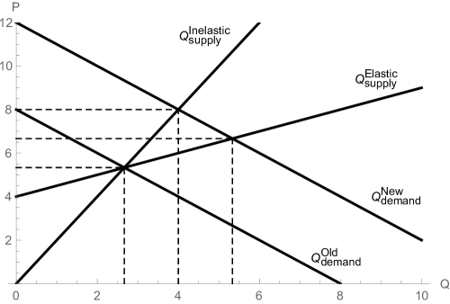
Figure 4: The impact of a rise in demand on house prices in cities with different supply elasticities

For example, theory predicts that a rise in demand should have a smaller impact on house prices in elastically supplied locations where it is easier to build real estate (Figure 4). This corresponds to the hypothesis ${\color[rgb]{.5,0,.5}\beta_{elasticity}}<0$. The coefficient ${\color[rgb]{.5,0,.5}\beta_{elasticity,0}}$ is the estimated impact of the law change on prices in a hypothetical location where the asset (housing) is in perfectly inelastic supply.

This paper investigates treatment effect heterogeneity in elasticity, prelaw median house prices, income, and unemployment. Prelaw variables are set equal to their average value before 1998 to ensure they are unaffected by the treatment.

4.2 Identification

The main goal of this paper is to identify the impact of the HEL legalization on house prices. The identifying assumption is that the error term is conditionally uncorrelated with the treatment. The identifying assumption can be defended because the constitutional amendment, approved by the state House, Senate, and ultimately by Texas voters in a referendum, was motivated by federal tax reform and a circuit court ruling (Section 2). These factors are not linked to Texas house prices and other outcome variables studied in this paper. Forrester (2002) reviews the extant literature detailing the adoption of Proposition 8, and none of the legislative histories suggest that the law was passed with any intent to stimulate the economy.

Several further steps are taken to defend the identification of the main effect: the impact of the law change on house prices.

1. Various levels of fixed effects control for different types of unobserved heterogeneity.
   Zip code fixed effects remove time-invariant zip code-specific differences.
   Time fixed effects remove location-invariant time-specific differences.
   County pair by year fixed effects (in the CBCP sample) remove border county pair by year differences.
   Estimates remain positive and statistically significant across specifications.

2. Four geographically nested samples and four border city samples control for local unobserved heterogeneity such as hurricanes and factory shutdowns.
   Estimates remain positive and statistically significant across sample restrictions.

3. Various covariates at national and local levels are included to control for observed time-varying sources of heterogeneity.
   The estimates remain positive and statistically significant.

4. This paper re-estimates the main effect with the ZHVI, which is constructed differently from the FHFA index, to test if the results are robust to the method used for measuring house prices.
   The estimates remain positive, statistically significant, and similar to the main estimates using the FHFA data.

5. Dynamic estimates are analyzed to rule out the risk of upward sloping pretrends.
   Pretrends are parallel across samples conditional on fixed effects and controls (national oil prices interacted with MSA dummies). For two of the samples, Border State and CBCP, the oil price interactions in the baseline specification are required for parallel pretrends.

6. Synthetic control estimates are analyzed to further investigate the pretrends, and placebo tests are conducted in untreated zip codes.
   The synthetic control estimates are similar to the main results and there is no placebo effect in untreated zip codes.

7. A heterogeneity analysis investigates whether zip codes located in relatively inelastic MSAs (where it is harder to build) experienced a bigger treatment effect. This is a sanity check to see if the results are consistent with standard theory (Figure 4).
   Zip codes in relatively inelastic MSAs had a bigger treatment effect.

8. Falsification tests investigate if other outcome variables (log real rents, real income per capita, and unemployment rates) were affected. If the law change was correlated with policies designed to stimulate the economy, these other variables would be positively affected as well.
   There was a small $(0.3\%)$ but statistically significant rise in the unemployment rate. The other variables were not affected. Moreover, Kumar and Liang (2019) found that the law change had no statistically significant effect on GDP growth in Texas.

9. Population is investigated to see if households moved to Texas as a result of this law change.
   Texas population was not affected. Furthermore, Kumar (2018) finds no evidence of migration using IRS tax return data.

The identifying assumption for a causal effect interpretation is that the law change was exogenous conditional on fixed effects and controls, $\mathbb{E}[\varepsilon_{i,s,t}|\text{Texas}_{s}\times\text{Post}_{t},\alpha_{i},\theta_{t},X_{i,s,t}]=0$. While the fixed effects and border samples help control for several levels of local unobserved heterogeneity, they alone cannot eliminate state specific time-varying differences. Within-state time-varying fixed effects, such as county by year fixed effects, cannot be included because they would wash out the treatment variable $\text{Texas}_{s}\times\text{Post}_{t}$. For example, suppose there was a tax cut passed in Texas but not in other states around the same time as the HEL legalization. This tax cut could affect Texas house prices and would not be absorbed by the fixed effects. In this case, it is not possible to separately identify the impact of the HEL legalization from the tax cut. If this type of Texas-specific shock existed at the same time as the treatment, we could not interpret the coefficients ${\color[rgb]{.5,0,.5}\beta_{DID}}$ and ${\color[rgb]{.5,0,.5}\eta_{k}}$ as the causal effect of the HEL legalization on house prices.

This paper argues that this type of contemporaneous Texas-specific shock is not likely based on analysis of the law change and falsification tests. The paper explores the institutional setting in the legal, history, and economic literature in Section 2 and Internet Appendix E. Federal tax reform and a circuit court ruling motivated the HEL legalization. None of the legislative histories suggest that the law was passed with any intent to stimulate the economy. Moreover, if such a contemporaneous Texas-specific shock existed, it would have likely affected variables related to house prices. The falsification tests discussed above, both in this paper and in other papers (Kumar (2018); Kumar and Liang (2019)), find that these variables were not affected in a way that would stimulate house prices.

A secondary goal is to investigate the mechanism behind the main effect. The mechanism is investigated in two ways. First, falsification tests are conducted on observed local economic outcome variables. If the law change had a positive effect on these variables, that would provide evidence that the indirect mechanism played an important role. Estimates presented in Table 6 show that the HEL legalization did not lead to economically or statistically significant changes in real rents, population, or real income per capita. There was a small (0.3%) but statistically significant rise in unemployment, which works against the indirect channel. Second, the indirect effect should at least partially cancel out in the border city samples, to the extent that they can be viewed as one economy. Estimates in border cities remain positive, providing additional evidence that the effect was mostly direct.

Under additional (stronger) assumptions, the regression coefficients can be linked to the model (Appendix F). If the law had no indirect impact on prices, housing supply was perfectly inelastic and households were fully aware of and understood the new home equity extraction products, and if the functional forms for the representative Texas homebuyer are as specified in the model, then the first coefficient in the dynamic difference-in-differences regression can be tied to the model:

$${\color[rgb]{.5,0,.5}\eta_{1998}} =\left(\frac{PDV_{98}(CSF)}{p_{97}}\right)_{\text{Texas}}=\frac{\mathbb{E}_{98}\left[\sum_{j=1}^{\infty}(1-\delta)^{j-1}M_{99,98+j}\times CSF_{98+j}\right]}{p_{97}}$$

Under these assumptions, the regression coefficient ${\color[rgb]{.5,0,.5}\eta_{1998}}$ is equal to the present value of HEL collateral service flows (which themselves depend on future house prices) divided by the prelaw price.

The model teaches us that house prices are the present value of housing service flows (rent) and collateral service flows. The HEL legalization had an indirect effect if it affected housing service flows. Housing service flows can be directly measured by rents, or indirectly measured by variables that determine housing demand and housing supply. The falsification tests discussed above show that the law change did not affect rents directly, nor did it affect economic outcome variables that affect housing demand. Further estimates show that the law change did not affect housing supply, as single-family building permits were not affected.

In summary, there are several nested levels of interpretation of the treatment effect coefficients ${\color[rgb]{.5,0,.5}\beta_{DID}}$ and ${\color[rgb]{.5,0,.5}\eta_{k}}$. If we assume that the law change was exogenous conditional on fixed effects and controls, ${\color[rgb]{.5,0,.5}\beta_{DID}}$ is the causal effect of the HEL legalization on Texas house prices. If we also assume that the law change did not have a significant effect on other variables that affect house prices, ${\color[rgb]{.5,0,.5}\beta_{DID}}$ is the causal effect of the HEL legalization on Texas house prices through the direct, collateral service flow, channel. If we also assume the structure of the model described above and in Appendix F, ${\color[rgb]{.5,0,.5}\eta_{1998}}$ is equal to the present value of HEL collateral service flows (which themselves depend on future house prices) divided by the prelaw price.

4.3 Data

The data used in this paper are summarized in Table 7. The main outcome variable used in this study is the log real house price index. It is notoriously hard to access detailed Texas house price data because Texas is a nondisclosure state. Household-level data sets such as CoreLogic (and DataQuick) do not have good Texas data for the relevant time periods. The Zillow Home Value Index (ZHVI) is not used in the main analysis because the data begin too late in April 1996. Zillow data are used to test whether the main results are robust to the method used for constructing the house price index. Zillow data are also used in the heterogeneity analysis to investigate whether zip codes with higher prelaw median house price levels were affected differently by the law change.

This paper measures house prices using the recently available Federal Housing Finance Agency (FHFA) five-digit zip code data, which contain 17,936 zip codes in the United States, including 918 zip codes in Texas. The trade-off for this lower level of geographic aggregation (zip code) is a higher level of time aggregation (annual). Like the S&P/CoreLogic/Case-Shiller home price indices, the FHFA series corrects for the changing quality of houses being sold at any point in time by estimating price changes with repeat sales. The data set only includes zip codes and years with enough repeat sales to construct the index. Zip codes in sparsely populated locations tend to be larger than zip codes in densely populated areas. While parts of the Texas border are sparsely populated, the Border sample has 110 zip codes (within 50 miles of the Texas border) and the CBCP sample has 73 zip codes (in contiguous border counties).

Data used for controls, heterogeneity analysis, and falsification tests come from several different sources. Supply elasticity data are available at the MSA level from Saiz (2010). Employment data at the county level are from the BLS. Median house price data at the zip code level and rent data at the MSA level are from Zillow. Income data at the county level are from the BEA. Population data at the county level, single-family building permit data at the county level, and homeownership rate data at the MSA level are from the Census. Homeowner survey data at the household level are from the American Housing Survey (AHS). One must be careful in merging the data sets since the same zip code can be located in more than one county. Each zip code is assigned to the county with the maximum allocation factor (e.g., if $75\%$ of zip code $z$ is in county $A$ and $25\%$ is in county $B$, then zip code $z$ is assigned to county $A$). U.S. oil price data are from the EIA. U.S. interest rates are constructed as in Himmelberg et al. (2005) by correcting the 10-year Treasury bond rate for inflation with the Livingston Survey of inflation expectations. Nominal variables are deflated using the CPI for all urban consumers from the BLS as in Glaeser et al. (2012).

5 Estimates

This section presents and discusses the empirical analysis. First, Section 5.1 examines summary statistics and raw house price growth in the treatment and control groups. Next, Section 5.2 studies the impact of the HEL legalization on Texas house prices, the main question of the paper. Section 5.3 investigates heterogeneity of the treatment effect. Section 5.4 conducts falsification tests and investigates the mechanism by analyzing the law’s impact on other outcome variables. Section 5.5 studies whether the HEL legalization affected the marginal homebuyer, examining the impact on homeownership, population, and single family building permits. Finally, Section 5.6 discusses external validity and compares the main results to the quantitative macroeconomic literature.

5.1 Summary statistics and raw data

Table 1 presents summary statistics, comparing variables in Texas and border states before and after the law change. Before the law change, the average LTV for primary purchase mortgages was 83.17% in Texas and 79.29% in border states. After the law change, Texas LTV fell 5.6% to 77.57% while LTV in the border states rose slightly from 2.23% to 81.52%. The drop in LTV makes intuitive sense. Before 1998, Texas homeowners had one shot to pledge their home as collateral, so they naturally borrowed more for their home purchase. After 1998, Texas homeowners gained future opportunities to extract equity, so they did not need to borrow as much at the time of purchase.

Mortgage interest rates were similar in Texas and border states both before and after the law change. Texas had higher median real house price levels than border states both before and after the law change. Real rents in Texas were similar to rents in border states, both before and after the law change. Texas had slightly higher population growth than border states before and after the law change. Both Texas and border states had a small drop in population growth after the law change. Real income per capita in Texas was slightly higher than in border states, both before and after the law change. Texas and border states had similar unemployment rates before and after the law change. The unemployment rate fell slightly less in Texas than in border states after the law change. Texas had a lower homeownership rate than border states, both before and after the law change. Texas had more single-family building permits than border states before the law change and experienced a larger rise in building permits after. In this raw analysis, comparing differences in means pre- and post-treatment, it appears the HEL legalization raised building permits in Texas. Table 6, column 7, presents regression estimates from a more refined analysis, controlling for location and time fixed effects, revealing that the HEL legalization did not have a statistically significant impact on log single family building permits. Finally, Texas MSAs have a slightly lower supply elasticity than MSAs in border states.

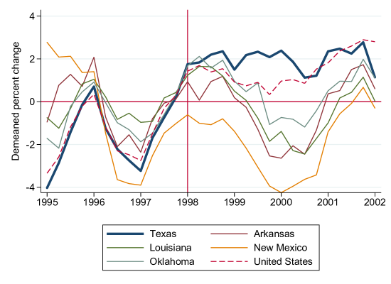
Figure 1: Annual Percent Change in Real House Prices (demeaned) in the United States, Texas, and Border States

Figure 1 plots the demeaned annual percent change in real house prices using raw data in Texas, the United States, and four states bordering Texas. The only time in this sample when Texas had greater real house price growth than either the full United States or its border states was for a few years after the law change in 1998.

5.2 Impact of HEL legalization on Texas house prices

This section presents the main results of this paper, the impact of HEL legalization on Texas house prices. Estimates are presented for four geographically nested samples and the data are weighted by the inverse of the number of zip codes in each state. The baseline specification contains year fixed effects, zip code fixed effects, a time trend interacted with an MSA dummy, and national log real oil prices interacted with an MSA dummy. The specification in the CBCP sample also includes contiguous border county pair by year fixed effects as in Dube et al. (2010). In the main analysis, robust standard errors are computed three ways: (1) clustered by state, (2) clustered by zip code, and (3) spatially correlated (Conley (1999)). This strategy is conservative in the border samples because there are relatively few clusters to precisely estimate standard errors clustered at the state level. All samples have enough zip codes to precisely estimate standard errors clustered at the zip code level. The largest standard error of the three is reported. Estimates from the baseline specification will be presented first, followed by an exploration of robustness.

Estimates from static regressions across the four samples (Table 2, columns 1–4) show that the HEL legalization raised Texas house prices $3.5\%-6.16\%$. All estimates are statistically significant at the $5\%$ level. The nested samples are progressively refined; column 1 uses the most aggregate sample (U.S.) whereas column 4 uses the most local sample (CBCP). Border samples help eliminate local time-varying differences to the extent that zip codes near each other are more likely affected by the same local shocks such as hurricanes and factory shutdowns. The effect was $3.5\%$ in the U.S. sample, $6.16\%$ in the Border State sample, $4.76\%$ in the Border sample, and $4.13\%$ in the CBCP sample. There is no systematic pattern in the size of the effect as the sample becomes more refined. The preferred estimate, ${\color[rgb]{.5,0,.5}\hat{\beta}_{DID}}=4.13\%$, is chosen from the CBCP sample because it is the most local sample with the most comprehensive battery of fixed effects.

Next, estimates from dynamic regressions (Table 2, columns 5–8) help rule out the biggest concern: upward pretrends. If Texas house prices were on an upward pretrend (relative to control zip codes) before the law change, that would raise concerns that some other factor was causing them to rise and that they would have continued to rise without the treatment.

The coefficients and 95% confidence intervals from the dynamic regressions for all four samples are plotted in Figure 2 and show a positive ${\color[rgb]{.5,0,.5}\hat{\eta}_{k}}>0$ and statistically significant effect after the law change. In the U.S. and CBCP samples, the effect was positive in 1998 but did not become statistically significant until 1999 in the U.S. sample and 2000 in the CBCP sample. The pretrends are parallel in all samples and show no evidence of anticipation before the law was implemented. Estimates in two of the samples, Border State and CBCP, have parallel pretrends only after including the oil price MSA interactions. The oil price MSA interaction is a valuable control because oil prices play an important economic role in Texas and its border states (Murphy et al. (2015)).

5.2.1 Robustness

This section investigates whether the main results in Table 2 are robust to (1) the method used for estimating standard errors, (2) the inclusion of covariates and an alternative specification of the outcome variable, (3) the restriction to border city samples, and (4) the method used to construct the house price index. Estimates in Table 8 explore whether the treatment effect remains significant when standard errors are conventional (OLS), robust (EHW), clustered by five-digit zip code, three-digit zip code, county FIPS code, MSA, state, or spatially correlated (SHAC). For the CBCP sample, standard errors are also clustered by county pair, double clustered by county pair and zip code, and double clustered by county pair and state. All estimates are statistically significant at least at the $5\%$ significance level. The only clear pattern is that the main treatment effect is significant at the $1\%$ level in all samples when standard errors are spatially correlated as in Conley (1999) or clustered at the three-digit zip code or smaller level. There does not seem to be an obvious pattern as standard errors are clustered at larger levels. In the U.S. and CBCP samples, the standard error falls as we move from MSA to state clusters, whereas the standard error estimates rise slightly in the Border State and Border samples.

Estimates in Table 3 investigate whether the treatment effect in Table 2 is robust to the inclusion of covariates including national interest rates interacted with state dummies, real income per capita, and population. The table also explores an alternative specification of the outcome variable using annual real house price growth (as opposed to log real house prices). The treatment effect remains positive and statistically significant across samples and specifications. In specifications using log real house prices as the outcome variable, including covariates slightly reduces the estimates in the U.S. and Border State samples and slightly raises the estimates in the Border and CBCP samples. In specifications using real house price growth as the outcome variable, the estimates are larger in the U.S. sample and smaller in the other three samples.

Estimates in Table 4 study the impact of HEL legalization on house prices in four border city samples. The advantage of these smaller samples is they can potentially provide better control for local unobserved heterogeneity. In addition, these estimates can help alleviate concerns about the indirect mechanism to the extent that border cities can be viewed as one economy. The samples are (1) Texarkana, the only MSA in Texas with zip codes in another state, (2) the Dallas-Fort Worth (DFW) Combined Statistical Area (CSA), which includes zip codes in Bryan County, Oklahoma, (3) the El Paso-Las Cruces CSA, which includes zip codes in Doña Ana County, New Mexico, and (4) the Texoma area, which includes counties in Oklahoma near Lake Texoma. The estimates in these border samples are between $3.75\%$ and $5.97\%$ and statistically significant.

Estimates in Table 9 investigate whether the treatment effect in Table 2 is robust to the method used for constructing the house price index. The outcome variables in this table are from the ZHVI, which is constructed differently from the FHFA index used in the main analysis. These estimates remain positive, statistically significant, and similar to the main estimates. Another advantage of the ZHVI index is that it can be directly interpreted as the median dollar house value in a zip code year. Table 9 also presents estimates of the HEL legalization on real ZHVI levels, finding an inflation-adjusted effect between $\$2,714.41$ and $\$5,363.34$.

5.2.2 Synthetic controls and placebo tests

This section investigates the impact of HEL legalization on Texas house prices using the synthetic control method (Abadie et al., 2010). Athey and Imbens (2017) called this “the most important innovation in the policy evaluation literature in the last 15 years. This method builds on difference-in-differences estimation, but uses systematically more attractive comparisons.” Cavallo et al. (2013) extend the method to allow for multiple units to experience treatment. This is useful because each Texas zip code received the treatment. Doudchenko and Imbens (2016) generalize the synthetic control method to allow nonconvex weights and a permanent additive difference between the treated and control units. They show that this powerful generalization nests many existing approaches as special cases including classical difference-in-differences and matching methods.

Let $Y_{z,t}$ denote the outcome variable for treated zip code $z$ in year $t$ and $Y_{j,t}$ the outcome for untreated zip code $j$. Let $Y_{z,pre}$ and $Y_{j,pre}$ be vectors of the outcome variables in the pretreatment years. Let $Y_{C,pre}$ be a matrix of predictors whose columns consist of $Y_{j,pre}$ (outcome variables for all control zip codes in the pretreatment years) as well as other control variables (national oil prices). The Doudchenko and Imbens (2016) estimator minimizes the distance between the treated outcome and an affine combination of the untreated outcome for the pretreatment period, regularized by the elastic-net (en) penalty (Zou and Hastie, 2005):

$$\left(\hat{\mu}^{en},\hat{\omega}^{en}\right) =\underset{\mu,\omega}{\operatorname*{argmin}}\text{ }\lVert Y_{z,pre}-\mu-Y_{C,pre}\cdot\omega\rVert_{2}^{2}+\lambda\cdot\left(\alpha\lVert\omega\rVert_{1}+(1-\alpha)\lVert\omega\rVert_{2}\right)$$

The parameter $\lambda$ determines the amount of regularization, and $\alpha$ determines the type. The case $\alpha=1$ corresponds to a LASSO penalty function, which captures a preference for parsimony via a small number of nonzero weights. The case $\alpha=0$ corresponds to a Ridge penalty function, which captures a preference for smaller weights. Doudchenko and Imbens (2016) propose a cross-validation procedure to select the regularization parameters $\lambda$ and $\alpha$ that minimize the average mean squared prediction error for all untreated units.

These estimates give the counterfactual outcome for treated zip code $z$ if it did not receive the treatment as a function of the control zip codes:

$$\hat{Y}_{z,t}(0) =\hat{\mu}^{en}+Y_{C,t}\hat{\omega}^{en},$$

where $Y_{C,t}$ is a row vector consisting of outcomes for the control zip codes and national oil prices in year $t$. The identifying assumption is that the relationship between the treated and control outcome variables, given by $\hat{\mu}^{en}$ and $\hat{\omega}^{en}$, would have remained the same in absence of the treatment. While this is defended in the same way as in Section 4.2, the advantage of the synthetic control estimator is a more attractive control group with tighter pretrends.

The estimated treatment effect for zip code $z$ is the gap (i.e., difference) between the observed and counterfactual outcome ${\color[rgb]{.5,0,.5}\hat{\eta}_{z,t}}=Y_{z,t}-\hat{Y}_{z,t}(0)$. The extension by Cavallo et al. (2013) allows for more than one zip code to experience treatment. Let $z\in\left\{1,\dots,Z\right\}$ be the index for all treated zip codes; then the average treatment effect in Texas (across all Texas zip codes) in year $t$ is given by ${\color[rgb]{.5,0,.5}\hat{\eta}_{TX,t}}=\frac{1}{Z}\sum_{z=1}^{Z}{\color[rgb]{.5,0,.5}\hat{\eta}_{z,t}}$. The average post-treatment effect is defined similarly ${\color[rgb]{.5,0,.5}\hat{\eta}_{TX}}=\frac{1}{\#\left\{t\geq 1998\right\}}\sum_{t\geq 1998}{\color[rgb]{.5,0,.5}\hat{\eta}_{TX,t}}$.

The synthetic control estimates using the Border State sample are presented in Figure 3. Panel A plots the treatment effect for each Texas zip code ${\color[rgb]{.5,0,.5}\hat{\eta}_{z,t}}$ in gray and the treatment effect averaged across all Texas zip codes ${\color[rgb]{.5,0,.5}\hat{\eta}_{TX,t}}$ in blue. Panel B plots the corresponding placebo estimates for each untreated zip code in gray as well as the average across untreated zip codes in blue.

Observe that before the treatment year, 1998, the treatment effect in both the Texas and control zip codes is approximately zero as intended. After 1998, the treatment effect in Texas zip codes is mostly positive, whereas the placebo treatment effects in control zip codes are equally positive and negative.

The treatment effect averaged over all post-treatment years in Texas is ${\color[rgb]{.5,0,.5}\hat{\eta}_{TX}}=4.58\%$. It is heartening to see that the average treatment effect across Texas zip codes is positive and of a similar magnitude as the estimates in the main analysis. The average post-treatment effect in the control group is ${\color[rgb]{.5,0,.5}\hat{\eta}_{C}}=-0.24\%$, indicating no evidence of a placebo effect.

5.3 Treatment effect heterogeneity

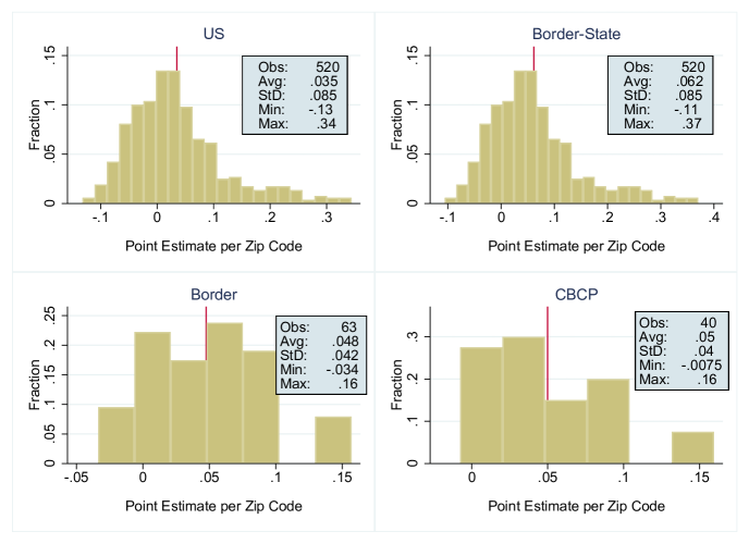
Figure 6: Impact of HEL Legalization on Texas House Prices, Heterogeneity Across Zip Codes

This section explores if and in what ways the effect differed across treated zip codes. Figure 6 presents histograms and summary statistics of the treatment effect for each treated zip code in the four geographically nested samples. These estimates are from regressions in the baseline specification (Table 2, columns 1–4), except the term $\text{Texas}\times\text{Post}$ is interacted with an indicator for each zip code. The histograms reveal that there is heterogeneity in the effect across zip codes.

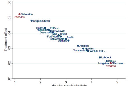
Figure 5: Impact of HEL Legalization on Texas House Prices by MSA Elasticity

Table 5 presents estimates from triple-difference regressions to investigate treatment effect heterogeneity along four dimensions: housing supply elasticity, income per capita, the unemployment rate, and median house price level. Estimates using the Saiz (2010) measure of supply elasticity (Table 5, column 1) show that zip codes in more elastic MSAs saw a smaller rise in prices. This is consistent with predictions from a partial equilibrium model; a rise in housing demand should have a bigger impact on prices in locations where it is relatively hard to build (Figure 4). The rise in house prices was $0.9\%$ lower per unit of elasticity. If housing supply was perfectly inelastic, the average treatment effect would be the intercept $6.3\%$. The fitted treatment effect is plotted against elasticity $\left(\hat{\text{ATE}}\left(H_{i}\right)={\color[rgb]{.5,0,.5}\hat{\beta}_{H,0}}+{\color[rgb]{.5,0,.5}\hat{\beta}_{H}}H_{i}\right)$ for each Texas MSA in Figure 5. The treatment effect varies considerably from $5.25\%$ in the most inelastic MSA (Galveston) to $2\%$ in the most elastic MSA (Sherman).

Table 5, column 2, investigates heterogeneity by prelaw log real income per capita. Zip codes in higher-income counties saw larger treatment effects. A 1% higher prelaw real income per capita corresponds to a $0.109\%$ larger treatment effect. Table 5, column 3, investigates heterogeneity by prelaw unemployment. Zip codes in counties with higher unemployment rates saw smaller treatment effects. A 1% higher prelaw unemployment rate corresponds to a $0.7\%$ smaller treatment effect.

Table 5, column 4, investigates heterogeneity by each zip code’s prelaw log real median house price level. Zillow estimated median house prices are used because the level of the FHFA index is not informative about median price levels. Ex ante pricier zip codes saw a bigger treatment effect. A 1% higher prelaw real median house price level corresponds to a $0.036\%$ larger treatment effect. The coefficient on $\text{Texas}\times\text{Post}$ is not interesting in this specification because there were no observations with zero house price levels.

These results complement Landvoigt et al. (2015). While Landvoigt et al. (2015) find that the credit expansion during the housing boom had a bigger impact on ex ante lower-priced homes in San Diego, this paper finds that the (exogenous) HEL legalization had a bigger impact on ex ante higher-priced homes in Texas. The credit expansion in Landvoigt et al. (2015) increased access to borrowers seeking all loans secured by housing; in particular purchase mortgages became available to many households that previously did not qualify. These previously purchase-constrained households tended to buy lower-priced homes. In contrast, the Texas law change did not affect access to purchase mortgages, but rather the ability of existing homeowners to extract equity by borrowing after they were already homeowners.

Together, the estimates in Table 5 (columns 2–4) provide evidence that households in more prosperous zip codes (with ex ante higher house price levels, higher income, and lower unemployment) value the option to pledge their home as collateral more strongly. There are several possible explanations. First, richer households typically enjoy a bigger tax shield on mortgage interest because (a) they have higher marginal tax rates and (b) they are more likely to itemize deductions. Second, these households tend to be more financially literate and are more likely to be aware of these equity extraction products (Lusardi and Mitchell, 2014). Third, rich households are more likely to qualify for these new loans as they tend to have better credit and more stable income (DeFusco and Mondragon, 2018).

To be clear, these results do not show that poorer households do not value HELs. The treatment effect was still positive (but smaller) in poorer zip codes. These results reveal that households expect to borrow more when they are not under distress (e.g., for education or entrepreneurship). These results highlight the asymmetric benefits of home equity borrowing due to mortgage underwriting requirements: households are less likely to qualify for HELs when they are experiencing economic distress.

5.4 Channels

This section investigates the mechanism behind the treatment effect on house prices by studying the impact of HEL legalization on various other outcome variables. The treatment effect could have occurred through two channels:

1. Direct Channel: the law caused a rise in demand for owner-occupied housing due to the new option allowing homes to be pledged as collateral.

2. Indirect Channel: the law affected other variables that affect house prices. For example, if the law increased investment enough to stimulate the local economy, this could have raised demand for housing, thus raising the price.

If variables known to affect house prices such as rent, population, income, and unemployment were not affected by the law change, that would provide evidence that the direct channel drove the treatment effect.

Estimates presented in Table 6 show that the law did not lead to economically or statistically significant changes in real rents, population, or real income per capita. The rent regressions are particularly informative as classical economic theory predicts that the price of housing should have been equal to the present discounted value of rents before the legalization of HELs: $p_{t}=\mathbb{E}_{t}\sum_{j=1}^{\infty}\frac{Rent_{t+j}}{(1+r_{t+1})\times\cdots\times(1+r_{t+j})}$. After the HEL legalization, the price should reflect both the housing service flow (rent) and the additional collateral service flow: $p_{t}=\mathbb{E}_{t}\sum_{j=1}^{\infty}\frac{Rent_{t+j}+{\color[rgb]{.5,0,.5}\textbf{CSF}_{\textbf{t+j}}}}{(1+r_{t+1})\times\cdots\times(1+r_{t+j})}$. The rent regression helps reassure us that the treatment effect is not due to indirect effects on rent. There was a small but statistically significant rise in the unemployment rate of $0.3\%$ (Table 6, column 4), but this works against the indirect channel as higher unemployment is associated with lower house price growth. In addition, Kumar and Liang (2019) find that Texas GDP was unaffected by this law change.

While the falsification tests address concerns about observed economic impact of the law change, estimates in border cities help control for unobserved economic impact to the extent that a border city (such as Texarkana) is one economy. Estimates in the border city samples (Table 4) are positive and statistically significant, providing additional support in favor of the direct channel.

Various other concerns regarding the mechanism behind the treatment effect are considered and addressed below:

1. Home Improvement Loans: if Texans used HELs to improve their homes, the rise in house prices might be due to the higher quality of the properties and not due to the demand for HELs.
   A: Home improvement loans were available before 1998 (Section 2).

2. Piggy-Back Loans: HELs could have increased purchase mortgage debt capacity for households that used second liens (“piggy-back mortgages”) to avoid mortgage insurance and obtain bigger loans (Lee et al., 2013).
   A: This was not a relevant factor in Texas because of the 80% LTV limit for all liens obtained after purchase.

Together, the falsification tests and border city estimates suggest that the law change did not have a significant impact on variables related to house prices, providing evidence that the treatment effect occurred mainly through the direct channel.

5.5 The marginal buyer

This section investigates whether the law change affected homeownership in Texas. The law change created a new benefit for homeownership: the option to extract equity without selling the home. Hence, if households value this option, and if house prices were held constant, demand for owner-occupied housing would be expected to rise. In equilibrium, the rise in demand should have raised house prices until the marginal buyer was indifferent between owning and renting. The same logic applies to potential owners deciding whether to live in Texas (or a nearby state).

Estimates presented in Table 6, columns 2 and 5–7, show the law did not lead to economically or statistically significant changes in population, MSA-level homeownership rates, household-level homeownership (using AHS survey data), or single-family building permits. In addition, Kumar (2018) finds no evidence of migration using IRS tax return data. These estimates provide evidence that the rise in house prices was sufficient to offset the rise in demand for ownership, keeping the marginal buyer indifferent between renting and owning.

5.6 External validity and discussion

This paper finds that after-purchase collateral service flows had a positive impact on the price of owner-occupied housing in Texas (over 500 treated zip codes) after 1998. The conceptual framework predicts that collateral service flows should have a positive impact on the prices of other assets, in other locations, at other times. In particular, the effect is likely higher for housing in other states, because Texas is the only state with an 80% limit on home equity extraction. More generally, collateral service flows for purchase loans are expected to have a positive effect on asset prices as well. Unfortunately, it is notoriously difficult to empirically identify the impact of purchase mortgage leverage on house prices due to simultaneity: on the one hand, a rise in purchase mortgage credit supply can raise housing demand and thus house prices; on the other hand, higher house prices require potential homebuyers to get bigger purchase mortgages.

There is little empirical work to compare the estimate to, because it is unusual to find a setting where it was illegal to pledge an asset as collateral after purchase. However, there is a growing literature in quantitative macroeconomics that seeks to understand whether households are liquidity-constrained and the role of illiquid housing wealth. In particular, Gorea and Midrigan (2018) observe that housing is an important component of wealth for American households and seek to quantify the extent to which housing wealth is illiquid. They study this question using a life-cycle model with uninsurable idiosyncratic risks in which they explicitly model key institutional details including LTV constraints, payment-to-income (PTI) constraints, long-term amortizing mortgages, and transaction costs of refinancing. Their model predicts that three-quarters of homeowners are liquidity-constrained, in that they would be better off if they could convert housing equity into liquid wealth. These homeowners are willing to pay five cents, on average, for every additional dollar of liquidity extracted from their homes. Liquidity constraints increase the average marginal propensity to consume out of a transitory income windfall by about 40%. Their model predicts that frictions that prevent homeowners from tapping home equity are sizable.

Gorea and Midrigan (2018) proceed to simulate the Texas HEL legalization in their model. They find that the addition of the option to extract home equity raises equilibrium house prices 5.5%. This is within the range of the main estimates (Table 2, columns 1–4) and slightly higher than the preferred estimate in the CBCP sample of 4.13%. This can be explained because in their model housing is in fixed supply, hence perfectly inelastic. Interestingly, they find that the addition of the option to extract home equity causes a small drop in the homeownership rate from 66% to 64%, whereas this paper finds a statistically insignificant rise of 0.3% (Table 6).

6 Conclusion

A large body of literature studies the impact of credit constraints on borrowing, consumption, and investment. This paper finds that there is also an impact on the prices of assets that can be pledged as collateral. Estimates using zip code data show that the HEL legalization raised Texas house prices 4.13%. If households fear they will be credit-constrained, they should value assets that facilitate their future ability to borrow. Hence, the treatment effect estimated in this paper can be interpreted as price-based evidence that households are credit-constrained and value HELs to facilitate future consumption smoothing.

Prices rose more in locations with inelastic housing supply, higher prelaw income, lower unemployment, and higher house price levels. This reveals that richer households value the option to pledge their home as collateral more strongly. This heterogeneity can be explained by (1) the greater tax shield available to rich households, (2) the tendency of rich households to be more financially literate and aware of these financial products, and (3) the tendency of rich households to be more likely to qualify for HELs as they tend to have better credit and more stable income. The law change did not affect variables known to be related to house prices such as rent, population, and income. There was a small but statistically significant rise in the unemployment rate, which works against the indirect channel. Moreover, the border and border city samples, which help control for local unobserved heterogeneity, provide further evidence that the effect was direct. These results indicate that the treatment effect was mainly driven by the direct channel. Finally, the law change did not affect Texas population, homeownership, or building permits. This offers evidence that the rise in house prices was sufficient to keep the marginal homebuyer indifferent between owning and renting.

There are several avenues for future work. It would be interesting to estimate how collateral service flows affect the price of other assets such as stocks and Treasury bonds. Between 1934 and 1974, the Federal Reserve changed the initial margin requirement (regulation T) for the U.S. stock market 22 times (Jylhä, 2018). A good experiment would compare the same stock (possibly traded on different exchanges) but where certain shares of the stock are not affected by the margin requirements. It would also be interesting to disentangle the components of collateral service flows. Loans secured by housing have two benefits: a lower interest rate and a higher debt capacity. It would be helpful to separately identify the fraction of collateral service flow that is due to interest rate savings compared to debt capacity.

In conclusion, owner-occupied housing comes with a valuable option to pledge the home as collateral in the future. The legalization of HELs in Texas provides evidence that house prices reflect this.

Appendix A Appendix A. Figures

A.1 Percent Change in Real House Prices

This figure plots the annual demeaned percent change in real house prices in the United States, Texas, and its four border states. There is a vertical red line in 1998, the year home equity loans were legalized in Texas. The house price data are from the FHFA AT Index. House prices are deflated by the CPI-U, as explained in the paper. Data sources can be found in Table 7.

A.2 Pretrends

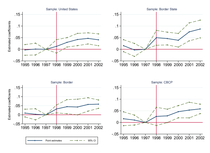
Figure 2: Impact of HEL Legalization on Texas House Prices in Four Geographically Nested Samples

This figure plots point estimates ${\color[rgb]{.5,0,.5}\hat{\eta}_{k}}$ and 95% confidence intervals from the dynamic regression in Table 2. There is a vertical red line in 1998, the year of the law change. Data sources can be found in Table 7.

A.3 Synthetic Controls

Figure 3: Impact of HEL Legalization on Texas House Prices Using Synthetic Controls

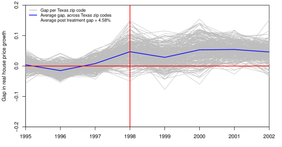
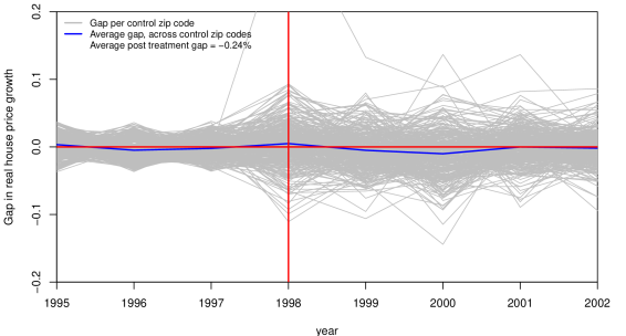
Panel A: Zip Codes in Texas Panel B: Zip Codes in Border States Panel A presents the gap (treatment effect) in real house price growth for each treated zip code ${\color[rgb]{.5,0,.5}\hat{\eta}_{z,t}}$ (gray) estimated using a synthetic control sample consisting of zip codes in border states, as explained in Section 5.2.2. The blue curve is the average gap across all treated zip codes each year ${\color[rgb]{.5,0,.5}\hat{\eta}_{TX,t}}$. The average post-treatment effect in Texas is ${\color[rgb]{.5,0,.5}\hat{\eta}_{TX}}=4.58\%$. Panel B presents the corresponding placebo gaps for zip codes in border states that did not receive the treatment. The average post-treatment effect in the control group is ${\color[rgb]{.5,0,.5}\hat{\eta}_{\text{C}}}=-0.24\%$. There is a vertical red line in 1998, the year of the law change. Data sources can be found in Table 7.

A.4 Supply Elasticity Theory

This figure compares the impact of a rise in housing demand on house prices in two cities with different supply elasticities. Price (P) is on the vertical axis, and quantity (Q) is on the horizontal axis. Initially, the price of housing is the same in both cities. A rise in demand causes prices to rise more in the relatively inelastic city. This figure is from a discussion by Loretta Mester at the Federal Reserve Bank of Philadelphia.

A.5 Elasticity Fitted Values

This figure plots the fitted average treatment effect $\left(\hat{\text{ATE}}\left(H_{i}\right)={\color[rgb]{.5,0,.5}\hat{\beta}_{H,0}}+{\color[rgb]{.5,0,.5}\hat{\beta}_{H}}H_{i}\right)$ for each MSA against housing supply elasticity. The estimates are from triple-difference regressions presented in Table 5. This figure includes all 21 Texas MSAs. Galveston, the most inelastic MSA, had a 5.25% effect, whereas Sherman, the most elastic MSA, had a 2% effect. The measure of housing supply elasticity is from Saiz (2010). Data sources can be found in Table 7.

Appendix B Appendix B. Tables

B.1 Summary Statistics

Table 1: Summary Statistics

Sample:	Pre-1998			Post-1998
Variables	Texas	Control	Difference	Texas	Control	Difference
LTV (%)	83.17	79.29	3.88*	77.57	81.52	–3.95***
	(1.46)	(0.73)	(1.50)	(0.99)	(0.49)	(0.40)
Interest Rate (%)	7.58	7.58	0.00	6.80	6.77	0.03
	(0.17)	(0.08)	(0.16)	(0.28)	(0.14)	(0.04)
Real House Price ($000)	82.01	74.96	7.05	92.78	81.08	11.70*
	(3.83)	(1.91)	(4.73)	(3.17)	(1.58)	(4.71)
Real Rent ($)	482.67	488.56	–5.88	502.77	502.96	–0.19
	(5.16)	(1.38)	(22.78)	(4.56)	(1.22)	(20.65)
Population Growth (%)	1.74	1.08	0.66**	1.62	0.93	0.68***
	(0.07)	(0.07)	(0.22)	(0.09)	(0.08)	(0.09)
Real Income Per Cap ($)	12,585.55	11,885.64	699.91**	14,115.58	13,312.92	802.66***
	(93.08)	(86.11)	(159.86)	(105.47)	(97.57)	(113.15)
Unemployment Rate (%)	6.30	6.38	–0.08	5.41	5.22	0.19
	(0.12)	(0.11)	(0.60)	(0.07)	(0.07)	(0.41)
Homeownership Rate (%)	56.96	60.88	–3.91	60.80	64.52	–3.72*
	(0.80)	(0.90)	(2.92)	(0.71)	(0.79)	(1.43)
Single-Family Permits	798.46	313.24	485.22***	1,304.91	400.52	904.39***
	(55.69)	(52.80)	(42.80)	(88.26)	(83.68)	(53.88)
Saiz Supply Elasticity	3.06	3.60	–0.54	3.06	3.60	–0.54
	(0.43)	(0.47)	(0.36)	(0.43)	(0.47)	(0.36)

This table presents summary statistics for the treatment group (Texas) and control group (border states) six years before and after the law change. The standard deviation of each variable is in parentheses below the average. Tests for differences between treatment and control groups using robust standard errors as described in the paper are also reported. Nominal variables are adjusted for inflation, as explained in Section 4. Supply elasticity, as estimated by Saiz (2010), does not vary over time in the sample. Data sources can be found in Table 7. * p$<$.1; ** p$<$.05; *** p$<$.01.

B.2 Main

Table 2: Impact of HEL Legalization on Texas House Prices

	(1)	(2)	(3)	(4)	(5)	(6)	(7)	(8)
Variables	United States	Border State	Border	CBCP	United States	Border State	Border	CBCP
TexasPost	0.0350***	0.0616**	0.0476**	0.0413***
	(0.0099)	(0.0221)	(0.0151)	(0.0126)
Texas95					-0.0027	0.0155	0.0096	0.0159
					(0.0117)	(0.0131)	(0.0108)	(0.0107)
Texas96					0.0009	-0.0029	0.0027	0.0101
					(0.0129)	(0.0142)	(0.0110)	(0.0085)
Texas98					0.0126	0.0498***	0.0322**	0.0260
					(0.0147)	(0.0163)	(0.0111)	(0.0166)
Texas99					0.0298***	0.0462***	0.0448**	0.0283*
					(0.0103)	(0.0110)	(0.0140)	(0.0146)
Texas00					0.0421***	0.0388**	0.0429*	0.0462***
					(0.0134)	(0.0136)	(0.0155)	(0.0128)
Texas01					0.0468***	0.0749***	0.0571**	0.0533**
					(0.0122)	(0.0139)	(0.0133)	(0.0127)
Texas02					0.0407***	0.0871***	0.0587***	0.0583***
					(0.0130)	(0.0143)	(0.0117)	(0.0104)
$N$	143,637	11,310	1,365	2,041	143,637	11,310	1,365	2,041
$R^{2}$	0.9771	0.9825	0.9814	0.9848	0.9772	0.9833	0.9820	0.9847

This table reports estimates of the effect of a law change (which legalized HELs in Texas) on house prices in geographically nested samples. Each column reports a separate regression estimated at the zip code year level where the dependent variable is the log of the real house price index. In columns 1–4, coefficients are reported for the interaction of the Texas dummy with an indicator for whether the year of observation falls on or after 1998. In columns 5–8, coefficients are reported for interactions of the Texas dummy with year indicators. All specifications include zip code and year fixed effects, state time trends, and national oil prices interacted with MSA dummies. Specifications using the CBCP sample also include contiguous border county pair by year fixed effects. Standard errors, computed using methods described in Section 5.2, are reported in parentheses. Data sources can be found in Table 7. * p$<$.1; ** p$<$.05; *** p$<$.01.

B.3 Specification Robustness

Table 3: Impact of HEL Legalization on Texas House Prices, Specification Robustness

(1) (2) (3) (4) Variables United States Border State Border CBCP A. Outcome: Log real house price index Baseline 0.0350*** 0.0616** 0.0476** 0.0413*** (0.0099) (0.0221) (0.0151) (0.0126) Covariates 0.0330*** 0.0558** 0.0480** 0.0499*** (0.0086) (0.0196) (0.0166) (0.0159) $N$ 143,637 11,310 1,365 2,041 B. Outcome: Real house price growth Baseline 0.0389*** 0.0563*** 0.0317** 0.0409*** (0.0071) (0.0079) (0.0110) (0.0124) Covariates 0.0374*** 0.0539*** 0.0288** 0.0375*** (0.0055) (0.0065) (0.0100) (0.0125) $N$ 141,986 11,185 1,347 1,808

This table reports estimates of the effect of a law change (which legalized HELs in Texas) on house prices in geographically nested samples. Each entry reports a separate regression estimated at the zip code year level where the dependent variable is the log of the real house price index in panel A or real house price growth in panel B. All specifications include zip code and year fixed effects, state time trends, and national oil prices interacted with MSA dummies. Specifications using the CBCP sample also include contiguous border county pair by year fixed effects. Specifications in rows labeled “Covariates” include U.S. interest rates interacted with state dummies, real income per capita, and population. Standard errors, computed using the methods described in Section 5.2, are reported in parentheses. Data sources can be found in Table 7. * p$<$.1; ** p$<$.05; *** p$<$.01.

B.4 Border City Samples

Table 4: Impact of HEL Legalization on Texas House Prices in Border City Samples

	(1)	(2)	(3)	(4)
Variables	Texarkana	DFWBorder	ElPasoLasCruces	Texoma
Treated_post1998	0.0588**	0.0405**	0.0597***	0.0375**
	(0.0091)	(0.0131)	(0.0133)	(0.0126)
N	39	65	195	78
$R^{2}$	0.961	0.994	0.996	0.992

This table reports estimates of the effect of a law change (which legalized HELs in Texas) on house prices in various border city samples. Column 1 uses data from the Texarkana MSA, column 2 uses data from the Dallas-Fort Worth (DFW) CSA, column 3 uses data from the El Paso Las Cruces CSA, and column 4 uses data from the Texoma area. Each column reports a separate regression estimated at the zip code year level where the dependent variable is the log of the real house price index. In columns 1–4, coefficients are reported for the interaction of the Texas dummy with an indicator for whether the year of observation falls on or after 1998. All specifications include zip code and year fixed effects, state time trends, and national oil prices interacted with MSA dummies. Specifications using the CBCP sample also include contiguous border county pair by year fixed effects. Standard errors are reported in parentheses. Data sources can be found in Table 7. * p$<$.1; ** p$<$.05; *** p$<$.01.

B.5 Treatment Effect Heterogeneity

Table 5: Impact of HEL Legalization on Texas House Prices, Treatment Effect Heterogeneity

	(1)	(2)	(3)	(4)
Variables
$\text{Texas}\times\text{Post}$	0.063***	-1.002***	0.080***	-0.367***
	(0.011)	(0.246)	(0.015)	(0.122)
$\text{Texas}\times\text{Post}\times\text{Elasticity}$	-0.009**
	(0.004)
$\text{Texas}\times\text{Post}\times\text{LogRealIncomePre}$		0.109***
		(0.026)
$\text{Texas}\times\text{Post}\times\text{UnemploymentRatePre}$			-0.007***
			(0.002)
$\text{Texas}\times\text{Post}\times\text{LogRealMedianHousePricesPre}$				0.036***
				(0.011)
N	111,748	142,077	143,676	132,431
$R^{2}$	0.651	0.616	0.611	0.626
Max $H_{i}$	4.749	9.949	19.95	13.77
Min $H_{i}$	1.18	8.936	1.95	10.16
TE Max $H_{i}$	.0201	.0803	-.0619	.131
TE Min $H_{i}$	.0525	-.03	.066	.000534

This table reports estimates of the effect of a law change (which legalized HELs in Texas) on house prices. Each column reports a separate regression in which the treatment effect is allowed to vary based on four measures of heterogeneity: supply elasticity, prelaw log real income per capita, unemployment, and log real median house prices. Prelaw variables are set equal to their average before 1998. The dependent variable is the log of the real house price index. The first row reports coefficients for the interaction of the Texas dummy with an indicator for whether the year of observation falls on or after 1998. This represents the treatment effect if the measure of heterogeneity is equal to zero. The remaining rows report the coefficient on the triple interaction between the Texas dummy, an indicator for the treatment period, and one of four measures of heterogeneity. All specifications include zip code and year fixed effects, state time trends, and national oil prices interacted with MSA dummies. Specifications using the CBCP sample also include contiguous border county pair by year fixed effects. Standard errors are clustered at the state level and are reported in parentheses. When interpreting the parameters in this table, take into account that some measures of heterogeneity are in logs while others are not. Data sources can be found in Table 7. * p$<$.1; ** p$<$.05; *** p$<$.01.

B.6 Other Outcome Variables: Falsification, Channels, Marginal Buyer

Table 6: Impact of HEL Legalization on Other Outcome Variables

	(1)	(2)	(3)	(4)	(5)	(6)	(7)
			Log		Home	Home	Log
	Log	Log	Real Income	Unemployment	Ownership	Owner	Single Family
Variables	Real Rent	Population	Per Capita	Rate	Rate	AHS	Permits
$\text{Texas}\times\text{Post}$	0.003	0.000	-0.001	0.003**	0.003	0.004	0.048
	(0.005)	(0.007)	(0.005)	(0.001)	(0.004)	(0.004)	(0.033)
N	16,276	40,690	40,404	21,606	947	171,966	36,614
$R^{2}$	0.303	0.254	0.634	0.391	0.442	0.036	0.063

This table reports estimates of the effect of a law change (which legalized HELs in Texas) on six outcome variables: Log Real Rent, Log Population, Log Real Income Per Capita, the Unemployment Rate, the Homeownership Rate, and Log Single-Family Building Permits. Coefficients are reported for the interaction of the Texas dummy with an indicator for whether the year of observation falls on or after 1998. All specifications include year fixed effects along with location fixed effects at the most local level possible. Standard errors are clustered at the state level and are reported in parentheses. Data sources can be found in Table 7. * p$<$.1; ** p$<$.05; *** p$<$.01.

Appendix C For Online Publication: Online Appendix Figures

C.1 Treatment Effect Heterogeneity by Zip Code

Note. This figure presents histograms and summary statistics of the treatment effect for each zip code in the geographically nested samples. There is a vertical red line at the mean. Data sources can be found in Table 7.

Appendix D For Online Publication: Online Appendix Tables

D.1 Datasets

Table 7: Datasets

Variable	Level	Source	# Locations	TX
House Price Index	5-digit zip code	FHFA	17,936 zips	918 zips
House Price Index	state	FHFA	51: US & DC	1
LTV (1st purchase lien)	state	FHFA	51: US & DC	1
Interest Rate	state	FHFA	51: US & DC	1
Median House Prices	5-digit zip code	Zillow	$12.665$ zips	$576$ zips
Median Rent (historic)	MSA	Zillow	$313$ MSAs	$21$ MSAs
Supply Elasticity	MSA	Saiz (2010)	269 MSAs	21 MSAs
Employment	county	BLS	2,581 fips	153 fips
Income	county	BEA	2,581 fips	153 fips
Population	county	Census	2,581 fips	153 fips
Building permits	county	Census	3,072 fips	229 fips
Homeownership Rate	MSA	Census	75 MSAs	5 MSAs
Homeownership	Household Survey	AHS	123 MSAs	9 MSAs
Oil Prices	US	EIA	-	-
10 year Treasury	US	Treasury	-	-
Inflation Expectations	US	Livingston survey	-	-
CPI-U	US	BLS	-	-

Note. This table lists sources for the different variables used in this paper. All data are annual except for the FHFA state house price index, Zillow rent index, and the Zillow Home Value Index. The Metropolitan Statistical Areas (MSAs) are defined by the United States Office of Management and Budget. The Federal Information Processing Standards (fips) codes uniquely identify counties. The AHS survey data is at the household level, but the most local geographic level available is the MSA.

D.2 Standard Error Robustness

Table 8: Impact of HEL Legalization on Texas House Prices, Standard Error Robustness

	(1)	(2)	(3)	(4)
METHOD	US	Border-State	Border	CBCP
TexasPost	0.0350	0.0616	0.0476	0.0413
OLS	(0.0049)***	(0.0045)***	(0.0098)***	(0.0116)***
EHW	(0.0029)***	(0.0037)***	(0.0087)***	(0.0127)***
Zip5	(0.0030)***	(0.0045)***	(0.0097)***	(0.0115)***
Zip3	(0.0129)***	(0.0164)***	(0.0148)***	(0.0120)***
Fips	(0.0149)**	(0.0179)***	(0.0143)***	(0.0120)***
Msa	(0.0167)**	(0.0210)***	(0.0139)***	(0.0116)***
State	(0.0075)***	(0.0221)**	(0.0151)**	(0.0039)***
SHAC	(0.0099)***	(0.0121)***	(0.0098)***	(0.0111)***
Pair				(0.0128)***
Pair Zip5				(0.0126)***
Pair State				(0.0083)***
$N$	143,637	11,310	1,365	2,041
$R^{2}$	0.9772	0.9826	0.9817	0.9851

Note. This table repeats the estimates in Table 2: columns 1-4, using a variety of different methods to estimate standard errors. Each column corresponds to the sample and each row (after the first) corresponds to the method for estimating standard errors. All specifications include zip code and year fixed effects, state time trends, and national oil prices interacted with MSA dummies. Specifications using the CBCP sample also include contiguous border county pair by year fixed effects. Data sources can be found in Table 7. * p$<$.1; ** p$<$.05; *** p$<$.01.

D.3 House Price Index Robustness

Table 9: Impact of HEL Legalization on Texas House Prices, House Price Index Robustness

	(1)	(2)	(3)	(4)	(5)	(6)	(7)	(8)
SAMPLES	US	US	Border-State	Border-State	Border	Border	CBCP	CBCP
VARIABLES	(lnY)	($Y)	(lnY)	($Y)	(lnY)	($Y)	(lnY)	($Y)
$\text{Texas}\times\text{Post}$	0.046***	5,363.34***	0.031***	2,714.41***	0.042***	4,020.57***	0.050***	3,027.09***
	(0.008)	(971.54)	(0.003)	(136.47)	(0.002)	(100.10)	(0.007)	(380.86)
N	1,277,495	1,277,495	126,806	126,806	14,662	14,662	14,948	14,948
$R^{2}$	0.992	0.973	0.995	0.996	0.994	0.996	0.994	0.995

Note. This table repeats the estimates in Table 2: columns 1-4, using data from Zillow. Each sample estimates the treatment effect two ways: using the log house real price index and using the real ZHVI (Zillow’s measure of median home value in a zip-code). All specifications include zip code and year fixed effects, state time trends, and national oil prices interacted with MSA dummies. Specifications using the CBCP sample also include contiguous border county pair by year fixed effects. Data sources can be found in Table 7. * p$<$.1; ** p$<$.05; *** p$<$.01.

Appendix E For Online Publication: Texas Legal Timeline

This appendix provides a brief timeline of relevant laws regarding home equity borrowing in Texas.

• Article XVI, Section 50 of Texas Constitution of 1876 protects homesteads from foreclosure for failure to pay all debts except the purchase loan, property taxes, or a mechanic’s lien.

• This section has only been amended twice before 1997; the first amendment extended protections to single adults in 1973 and the second amendment of 1995 related to divorce proceedings.

• December 1994, Texas Senate Interim Committee on Home Equity Lending comes out in strong support of easing restrictions on lending with limits on home equity lending to protect consumers, and called for the amendment proposal to be put on the ballot for voters to decide. The proposal did not gather the two-thirds majority in the House of Representatives, but it did pass the Senate, which was a first for such a proposal. The committee’s report was incorporated into House Joint Resolution 31 which passed the Texas House and Senate in May 1997.

• Voters approved Proposition 8 on 11-4-1997 with almost 60% voting yes of the 1.17 million votes cast, begins 1-1-1998, legalized Home Equity Loans without restrictions on how the money could be used, however the total value of all liens on the home cannot exceed 80% of the fair market value. Reverse mortgages and cash-out refinance loans were also legalized.

• Several problems with Proposition 8 in the first year.
  HELs not allowed for those who live on more than one acre of land.
  Reverse mortgage rules made the loans ineligible for purchase by Fannie Mae.

• Proposition 2 on the November 2, 1999 ballot corrected the shortcomings.
  Article XVI, Section 50 was amended to clear up the issues with reverse mortgages.
  Article XVI, Section 51 was amended by increasing the acreage limit used to define urban households to 10 acres.

Appendix F For Online Publication: Household’s Problem

This appendix solves the household’s problem presented in Section 3.

$$\max\text{ }\mathbb{E}_{0}\sum_{t=0}^{\infty}\beta^{t}u(c_{t},h_{t})$$

s.t.

$$c_{t}+p_{t}h_{t+1}+a_{t+1} \leq y_{t}+p_{t}h_{t}(1-\delta_{t})+(1+r_{t})a_{t} \lambda_{t}$$ (DBC )

$$-a_{t+1} \leq\kappa_{t}p_{t}h_{t} \mu_{t}$$ (CC )

Savings: $a_{t+1}$ at time $t$. If $a_{t+1}>0$, save, if $a_{t+1}<0$, borrow.
The multiplier on the dynamic budget constraint (DBC): $\lambda(s^{t})\beta^{t}\pi(s^{t})>0$
The multiplier on the collateral constraint (CC): $\mu(s^{t})\beta^{t}\pi(s^{t})\geq 0$
Complementary slackness: $\mu(s^{t})\beta^{t}\pi(s^{t})\left[\kappa(s^{t})p(s^{t})h_{t}(s^{t-1})+a_{t+1}(s^{t})\right]=0$

State variables in $s^{t}$: $y(s^{t})$, $h_{t}(s^{t-1})$, $a_{t}(s^{t-1})$, $r_{t}(s^{t-1})$, $\delta(s^{t})$, $\kappa(s^{t})$.
Choice variables in $s^{t}$: $c(s^{t})$, $h_{t+1}(s^{t})$, $a_{t+1}(s^{t})$.

$$\mathcal{L}=\sum_{t=0}^{\infty}\underset{s^{t}\in S^{t}}{\sum} \beta^{t}\pi(s^{t})u(c(s^{t}),h(s^{t}))$$

$$+ \lambda(s^{t})\beta^{t}\pi(s^{t})\left[y(s^{t})+p(s^{t})h_{t}(s^{t-1})(1-\delta(s^{t}))+\left(1+r_{t}(s^{t-1})\right)a_{t}(s^{t-1})\right]$$

$$- \lambda(s^{t})\beta^{t}\pi(s^{t})\left[c(s^{t})+p(s^{t})h_{t+1}(s^{t})+a_{t+1}(s^{t})\right]$$

$$+ \mu(s^{t})\beta^{t}\pi(s^{t})\left[\kappa(s^{t})p(s^{t})h_{t}(s^{t-1})+a_{t+1}(s^{t})\right]$$

In $s^{t}$ we have: $y(s^{t})$, $h_{t}(s^{t-1})$, $a_{t}(s^{t-1})$, $\delta(s^{t})$, $\kappa(s^{t})$.
In $s^{t}$ we choose: $c(s^{t})$, $h_{t+1}(s^{t})$, $a_{t+1}(s^{t})$. (Any two will pin down the third.)

$$\mathcal{L}_{c(s^{t})} =\beta^{t}\pi(s^{t})u_{1}(s^{t})+\lambda(s^{t})\beta^{t}\pi(s^{t})\left[-1\right]$$

$$=0$$

$$\Leftrightarrow$$

$$\lambda(s^{t}) =u_{1}(s^{t})$$

$$\mathcal{L}_{h_{t+1}(s^{t})} =\sum_{s^{t+1}|s^{t}}\beta^{t+1}\pi(s^{t+1})u_{2}(s^{t+1})$$

$$+\lambda(s^{t})\beta^{t}\pi(s^{t})\left[-p(s^{t})\right]$$

$$+\sum_{s^{t+1}|s^{t}}\lambda(s^{t+1})\beta^{t+1}\pi(s^{t+1})\left[p(s^{t+1})(1-\delta(s^{t+1}))\right]$$

$$+\sum_{s^{t+1}|s^{t}}\mu(s^{t+1})\beta^{t+1}\pi(s^{t+1})\left[\kappa(s^{t+1})p(s^{t+1})\right]$$

$$=0$$

$$\mathcal{L}_{a_{t+1}(s^{t})} =\lambda(s^{t})\beta^{t}\pi(s^{t})\left[-1\right]$$

$$+\mu(s^{t})\beta^{t}\pi(s^{t})\left[1\right]$$

$$+\sum_{s^{t+1}|s^{t}}\lambda(s^{t+1})\beta^{t+1}\pi(s^{t+1})\left(1+r_{t+1}(s^{t})\right)$$

$$=0$$

$$\Leftrightarrow$$

$$\lambda(s^{t})\beta^{t}\pi(s^{t}) =\mu(s^{t})\beta^{t}\pi(s^{t})+\sum_{s^{t+1}|s^{t}}\lambda(s^{t+1})\beta^{t+1}\pi(s^{t+1})\left(1+r_{t+1}(s^{t})\right)$$

$$\Leftrightarrow$$

$$\lambda(s^{t}) =\mu(s^{t})+\beta\left(1+r_{t+1}(s^{t})\right)\mathbb{E}_{t}[\lambda(s^{t+1})]$$

$$\text{recall }\lambda(s^{t}) =u_{1}(s^{t})\text{ (consumption foc)}$$

$$\Leftrightarrow$$

$$u_{1}(s^{t}) =\mu(s^{t})+\beta\left(1+r_{t+1}(s^{t})\right)\mathbb{E}_{t}[u_{1}(s^{t+1})]$$

This is the famous liquidity-constrained Euler equation! If the collateral constraint is not binding ($\mu=0$) or doesn’t exist, then this collapses to the usual frictionless Euler equation.

Using $\lambda(s^{t})=u_{1}(s^{t})$, we combine the consumption and housing FOCs.

$$u_{1}(s^{t})\beta^{t}\pi(s^{t})\left[p(s^{t})\right] =\sum_{s^{t+1}|s^{t}}\beta^{t+1}\pi(s^{t+1})u_{2}(s^{t+1})$$

$$+\sum_{s^{t+1}|s^{t}}u_{1}(s^{t+1})\beta^{t+1}\pi(s^{t+1})\left[p(s^{t+1})(1-\delta(s^{t+1}))\right]$$

$$+\sum_{s^{t+1}|s^{t}}\mu(s^{t+1})\beta^{t+1}\pi(s^{t+1})\left[p(s^{t+1})\kappa(s^{t+1})\right]$$

$$u_{1}(s^{t})\left[p(s^{t})\right] =\mathbb{E}_{t}\beta u_{2}(s^{t+1})$$

$$+\mathbb{E}_{t}u_{1}(s^{t+1})\beta\left[p(s^{t+1})(1-\delta(s^{t+1}))\right]$$

$$+\mathbb{E}_{t}\mu(s^{t+1})\beta\left[p(s^{t+1})\kappa(s^{t+1})\right]$$

$$p(s^{t}) =\mathbb{E}_{t}\beta\frac{u_{2}(s^{t+1})}{u_{1}(s^{t})}$$

$$+\mathbb{E}_{t}\beta\frac{u_{1}(s^{t+1})}{u_{1}(s^{t})}\left[p(s^{t+1})(1-\delta(s^{t+1}))\right]$$

$$+\mathbb{E}_{t}\beta\frac{\mu(s^{t+1})}{u_{1}(s^{t})}\left[p(s^{t+1})\kappa(s^{t+1})\right]$$

$$p(s^{t}) =\mathbb{E}_{t}\beta\frac{u_{1}(s^{t+1})}{u_{1}(s^{t})}\frac{u_{2}(s^{t+1})}{u_{1}(s^{t+1})}$$

$$+\mathbb{E}_{t}\beta\frac{u_{1}(s^{t+1})}{u_{1}(s^{t})}\left[p(s^{t+1})(1-\delta(s^{t+1}))\right]+\mathbb{E}_{t}\beta\frac{u_{1}(s^{t+1})}{u_{1}(s^{t})}\frac{\mu(s^{t+1})}{u_{1}(s^{t+1})}\left[p(s^{t+1})\kappa(s^{t+1})\right]$$

$$p(s^{t}) =\mathbb{E}_{t}\left[\beta\frac{u_{1}(s^{t+1})}{u_{1}(s^{t})}\left(\frac{u_{2}(s^{t+1})}{u_{1}(s^{t+1})}+\left[p(s^{t+1})(1-\delta(s^{t+1}))\right]+\frac{\mu(s^{t+1})}{u_{1}(s^{t+1})}\left[p(s^{t+1})\kappa(s^{t+1})\right]\right)\right]$$

$$\underbrace{p_{t}}_{\text{price}} =\mathbb{E}_{t}\left[\underbrace{\beta\frac{u_{1}(t+1)}{u_{1}(t)}}_{sdf}\times\left(\underbrace{\frac{u_{2}(t+1)}{u_{1}(t+1)}}_{\text{housing service flow}}+\underbrace{\frac{\mu(t+1)}{u_{1}(t+1)}\kappa_{t+1}p_{t+1}}_{\text{collateral service flow}}+\underbrace{(1-\delta_{t+1})p_{t+1}}_{\text{resale price}}\right)\right]$$

$$p_{t} =\mathbb{E}_{t}[M_{t+1}\times\left(s_{t+1}+CSF_{t+1}+(1-\delta_{t+1})p_{t+1}\right)]$$

We can use the equilibrium value of the multiplier:
$\mu(t+1)=u_{1}(t+1)-\beta\left(1+r_{t+2}(s^{t+1})\right)\mathbb{E}_{t+1}[u_{1}(t+2)]$

$$\mu_{t} =u_{c}(t)-\beta\left(1+r_{t+1}\right)\mathbb{E}_{t}[u_{c}(t+1)]$$

If there is no collateral constraint or the collateral constraint never binds ($\mu(s^{t})=0$), then housing has no collateral value ($CSF_{t}=0$).

F.1 Price Decomposition

Define $M_{t,j}\equiv M_{t}\times M_{t+1}\cdots M_{j-1}\times M_{j}$
Define the total dividend $d_{t}\equiv s_{t}+CSF_{t}$

$$p_{t} =\mathbb{E}_{t}\left[M_{t+1}\times\left(d_{t+1}+(1-\delta)p_{t+1}\right)\right]$$

$$=\mathbb{E}_{t}\left[M_{t+1}\times\left(d_{t+1}\right)\right]+(1-\delta)\mathbb{E}_{t}\left[M_{t+1}\times p_{t+1}\right]$$

$$=\mathbb{E}_{t}\left[M_{t+1}\times\left(d_{t+1}\right)\right]+(1-\delta)\mathbb{E}_{t}\left[M_{t+1}\times\mathbb{E}_{t+1}\left[M_{t+2}\times\left(d_{t+2}+(1-\delta)p_{t+2}\right)\right]\right]$$

$$=\mathbb{E}_{t}\left[M_{t+1}\times\left(d_{t+1}\right)\right]+(1-\delta)\mathbb{E}_{t}\left[M_{t+1}\times M_{t+2}\times\left(d_{t+2}+(1-\delta)p_{t+2}\right)\right]$$

$$=\mathbb{E}_{t}\left[M_{t+1}\times\left(d_{t+1}\right)\right]+(1-\delta)\mathbb{E}_{t}\left[M_{t+1,t+2}\left(d_{t+2}\right)\right]+(1-\delta)^{2}\mathbb{E}_{t}\left[M_{t+1,t+2}p_{t+2}\right]$$

$$=\mathbb{E}_{t}\left[\sum_{j=1}^{\infty}M_{t+1,t+j}\times\left(d_{t+j}\right)(1-\delta)^{j-1}\right]$$

$$=\mathbb{E}_{t}\left[\sum_{j=1}^{\infty}M_{t+1,t+j}\times\left(s_{t+j}+CSF_{t+j}\right)(1-\delta)^{j-1}\right]$$

$$=\mathbb{E}_{t}\left[\sum_{j=1}^{\infty}M_{t+1,t+j}\times\left(s_{t+j}(1-\delta)^{j-1}\right)\right]+\mathbb{E}_{t}\left[\sum_{j=1}^{\infty}M_{t+1,t+j}\times\left(CSF_{t+j}(1-\delta)^{j-1}\right)\right]$$

Given a stochastic process $x\equiv\left\{x_{t+j}\right\}_{j=1}^{j=\infty}$ we can define the PDV-operator

$$PDV_{t}\left(x_{t+j}\right) =\mathbb{E}_{t}\left[M_{t+1,t+j}x_{t+j}\right]$$

$$PDV_{t}\left(x\right) =\mathbb{E}_{t}\left[\sum_{j=1}^{\infty}M_{t+1,t+j}\times\left(x_{t+j}\right)\right]$$

$$=\sum_{j=1}^{\infty}PDV_{t}\left(x_{t+j}\right)$$

$$=PDV_{t}\left(x_{t+1}\right)+PDV_{t}\left(\left\{x_{t+j}\right\}_{j=2}^{j=\infty}\right)$$

$$p_{t} =\mathbb{E}_{t}\left[\sum_{j=1}^{\infty}M_{t+1,t+j}\times\left(s_{t+j}(1-\delta)^{j-1}\right)\right]+\mathbb{E}_{t}\left[\sum_{j=1}^{\infty}M_{t+1,t+j}\times\left(CSF_{t+j}(1-\delta)^{j-1}\right)\right]$$

$$\underbrace{p_{t}}_{\text{price}} =\underbrace{PDV_{t}\left(\left\{s_{t+j}\right\}_{j=1}^{j=\infty}\right)}_{\text{pdv housing service flow}}+\underbrace{PDV_{t}\left(\left\{CSF_{t+j}\right\}_{j=1}^{j=\infty}\right)}_{\text{pdv collateral service flow}}$$

The process $s\equiv\left\{s_{t+j}(1-\delta)^{j-1}\right\}_{j=1}^{j=\infty}$ will be written $s\equiv\left\{s_{t+j}\right\}_{j=1}^{j=\infty}$ to save space.

F.2 Price before the law

We can re-write the price before the law assuming no expectations of the law:

$$p_{t}^{NL} =PDV_{t}\left(s_{t+1}^{NL}\right)+PDV_{t}\left(\left\{s_{t+j}^{NL}\right\}_{j=2}^{j=\infty}\right)$$

$$p_{t+1}^{NL} =PDV_{t+1}\left(\left\{s_{t+j}^{NL}\right\}_{j=2}^{j=\infty}\right)$$

F.3 Price change before the law

$$p_{t+1}^{NL}-p_{t}^{NL} =PDV_{t+1}\left(\left\{s_{t+j}^{NL}\right\}_{j=2}^{j=\infty}\right)-\left(PDV_{t}\left(s_{t+1}^{NL}\right)+PDV_{t}\left(\left\{s_{t+j}^{NL}\right\}_{j=2}^{j=\infty}\right)\right)$$

$$=\left(PDV_{t+1}-PDV_{t}\right)\left(\left\{s_{t+j}^{NL}\right\}_{j=2}^{j=\infty}\right)-PDV_{t}\left(s_{t+1}^{NL}\right)$$

$$=\text{news about future cash flow}-\text{current period cash flow}$$

F.4 Price Change at the time of the law

The law is a surprise and occurs at $t+1$. Homeowners can borrow at $t+1$, but the price will only reflect CSF starting at $t+2$.

$$p_{t+1}^{L}-p_{t}^{NL} =PDV_{t+1}\left(\left\{CSF_{t+j}\right\}_{j=2}^{j=\infty}\right)+PDV_{t+1}\left(\left\{s_{t+j}^{L}\right\}_{j=2}^{j=\infty}\right)$$

$$-\left(PDV_{t}\left(s_{t+1}^{NL}\right)+PDV_{t}\left(\left\{s_{t+j}^{NL}\right\}_{j=2}^{j=\infty}\right)\right)$$

$$=\text{PDV(CSF)}+\text{news about future cash flow}-\text{current period cash flow}$$

F.5 Impact of law changes on house prices

Compare the price change if the law change occurred at $t+1$ versus if it didn’t:

$$\Delta^{\text{Law}}p_{t+1} \equiv p_{t+1}^{L}-p_{t}^{NL}$$

$$=PDV_{t+1}\left(\left\{CSF_{t+j}\right\}_{j=2}^{j=\infty}\right)+PDV_{t+1}\left(\left\{s_{t+j}^{L}\right\}_{j=2}^{j=\infty}\right)-PDV_{t}\left(\left\{s_{t+j}^{NL}\right\}_{j=1}^{j=\infty}\right)$$

$$\Delta^{\text{NoLaw}}p_{t+1} \equiv p_{t+1}^{NL}-p_{t}^{NL}$$

$$=\left(PDV_{t+1}\left(\left\{s_{t+j}^{NL}\right\}_{j=2}^{j=\infty}\right)-PDV_{t}\left(\left\{s_{t+j}^{NL}\right\}_{j=1}^{j=\infty}\right)\right)$$

$$\Delta^{\text{Law}}p_{t+1}-\Delta^{\text{NoLaw}}p_{t+1} =p_{t+1}^{L}-p_{t+1}^{NL}$$

$$=PDV_{t+1}\left(\left\{CSF_{t+j}\right\}_{j=2}^{j=\infty}\right)+PDV_{t+1}\left(\left\{s_{t+j}^{L}-s_{t+j}^{NL}\right\}_{j=2}^{j=\infty}\right)$$

If we assume the law had no impact on rents $s_{t+j}^{L}=s_{t+j}^{NL}$, then the second term cancels out

$$\Delta^{\text{Law}}p_{t+1}-\Delta^{\text{NoLaw}}p_{t+1} =PDV_{t+1}\left(\left\{CSF_{t+j}\right\}_{j=2}^{j=\infty}\right)$$

$$\frac{\Delta^{\text{Law}}p_{t+1}}{p_{t}}-\frac{\Delta^{\text{NoLaw}}p_{t+1}}{p_{t}} =\frac{PDV_{t+1}\left(\left\{CSF_{t+j}\right\}_{j=2}^{j=\infty}\right)}{p_{t}}$$

In the dynamic difference-in-differences regression the coefficient is

$$\eta_{1998} =\frac{\Delta^{\text{Law}}p_{t+1}}{p_{t}}-\frac{\Delta^{\text{NoLaw}}p_{t+1}}{p_{t}}$$

$$=\frac{PDV_{t+1}(CSF)}{p_{t}}$$

$$=\frac{\mathbb{E}_{t+1}\left[\sum_{j=1}^{\infty}(1-\delta)^{j-1}M_{t+1,j}\times CSF_{t+1+j}\right]}{p_{t}}$$

Hence, if we assume that the law change had no impact on rents then $\eta_{1998}$ is not only the impact of the law change on house prices, but also the percent of a house price due to the collateral option value.

If the law change increases the supply of housing and $h_{t+j}$ rises more than it would without the law, then rents should be lower $s_{t+j}^{L}\leq s_{t+j}^{NL}$ implying the coefficient underestimates the collateral option value

$$\eta_{1998} =\frac{\Delta^{\text{Law}}p_{t+1}}{p_{t}}-\frac{\Delta^{\text{NoLaw}}p_{t+1}}{p_{t}}$$

$$\leq\frac{PDV_{t+1}(CSF)}{p_{t}}$$

$$=\frac{\mathbb{E}_{t+1}\left[\sum_{j=1}^{\infty}(1-\delta)^{j-1}M_{t+1,j}\times CSF_{t+1+j}\right]}{p_{t}}$$

The more elastic housing supply is in a given location, the bigger the rise in $h_{t+j}$, the more we would be underestimating the collateral option value. However, regardless of the impact on rent (service flow), as long as the parallel trends assumption holds, we are still able to identify the total impact of the law on house prices.

In general

$$\eta_{k} =\mathbb{E}\left(y_{Texas,k}-y_{Control,k}\right)-\mathbb{E}\left(y_{Texas,97}-y_{Control,97}\right)$$

$$\eta_{k} =\frac{\Delta^{\text{treatment}}p_{t+k}}{p_{t}}-\frac{\Delta^{\text{control}}p_{t+k}}{p_{t}}$$

Appendix G For Online Publication: Disentangling Purchase VS HEL Collateral Service Flow

The objective of this note is to disentangle purchase debt capacity from HEL debt capacity. Consider a household who lives for three periods. The household: buys a home with a purchase mortgage $(b_{0}^{PM})$ at $t=0$, borrows via a HEL $(b_{1}^{HEL})$ at $t=1$, sells the home and repays the loans at $t=2$.

The household maximizes: $U=u(c_{0},h_{0})+\beta u(c_{1},h_{1})+\beta^{2}B(c_{2})$
subject to:
$c_{0}+p_{0}h_{0}\leq y_{0}+b_{0}^{PM}$
$b_{0}^{PM}\leq\kappa^{PM}p_{0}h_{0}$
$c_{1}\leq y_{1}+b_{1}^{HEL}$
$b_{1}^{HEL}\leq\kappa^{HEL}p_{1}h_{1}-b_{1}^{PM}$ $\Leftrightarrow$ $\frac{b_{1}^{PM}+b_{1}^{HEL}}{p_{1}h_{1}}\leq\kappa^{HEL}$
Note: $\kappa^{HEL}$ is the combined LTV limit for after purchase loans based on the appraised $p_{1}h_{1}$.
$c_{2}+b_{2}^{PM}+b_{2}^{HEL}\leq y_{2}+p_{2}h_{2}$

We impose:
$b_{t}^{PM},b_{t}^{HEL}\geq 0$: households don’t want to save
$b_{t+1}^{PM}=Rb_{t}^{PM}$ and $b_{t+1}^{HEL}=Rb_{t}^{HEL}$: households pay principal and interest at the end
$h_{0}=h_{1}=h_{2}\equiv h$: housing is chosen once $(t=0)$ and doesn’t depreciate
The household’s Lagrangian is:
$\mathcal{L}=U\\ +\lambda_{0}\left(y_{0}+b_{0}^{PM}-c_{0}-p_{0}h\right)+\mu_{0}\left(\kappa^{PM}p_{0}h-b_{0}^{PM}\right)\\ +\lambda_{1}\left(y_{1}+b_{1}^{HEL}-c_{1}\right)+\mu_{1}\left(\kappa^{HEL}p_{1}h-Rb_{0}^{PM}-b_{1}^{HEL}\right)\\ +\lambda_{2}\left(y_{2}+p_{2}h-c_{2}-R^{2}b_{0}^{PM}-Rb_{1}^{HEL}\right)$

FOCs, Primal Feasibility, Dual Feasibility, and Complementary Slackness:
$\mathcal{L}_{c_{0}}$: $U_{c_{0}}-\lambda_{0}=0$
$\mathcal{L}_{c_{1}}$: $U_{c_{1}}-\lambda_{1}=0$
$\mathcal{L}_{c_{2}}$: $U_{c_{2}}-\lambda_{2}=0$
$\mathcal{L}_{\lambda_{0}}$: $\left(y_{0}+b_{0}^{PM}-c_{0}-p_{0}h\right)=0$
$\mathcal{L}_{\lambda_{1}}$: $\left(y_{1}+b_{1}^{HEL}-c_{1}\right)=0$
$\mathcal{L}_{\lambda_{2}}$: $\left(y_{2}+p_{2}h-c_{2}-R^{2}b_{0}^{PM}-Rb_{1}^{HEL}\right)=0$
$\mathcal{L}_{h}$: $U_{h}-\lambda_{0}p_{0}+\mu_{0}\kappa^{PM}p_{0}+\mu_{1}\kappa^{HEL}p_{1}+\lambda_{2}p_{2}=0$
$\mathcal{L}_{b_{1}^{HEL}}$: $\lambda_{1}-\mu_{1}-\lambda_{2}R=0$
$\mathcal{L}_{b_{0}^{PM}}$: $\lambda_{0}-\mu_{0}-\mu_{1}R-\lambda_{2}R^{2}=0$
$\mathcal{L}_{\mu_{0}}$: $\left(\kappa^{PM}p_{0}h-b_{0}^{PM}\right)\geq 0$, $\mu_{0}\geq 0$, $\mu_{0}\times\left(\kappa^{PM}p_{0}h-b_{0}^{PM}\right)=0$
$\mathcal{L}_{\mu_{1}}$: $\left(\kappa^{HEL}p_{1}h-Rb_{0}^{PM}-b_{1}^{HEL}\right)\geq 0$, $\mu_{1}\geq 0$, $\mu_{1}\times\left(\kappa^{HEL}p_{1}h-Rb_{0}^{PM}-b_{1}^{HEL}\right)=0$
The housing FOC can be rearranged:

$$\underbrace{p_{0}}_{\text{price}} =\frac{1}{\lambda_{0}}\times\left(\underbrace{U_{h}}_{\begin{subarray}{c}\text{housing}\\ \text{service flow (rent)}\end{subarray}}+\underbrace{\mu_{0}\kappa^{PM}p_{0}}_{\begin{subarray}{c}\text{purchase collateral}\\ \text{service flow}\end{subarray}}+\underbrace{\mu_{1}\kappa^{HEL}p_{1}}_{\begin{subarray}{c}\text{HEL collateral}\\ \text{service flow}\end{subarray}}+\underbrace{\lambda_{2}p_{2}}_{\text{resale price}}\right)$$

Observe that both the purchase collateral service flow and the HEL collateral service flow enter the equation.

Appendix H For Online Publication: Household’s Problem With Owning and Renting

This appendix solves the household’s problem presented in Section 3 except the household can own or rent a unit of housing at prices $p_{t}^{\text{own}}$, $p_{t}^{\text{rent}}$. Both owner-occupied housing and rental housing provide shelter, however-owner occupied housing also provides collateral service flows.

$$\max\text{ }\mathbb{E}_{0}\sum_{t=0}^{\infty}\beta^{t}u(c_{t},h_{t}=h_{t}^{\text{own}}+h_{t}^{\text{rent}})$$

s.t.

$$c_{t}+p_{t}^{\text{own}}h_{t+1}^{\text{own}}+p_{t}^{\text{rent}}h_{t+1}^{\text{rent}}+a_{t+1} \leq y_{t}+p_{t}^{\text{own}}h_{t}^{\text{own}}(1-\delta_{t})+(1+r_{t})a_{t} \lambda_{t}$$ (DBC )

$$-a_{t+1} \leq\kappa_{t}p_{t}^{\text{own}}h_{t}^{\text{own}} \mu_{t}$$ (CC )

Savings: $a_{t+1}$ at time $t$. If $a_{t+1}>0$, save, if $a_{t+1}<0$, borrow.
The multiplier on the dynamic budget constraint (DBC): $\lambda(s^{t})\beta^{t}\pi(s^{t})>0$
The multiplier on the collateral constraint (CC): $\mu(s^{t})\beta^{t}\pi(s^{t})\geq 0$
Complementary slackness: $\mu(s^{t})\beta^{t}\pi(s^{t})\left[\kappa(s^{t})p^{\text{own}}(s^{t})h_{t}^{\text{own}}(s^{t-1})+a_{t+1}(s^{t})\right]=0$

State variables in $s^{t}$: $y(s^{t})$, $h_{t}^{\text{own}}(s^{t-1})$, $h_{t}^{\text{rent}}(s^{t-1})$, $a_{t}(s^{t-1})$, $r_{t}(s^{t-1})$, $\delta(s^{t})$, $\kappa(s^{t})$.
Choice variables in $s^{t}$: $c(s^{t})$, $h_{t+1}^{\text{own}}(s^{t})$, $h_{t+1}^{\text{rent}}(s^{t})$, $a_{t+1}(s^{t})$.

$$\mathcal{L}=\sum_{t=0}^{\infty}\underset{s^{t}\in S^{t}}{\sum} \beta^{t}\pi(s^{t})u(c(s^{t}),h(s^{t}))$$

$$+ \lambda(s^{t})\beta^{t}\pi(s^{t})\left[y(s^{t})+p^{\text{own}}(s^{t})h_{t}^{\text{own}}(s^{t-1})(1-\delta(s^{t}))+\left(1+r_{t}(s^{t-1})\right)a_{t}(s^{t-1})\right]$$

$$- \lambda(s^{t})\beta^{t}\pi(s^{t})\left[c(s^{t})+p^{\text{own}}(s^{t})h_{t+1}^{\text{own}}(s^{t})+p^{\text{rent}}(s^{t})h_{t+1}^{\text{rent}}(s^{t})+a_{t+1}(s^{t})\right]$$

$$+ \mu(s^{t})\beta^{t}\pi(s^{t})\left[\kappa(s^{t})p^{\text{own}}(s^{t})h_{t}^{\text{own}}(s^{t-1})+a_{t+1}(s^{t})\right]$$

$$\mathcal{L}_{c(s^{t})} =\beta^{t}\pi(s^{t})u_{1}(s^{t})+\lambda(s^{t})\beta^{t}\pi(s^{t})\left[-1\right]$$

$$=0$$

$$\Leftrightarrow$$

$$\lambda(s^{t}) =u_{1}(s^{t})$$

$$\mathcal{L}_{h_{t+1}^{\text{own}}(s^{t})} =\sum_{s^{t+1}|s^{t}}\beta^{t+1}\pi(s^{t+1})u_{2}(s^{t+1})$$

$$+\lambda(s^{t})\beta^{t}\pi(s^{t})\left[-p^{\text{own}}(s^{t})\right]$$

$$+\sum_{s^{t+1}|s^{t}}\lambda(s^{t+1})\beta^{t+1}\pi(s^{t+1})\left[p^{\text{own}}(s^{t+1})(1-\delta(s^{t+1}))\right]$$

$$+\sum_{s^{t+1}|s^{t}}\mu(s^{t+1})\beta^{t+1}\pi(s^{t+1})\left[\kappa(s^{t+1})p^{\text{own}}(s^{t+1})\right]$$

$$=0$$

$$\mathcal{L}_{h_{t+1}^{\text{rent}}(s^{t})} =\sum_{s^{t+1}|s^{t}}\beta^{t+1}\pi(s^{t+1})u_{2}(s^{t+1})$$

$$+\lambda(s^{t})\beta^{t}\pi(s^{t})\left[-p^{\text{rent}}(s^{t})\right]$$

$$=0$$

$$\mathcal{L}_{a_{t+1}(s^{t})} =\lambda(s^{t})\beta^{t}\pi(s^{t})\left[-1\right]$$

$$+\mu(s^{t})\beta^{t}\pi(s^{t})\left[1\right]$$

$$+\sum_{s^{t+1}|s^{t}}\lambda(s^{t+1})\beta^{t+1}\pi(s^{t+1})\left(1+r_{t+1}(s^{t})\right)$$

$$=0$$

$$\Leftrightarrow$$

$$\lambda(s^{t})\beta^{t}\pi(s^{t}) =\mu(s^{t})\beta^{t}\pi(s^{t})+\sum_{s^{t+1}|s^{t}}\lambda(s^{t+1})\beta^{t+1}\pi(s^{t+1})\left(1+r_{t+1}(s^{t})\right)$$

$$\Leftrightarrow$$

$$\lambda(s^{t}) =\mu(s^{t})+\beta\left(1+r_{t+1}(s^{t})\right)\mathbb{E}_{t}[\lambda(s^{t+1})]$$

$$\text{recall }\lambda(s^{t}) =u_{1}(s^{t})\text{ (consumption foc)}$$

$$\Leftrightarrow$$

$$u_{1}(s^{t}) =\mu(s^{t})+\beta\left(1+r_{t+1}(s^{t})\right)\mathbb{E}_{t}[u_{1}(s^{t+1})]$$

Using $\lambda(s^{t})=u_{1}(s^{t})$, we combine the consumption and owner-occupied housing FOCs.

$$u_{1}(s^{t})\beta^{t}\pi(s^{t})\left[p^{\text{own}}(s^{t})\right] =\sum_{s^{t+1}|s^{t}}\beta^{t+1}\pi(s^{t+1})u_{2}(s^{t+1})$$

$$+\sum_{s^{t+1}|s^{t}}u_{1}(s^{t+1})\beta^{t+1}\pi(s^{t+1})\left[p^{\text{own}}(s^{t+1})(1-\delta(s^{t+1}))\right]$$

$$+\sum_{s^{t+1}|s^{t}}\mu(s^{t+1})\beta^{t+1}\pi(s^{t+1})\left[p^{\text{own}}(s^{t+1})\kappa(s^{t+1})\right]$$

$$u_{1}(s^{t})\left[p^{\text{own}}(s^{t})\right] =\mathbb{E}_{t}\beta u_{2}(s^{t+1})$$

$$+\mathbb{E}_{t}u_{1}(s^{t+1})\beta\left[p^{\text{own}}(s^{t+1})(1-\delta(s^{t+1}))\right]$$

$$+\mathbb{E}_{t}\mu(s^{t+1})\beta\left[p^{\text{own}}(s^{t+1})\kappa(s^{t+1})\right]$$

$$p^{\text{own}}(s^{t}) =\mathbb{E}_{t}\beta\frac{u_{2}(s^{t+1})}{u_{1}(s^{t})}$$

$$+\mathbb{E}_{t}\beta\frac{u_{1}(s^{t+1})}{u_{1}(s^{t})}\left[p^{\text{own}}(s^{t+1})(1-\delta(s^{t+1}))\right]$$

$$+\mathbb{E}_{t}\beta\frac{\mu(s^{t+1})}{u_{1}(s^{t})}\left[p^{\text{own}}(s^{t+1})\kappa(s^{t+1})\right]$$

$$p^{\text{own}}(s^{t}) =\mathbb{E}_{t}\beta\frac{u_{1}(s^{t+1})}{u_{1}(s^{t})}\frac{u_{2}(s^{t+1})}{u_{1}(s^{t+1})}$$

$$+\mathbb{E}_{t}\beta\frac{u_{1}(s^{t+1})}{u_{1}(s^{t})}\left[p^{\text{own}}(s^{t+1})(1-\delta(s^{t+1}))\right]+\mathbb{E}_{t}\beta\frac{u_{1}(s^{t+1})}{u_{1}(s^{t})}\frac{\mu(s^{t+1})}{u_{1}(s^{t+1})}\left[p^{\text{own}}(s^{t+1})\kappa(s^{t+1})\right]$$

$$p^{\text{own}}(s^{t}) =\mathbb{E}_{t}\left[\beta\frac{u_{1}(s^{t+1})}{u_{1}(s^{t})}\left(\frac{u_{2}(s^{t+1})}{u_{1}(s^{t+1})}+\left[p^{\text{own}}(s^{t+1})(1-\delta(s^{t+1}))\right]+\frac{\mu(s^{t+1})}{u_{1}(s^{t+1})}\left[p^{\text{own}}(s^{t+1})\kappa(s^{t+1})\right]\right)\right]$$

$$p_{t}^{\text{own}} =\mathbb{E}_{t}\left[\underbrace{\beta\frac{u_{1}(t+1)}{u_{1}(t)}}_{sdf}\times\left(\underbrace{\frac{u_{2}(t+1)}{u_{1}(t+1)}}_{\text{housing service flow}}+\underbrace{\frac{\mu(t+1)}{u_{1}(t+1)}\kappa_{t+1}p_{t+1}^{\text{own}}}_{\text{collateral service flow}}+\underbrace{(1-\delta_{t+1})p_{t+1}^{\text{own}}}_{\text{resale price}}\right)\right]$$

Using $\lambda(s^{t})=u_{1}(s^{t})$, we combine the consumption and rental housing FOCs.

$$p^{\text{rent}}(s^{t}) =\sum_{s^{t+1}|s^{t}}\frac{\beta^{t+1}\pi(s^{t+1})}{\beta^{t}\pi(s^{t})}\frac{u_{2}(s^{t+1})}{\lambda(s^{t})}$$

$$=\sum_{s^{t+1}|s^{t}}\frac{\beta^{t+1}\pi(s^{t+1})}{\beta^{t}\pi(s^{t})}\frac{u_{2}(s^{t+1})}{u_{1}(s^{t})}$$

$$p^{\text{rent}}_{t} =\mathbb{E}_{t}\left[\underbrace{\beta\frac{u_{1}(t+1)}{u_{1}(t)}}_{sdf}\times\left(\underbrace{\frac{u_{2}(t+1)}{u_{1}(t+1)}}_{\text{housing service flow}}\right)\right]$$

$$p_{t}^{\text{own}} =p^{\text{rent}}_{t}+\mathbb{E}_{t}\left[\underbrace{\beta\frac{u_{1}(t+1)}{u_{1}(t)}}_{sdf}\times\left(\underbrace{\frac{\mu(t+1)}{u_{1}(t+1)}\kappa_{t+1}p_{t+1}^{\text{own}}}_{\text{collateral service flow}}+\underbrace{(1-\delta_{t+1})p_{t+1}^{\text{own}}}_{\text{resale price}}\right)\right]$$

Appendix I For Online Publication: Household’s Problem With Owning and Renting 2

This appendix solves the household’s problem presented in Section 3 except the household can own or rent a unit of housing at prices $p_{t}^{\text{own}}$, $p_{t}^{\text{rent}}$. Both owner-occupied housing and rental housing provide shelter, $h$ units of rental housing provides $h$ units of housing services while $h$ units of owner-occupied housing provides $\omega h$ units of housing services, where $\omega\geq 1$ captures extra utility from homeownership (Kaplan et al., 2019). In addition, a unit of owner-occupied housing also provides collateral service flows.

$$\max\text{ }\mathbb{E}_{0}\sum_{t=0}^{\infty}\beta^{t}u(c_{t},h_{t}=\omega h_{t}^{\text{own}}+h_{t}^{\text{rent}})$$

s.t.

$$c_{t}+p_{t}^{\text{own}}h_{t+1}^{\text{own}}+p_{t}^{\text{rent}}h_{t+1}^{\text{rent}}+a_{t+1} \leq y_{t}+p_{t}^{\text{own}}h_{t}^{\text{own}}(1-\delta_{t})+(1+r_{t})a_{t} \lambda_{t}$$ (DBC )

$$-a_{t+1} \leq\kappa_{t}p_{t}^{\text{own}}h_{t}^{\text{own}} \mu_{t}$$ (CC )

Savings: $a_{t+1}$ at time $t$. If $a_{t+1}>0$, save, if $a_{t+1}<0$, borrow.
The multiplier on the dynamic budget constraint (DBC): $\lambda(s^{t})\beta^{t}\pi(s^{t})>0$
The multiplier on the collateral constraint (CC): $\mu(s^{t})\beta^{t}\pi(s^{t})\geq 0$
Complementary slackness: $\mu(s^{t})\beta^{t}\pi(s^{t})\left[\kappa(s^{t})p^{\text{own}}(s^{t})h_{t}^{\text{own}}(s^{t-1})+a_{t+1}(s^{t})\right]=0$

State variables in $s^{t}$: $y(s^{t})$, $h_{t}^{\text{own}}(s^{t-1})$, $h_{t}^{\text{rent}}(s^{t-1})$, $a_{t}(s^{t-1})$, $r_{t}(s^{t-1})$, $\delta(s^{t})$, $\kappa(s^{t})$.
Choice variables in $s^{t}$: $c(s^{t})$, $h_{t+1}^{\text{own}}(s^{t})$, $h_{t+1}^{\text{rent}}(s^{t})$, $a_{t+1}(s^{t})$.

$$\mathcal{L}=\sum_{t=0}^{\infty}\underset{s^{t}\in S^{t}}{\sum} \beta^{t}\pi(s^{t})u(c(s^{t}),h(s^{t}))$$

$$+ \lambda(s^{t})\beta^{t}\pi(s^{t})\left[y(s^{t})+p^{\text{own}}(s^{t})h_{t}^{\text{own}}(s^{t-1})(1-\delta(s^{t}))+\left(1+r_{t}(s^{t-1})\right)a_{t}(s^{t-1})\right]$$

$$- \lambda(s^{t})\beta^{t}\pi(s^{t})\left[c(s^{t})+p^{\text{own}}(s^{t})h_{t+1}^{\text{own}}(s^{t})+p^{\text{rent}}(s^{t})h_{t+1}^{\text{rent}}(s^{t})+a_{t+1}(s^{t})\right]$$

$$+ \mu(s^{t})\beta^{t}\pi(s^{t})\left[\kappa(s^{t})p^{\text{own}}(s^{t})h_{t}^{\text{own}}(s^{t-1})+a_{t+1}(s^{t})\right]$$

$$\mathcal{L}_{c(s^{t})} =\beta^{t}\pi(s^{t})u_{1}(s^{t})+\lambda(s^{t})\beta^{t}\pi(s^{t})\left[-1\right]$$

$$=0$$

$$\Leftrightarrow$$

$$\lambda(s^{t}) =u_{1}(s^{t})$$

$$\mathcal{L}_{h_{t+1}^{\text{own}}(s^{t})} =\sum_{s^{t+1}|s^{t}}\beta^{t+1}\pi(s^{t+1})\omega u_{2}(s^{t+1})$$

$$+\lambda(s^{t})\beta^{t}\pi(s^{t})\left[-p^{\text{own}}(s^{t})\right]$$

$$+\sum_{s^{t+1}|s^{t}}\lambda(s^{t+1})\beta^{t+1}\pi(s^{t+1})\left[p^{\text{own}}(s^{t+1})(1-\delta(s^{t+1}))\right]$$

$$+\sum_{s^{t+1}|s^{t}}\mu(s^{t+1})\beta^{t+1}\pi(s^{t+1})\left[\kappa(s^{t+1})p^{\text{own}}(s^{t+1})\right]$$

$$=0$$

$$\mathcal{L}_{h_{t+1}^{\text{rent}}(s^{t})} =\sum_{s^{t+1}|s^{t}}\beta^{t+1}\pi(s^{t+1})u_{2}(s^{t+1})$$

$$+\lambda(s^{t})\beta^{t}\pi(s^{t})\left[-p^{\text{rent}}(s^{t})\right]$$

$$=0$$

$$\mathcal{L}_{a_{t+1}(s^{t})} =\lambda(s^{t})\beta^{t}\pi(s^{t})\left[-1\right]$$

$$+\mu(s^{t})\beta^{t}\pi(s^{t})\left[1\right]$$

$$+\sum_{s^{t+1}|s^{t}}\lambda(s^{t+1})\beta^{t+1}\pi(s^{t+1})\left(1+r_{t+1}(s^{t})\right)$$

$$=0$$

$$\Leftrightarrow$$

$$\lambda(s^{t})\beta^{t}\pi(s^{t}) =\mu(s^{t})\beta^{t}\pi(s^{t})+\sum_{s^{t+1}|s^{t}}\lambda(s^{t+1})\beta^{t+1}\pi(s^{t+1})\left(1+r_{t+1}(s^{t})\right)$$

$$\Leftrightarrow$$

$$\lambda(s^{t}) =\mu(s^{t})+\beta\left(1+r_{t+1}(s^{t})\right)\mathbb{E}_{t}[\lambda(s^{t+1})]$$

$$\text{recall }\lambda(s^{t}) =u_{1}(s^{t})\text{ (consumption foc)}$$

$$\Leftrightarrow$$

$$u_{1}(s^{t}) =\mu(s^{t})+\beta\left(1+r_{t+1}(s^{t})\right)\mathbb{E}_{t}[u_{1}(s^{t+1})]$$

Using $\lambda(s^{t})=u_{1}(s^{t})$, we combine the consumption and owner-occupied housing FOCs.

$$u_{1}(s^{t})\beta^{t}\pi(s^{t})\left[p^{\text{own}}(s^{t})\right] =\sum_{s^{t+1}|s^{t}}\beta^{t+1}\pi(s^{t+1})\omega u_{2}(s^{t+1})$$

$$+\sum_{s^{t+1}|s^{t}}u_{1}(s^{t+1})\beta^{t+1}\pi(s^{t+1})\left[p^{\text{own}}(s^{t+1})(1-\delta(s^{t+1}))\right]$$

$$+\sum_{s^{t+1}|s^{t}}\mu(s^{t+1})\beta^{t+1}\pi(s^{t+1})\left[p^{\text{own}}(s^{t+1})\kappa(s^{t+1})\right]$$

$$u_{1}(s^{t})\left[p^{\text{own}}(s^{t})\right] =\mathbb{E}_{t}\beta\omega u_{2}(s^{t+1})$$

$$+\mathbb{E}_{t}u_{1}(s^{t+1})\beta\left[p^{\text{own}}(s^{t+1})(1-\delta(s^{t+1}))\right]$$

$$+\mathbb{E}_{t}\mu(s^{t+1})\beta\left[p^{\text{own}}(s^{t+1})\kappa(s^{t+1})\right]$$

$$p^{\text{own}}(s^{t}) =\mathbb{E}_{t}\beta\omega\frac{u_{2}(s^{t+1})}{u_{1}(s^{t})}$$

$$+\mathbb{E}_{t}\beta\frac{u_{1}(s^{t+1})}{u_{1}(s^{t})}\left[p^{\text{own}}(s^{t+1})(1-\delta(s^{t+1}))\right]$$

$$+\mathbb{E}_{t}\beta\frac{\mu(s^{t+1})}{u_{1}(s^{t})}\left[p^{\text{own}}(s^{t+1})\kappa(s^{t+1})\right]$$

$$p^{\text{own}}(s^{t}) =\mathbb{E}_{t}\beta\omega\frac{u_{1}(s^{t+1})}{u_{1}(s^{t})}\frac{u_{2}(s^{t+1})}{u_{1}(s^{t+1})}$$

$$+\mathbb{E}_{t}\beta\frac{u_{1}(s^{t+1})}{u_{1}(s^{t})}\left[p^{\text{own}}(s^{t+1})(1-\delta(s^{t+1}))\right]+\mathbb{E}_{t}\beta\frac{u_{1}(s^{t+1})}{u_{1}(s^{t})}\frac{\mu(s^{t+1})}{u_{1}(s^{t+1})}\left[p^{\text{own}}(s^{t+1})\kappa(s^{t+1})\right]$$

$$p^{\text{own}}(s^{t}) =\mathbb{E}_{t}\left[\beta\frac{u_{1}(s^{t+1})}{u_{1}(s^{t})}\left(\omega\frac{u_{2}(s^{t+1})}{u_{1}(s^{t+1})}+\left[p^{\text{own}}(s^{t+1})(1-\delta(s^{t+1}))\right]+\frac{\mu(s^{t+1})}{u_{1}(s^{t+1})}\left[p^{\text{own}}(s^{t+1})\kappa(s^{t+1})\right]\right)\right]$$

$$p_{t}^{\text{own}} =\mathbb{E}_{t}\left[\underbrace{\beta\frac{u_{1}(t+1)}{u_{1}(t)}}_{sdf}\times\left(\underbrace{\omega\frac{u_{2}(t+1)}{u_{1}(t+1)}}_{\text{housing service flow}}+\underbrace{\frac{\mu(t+1)}{u_{1}(t+1)}\kappa_{t+1}p_{t+1}^{\text{own}}}_{\text{collateral service flow}}+\underbrace{(1-\delta_{t+1})p_{t+1}^{\text{own}}}_{\text{resale price}}\right)\right]$$

Using $\lambda(s^{t})=u_{1}(s^{t})$, we combine the consumption and rental housing FOCs.

$$p^{\text{rent}}(s^{t}) =\sum_{s^{t+1}|s^{t}}\frac{\beta^{t+1}\pi(s^{t+1})}{\beta^{t}\pi(s^{t})}\frac{u_{2}(s^{t+1})}{\lambda(s^{t})}$$

$$=\sum_{s^{t+1}|s^{t}}\frac{\beta^{t+1}\pi(s^{t+1})}{\beta^{t}\pi(s^{t})}\frac{u_{2}(s^{t+1})}{u_{1}(s^{t})}$$

$$p^{\text{rent}}_{t} =\mathbb{E}_{t}\left[\underbrace{\beta\frac{u_{1}(t+1)}{u_{1}(t)}}_{sdf}\times\left(\underbrace{\frac{u_{2}(t+1)}{u_{1}(t+1)}}_{\text{housing service flow}}\right)\right]$$

$$p_{t}^{\text{own}} =\omega p^{\text{rent}}_{t}+\mathbb{E}_{t}\left[\underbrace{\beta\frac{u_{1}(t+1)}{u_{1}(t)}}_{sdf}\times\left(\underbrace{\frac{\mu(t+1)}{u_{1}(t+1)}\kappa_{t+1}p_{t+1}^{\text{own}}}_{\text{collateral service flow}}+\underbrace{(1-\delta_{t+1})p_{t+1}^{\text{own}}}_{\text{resale price}}\right)\right]$$

If $\omega>1$ then a unit of owner-occupied housing generates more utility than a unit of rental housing. The paper uses rents as a proxy for housing service flows to inspect the mechanism through which the HEL legalization affected house prices. Even if $\omega>1$, rent remains a valid proxy as long as the additional utility from shelter was not affected by the law change.

Appendix J For Online Publication: Comparison of Collateral Value Models in the Literature

The model in Section 3 assumes the collateral constraint is $-a_{t+1}\leq\kappa_{t}p_{t}h_{t}$. This section shows the results are preserved under different specifications of the collateral constraint which appear in the literature.

The collateral constraint can be written in the following ways:

$$-a_{t+1} \leq\kappa_{t}p_{t}h_{t}$$

$$-a_{t+1} \leq\kappa_{t}\mathbb{E}_{t}[p_{t+1}]h_{t}$$

$$-a_{t+1} \leq\kappa_{t}p_{t}h_{t+1}$$

$$-a_{t+1} \leq\kappa_{t}\mathbb{E}_{t}[p_{t+1}]h_{t+1}$$

Depending on whether lenders let you borrow against the (1) present value of the asset you currently own, (2) expected future value of the asset you currently own, (3) present value of the asset you bought for tomorrow, (4) expected future value of the asset you bought for tomorrow.

(1) Households borrow against the present value of housing they have today.

$$c_{t}+p_{t}h_{t+1}+a_{t+1} \leq y_{t}+p_{t}h_{t}(1-\delta_{t})+(1+r_{t})a_{t} \lambda_{t}$$ (DBC )

$$-a_{t+1} \leq\kappa_{t}p_{t}h_{t} \mu_{t}$$ (CC )

$$\underbrace{p_{t}}_{\text{price}} =\mathbb{E}_{t}\left[\underbrace{\beta\frac{u_{1}(t+1)}{u_{1}(t)}}_{sdf}\times\left(\underbrace{\frac{u_{2}(t+1)}{u_{1}(t+1)}}_{\text{service flow}}+\underbrace{\frac{\mu(t+1)}{u_{1}(t+1)}\kappa_{t+1}p_{t+1}}_{\text{collateral value}}+\underbrace{(1-\delta_{t+1})p_{t+1}}_{\text{resale price}}\right)\right]$$

(2) Households borrow against the expected future value of new housing.

$$c_{t}+p_{t}h_{t+1}+a_{t+1} \leq y_{t}+p_{t}h_{t}(1-\delta_{t})+(1+r_{t})a_{t} \lambda_{t}$$ (DBC )

$$-a_{t+1} \leq\kappa_{t}\mathbb{E}_{t}[p_{t+1}]h_{t+1} \mu_{t}$$ (CC )

$$\underbrace{p_{t}}_{\text{price}} =\mathbb{E}_{t}\left[\underbrace{\beta\frac{u_{1}(t+1)}{u_{1}(t)}}_{sdf}\times\left(\underbrace{\frac{u_{2}(t+1)}{u_{1}(t+1)}}_{\text{service flow}}+\underbrace{\frac{\mu_{t}\kappa_{t}}{\beta u_{1}(t+1)}p_{t+1}}_{\text{collateral value}}+\underbrace{(1-\delta_{t+1})p_{t+1}}_{\text{resale price}}\right)\right]$$

(3) Households borrow against the present value of land they buy at $t$ for $t+1$ (Bianchi et al., 2012).

$$q_{t}k_{t+1}+c_{t}+\frac{b_{t+1}}{R_{t}} \leq q_{t}k_{t}+b_{t}+\varepsilon_{t}Y(k_{t}) \lambda_{t}$$ (DBC )

$$-\frac{b_{t+1}}{R_{t}} \leq\kappa_{t}q_{t}k_{t+1} \mu_{t}$$ (CC )

$$\underbrace{q_{t}}_{\text{price}} =\underbrace{\frac{q_{t}\mu_{t}\kappa_{t}}{u^{\prime}(t)}}_{\text{collateral value}}+\mathbb{E}_{t}^{s}\left[\underbrace{\beta\frac{u^{\prime}(t+1)}{u^{\prime}(t)}}_{\text{sdf}}\times\left(\underbrace{\varepsilon_{t+1}Y_{k}(k_{t+1})}_{\text{service flow}}+\underbrace{q_{t+1}}_{\text{resale price}}\right)\right]$$

This equation is not in their paper, this is a rearrangement of their FOC to illustrate collateral value.
(4) Households borrow against the expected future value of new housing collateral purchased at time $t$ (Iacoviello, 2005).

$$c_{t}+q_{t}h_{t}+\frac{R_{t-1}b_{t-1}}{\pi_{t}}+w_{t}^{\prime}L_{t} \leq\frac{Y_{t}}{X_{t}}+q_{t}h_{t-1}+b_{t}$$ (DBC )

$$b_{t} \leq m\mathbb{E}_{t}\left[\frac{q_{t+1}h_{t}\pi_{t+1}}{R_{t}}\right] \lambda_{t}$$ (CC )

$$\underbrace{q_{t}}_{\text{price}} =\mathbb{E}_{t}\left[\underbrace{\gamma\frac{u^{\prime}(c_{t+1})}{u^{\prime}(c_{t})}}_{\text{sdf}}\times\left(\underbrace{\nu\frac{Y_{t+1}}{X_{t+1}h_{t}}}_{\text{service}}+\underbrace{q_{t+1}}_{\text{resale price}}\right)+\underbrace{\lambda_{t}m\pi_{t+1}q_{t+1}}_{\text{collateral value}}\right]$$

Farmers borrow against the land they buy at $t$ at next period’s price (Kiyotaki and Moore, 1997).

$$x_{t}+q_{t}k_{t}+Rb_{t-1} \leq(a+c)k_{t-1}+q_{t}k_{t-1}+b_{t} \lambda_{t}$$ (DBC )

$$Rb_{t} \leq q_{t+1}k_{t} \mu_{t}$$ (CC )

The collateral value of asset $j$ in state $s$ to agent $i$ is the marginal benefit from being able to take out loans backed by asset $j$ (Fostel and Geanakoplos, 2008).

$$CV_{s,j}^{i} =\left[\frac{1}{1+r_{s}}-\frac{1}{1+\omega_{s}^{i}}\frac{1}{1+r_{s}}\right]\phi_{s,j}^{i}=\frac{1}{1+r_{s}}\frac{\omega_{s}^{i}}{1+\omega_{s}^{i}}\phi_{s,j}^{i}$$

Where $\omega_{s}^{i}$ is the liquidity wedge and $\phi_{s,j}^{i}$ is the collateral capacity.

He et al. (2015) have a model where housing loans can only be used as collateral for non-housing consumption in a separate “KM” market.

$$\underbrace{\psi_{t}}_{\text{price}} =\underbrace{\beta}_{sdf}\times\left(\underbrace{U_{2}\left(x_{t+1},h_{t+1}\right)}_{\text{service flow}}+\underbrace{\alpha D_{1}\psi_{t+1}\lambda\left(y_{t+1}\right)}_{\text{collateral value}}+\underbrace{\psi_{t+1}}_{\text{resale price}}\right)$$

Their work is closely related to the current paper. Housing is used as collateral for future non-housing consumption, not to buy housing. When the liquidity value is positive, they find that house prices can display fascinating dynamics. Figure 2 in their paper shows that steady state house prices are hump shaped in the LTV ratio. In Section 6 they allow houses to depreciate and construction.

$$\underbrace{\psi_{t}}_{\text{price}} =\underbrace{\beta}_{sdf}\times\left(\underbrace{\Omega\left(h_{t+1}\right)}_{\text{service flow}}+\underbrace{\alpha D_{1}(1-\delta)\psi_{t+1}\Lambda\left[(1-\delta)\psi_{t+1}h_{t+1}\right]}_{\text{collateral value}}+\underbrace{(1-\delta)\psi_{t+1}}_{\text{resale price}}\right)$$

For Online Publication: Appendix References

References

- Abadie et al. (2010) Abadie, Alberto, Alexis Diamond, and Jens Hainmueller, 2010, Synthetic control methods for comparative case studies: Estimating the effect of california’s tobacco control program, Journal of the American Statistical Association 105, 493–505.
- Abdallah and Lastrapes (2012) Abdallah, Chadi S, and William D Lastrapes, 2012, Home equity lending and retail spending: Evidence from a natural experiment in texas, American Economic Journal: Macroeconomics 4, 94–125.
- Adelino et al. (2012) Adelino, Manuel, Antoinette Schoar, and Felipe Severino, 2012, Credit supply and house prices: Evidence from mortgage market segmentation, National Bureau of Economic Research Working Paper 17832.
- Agarwal et al. (2015) Agarwal, Sumit, Muris Hadzic, and Yildiray Yildirim, 2015, Consumption response to credit tightening policy: Evidence from turkey, Available at SSRN 2569584.
- Agarwal and Qian (2017) Agarwal, Sumit, and Wenlan Qian, 2017, Access to home equity and consumption: Evidence from a policy experiment, Review of Economics and Statistics 99, 40–52.
- An and Yao (2016) An, Xudong, and Vincent W Yao, 2016, Credit expansion, competition, and house prices, Available at SSRN 2833542.
- Anenberg et al. (2017) Anenberg, Elliot, Aurel Hizmo, Edward Kung, and Raven Molloy, 2017, Measuring mortgage credit availability: A frontier estimation approach, Available at SSRN 3047774.
- Argyle et al. (2018) Argyle, Bronson, Taylor D Nadauld, Christopher Palmer, and Ryan D Pratt, 2018, The capitalization of consumer financing into durable goods prices, Technical report, National Bureau of Economic Research.
- Arslan et al. (2020) Arslan, Yavuz, Bulent Guler, Burhan Kuruscu, et al., 2020, Credit supply driven boom-bust cycles, Technical report.
- Athey and Imbens (2017) Athey, Susan, and Guido W Imbens, 2017, The state of applied econometrics: Causality and policy evaluation, Journal of Economic Perspectives 31, 3–32.
- Barro (1976) Barro, Robert J, 1976, The loan market, collateral, and rates of interest, Journal of Money, Credit and Banking 8, 439–456.
- Bartolini et al. (2010) Bartolini, Leonardo, Spence Hilton, Suresh Sundaresan, and Christopher Tonetti, 2010, Collateral values by asset class: Evidence from primary securities dealers, Review of Financial Studies 24, 248–278.
- Bednarek et al. (2019) Bednarek, Peter, Daniel Marcel te Kaat, Chang Ma, and Alessandro Rebucci, 2019, Capital flows, real estate, and local cycles: Evidence from german cities, firms, and banks .
- Benmelech and Bergman (2009) Benmelech, Efraim, and Nittai K Bergman, 2009, Collateral pricing, Journal of Financial Economics 91, 339–360.
- Benmelech and Bergman (2011) Benmelech, Efraim, and Nittai K Bergman, 2011, Vintage capital and creditor protection, Journal of Financial Economics 99, 308–332.
- Bhutta and Keys (2016) Bhutta, Neil, and Benjamin J Keys, 2016, Interest rates and equity extraction during the housing boom, American Economic Review 106, 1742–74.
- Bianchi et al. (2012) Bianchi, Javier, Emine Boz, and Enrique Gabriel Mendoza, 2012, Macroprudential policy in a fisherian model of financial innovation, IMF Economic Review 60, 223–269.
- Bogin et al. (2019) Bogin, Alexander, William Doerner, and William Larson, 2019, Local house price dynamics: New indices and stylized facts, Real Estate Economics 47, 365–398.
- Brueggeman and Fisher (2011) Brueggeman, William B, and Jeffrey D Fisher, 2011, Real estate finance and investments (McGraw-Hill Irwin New York, NY).
- Brumm et al. (2015) Brumm, Johannes, Michael Grill, Felix Kubler, and Karl Schmedders, 2015, Collateral requirements and asset prices, International Economic Review 56, 1–25.
- Cameron and Miller (2015) Cameron, A Colin, and Douglas L Miller, 2015, A practitioner’s guide to cluster-robust inference, Journal of Human Resources 50, 317–372.
- Carroll et al. (2011) Carroll, Christopher D, Misuzu Otsuka, and Jiri Slacalek, 2011, How large are housing and financial wealth effects? a new approach, Journal of Money, Credit and Banking 43, 55–79.
- Cavallo et al. (2013) Cavallo, Eduardo, Sebastian Galiani, Ilan Noy, and Juan Pantano, 2013, Catastrophic natural disasters and economic growth, Review of Economics and Statistics 95, 1549–1561.
- Chaney et al. (2012) Chaney, Thomas, David Sraer, and David Thesmar, 2012, The collateral channel: How real estate shocks affect corporate investment, American Economic Review 102, 2381–2409.
- Chen et al. (2019) Chen, Hui, Zhuo Chen, Zhiguo He, Jinyu Liu, and Rengming Xie, 2019, Pledgeability and asset prices: evidence from the chinese corporate bond markets, Technical report, National Bureau of Economic Research.
- Chen et al. (2016) Chen, Hui, Michael Michaux, and Nikolai Roussanov, 2016, Houses as atms? mortgage refinancing and macroeconomic uncertainty, Available at SSRN 2328486.
- Conley (1999) Conley, Timothy G, 1999, Gmm estimation with cross sectional dependence, Journal of econometrics 92, 1–45.
- Davidoff (2016) Davidoff, Thomas, 2016, Supply constraints are not valid instrumental variables for home prices because they are correlated with many demand factors, Critical Finance Review 5, 177–206.
- DeFusco (2018) DeFusco, Anthony A, 2018, Homeowner borrowing and housing collateral: New evidence from expiring price controls, Journal of Finance 73, 523–573.
- DeFusco and Mondragon (2018) DeFusco, Anthony A., and John Mondragon, 2018, No job, no money, no refi: Frictions to refinancing in a recession, Working paper , Northwestern University.
- Di Maggio and Kermani (2017) Di Maggio, Marco, and Amir Kermani, 2017, Credit-induced boom and bust, Review of Financial Studies 30, 3711–3758.
- Doudchenko and Imbens (2016) Doudchenko, Nikolay, and Guido W Imbens, 2016, Balancing, regression, difference-in-differences and synthetic control methods: A synthesis, National Bureau of Economic Research Working Paper 22791.
- Dube et al. (2010) Dube, Arindrajit, T William Lester, and Michael Reich, 2010, Minimum wage effects across state borders: Estimates using contiguous counties, The review of economics and statistics 92, 945–964.
- Duffie (1996) Duffie, Darrell, 1996, Special repo rates, Journal of Finance 51, 493–526.
- Favara and Imbs (2015) Favara, Giovanni, and Jean Imbs, 2015, Credit supply and the price of housing, American Economic Review 105, 958–92.
- Favilukis et al. (2017) Favilukis, Jack, Sydney C Ludvigson, and Stijn Van Nieuwerburgh, 2017, The macroeconomic effects of housing wealth, housing finance, and limited risk sharing in general equilibrium, Journal of Political Economy 125, 140–223.
- Forrester (2002) Forrester, Julia Patterson, 2002, Home equity loans in texas: Maintaining the texas tradition of homestead protection, SMU Law Review 55, 157.
- Fostel and Geanakoplos (2008) Fostel, Ana, and John Geanakoplos, 2008, Leverage cycles and the anxious economy, American Economic Review 98, 1211–44.
- FRBNY (2016) FRBNY, 2016, Quarterly report on household debt and credit, https://www.newyorkfed.org/medialibrary/interactives/householdcredit/data/pdf/HHDC_2016Q1.pdf.
- Gârleanu and Pedersen (2011) Gârleanu, Nicolae, and Lasse Heje Pedersen, 2011, Margin-based asset pricing and deviations from the law of one price, Review of Financial Studies 24, 1980–2022.
- Glaeser et al. (2012) Glaeser, Edward L, Joshua D Gottlieb, and Joseph Gyourko, 2012, Can cheap credit explain the housing boom?, in Housing and Financial Crisis, 301–359 (University of Chicago Press).