Hierarchical multiscale quantification of material uncertainty

Abstract

The macroscopic behavior of many materials is complex and the end result of mechanisms that operate across a broad range of disparate scales. An imperfect knowledge of material behavior across scales is a source of epistemic uncertainty of the overall material behavior. However, assessing this uncertainty is difficult due to the complex nature of material response and the prohibitive computational cost of integral calculations. In this paper, we exploit the multiscale and hierarchical nature of material response to develop an approach to quantify the overall uncertainty of material response without the need for integral calculations. Specifically, we bound the uncertainty at each scale and then combine the partial uncertainties in a way that provides a bound on the overall or integral uncertainty. The bound provides a conservative estimate on the uncertainty. Importantly, this approach does not require integral calculations that are prohibitively expensive. We demonstrate the framework on the problem of ballistic impact of a polycrystalline magnesium plate. Magnesium and its alloys are of current interest as promising light-weight structural and protective materials. Finally, we remark that the approach can also be used to study the sensitivity of the overall response to particular mechanisms at lower scales in a materials-by-design approach.

Keywords

Material uncertainty; Multiscale modeling; Rigorous uncertainty quantification; Materials-by-design

1 Introduction

The macroscopic behavior of many materials is complex and the end result of mechanisms that operate across a broad range of disparate scales (Phillips, 2001). The mesoscopic scales both filter (average) and modulate (set the boundary conditions or driving forces for) the mechanisms operating at lower scales, which establishes a functional hierarchy among mechanisms. The complexity of the material response is often a main source of uncertainty in engineering applications, a source that is epistemic in nature and traceable to imperfect knowledge of material behavior across scales. This epistemic uncertainty often renders deterministic analysis of limited value. Instead, integral uncertainties must be carefully quantified in order to identify adequate design margins and meet design specifications with sufficient confidence. However, the direct estimation of integral material uncertainties entails repeated calculations of integral material response aimed at determining worst-case scenarios at all scales resulting in the largest deviations in microscopic behavior. Such integral calculations are almost always prohibitive and well beyond the scope of present-day computers.

The complexity of materials response also poses a challenge to the development of new material systems and the optimization of properties through a ‘materials-by-design’ approach (Olson, 2000). In this approach, one seeks to ‘design’ materials with desired properties by targeting individual mechanisms at lower scales. However, while one can affect individual mechanisms and assess the response at a particular scale, for example by adding solutes to affect dislocation kinetics and assessing it using molecular dynamics (Kohler et al., 2004), it is extremely challenging to understand how these changes percolate through the hierarchy. In other words, the complexity makes it extremely difficult to understand the sensitivity of the overall material response to individual mechanisms. Once again, direct estimation leads to computational problems that are well beyond the scope of present-day computers. While our current work concerns uncertainty, there is a close connection between these issues.

Conveniently, the very multiscale and hierarchical nature of material response itself can be exploited for purposes of uncertainty quantification. We recall that multiscale modeling is fundamentally a ’divide-and-conquer’ paradigm whereby the entire range of material behaviors is divided into a hierarchy of length scales (Ortiz et al., 2001). The relevant unit mechanisms are then identified, namely, physical mechanisms that are irreducible and operate roughly independently: two mechanisms that are tightly coupled should be considered as a single unit mechanism. In this hierarchy, the unit mechanisms at one scale represent averages of unit mechanisms operating at the immediately lower length scale. This functional relation introduces a partial ordering of mechanisms that defines a directed graph. The nodes of the graph are the unit mechanisms, the root represents the integral macroscopic behavior of the solid and the edges define the upward flow of information from the leaves to the root of the graph.

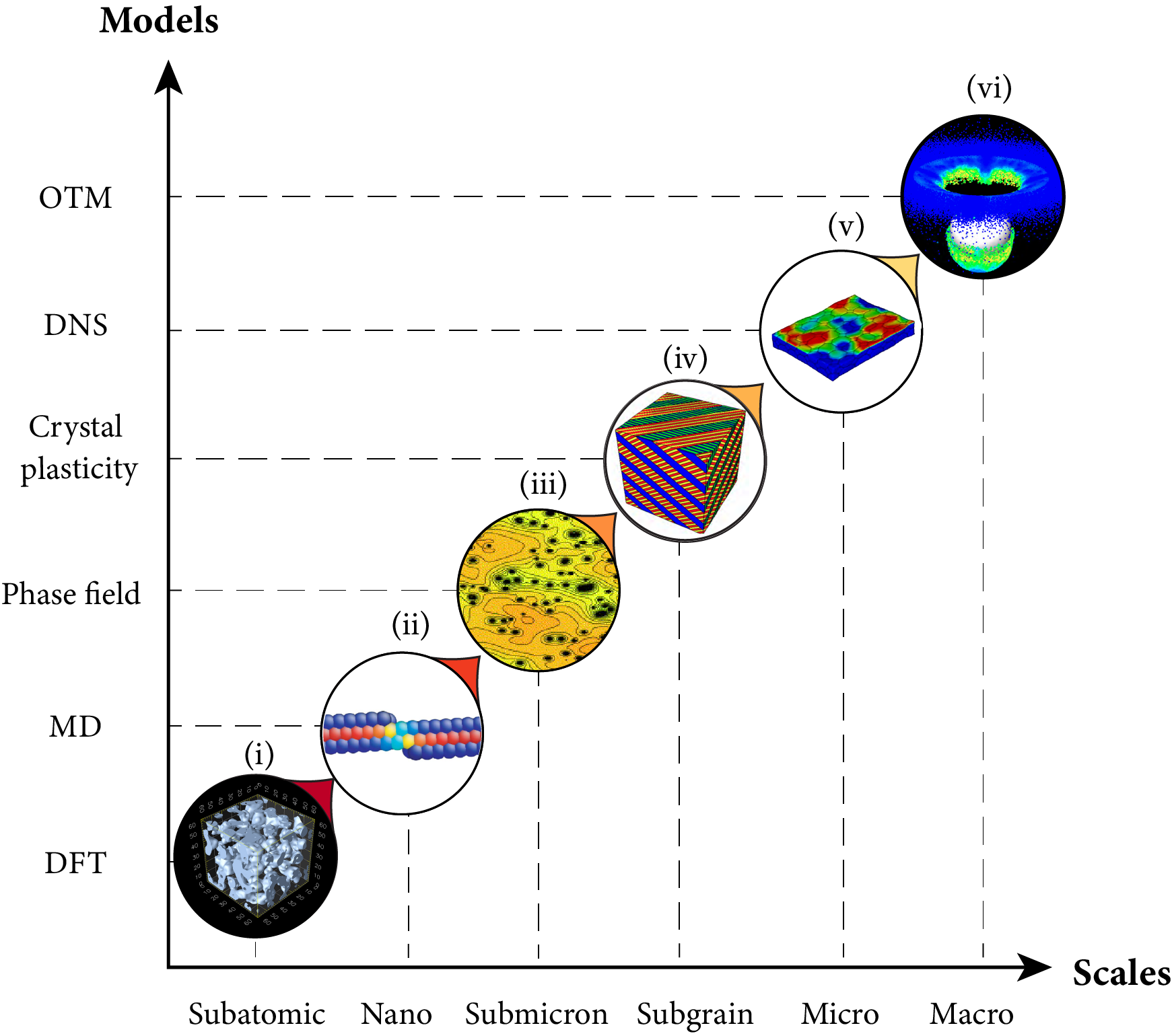
Figure 1: Example of multiscale hierarchy for modeling strength in metals. Overlaid are examples of models or calculations of several of the unit mechanisms, from bottom to top: i) density functional theory (DFT) calculations of the equation of state (EoS) in Ta (Miljacic et al., 2011); ii) molecular dynamics (MD) calculations of kink mobility in Ta (Wang et al., 2001; Segall et al., 2001; Kang et al., 2012); iii) phase-field simulations of dislocation dynamics and forest hardening (Koslowski et al., 2002); iv) lamination construction for sub-grain dislocation structures (Ortiz and Repetto, 1999); v) direct numerical simulation (DNS) of polycrystals (Zhao et al., 2004); vi) Optimal Transportation Meshfree (OTM) simulations of ballistic perforation (Li et al., 2010).

A representative hierarchy for modeling strength in metals is shown in Fig. 1 by way of example. A number of fundamental properties, such as the equations of state describing the compressibility of the material, the elastic moduli and heat capacity, can be calculated from first principles at the quantum-mechanical level up to high pressures and temperatures. Some transport properties, such as viscosity and thermal conductivity, can also be characterized from first principles, e. g., within the Green-Kubo formalism (Green, 1954; Kubo, 1957). At the nanoscale, the properties of individual lattice defects, such as vacancies and dislocations, come into focus (Leibfried and Breuer, 2006). Such properties include dislocation core energies, kink mobilities, lattice friction, short-range dislocation-dislocation interactions, vacancy formation and migration energies, grain-boundary energies, and others. The sub-micron scale is dominated by dislocation dynamics (Messerschmidt, 2010), i. e., the cooperative behavior of large dislocation ensembles, and, in the case of ductile fracture, void nucleation and cavitation. The sub-grain scale is characterized by the formation of highly-structured dislocation patterns and, in the case of metals undergoing solid-solid phase transitions, martensitic structures (Bhattacharya, 2003). This intermediate scale is important, as it underlies scaling properties such as Hall-Petch scaling, or the inverse relation between strength and the square-root of the grain size (Hall, 1951; Petch, 1953). At the microscale, ductile fracture is characterized by plastic void growth and coalescence. Finally, the macroscopic response of polycrystalline metals represents the effective behavior of large ensembles of grains (cf., e. g., (Hutchinson, 1970; Wei and Anand, 2004) for reviews).

In this work we show how, in materials for which a multiscale hierarchy is well defined, the quantification of integral uncertainties can be reduced to the analysis of each unit mechanism in turn and the propagation of unit uncertainties across the multiscale hierarchy according to an appropriate measure of interaction between the unit mechanisms. In particular, no integral calculation is required at any stage of the analysis. We specifically follow the approach of Topcu et al. (2011), which supplies rigorous upper bounds of integral uncertainties for hierarchies of interconnected subsystems through a systematic computation of moduli of continuity for each individual subsystem. The moduli of continuity supply just the right measure of interaction between the subsystems enabling the propagation of uncertainties across the hierarchy. The resulting uncertainty bounds are rigorous, i. e., they are sure to be conservative and result in safe designs; they become sharper with an increasing number of input variables (concentration-of-measure phenomenon (Talagrand, 1996)); they do not require differentiability of the subsystem response functions and account for large deviations in the response; and only require knowledge of ranges of the input parameters and not their full probability distribution, as is the case for Bayesian methods (Dashti and Stuart, 2011). In addition, the computation of the bounds is non-intrusive and can be carried out using existing deterministic models of the subsystems and external scripts.

We specifically aim to assess this hierarchical multiscale approach to uncertainty quantification (UQ) by means of an example concerned with the ballistic impact of an elastic-plastic magnesium plate struck by a heavy rigid ball. We adopt as quantity of interest the maximum backface deflection of the plate. We consider two scales of material response: a macromechanical scale characterized by the Johnson-Cook constitutive model (Johnson, 1983); and a micromechanical scale in which the polycrystalline structure of the material and its behavior at the single-crystal level are taken into account. For simplicity, we compute polycrystalline averages by means of Taylor averaging (Taylor, 1938) assuming an isotropic initial texture. The single-crystal plasticity extended to include twinning follows Chang and Kochmann (2015). We estimate ranges of parameters for the single-crystal plasticity model based on experimental data compiled from a number of sources. Calculations are carried out using the commercial finite-element package LS-DYNA (Hallquist et al., 2007) on a single converged mesh. The analysis mirrors conventional design testing for impact resistance (Mukasey et al., 2008), wherein performance is evaluated relative to a targeted set of characterized impact conditions. The hierarchical multiscale UQ protocol is implemented using the DAKOTA Version $6.12$ software package (Adams et al., 2020) of the Sandia National Laboratories.

It bears emphasis that the material model used in the calculations is intended for purposes of demonstration of the methodology and not as an accurate model of material behavior. This proviso notwithstanding, the calculations show that the integral uncertainties determined by the hierarchical multiscale UQ approach are sufficiently tight for use in engineering applications. The analysis also sheds light on the relative contributions of the different unit mechanisms to the integral uncertainty and the dominant propagation paths for uncertainty across the model hierarchy.

2 Methodology

We start with a brief review of the uncertainty quantification theory for hierarchical systems (Lucas et al., 2008; Topcu et al., 2011; Sun et al., 2020) that provides the basis for the application to multiscale material modelling pursued in this work.

2.1 McDiarmid’s inequality

We begin by considering a single-scale, or monolithic, system with uncertain inputs $x=(x_{1},...,x_{N})$ and a performance measure $y\in\real$. We assume that the inputs are independent, though not necessarily identically distributed, random variables defined on a bounded set $\mathcal{X}\subset{}^{N}$. Let ${F}:\mathcal{X}\mapsto\real$ be the response function that maps $x$ to $y$. Define the diameter of ${F}$ with respect to input $x_{i}$, $1\leq i\leq N$, as

$$d_{F,i}=\sup_{(\hat{x}_{i},x_{i}),(\hat{x}_{i},x_{i}^{\prime})\in\mathcal{X}}\big{|}{F}(\hat{x}_{i},x_{i})-{F}(\hat{x}_{i},x_{i}^{\prime})\big{|},$$ (1)

where we write

$$\hat{x}_{i}=(x_{1},\ldots,x_{i-1},x_{i+1},\ldots,x_{N}).$$ (2)

Given a performance threshold $y_{c}\in\real$, with failure occurring when $y\geq y_{c}$, the McDiarmid’s inequality (Doob, 1940) gives the following upper bound on the probability of failure

$$\mathbb{P}[y\geq y_{c}]\leq\text{exp}\bigg{(}-2\frac{M^{2}}{U^{2}}\bigg{)},$$ (3)

where $M=\text{max}(0,y_{c}-\mathbb{E}[y])$ is the design margin and

$$U=d_{F}=\bigg{(}\sum_{i=1}^{N}d_{F,i}^{2}\bigg{)}^{1/2}$$ (4)

is the system uncertainty. Thus, the system is certified if, for a given probability-of-failure tolerance $\epsilon>0$,

$$\text{exp}\bigg{(}-2\frac{M^{2}}{U^{2}}\bigg{)}\leq\epsilon,$$ (5)

or equivalently,

$$\text{CF}=\frac{M}{U}\geq\sqrt{\text{log}\sqrt{\frac{1}{\epsilon}}},$$ (6)

where CF is a confidence factor in the design (Sharp and Wood-Schultz, 2003).

We note that Eq. (3) provides a rigorous probability-of-failure upper bound for the material and, therefore, sets forth a conservative certification criterion. Importantly, no a-priori assumption on the probability distribution of the input variables, or prior, is required. The bound is uniquely determined by the design margin $M$ and the system uncertainty $U$, as unambiguously quantified by the system diameter $d_{F}$, which are both prior-free.

2.2 Hierarchical Uncertainty Quantification

As noted in the introduction, the macroscopic behavior of many material systems is the result of mechanisms over multiple scales whose functional dependencies define a graph. Conveniently, this graph structure can be exploited to divide the material response into interconnected unit mechanisms, or subsystems, and estimate integral uncertainties of the entire system from a quantification of uncertainties for each subsystem and an appropriate measure of interaction between the subsystems. We specifically follow the approach of Topcu et al. (2011), which we briefly summarize next.

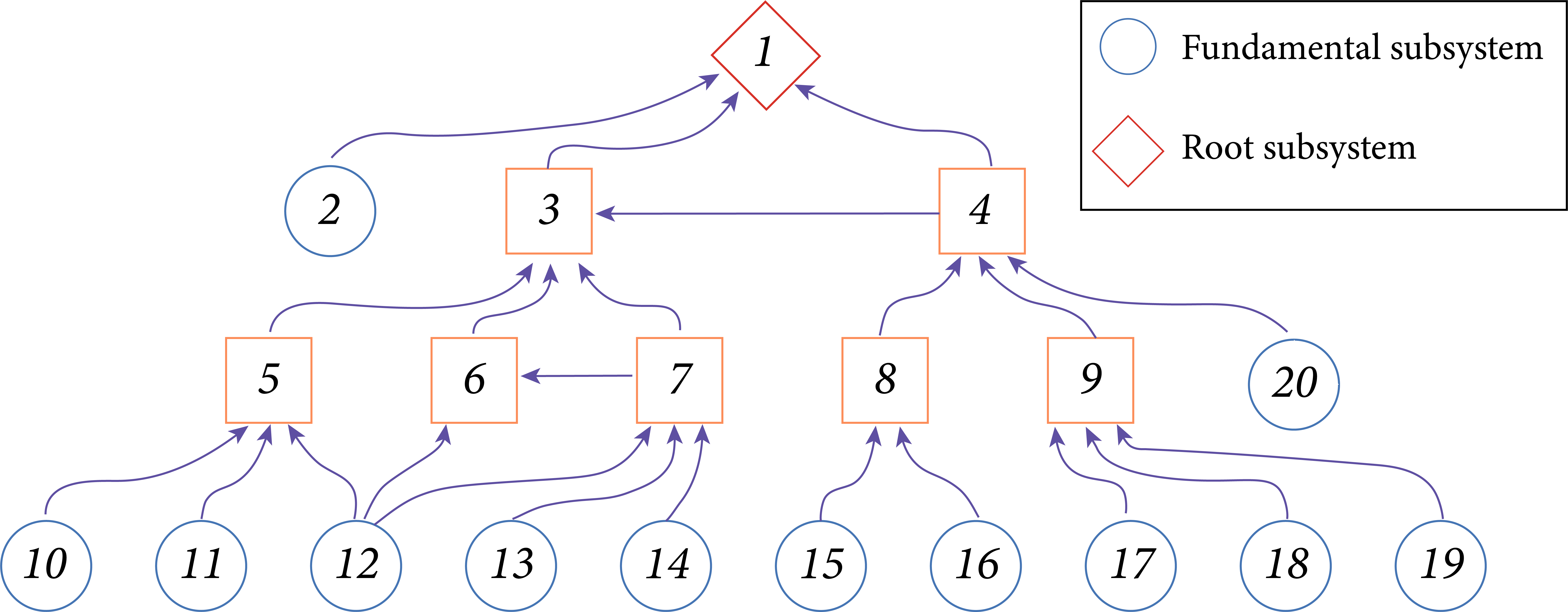
Figure 2: Graph representation of the input-output relations between the subsystems of a modular system. The nodes of the graph represent the subsystems of the system. An arrow indicates that the outputs of the subsystem at the beginning of the arrow are among the inputs of the subsystem at the end of the arrow. The subsystems represented by circular boxes do not take input from other systems and are referred to as fundamental. The system has one single root subsystem, i. e., a subsystem that does not feed into any other subsystem and through which the system output takes place.

We consider hierarchical or modular systems representable by an oriented graph $G(V,E)$ whose nodes $V$ are the subsystems and whose edges $E$ are the interfaces between the subsystems, Fig. 2. Specifically, the graph contains an oriented edge from $b$ to $a$ if the state of the subsystem $a$ depends on the state of the subsystem $b$, i. e., if the outputs of subsystem $b$ are contained among the inputs of system $a$. We then say that $a$ is an ancestor of a node $b$, denoted $a\prec b$, and that $b$ is a descendant of $a$, denoted $b\succ a$. In order to avoid circular dependencies, we assume that $G(V,E)$ is acyclic, i. e., it contains no closed-loop paths. The fundamental subsystems are those that take input from no other subsystems. We assume that the system contains a single integral subsystem that does not feed into any other subsystem. Thus, the fundamental subsystems and the integral subsystem are the leaves $V_{L}$ and the root $R$ of the graph $G(V,E)$, respectively.

Suppose that the response of subsystem $a\in V$ is characterized by a function $F_{a}:\mathcal{X}_{a}\to\mathcal{Y}_{a}$ that maps input parameters $X_{a}\in\mathcal{X}_{a}$ to outputs $Y_{a}\in\mathcal{Y}_{a}$. If $a$ is an ancestor of $b$ in the graph $G(V,E)$ then $\mathcal{Y}_{b}$ is a subspace of $\mathcal{X}_{a}$. The space of inputs of the system $\mathcal{X}$ is the Cartesian product of the input spaces of the fundamental subsystems, i. e., $\mathcal{X}=\prod_{a\in V_{L}}\mathcal{X}_{a}$. Likewise, the space of outputs of the system is $\mathcal{Y}=\mathcal{Y}_{R}$. For all subsystems other than the fundamental ones, $a\not\in V_{L}$, we have the relation $\mathcal{X}_{a}=\prod_{b\succ a}\mathcal{Y}_{b}$, i. e., the input space of subsystems $i$ is the Cartesian product of the output spaces of all its descendants. We note that non-fundamental subsystems could in principle have inputs of their own, not provided by any descendant subsystem. We accommodate such cases within the present framework simply by adding a fundamental subsystem whose response function is the identity mapping and which supplies the requisite additional inputs.

Algorithm 1 Hierarchical System Evaluation

0:  Graph $G(V,E)$; leaves $V_{L}$; root $R$; response functions $F_{a}:\mathcal{X}_{a}\to\mathcal{Y}_{a}$, $a\in V$; input $X\in\mathcal{X}$.

  i) Initialize: $V_{0}=V_{L}$, $k=0$.

  ii) Reset: $V_{k+1}=\{a\in V:\ b\in\cup_{l=0}^{k}V_{l},\ \forall b\succ a\}$.

  for all $a\in V_{k+1}$ do

     Compute $X_{a}=\big{(}F_{b}(X_{b}),\ b\succ a\big{)}$.

  end for

  if $V_{k+1}=\{R\}$ then

     return $Y=F_{R}(X_{R})$, exit.

  else

     $k\leftarrow k+1$, goto ii).

  end if

The function $F:\mathcal{X}\to\mathcal{Y}$ that describes the response of the integrated system can be evaluated recursively by means of Algorithm 1. The algorithm sets forth an “information wave” through the graph that propagates information from the leaves to the root. Thus, in the example of Fig. 2, the sequence of active subsystems is $V_{0}=\{2,10,11,12,13,14,15,16,17,18,19,20\}$, $V_{1}=\{5,7,8,9\}$, $V_{2}=\{6,4\}$, $V_{3}=\{3\}$ and $V_{5}=\{1\}$. Correspondingly, the sequence of subsystem outputs is $(Y_{5},Y_{7},Y_{8},Y_{9})$, $(Y_{6},Y_{4})$, $Y_{3}$ and $Y=Y_{1}$.

Let $\{V_{k},k=0,\dots,N\}$ be the sequence of nodal sets generated during the evaluation of the integrated response function $F(X)$, with $V_{0}=V_{L}$ and $V_{N}=\{R\}$. Define $\mathcal{X}_{k}=\prod_{a\in V_{k}}\mathcal{X}_{a}$ and $\mathcal{Y}_{k}=\prod_{a\in V_{k+1}}\mathcal{X}_{a}$, i. e., the combined sets of inputs and outputs for each iteration. We note that $\mathcal{X}=\mathcal{X}_{0}$, $\mathcal{Y}_{k}=\mathcal{X}_{k+1}$. Without loss of generality we may assume that $\mathop{\rm dim}\mathcal{Y}_{N}=\mathop{\rm dim}\mathcal{Y}=1$. Define further $F_{k}:\mathcal{X}_{k}\to\mathcal{Y}_{k}$ as $F_{k}(X_{k})=(F_{a}(X_{a}),a\in V_{k})$, $X_{k}\in\mathcal{X}_{k}$, i. e., as the forward map for iteration $k$. By these definitions and reorganization of the data, we have the composition rule

$$F=F_{N}\circ\cdots\circ F_{0}.$$ (7)

Conveniently, the propagation of uncertainty under composition is controlled by the moduli of continuity of the response functions. Recall that, given a function $f:\mathbb{R}^{n}\to\mathbb{R}^{m}$, a real number $\delta>0$ and a subset $A\subset\mathbb{R}^{n}$, the modulus of continuity $\omega_{ij}(f,\delta,A)$ of $f_{i}(x)$ with respect to $x_{j}$ over $A$ is defined as (Efimov, 2001; Steffens, 2006)

$$\begin{split}&\omega_{ij}(f,\delta,A)=\sup\{|f_{i}(x)-f_{i}(x^{\prime})|\ :\ x,x^{\prime}\in A,\ x_{k}=x^{\prime}_{k}\;\text{for}\;k\not=j,\ |x_{j}-x^{\prime}_{j}|\leq\delta\}.\end{split}$$ (8)

Thus, $\omega_{ij}(f,\delta,A)$ measures the variation of the function $f_{i}(x)$ over $A$ when the variable $x_{j}$ is allowed to deviate by less than $\delta$. We note that this component-wise definition of the modulus of continuity does not require the range or image of the function $f$ to be a normed space. This is important in practice, since the inputs and outputs of subsystems often comprise variables measured in different units which belong to vector spaces with no natural norm. Consider now two functions $f:A\subset\mathbb{R}^{n}\to\mathbb{R}^{m}$ and $g:B\subset\mathbb{R}^{m}\to\mathbb{R}^{p}$, with $B$ a hyper-rectangle such that $f(A)\subset B$, and let $\delta>0$. Let $g\circ f:A\subset\mathbb{R}^{n}\to\mathbb{R}^{p}$ be the composition of the $f$ and $g$, i. e., $(g\circ f)(x)=g(f(x))$. Then, we have (Topcu et al., 2011)

$$\omega_{ij}(g\circ f,\delta,A)\leq\sum_{k=1}^{m}\omega_{ik}(g,\omega_{kj}(f,\delta,A),B).$$ (9)

This inequality shows that the moduli of continuity of a composite function $g\circ f$ can be estimated conservatively from the moduli of continuity of the individual functions.

Algorithm 2 Hierarchical Uncertainty Quantification

0:  Graph $G(V,E)$; leaves $V_{L}$; root $R$; response functions $F_{a}:\mathcal{X}_{a}\to\mathcal{Y}_{a}$, $a\in V$; set $A\subset\mathcal{X}_{0}=\mathcal{X}$.

  for all $j=1,\dots,{\rm dim}\mathcal{X}_{0}$ do

     Compute: $D_{j}=\sup\{|x_{j}-x^{\prime}_{j}|:\ x,x^{\prime}\in A,\ x_{k}=x_{k}^{\prime},\text{ for }k\neq j\}$.

     Compute: $D_{ij}^{(0)}=\omega_{ij}(F_{0},D_{j},A),\ i=1,\dots,\mathop{\rm dim}\mathcal{Y}_{0}$.

  end for

  for all $k=1,\dots,N$ do

     Find hyper-rectangles $B_{k}\subset\mathcal{X}_{k}$ containing $(F_{k-1}\circ\cdots\circ F_{0})(A)$.

     Compute: $D_{ij}^{(k)}=\sum_{l=1}^{\mathop{\rm dim}\mathcal{X}_{k}}\omega_{il}(F_{k},D_{lj}^{(k-1)},B_{k}),\ i=1,\dots,\mathop{\rm dim}\mathcal{Y}_{k}$.

  end for

  return $\{D_{F,i}=D_{1i}^{(N)},\ i=1,\dots,{\rm dim}\mathcal{X}\}$.

This property of the moduli of continuity in turn enables uncertainties of the integral system to be bounded once the uncertainties of the subsystems and their interfaces are known. The systematic application of estimate (9) to the graph $G(V,E)$ is described in Algorithm 2 and results in a set of approximate diameters $\{D_{F,i},\ i=1,\dots,{\rm dim}\mathcal{X}\}$. The fundamental theorem proven by Topcu et al. (2011) is that the approximate diameters $\{D_{F,i}\}$ bound above the exact integral diameters $\{d_{F,i}\}$, Eq. (1), i. e.,

$$d_{F,i}\leq D_{F,i},\ i=1,\dots,{\rm dim}\mathcal{X}.$$ (10)

By the monotonicity of McDiarmid’s inequality, with respect to the diameters, it follows that replacing $\{d_{F,i}\}$ by $\{D_{F,i}\}$ in (4) and (5) results in probabilities of integral outcomes and, by extension, in conservative certification criteria.

It bears emphasis that every step of Algorithm 2 requires the execution of subsystem tests only, and that at no time during the analysis an integral test is required. The sequence $D_{ij}^{(k)}$ generated by the algorithm may be regarded as a measure of uncertainty in the $i$th output variable due to the variability of the $j$th input variable after $k$ levels of operation of the system. The algorithm propagates uncertainties in the input variables associated with a leaf $i$ through possibly multiple paths connecting the node $i$ with the root $R$. The algorithm additionally identifies the path responsible for most of the uncertainty of the integral outcome with respect to the variable $i$, namely, the path with the highest flow of uncertainty.

3 Test case: Sub-ballistic impact of magnesium plate

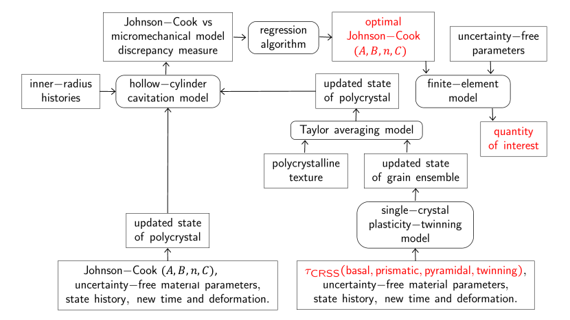
Figure 3: Graph representation of the hierarchical multiscale model of ballistic impact. Highlighted in red are the micro and mesomechanical parameters assumed to be uncertain in the UQ analysis.

As just shown in the foregoing, the integral uncertainty for a hierarchical multi-scale system can be evaluated from the moduli of continuity of the sub-system maps without integral testing. We proceed to demonstrate the feasibility of the approach by means of an example of application concerning the ballistic impact of a magnesium plate. For purposes of this demonstration, we restrict attention to three length scales as depicted in Fig. 3: i) the microscale, where the behavior of the magnesium, including slip and twinning, is modelled at the single crystal level; ii) the mesoscale, where the polycrystalline response is computed using Taylor averaging and the single-crystal model; and iii) the macroscopic impact problem, where the material behavior is approximated by the Johnson-Cook constitutive model and the ballistic performance of the magnesium plate is simulated using finite elements.

For purposes of illustration of the UQ methodology, we assume that all parameters are uncertainty-free save those shown in red in Fig. 3, namely the micromechanical critical resolved shear stresses (CRSS) for the basal slip, prismatic slip, pyramidal slip and twinning mechanisms, the mesomechanical Johnson-Cook parameters and the integral quantity of interest. These assumptions lead to the following simplified two-level hierarchical system:

$$\mathcal{X}_{0}\stackrel{{\scriptstyle F_{0}}}{{\longrightarrow}}\mathcal{Y}_{0}=\mathcal{X}_{1}\stackrel{{\scriptstyle F_{1}}}{{\longrightarrow}}\mathcal{Y}_{R},$$ (11)

cf. Fig. 3. Thus, the graph $V$ of the system contains three nodes, denoted $\{{\rm micro}\equiv 0,\ {\rm meso}\equiv 1,\ {\rm macro}\equiv R\}$, and

• Uncertain single-crystal model parameters: (CRSS) for the basal slip, prismatic slip, pyramidal slip and twinning mechanisms.

• Mapping that returns an optimal set $\mathcal{Y}_{0}$ of Johnson-Cook parameters $(A,B,n,C)$ for a given realization of $\mathcal{X}_{0}$, obtained by performing regression on stress paths computed using both the Johnson-Cook model and the single crystal model combined with Taylor averaging along selected strain paths.

• $\mathcal{X}_{1}=$ Optimal Johnson-Cook parameters.

• Finite element model of ballistic impact of magnesium plate using the Johnson-Cook model with optimal parameters $\mathcal{X}_{1}$.

• Quantity of interest extracted from the results of the finite element calculations.

A brief description of the different subsystems is given next, followed by a specification of the maps $F_{0}$ and $F_{1}$.

3.1 Micromechanical model

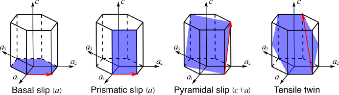
Figure 4: Schematic view of the slip and twin systems of magnesium considered in the present work. Blue planes represent the slip/twin planes, while red arrows represent the corresponding Burgers vector/twinning shear direction.

We specifically model single-crystal magnesium within the framework of finite-deformation single crystal plasticity extended to include twinning following Chang and Kochmann (2015). The reader is referred to the original publication for details of the model. The model accounts for basal slip, prismatic slip, pyramidal slip and tensile twinning, cf. Fig. 4. The entire collection of parameters of the model is listed in Table 1, including the values of the parameters determined by Chang and Kochmann (2015). For each slip system $\alpha$, ${\sigma}_{\alpha}^{\infty}$ is the ultimate strength, $h_{\alpha}$ is the self-hardening modulus, $m_{\alpha}$ is the slip rate sensitivity exponent, $\dot{\gamma}_{0,\alpha}$ is a reference slip rate and $h_{ij}$ are off-diagonals latent hardening moduli. For twinning, $h_{\beta}$ is the self-hardening modulus, $m_{\beta}$ is the rate-sensitivity exponent, $\dot{\lambda}_{0,\beta}$ is a reference twin volume-fraction rate, $\gamma_{t}$ denotes the twin strain and $k_{ij}$ are interaction moduli. In addition, the elasticity is assumed to be isotropic with Lamé constants $\lambda_{e}$ and $G$.

Table 1: Parameters of the single-crystal magnesium model.

	Parameter	Value	Unit
Basal $\langle a\rangle$	$h_{\alpha}$	7.1	GPa
	${\sigma}_{\alpha}^{\infty}$	0.7	MPa
	$h_{ij}$	0	MPa
	$m_{\alpha}$	0.05	-
	$\dot{\gamma}_{0,\alpha}$	1.0	$\text{s}^{-1}$
Prismatic $\langle a\rangle$	$h_{\alpha}$	40	GPa
	${\sigma}_{\alpha}^{\infty}$	170	MPa
	$h_{ij}$	20	MPa
	$m_{\alpha}$	0.05	-
	$\dot{\gamma}_{0,\alpha}$	1.0	$\text{s}^{-1}$
Pyramidal $\langle c+a\rangle$	$h_{\alpha}$	30	GPa
	${\sigma}_{\alpha}^{\infty}$	200	MPa
	$h_{ij}$	25	MPa
	$m_{\alpha}$	0.05	-
	$\dot{\gamma}_{0,\alpha}$	1.0	$\text{s}^{-1}$
Tensile twin	$h_{\beta}$	7	MPa
	$k_{ij}$	40	GPa
	$m_{\beta}$	0.05	-
	$\dot{\lambda}_{0,\beta}$	1.0	$\text{s}^{-1}$
	$\gamma_{t}$	0.129	-
Elastic Lame Moduli	$\lambda_{e}$	24	GPa
	$G$	25	GPa

We assume that the target plate is made of polycrystalline magnesium and compute the polycrystalline response of the polycrystal from the single crystal model just outline by means of Taylor averaging (Taylor, 1938). The computational cost of Taylor averaging is relatively small compared to other averaging schemes such as periodic boundary conditions (Geers et al., 2010). In addition, Chang and Kochmann (2015) have demonstrated good agreement between Taylor averaging and experimental measurements when the number of the grains is sufficiently large ($>100$). In calculations we assume initial isotropic texture with grain orientation matrix drawn uniformly from the Haar measure on $SO(3)$ (Haar, 1933). A total of 128 grains are used in the current study for the mesoscale model.

3.2 Johnson-Cook model

The combination of a single-crystal model and Taylor averaging just described, together with suitable initial conditions, enables the calculation of Cauchy stress histories $\sigma(t)$ at a material point from known deformation gradient histories $F(t)$. However, such calculations are computationally intensive and cannot be carried out on-the-fly as part of large-scale finite-element calculations. Instead, in said calculations we choose to use a simpler and faster surrogate or mesomechanical model.

For definiteness, we specifically choose the Johnson-Cook model (Johnson, 1983)

$$\sigma_{M}\big{(}\epsilon_{p},\dot{\epsilon}_{p})=\big{[}A+B\epsilon_{p}^{n}\big{]}\big{[}1+C\ln\dot{\epsilon}_{p}^{*}\big{]},$$ (12)

as mesomechanical model, where $\sigma_{M}=\sqrt{\nicefrac{{3}}{{2}}s\cdot s}$ is the Mises stress and $s=\sigma-\nicefrac{{1}}{{3}}\text{tr}(\sigma)I$ denotes the deviatoric part of the Cauchy stress $\sigma$, $\epsilon_{p}$ denotes the equivalent plastic strain, $\dot{\epsilon}_{p}$ is the plastic strain rate and $\dot{\epsilon}_{p}^{*}=\dot{\epsilon}_{p}/\dot{\epsilon}_{p0}$ is a normalized plastic strain rate using reference $\dot{\epsilon}_{p0}$. The model parameters are the strength $A$, the hardening modulus $B$, the strain-hardening exponent $n$, and the rate-sensitivity modulus $C$, or $\mathcal{X}_{1}=(A,B,n,C)$.

3.3 Micro-mesomechanical parameter map

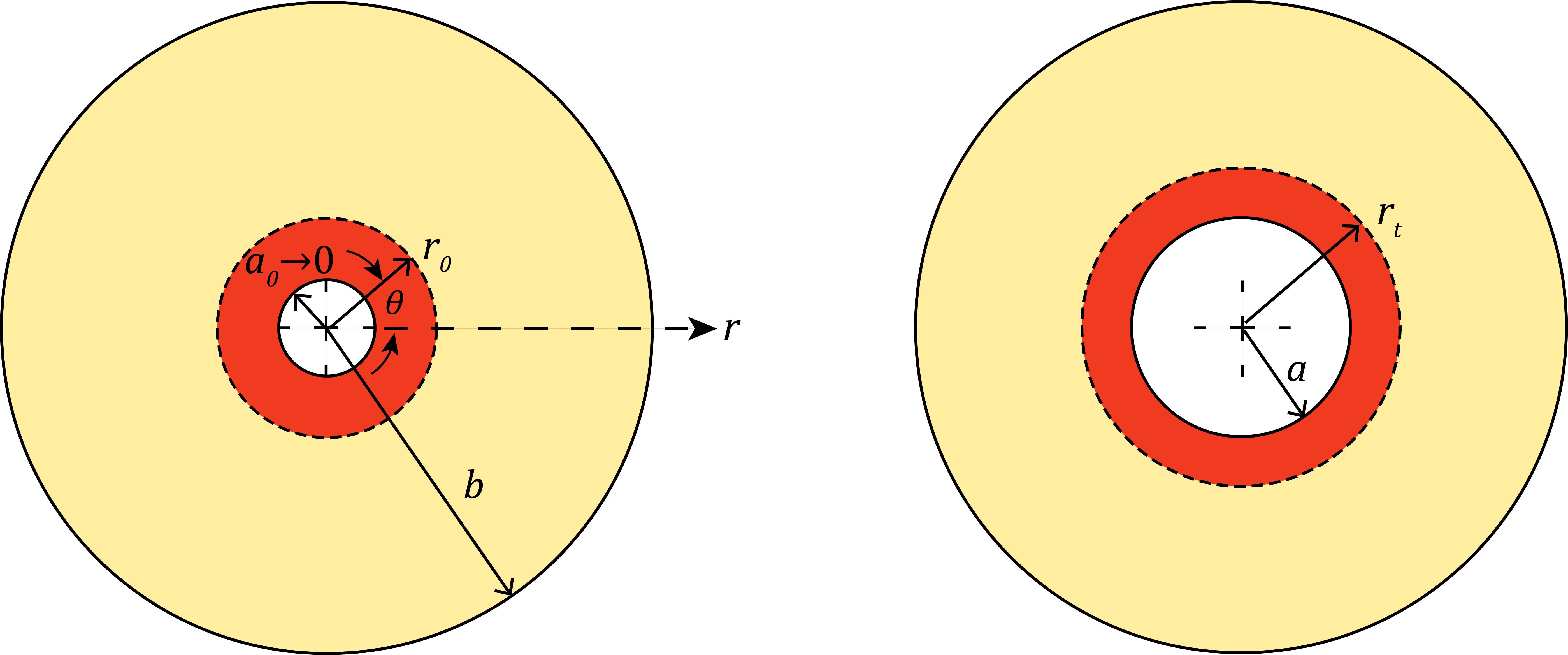
Figure 5: Schematic illustration of the plain-strain cavity expansion problem used to generate representative stress and strain histories for purposes of regression.

We now describe the function $F_{0}$ that returns the optimal value $\mathcal{Y}_{0}$ of the mesoscopic model parameters from given micromechanical model parameters $\mathcal{X}_{0}$. We understand optimality in the sense of achieving the closest agreement between the mesomechanical and the micromechanical models over selected deformation histories.

In order to generate histories for purposes of regression, we exercise the micromechanical and mesomechanical Johnson-Cook models under conditions corresponding to a plane-strain cavity expansion model, Fig. 5. Expanding cavity solutions have been commonly used to approximate conditions that arise in ballistic penetration (Bishop et al., 1945; Hanagud and Ross, 1971; Forrestal et al., 1988). We specifically consider the expansion of a solid cylinder of radius $b$ at time $t=0$ to a hollow cylinder of internal radius $a(t)=ct$ at time $t$ at constant rate $c$. Following Bishop et al. (1945) we assume that the material is incompressible, whereupon the logarithmic strains in the cylindrical coordinate system $(r,\theta)$ follow as

$$\varepsilon_{rr}(r,t)=-\varepsilon_{\theta\theta}(r,t)=\text{ln}\frac{r}{\sqrt{r^{2}+a^{2}(t)}}\quad\text{and}\quad\varepsilon_{zz}(r,t)=0,$$ (13)

and the logarithmic strain rate as

$$\dot{\varepsilon}_{rr}(r,t)=-\frac{ca}{r^{2}+a^{2}(t)}.$$ (14)

A straightforward calculation gives the Mises equivalent stress from the Johnson-Cook solution as

$$\sigma_{\text{eq}}^{\text{JC}}(r,t)=\begin{cases}\sqrt{\frac{2}{3}}E\,\text{ln}(\frac{a^{2}(t)+r^{2}}{r^{2}}),&\sigma_{\text{eq}}\leq\sigma_{0}(r,t),\\ \Big{(}A+B(\sqrt{\frac{2}{3}}\text{ln}(\frac{a^{2}(t)+r^{2}}{r^{2}})\Big{)}^{n}\,\Big{(}1+C\text{ln}(\frac{2ca}{\sqrt{3}\dot{\varepsilon}_{p0}(r^{2}+a^{2}(t))})\Big{)},&\text{otherwise},\end{cases}$$ (15)

where

$$\sigma_{0}(r,t)=A\,\Big{(}1+C\text{ln}(\frac{2ca}{\sqrt{3}\dot{\varepsilon}_{p0}(r^{2}+a^{2}(t))})\Big{)},$$ (16)

is the Mises effective stress at first yield and $E$ is the Young’s modulus. We then measure the discrepancy between the micromechanical and Johnson-Cook models in the root-mean square (RMS) sense

$${\rm Error}(\mathcal{Y}_{0}^{\rm trial}|\mathcal{X}_{0})=\Big{(}\sum_{c}\int_{0}^{b}\int_{0}^{T}|\sigma_{\text{eq}}(r,t)-\sigma_{\text{eq}}^{\text{JC}}(r,t)|^{2}\,dt\,dr\Big{)}^{1/2},$$ (17)

where the sum is carried out over a representative sample of expansion rates $c$, $\sigma_{\text{eq}}^{\text{JC}}(r,t)$ is the Mises equivalent stress computed using Johnson-Cook with parameters $\mathcal{Y}_{0}^{\rm trial}$ and $\sigma_{\text{eq}}(r,t)$ is the target Mises equivalent stress computed using the micromechanical model with parameters $\mathcal{X}_{0}$. The optimal Johnson-Cook parameters $\mathcal{Y}_{0}$ then follow by minimization of ${\rm Error}(\cdot|\mathcal{X}_{0})$, i. e.,

$$\mathcal{Y}_{0}={\rm argmin}\,{\rm Error}(\cdot|\mathcal{X}_{0}).$$ (18)

This step concludes the regression algorithm and the definition of the sought micro-to-mesomechanical mapping $F_{0}:\mathcal{X}_{0}\to\mathcal{Y}_{0}$.

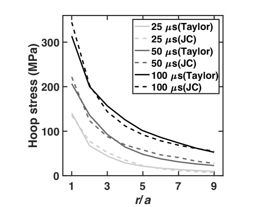
Figure 6: Comparison between the radial distributions of hoop stress $\sigma_{\theta\theta}$ computed from the micromechanical (Taylor) and the Johnson-Cook (JC) calculations.

In calculations, we employ generic algorithms (GA) (Mitchell, 1998) to solve the minimization problem. The integrals in (17) are computed by discretizing the spatial and temporal spaces. We specifically consider a cylinder radius $b=0.1$ mm, a single expansion rate $c=100.0$ mm/s, a maximum loading time $T=100.0~{}\mu$s and set the Young’s modulus to $27.0$ GPa and the reference strain rate $\dot{\epsilon}_{p0}=1.0$ s^-1. Fig. 6 illustrates the good agreement that is achieved between the micromechanical and the Johnson-Cook model with $A=20.98$ MPa, $B=161.84$ MPa, $n=0.346$ and $C=0.430$. The maximum logarithmic strain attained in the calculations is $0.35$ and the maximum logarithmic strain rate is $5,000.0$ s^-1, which provide adequate coverage of the conditions that arise in the ballistic calculations.

3.4 Meso-macromechanical forward solver

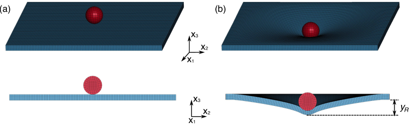
Figure 7: Schematic illustration of magnesium plate struck by a spherical steel projectile at a sub-ballistic speed. (a) Initial setup. (b) Dynamic indentation process with maximum back surface deflection labeled as $\mathcal{Y}_{R}$. In each subfigure, the top figure shows a perspective view of the projectile/plate system, and the bottom figure shows the cross-sectional view.

For purposes of illustration, we consider the problem of assessing the sub-ballistic performance of a magnesium plate struck by a spherical steel projectile. The problem is solved using the explicit dynamics solver available within the commercial software LS-DYNA (Hallquist et al., 2007) and the Johnson-Cook material model. For definiteness, we choose the maximum back surface deflection as the outcome quantity of interest $\mathcal{Y}_{R}$. For every sample Johson-Cook parameter set $\mathcal{X}_{1}$ the calculations return one value of $\mathcal{Y}_{R}$ and thus define a mapping

$$\mathcal{Y}_{R}=F_{1}(\mathcal{X}_{1}),$$ (19)

which completes the hierarchical model (11).

Table 2: Fixed material parameters used in the LS-DYNA simulation. The Gruneisen parameters of the magnesium are provided by Feng et al. (2017).

	Parameter	Value	Unit
Target (magnesium)	Mass density	$1.77$	g/$\text{cm}^{3}$
	Young’s modulus	$27.0$	GPa
	Poisson’s ratio	$0.35$	-
	Specific heat	$1.04$	J/(K$\cdot$g)
	Gruneisen intercept	$4520.0$	m/s
	Gruneisen gamma	$1.54$	-
	Gruneisen slope	$1.242$	-
Projectile (steel)	Mass density	$7.83$	g/$\text{cm}^{3}$
	Young’s modulus	$210.0$	GPa
	Poisson’s ratio	$0.30$	-

A schematic of the finite-element model is shown in Fig. 7. The diameter of the projectile is $1.12$ cm, and the size of the plate is $10\times 10\times 0.35$ cm. The attack velocity is $200$ m/s with normal impact. The backface nodes of the target near the edges are fully constrained to prevent displacement in all directions. The projectile is resolved using $864$ elements, while the number of elements for the plate is $70,000$. All the elements are linear hex with single-point integration. The time-step size is adaptive and determined by the critical size of elements, with all simulations running for $500.0~{}\mu\text{s}$ before termination. This simulation duration is sufficiently long to allow for the rebound and separation of the projectile from the plate in all the calculations. The calculations are adiabatic with the initial temperature set at room temperature. The equation-of-state, which controls the volumetric response of the material, is assumed to be of the Gruneisen type. For simplicity, the projectile is assumed to be rigid and uncertainty-free. All other material parameters are fixed and listed in Table 2.

3.5 Implementation of Hierarchical UQ

Table 3: Experimentally reported CRSS at room temperature for slip and twin systems in pure magnesium single crystals. The unit is MPa.

	CRSS	Source
Basal $\langle a\rangle$	$[0.44~{}0.58]$	Yoshinaga and Horiuchi (1964)
	$0.48$	Akhtar and Teghtsoonian (1969)
	$0.52$	Herring and Meshii (1973)
	$0.76$	Burke and Hibbard (1952)
	$0.81$	Schmid (1931)
	$4.16$	Chapuis and Driver (2011)
Prismatic $\langle a\rangle$	$17.0$	Yoshinaga and Horiuchi (1964)
	$39.0$	Reed-Hill and Robertson (1957)
	$50.0$	Flynn et al. (1961)
Pyramidal $\langle c+a\rangle$	$[27.76~{}49.22]$	Obara et al. (1973)
	$44.0$	Byer et al. (2010)
	$[52.87~{}58.52]$	Ando et al. (2007)
	$[55.48~{}86.0]$	Kitahara et al. (2007)
Tensile twin	$1.86$	Roberts (1960)
	$[3.0,11.7]$	Chapuis and Driver (2011)

Table 4: Lower and upper bounds for the CRSS in different slip and twin systems. The unit is MPa.

Basal $\langle a\rangle$	Prismatic $\langle a\rangle$	Pyramidal $\langle c+a\rangle$	Tensile twin
$[0.44~{}4.16]$	$[17.0~{}50.0]$	$[27.76~{}86.0]$	$[1.86~{}11.7]$

As already mentioned, for purposes of illustration we assume that all uncertainty in the single-crystal parameters arises from imperfect knowledge of the critical resolved shear stresses (CRSSs) in the slip and twin systems, i. e., basal $\langle a\rangle$, prismatic $\langle a\rangle$, pyramidal $\langle c+a\rangle$ and tensile twin cf. Fig. 4. These CRSSs are allowed to vary over a certain range in order to cover the experimental data. Table 3 lists a compilation of CRSS values reported in the literature for the slip and twin systems in pure magnesium single crystals at room temperature. Based on these data, the ranges of CRSSs used as the input in the multiscale UQ analysis are listed in Table 4. All other material parameters in the crystal-plasticity model are fixed and listed in Table 1.

The calculation of the diameters $D_{ij}^{(k)}$ requires the solution of a global, constrained optimization problem, while the calculation of hyper-rectangles $B_{k}$ entails the solutions of two global optimization problems with regard to each output. In order to solve these optimization problems efficiently, we have developed a non-intrusive, high-performance computational framework based on DAKOTA Version $6.12$ software package (Adams et al., 2020) of the Sandia National Laboratories. We employ genetic algorithms (GA) to solve all the optimization problems involved in the UQ analysis (Mitchell, 1998; Sun et al., 2020). GA, as a global and derivative-free optimization method, offers great flexibility in applications, such as considered here, to highly non-linear non-convex problems without the availability of gradients. Another advantage of GA is its high degree of concurrency, since individuals in each iteration can be evaluated independently across multiple processors. In all the GA calculations, we choose throughout a fixed population size of $64$. The crossover rate and mutation rate are fixed at $0.8$ and $0.1$.

3.6 Results and discussion

We recall that the modular UQ analysis is a divide-and-conquer approach that enables each subsystem to be assessed independently. In keeping with this paradigm, we analyze the micro-meso and meso-macro maps independently and combine the results to determine integral uncertainty bounds for the entire system.

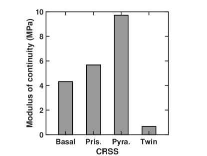
(a)

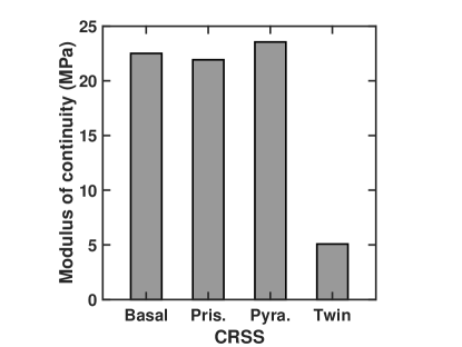
(b)

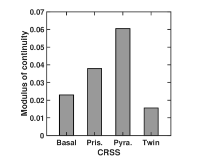
(c)

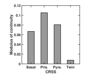
(d)

Figure 8: Moduli of continuity from single-crystal properties to Johnson-Cook (JC) parameters. (a) JC parameter $A$. (b) JC parameter $B$. (c) JC parameter $n$. (d) JC parameter $C$.

The moduli of continuity for the micro-meso mapping, relating uncertainties in the basal, prismatic, pyramidal and twin CRSS to uncertainties in the Johnson-Cook parameters are shown in Fig. 8. Clearly the micro-mechanical parameters contribute to different degrees to the uncertainties in the Johnson-Cook parameters. Remarkably, twinning uncertainty contributes the least. The parameters $A$ and $n$ are most sensitive to the pyramidal CRSS, while $C$ is most sensitive to the prismatic CRSS. By contrast, the parameter $B$ is equally sensitive to all three slip mechanisms.

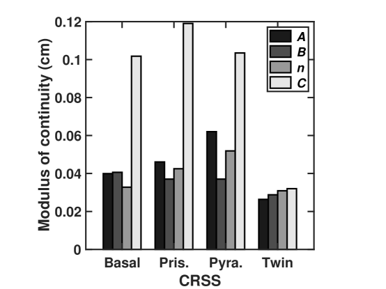
Figure 9: Moduli of continuity from single crystal properties to ballistic performance through different Johnson-Cook parameters.

The integral moduli of continuity relating uncertainties in the CRSSs to the maximum back surface deflection of the plate are shown in Fig. 9. An important property of the moduli of continuity is that, since they are dimensionally homogeneous, they can be compared and rank-ordered, which in turn provides a quantitative metric of the relative contributions of the input parameters to the overall uncertainty. In the present case, the ranking is $C>B>A>n$ for basal CRSS, $C>A>n>B$ for both prismatic and pyramidal CRSSs, and $C>n>B>A$ for twin CRSS. Remarkably, the slip uncertainty flow through the Johnson-Cook parameter $C$ is significantly larger than other paths, whereas the twin uncertainty is transmitted nearly uniformly by all Johnson-Cook parameters.

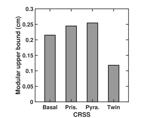
Figure 10: Sub-diameter upper bounds computed using modular approach.

Numerical results for the modular upper bounds are collected in Fig. 10. The rank-ordering of the CRSSs to the overall uncertainty in ballistic performance is found to be $\text{pyramidal}>\text{prismatic}>\text{basal}>\text{twin}$, with the pyramidal and prismatic CRSSs contributing the most, the twin CRSS the least and the basal CRSS in between. We also note that the modular upper bounds lie above the system diameters, cf. Eq. (10). Thus, the modular upper bounds provide a conservative estimate of the probability of departure from the mean when inserted into McDiarmid’s inequality Eq. (3) in place of the system diameter.

4 Concluding remarks

We have presented a framework to assess the uncertainties of a hierarchical multi-scale material system. The hierarchical structure of the multi-scale systems can be viewed as a directed graph, and we exploit this structure by bounding the uncertainty at each scale and then combining the partial uncertainties in a way that provides a bound on the overall or integral uncertainty. The bound provides a conservative estimate on the integral uncertainty. Importantly, this approach does not require integral calculations, which often are prohibitively expensive.

We have demonstrated the framework on the problem of ballistic impact of a polycrystalline magnesium plate. Magnesium and its alloys are of current interest as promising light-weight structural and protective materials. We start at the microscopic sub-grain scale where the behavior of various slip and twinning systems is described using extended crystal plasticity, pass to the mesoscopic scale of a representative volume involving multiple grains where the behavior is described using a Johnson-Cook constitutive model and study a macroscopic problem of ballistic impact of a plate. We study the uncertainty of the ballistic response due to uncertainties in the strength of individual slip and twin system.

We close with a discussion of how our approach also informs the ‘materials-by-design’ approach. In this approach, we seek to ‘design’ a material with desired properties by affecting some underlying mechanism at a fine scale. As a concrete example, consider the improvement of ballistic performance (measured by maximum deflection) of a magnesium plate. A potential way to doing so is to change the CRSS of a slip or twin system by adding solutes or precipitates. We can estimate the change in CRSS of a particular system to a solute by conducting molecular dynamics simulations. The question then, is how does this change in CRSS manifest itself in a change of ballistic performance. In the notation of (11), we seek to understand how the change of $\mathcal{X}_{0}$ affects $\mathcal{Y}_{R}$, or the modulus of continuity of this composite map. The method we have presented provides an outer bound (optimistic in the context of design) on this modulus. Importantly we can compute this bound by studying individual scales ($F_{0}$ and $F_{1}$) without the need for prohibitively expensive integral calculations.

Acknowledgement

We are grateful to Dennis Kochmann for making available to us the single-crystal and Taylor averaging codes used in this work to generate data. This research was sponsored by the Army Research Laboratory and was accomplished under Cooperative Agreement Number W911NF-12-2-0022. The views and conclusions contained in this document are those of the authors and should not be interpreted as representing the official policies, either expressed or implied, of the Army Research Laboratory or the U.S. Government. The U.S. Government is authorized to reproduce and distribute reprints for Government purposes notwithstanding any copyright notation herein.

References

- Adams et al. [2020] B. M. Adams, W. J. Bohnhoff, K. R. Dalbey, M. S. Ebeida, J. P. Eddy, M. S. Eldred, R. W. Hooper, P. D. Hough, K. T. Hu, J. D. Jakeman, M. Khalil, K. A. Maupin, J. A. Monschke, E. M. Ridgway, A. A. Rushdi, D. T. Seidl, J. A. Stephens, L. P. Swiler, and J. G. Winokur. Dakota, a multilevel parallel object-oriented framework for design optimization, parameter estimation, uncertainty quantification, and sensitivity analysis: version 6.12 user’s manual. Sandia National Laboratories, Tech. Rep. SAND2020-5001, 2020.