Another estimation of Laplacian spectrum of the Kronecker product of graphs

Abstract

The relationships between eigenvalues and eigenvectors of a product graph and those of its factor graphs have been known for the standard products, while characterization of Laplacian eigenvalues and eigenvectors of the Kronecker product of graphs using the Laplacian spectra and eigenvectors of the factors turned out to be quite challenging and has remained an open problem to date. Several approaches for the estimation of Laplacian spectrum of the Kronecker product of graphs have been proposed in recent years. However, it turns out that not all the methods are practical to apply in network science models, particularly in the context of multilayer networks. Here we develop a practical and computationally efficient method to estimate Laplacian spectra of this graph product from spectral properties of their factor graphs which is more stable than the alternatives proposed in the literature. We emphasize that a median of the percentage errors of our estimated Laplacian spectrum almost coincides with the $x$-axis, unlike the alternatives which have sudden jumps at the beginning followed by a gradual decrease for the percentage errors. The percentage errors confined (confidence of the estimations) up to $\pm$10% for all considered approximations, depending on a graph density. Moreover, we theoretically prove that the percentage errors becomes smaller when the network grows or the edge density level increases. Additionally, some novel theoretical results considering the exact formulas and lower bounds related to the certain correlation coefficients corresponding to the estimated eigenvectors are presented.

Keywords— Kronecker product of graphs, Estimated Laplacian eigenvalues and eigenvectors of graph product

1 Introduction

Many real-life interactions throughout nature and society, such as protein-protein interaction networks [1], connections among image pixels [2], Internet social networks [3], the evolution of a quantum system [4] etc., could be naturally described and represented in the context of large networks. However, the properties of such large networks can not be easily determined because of a large computational complexity of methods and algorithms performed on their corresponding graph matrices. Fortunately, large networks are often composed of several smaller pieces, for example motifs [5], communities [6], or layers [7]. In this case, by using the properties of these smaller structures, we can determine the properties of large networks obtained by using some operations [8, 9]. In graph theory there are three fundamental graph products which refer to the large network’s construction from two or more small graphs: Cartesian product, Kronecker (direct) product, and strong product. In each case, the product of graphs $G$ and $H$ is a graph whose vertex set is the Cartesian product $V(G)\times V(H)$ of sets, while each product has different rules for edge creation. Computer science is one of the many fields (such as mathematics and engineering) in which graph products, with their own set of applications and theoretical interpretations, are becoming commonplace. As one specific example, large networks such as the Internet graph, with several hundred million hosts, can be efficiently modeled by subgraphs of powers of small graphs with respect to the Kronecker product [10]. More recently, graph products have also began to appear in network science, where multiplication of graphs are often used as a formal way to describe certain types of multilayer network topologies [7][11][12]. Products of graphs that make use of spectral methods have also found important applications in interconnection networks, massively parallel computer architectures and diffusion schemes [13].

It was recognized in about the last twenty years that graph spectra have many important applications in various areas, especially in the fields of computer sciences (see, e.g., [14][15]), such as Internet technologies, computer vision, pattern recognition, data mining, multiprocessor systems, statistical databases and many others. One of the important questions to be addressed in this area, and which have been studied extensively by many researchers, is how to characterize spectral properties of a product graph using those of its factor graphs. Relationships between spectral properties of a product graph and those of its factor graphs have been known for the spectra of degree and adjacency matrices for all of the three products, as well as the Laplacian spectra for Cartesian product [16]. Results describing the adjacency matrix and its spectra of the product graphs can be also found in [17] and [18], while a complete characterization of the Laplacian spectrum of the Cartesian product of two graphs has been done by Merris [19]. In the paper [20], the authors tried to exploit the benefits of the Kronecker graph representation, which is used as a replacement for the multilayer network. However, they had to face an open problem, because the Laplacian spectrum of the Kronecker product of two graphs graphs can not be characterized by using the Laplacian spectra of the factors. In [21], the authors gave the explicit complete characterization of the Laplacian spectrum of the Kronecker product of two graphs in some particular cases. Since it seems that an explicit formula can not be obtained for the general case, in [16] the authors developed empirical methods to estimate the Laplacian spectra of the Kronecker of graphs from spectral properties of their factor graphs.

In this paper we develop an alternative practical method for an estimation of the the Laplacian spectrum and eigenvectors of the Kronecker (direct) product of two graphs. We noticed that estimated eigenvalues and eigenvectors of these approximations express different behavior depending on the type of network topology. The effectiveness of the proposed methods are evaluated through numerical experiments, where experiments are performed on three types of graphs: Erdős-Rényi, Barabási-Albert and Watts-Strogatz, while the edge density percentage is varied over 10%, 30%, and 65%. In order to see whether, our novel approximation or the one proposed by Sayama in [16], is more suitable for the original eigenvalues and eigenvectors, we compare them in the following two ways. First, we give an empirical and some theoretical evidence that the Kronecker product of eigenvectors of normalized Laplacian matrices of factor graphs can be also used as an approximation for the eigenvectors of Laplacian matrix of Kronecker product of graphs. It can be done by comparing the correlation coefficients that correspond to the approximated vectors for both approximation in regard to different types and edge density levels of graphs. Then, in order to test how close the estimated to the original eigenvalues of Laplacian of the Kronecker product of graphs for both approximations are, the difference between them in terms of a distribution of percentage errors is reported. We show that a distribution of percentage errors between novel estimated and original spectra is more stable than the error obtained for the Sayama’s spectrum and it is almost uniformly distributed around 0, all in the case of Erdős-Rényi and Watts-Strogatz random networks. It is also noticed that both approximations produced reasonable estimations of Laplacian spectra with percentage errors confined within a $\pm$10% range for most eigenvalues, with a small variations depending on the type and edge density levels of random networks. Moreover, we theoretically prove that the percentage errors become smaller when the network grows or the edge density level increases for Erdős-Rényi random networks. In the case of Barabási-Albert random networks, similar number of jumps in the graphs of percentage errors distribution is noticed for the both proposed estimated spectra.

The remainder of our paper is organized through the following sections. In Section 2 we will explain the motivation and assumptions for our alternative approach developed for the estimation of the Laplacian eigenvalues and eigenvectors of the Kronecker product of graphs. Moreover, in subsection 2.1 we recall some results and techniques used in [16] and provide a proof that all estimated eigenvalues proposed by Sayama are nonnegative. In subsection 2.2 we introduce the Kronecker product of eigenvectors of normalized Laplacian matrices of factor graphs as a potential approximation for the actual eigenvectors the Laplacian matrix of Kronecker product of graphs and by using them we get the formula (5) for estimating the Laplacian spectra of Kronecker product of graphs. In Section 3 we report a behavior of the estimated eigenvalues and eigenvectors (for both approximations) compared to the original ones with regard to the different types of graphs and different edge density levels. The comparison between estimated and original spectra has been done by calculating the percentage error, while the correlation coefficients are used to express the difference between eigenvectors. In subsection 3.1.2 we provide some new theoretical results related to the correlation coefficients that correspond to the estimated vectors for both approximation and give certain explanation why the Kronecker product of eigenvectors of normalized Laplacian matrices of factor graphs can be used as suitable approximation for the actual eigenvectors the Laplacian matrix of Kronecker product of graphs. In Theorem  1 and Theorem 2 we provide exact formulas for the certain correlation coefficients and the expected values of the correlation coefficients, respectively, corresponding to the eigenvectors proposed in [16]. From the formulas for the correlation coefficients follow that they depend only on the degrees of one of the factor graphs and hence they are mutually equal. According to the expected value of the previous correlation coefficients obtained by Theorem 2 and the inequality given by Theorem 4, we obtain that the correlation coefficients corresponding to our estimated vectors in some cases can be greater than the coefficient correlations corresponding to the eigenvectors proposed in [16]. Finally, using Theorem 5 we give a theoretical explanation of why the estimated eigenvalues for the random graphs become more accurate to the real values when the network grows or the edge density level increases. The paper concludes with a summary of key points and directions for further work. We also point out that these approximations could have a very important application in learning models based on multilayer networks. [20].

2 Proposed methods

Before describing the proposed methods, we provide definitions for concepts used throughout the paper. By $G=(V_{G},E_{G})$ we denote a simple connected graph (without loops and multiple edges), where $V_{G}$ is the set of vertices and $E_{G}\subseteq{V_{G}\choose 2}$ is a set of edges of $G$. The adjacency matrix $A$ for a graph $G$ with $N$ vertices is an $N\times N$ matrix whose $(i,j)$ entry is 1 if the $i$-th and $j$-th vertices are adjacent, and 0 if they are not. A number of the vertices $N$ of a graph $G$ is called the order of a graph $G$. A vertex and an edge are called incident, if the vertex is one of the two vertices that the edge connects. The Laplacian matrix of the adjacency matrix $A$ is defined as $L=D-A$ where $D$ is the degree matrix of $A$ (degree matrix is a diagonal matrix where each entry $(i,i)$ is equal to the number of edges incident to $i$-th vertex). The normalized Laplacian matrix is defined as $\mathcal{L}=D^{-\frac{1}{2}}LD^{-\frac{1}{2}}=I-D^{-\frac{1}{2}}AD^{-\frac{1}{2}}$. Let $G=(V_{G},E_{G})$ and $H=(V_{H},E_{H})$ be two simple connected graphs.

Definition 1

The Kronecker product of graphs denoted by $G\otimes H$ is a graph defined on the set of vertices $V_{G}\times V_{H}$ such that two vertices $(g,h)$ and $(g^{\prime},h^{\prime})$ are adjacent if and only if $(g,g^{\prime})\in E_{G}$ and $(h,h^{\prime})\in E_{H}$.

The Kronecker product of an $N\times N$ matrix $A$ and a $M\times M$ matrix $B$ is the $(NM)\times(NM)$ matrix $A\otimes B$ with elements defined by $(A\otimes B)_{I,J}=A_{i,j}B_{k,l}$ with $I=M(i-1)+k$ and $J=M(j-1)+l$.

In the rest of this section we discuss the spectral decomposition of the Laplacian of the Kronecker product of graphs from those of its factor graphs. Because it seems that such an explicit formula does not exist, we need to apply some approximations in order to obtain the estimated eigenvalues and eigenvectors.

2.1 Estimation of Laplacian spectrum of Kronecker product graph by using the Kronecker product of Laplacian eigenvectors of factor graphs

In the following section we will explain the motivation and assumptions from [16] for the proposed approximation and show some of their properties. The Laplacian of the Kronecker product of graphs is given by the following

$$\begin{split}L_{S_{1}\otimes S_{2}}&=D_{S_{1}\otimes S_{2}}-A_{S_{1}\otimes S_{2}}\\ &=(D_{S_{1}}\otimes D_{S_{2}})-(A_{S_{1}}\otimes A_{S_{2}})\\ &=D_{S_{1}}\otimes D_{S_{2}}-(D_{S_{1}}-L_{S_{1}})\otimes(D_{S_{2}}-L_{S_{2}})\\ &=L_{S_{1}}\otimes D_{S_{2}}+D_{S_{1}}\otimes L_{S_{2}}-L_{S_{1}}\otimes L_{S_{2}},\end{split}$$

where $A_{S_{1}}$ and $A_{S_{2}}$ are the adjacency matrices and $D_{S_{1}}$ and $D_{S_{2}}$ are the degree matrices of graphs $S_{1}$ and $S_{2}$, respectively, where $|S_{1}|=n_{1}$ and $|S_{2}|=n_{2}$. The idea of the proposed approximation is to assume that $w_{i}^{S_{1}}\otimes w_{j}^{S_{2}}$, where $w_{i}^{S_{1}}$ and $w_{j}^{S_{2}}$ are arbitrary eigenvectors of $L_{S_{1}}$ and $L_{S_{2}}$ respectively, could be used as a substitute for the true eigenvectors of $L_{S_{1}\otimes S_{2}}$. A motivation for this assumption came from the fact that the Laplacian spectra of the Kronecker product of graphs resemble those of the Cartesian product of graphs when either factor graph is regular [21]. Let $W_{S_{1}}$ and $W_{S_{2}}$ be $n_{1}\times n_{1}$ and $n_{2}\times n_{2}$ square matrices that contain all $w_{i}^{S_{1}}$ and $w_{j}^{S_{2}}$ as column vectors, respectively. By making (mathematically incorrect) assumption that $D_{S_{1}}W_{S_{1}}\approx W_{S_{1}}D_{S_{1}}$ and $D_{S_{2}}W_{S_{2}}\approx W_{S_{2}}D_{S_{2}}$ it can be obtained that

$$\begin{split}L_{S_{1}\otimes S_{2}}(W_{S_{1}}\otimes W_{S_{2}})&=L_{S_{1}}W_{S_{1}}\otimes D_{S_{2}}W_{S_{2}}+D_{S_{1}}W_{S_{1}}\otimes L_{S_{2}}W_{S_{2}}-L_{S_{1}}W_{S_{1}}\otimes L_{S_{2}}W_{S_{2}}\\ &\approx W_{S_{1}}\Lambda_{S_{1}}\otimes W_{S_{2}}D_{S_{2}}+W_{S_{1}}D_{S_{1}}\otimes W_{S_{2}}\Lambda_{S_{2}}-W_{S_{1}}\Lambda_{S_{1}}\otimes W_{S_{2}}\Lambda_{S_{2}}\\ &=(W_{S_{1}}\otimes W_{S_{2}})\Big{(}\Lambda_{S_{1}}\otimes D_{S_{2}}+D_{S_{1}}\otimes\Lambda_{S_{2}}-\Lambda_{S_{1}}\otimes\Lambda_{S_{2}}\Big{)},\end{split}$$ (1)

where $\Lambda_{S_{1}}$ and $\Lambda_{S_{2}}$ are diagonal matrices with eigenvalues $\mu^{S_{1}}_{i}$ of $L_{S_{1}}$ and $\mu^{S_{2}}_{j}$ of $L_{S_{2}}$, respectively. From the last equation, estimated Laplacian spectrum of $S_{1}\otimes S_{2}$ could be calculated as

$$\mu_{ij}=\{\mu_{i}^{S_{1}}d_{j}^{S_{2}}+d_{i}^{S_{1}}\mu_{j}^{S_{2}}-\mu_{i}^{S_{1}}\mu_{j}^{S_{2}}\}.$$ (2)

where $d_{i}^{S_{1}}$ and $d_{j}^{S_{2}}$ are the diagonal entries of the degree matrices $D_{S_{1}}$ and $D_{S_{2}}$, respectively.

Here we note that the orderings of $w_{i}^{S_{1}}$ and $w_{j}^{S_{2}}$ (and hence $\mu_{i}^{S_{1}}$ and $\mu_{j}^{S_{2}}$) are independent of the vertex orderings in $D_{S_{1}}$ and $D_{S_{2}}$, respectively. This can help in reducing the mathematical inaccuracy arising from the mentioned incorrect assumptions by finding optimal column permutations of $W_{S_{1}}$ and $W_{S_{2}}$ (influencing $\Lambda_{S_{1}}$ and $\Lambda_{S_{2}}$). Therefore, several types of ordering of eigenvalues ($\mu_{i}^{S_{1}}$ and $\mu_{j}^{S_{2}}$) of factor graphs were tested [16], while the degree sequences are fixed in ascending order. It was obtained that the most effective heuristic method is when the eigenvalues are sorted in ascending order.

From (2) it can be easily seen that the estimated spectrum always has an eigenvalue of 0, because if $\mu_{i}^{S_{1}}=0$ and $\mu_{j}^{S_{2}}=0$, then $\mu_{ij}=0$. However, it is not commented in [16] whether all other estimated eigenvalues $\mu_{ij}$ are greater than or equal to 0. Notice that  (2) can be rewritten as follows:

$$\mu_{i}^{S_{1}}(d_{j}^{S_{2}}-\frac{\mu_{j}^{S_{2}}}{2})+\mu_{j}^{S_{2}}(d_{i}^{S_{1}}-\frac{\mu_{i}^{S_{1}}}{2})\,\,\,\,\text{for}\,\,1\leq i\leq n_{1},\,1\leq j\leq n_{2}.$$

If a graph is regular then the absolute values of the eigenvalues of its adjacency matrix are less than or equal to the regularity of the graph (according to the Perron-Frobenius theorem, see [22], pp. 178) and it is clear from the definition of the Laplacian matrix that all Laplacian eigenvalues are less than or equal to the double value of the regularity. This implies that in the case when $S_{1}$ and $S_{2}$ are regular, we have that $d_{j}^{S_{2}}\geq\frac{\mu_{j}^{S_{2}}}{2}$ and $d_{i}^{S_{1}}\geq\frac{\mu_{i}^{S_{1}}}{2}$, and therefore $\mu_{ij}\geq 0$. In the following we prove that these eigenvalues are nonnegative in the general case.

By applying Gershgorin circle theorem on Laplacian matrix we can obtain only the inequality $d_{n_{1}}^{S_{1}}-\frac{\mu_{n_{1}}^{S_{1}}}{2}\geq 0$ (or equivalently $\mu_{n_{1}}^{S_{1}}\leq 2d_{n_{1}}^{S_{1}}$). Indeed, as every eigenvalue of the $n_{1}\times n_{1}$ Laplacian matrix $L=(l_{i,j})_{1\leq i,j\leq n_{1}}$ lies within the union of disks centered at $l_{i,i}=d_{i}^{S_{1}}$ with radius $R_{i}=d_{i}^{S_{1}}$ ($R_{i}$ is the sum of the absolute values of the non-diagonal entries in the $i$-th row for $1\leq i\leq n_{1}$), we can not conclude that every eigenvalue $\mu_{i}^{S_{1}}$ lies in the circle centered at $d_{i}^{S_{1}}$ with radius $d_{i}^{S_{1}}$, i.e. $\mu_{i}^{S_{1}}\leq 2d_{i}^{S_{1}}$, $1\leq i\leq n_{1}-1$ (see Figure 1) .

It turns out that the inequality $\mu_{i}^{S_{1}}\leq 2d_{i}^{S_{1}}$ can be proved by using Courant-Fischer theorem for every index $i$. Namely, it is easy to see that the quadratic form $x^{T}Lx$ in respect to the Laplace matrix $L$ and an arbitrary vector $x=(x_{1},x_{2},\ldots,x_{n_{1}})$ can be rewritten in the following way

$$x^{T}Lx=\sum_{j=1}^{n_{1}}d_{j}^{S_{1}}x_{j}^{2}-2\sum_{(i,j)\in E(S_{1})}x_{i}x_{j}.$$

Now, using the arithmetic-geometric mean inequality between $x_{i}$ and $x_{j}$, $|2x_{i}x_{j}|\leq x_{i}^{2}+x_{j}^{2}$, it holds that $-2\sum_{(i,j)\in E(S_{1})}x_{i}x_{j}\leq\sum_{j=1}^{n_{1}}d_{j}^{S_{1}}x_{j}^{2}$ and therefore $x^{T}Lx\leq 2\sum_{j=1}^{n_{1}}d_{j}^{S_{1}}x_{j}^{2}$. Furthermore, considering $x\in R^{i}\times\{0\}^{n-i}\subseteq R^{n}$, we have in this case that $x^{T}Lx\leq 2\sum_{j=1}^{i}d_{j}^{S_{1}}x_{j}^{2}\leq 2d_{i}^{S_{1}}\|x\|^{2}$. Finally, according to Courant-Fischer we have that $\mu_{i}^{S_{1}}\leq\max_{x\in R^{i}\times\{0\}^{n-i}}\frac{x^{T}Lx}{\|x\|^{2}}\leq\frac{2d_{i}^{S_{1}}\|x\|^{2}}{\|x\|^{2}}=2d_{i}^{S_{1}}$ (we have already mentioned that the degree sequence is set in ascending order, that is $d_{1}^{S_{1}}\leq\ldots\leq d_{n_{1}}^{S_{1}}$).

Figure 1: Gershgorin disks for Laplacian matrix

The approximations from [16] are not derived from rigorous mathematical proofs, but from empirical evidence and good behavior of estimated eigenvalues and eigenvectors has been noticed for some types of random graphs. In the following subsection we propose an estimation of Laplacian spectral decomposition for the Kronecker product of graphs by using the normalized Laplacian eigenvectors of factor graphs. We show some differences side by side (both experimentally and analytically) between these approximations through the eigenvectors and eigenvalues analysis separately.

2.2 Estimation of Laplacian spectrum of Kronecker product graph by using the Kronecker product of normalized Laplacian eigenvectors of factor graphs

In this section we propose an alternative approach for estimating the Laplacian spectrum of the Kronecker product of graphs. The idea comes from the fact that the normalized Laplacian matrix of the Kronecker product of graphs can be represented in terms of normalized Laplacian matrices of factor graphs. Moreover, in some cases the Kronecker product of the eigenvectors of $\mathcal{L}_{S_{1}}$ and $\mathcal{L}_{S_{2}}$ gives better approximation for eigenvectors of $L_{S_{1}\otimes S_{2}}$ than the Kronecker product of the eigenvectors of $L_{S_{1}}$ and $L_{S_{2}}$. Now, we will explain the motivation and assumptions for this novel approach in more detail.

By the definition of the normalized Laplacian and the property $(A\otimes B)^{-1}=A^{-1}\otimes B^{-1}$, the normalized Laplacian of the matrix $S_{1}\otimes S_{2}$ can be written in the following way

$$\mathcal{L}_{S_{1}\otimes S_{2}}=I_{n_{1}}\otimes I_{n_{2}}-(D_{S_{1}}^{-\frac{1}{2}}\otimes D_{S_{2}}^{-\frac{1}{2}})(S_{1}\otimes S_{2})(D_{S_{1}}^{-\frac{1}{2}}\otimes D_{S_{2}}^{-\frac{1}{2}}).$$

Using the property of the Kronecker product of matrices, $(A\otimes B)(C\otimes D)=AC\otimes BD$, we further obtain:

$$\mathcal{L}_{S_{1}\otimes S_{2}}=I_{n_{1}}\otimes I_{n_{2}}-(D_{S_{1}}^{-\frac{1}{2}}S_{1}D_{S_{1}}^{-\frac{1}{2}})\otimes(D_{S_{2}}^{-\frac{1}{2}}S_{2}D_{S_{2}}^{-\frac{1}{2}})=I_{n_{1}}\otimes I_{n_{2}}-(I_{n_{1}}-\mathcal{L}_{S_{1}})\otimes(I_{n_{2}}-\mathcal{L}_{S_{2}}).$$

Let $\{\lambda_{i}^{S_{1}}\}$ and $\{\lambda_{j}^{S_{2}}\}$ be the eigenvalues of the matrices $\mathcal{L}_{S_{1}}$ and $\mathcal{L}_{S_{2}}$, with the corresponding orthonormal eigenvectors $\{v_{i}^{S_{1}}\}$ and $\{v_{j}^{S_{2}}\}$, where $i=1,2,\ldots,n_{1}$ and $j=1,2,\ldots,n_{2}$. Denote by $\Lambda_{S_{1}}$ and $\Lambda_{S_{2}}$ the diagonal matrices whose diagonal elements are the values $1-\lambda_{i}^{S_{1}}$ and $1-\lambda_{j}^{S_{2}}$, respectively. Also, $V_{S_{1}}$ and $V_{S_{2}}$ stand for the square matrices which contain $v_{i}^{S_{1}}$ and $v_{j}^{S_{2}}$ as column vectors. Using the spectral decomposition of the matrix $(I_{n_{1}}-\mathcal{L}_{S_{1}})\otimes(I_{n_{2}}-\mathcal{L}_{S_{2}})$, from the above equation it follows that

$$\begin{split}\mathcal{L}_{S_{1}\otimes S_{2}}&=I_{n_{1}}\otimes I_{n_{2}}-(V_{S_{1}}\Lambda_{S_{1}}V_{S_{1}}^{T})\otimes(V_{S_{2}}\Lambda_{S_{2}}V_{S_{2}}^{T})\\ &=I_{n_{1}}\otimes I_{n_{2}}-(V_{S_{1}}\otimes V_{S_{2}})(\Lambda_{S_{1}}\otimes\Lambda_{S_{2}})(V_{S_{1}}\otimes V_{S_{2}})^{T}\\ &=(V_{S_{1}}\otimes V_{S_{2}})(I_{n_{1}}\otimes I_{n_{2}}-\Lambda_{S_{1}}\otimes\Lambda_{S_{2}})(V_{S_{1}}\otimes V_{S_{2}})^{T},\end{split}$$ (3)

since $(V_{S_{1}}\otimes V_{S_{2}})(V_{S_{1}}\otimes V_{S_{2}})^{T}=I_{n_{1}n_{2}}$. This further implies that the normalized Laplacian matrix of the Kronecker product of graphs have $\{1-(1-\lambda_{i}^{S_{1}})(1-\lambda_{j}^{S_{2}})\}$ as eigenvalues and $\{v_{i}^{S_{1}}\otimes v_{j}^{S_{2}}\}$ as eigenvectors.

Now, put $\Lambda=I_{n_{1}}\otimes I_{n_{2}}-\Lambda_{S_{1}}\otimes\Lambda_{S_{2}}$ and $D=D_{S_{1}}\otimes D_{S_{2}}$. It is well known that the normalized Laplacian can be expressed in term of Laplacian matrix as $\mathcal{L}=D^{-\frac{1}{2}}LD^{-\frac{1}{2}}$. Furthermore, as $L_{S_{1}\otimes S_{2}}(V_{S_{1}}\otimes V_{S_{2}})=D^{\frac{1}{2}}\mathcal{L}_{S_{1}\otimes S_{2}}D^{\frac{1}{2}}(V_{S_{1}}\otimes V_{S_{2}})$, using the similar assumption like in the previous subsection that $D_{S_{1}}^{\frac{1}{2}}V_{S_{1}}\approx V_{S_{1}}D_{S_{1}}^{\frac{1}{2}}$ and $D_{S_{2}}^{\frac{1}{2}}V_{S_{2}}\approx V_{S_{2}}D_{S_{2}}^{\frac{1}{2}}$, from (3), we derive

$$L_{S_{1}\otimes S_{2}}(V_{S_{1}}\otimes V_{S_{2}})\approx D^{\frac{1}{2}}\mathcal{L}_{S_{1}\otimes S_{2}}(V_{S_{1}}\otimes V_{S_{2}})D^{\frac{1}{2}}=D^{\frac{1}{2}}\Lambda(V_{S_{1}}\otimes V_{S_{2}})D^{\frac{1}{2}}.$$

Finally, applying the same assumption again we have the following formula

$$L_{S_{1}\otimes S_{2}}(V_{S_{1}}\otimes V_{S_{2}})\approx(D\Lambda)(V_{S_{1}}\otimes V_{S_{2}}).$$ (4)

Inside the first pair of parenthesis of the right-hand side of (4) is the diagonal matrix $D\Lambda$ which leads us to a potential formula for estimating the Laplacian spectrum of the Kronecker product of graphs, while for the corresponding eigenvectors we could use eigenvectors of the normalized Laplacian matrix of the Kronecker product of graphs. Therefore, a potential formula for estimating the Laplacian spectra of the Kronecker product of graphs

$$\begin{split}\mu_{ij}&=\{(1-(1-\lambda_{i}^{S_{1}})(1-\lambda_{j}^{S_{2}}))d_{i}^{S_{1}}d_{j}^{S_{2}}\}\\ &=\{(\lambda_{i}^{S_{1}}+\lambda_{j}^{S_{2}}-\lambda_{i}^{S_{1}}\lambda_{j}^{S_{2}})d_{i}^{S_{1}}d_{j}^{S_{2}}\},\end{split}$$ (5)

which are obviously nonnegative. Moreover, the first eigenvalue is always matched at 0 in both actual and estimated spectra, because (5) guarantees this.

Similarly as in [16] this approximation shares the property that the orderings of $v_{i}^{S_{1}}$ and $v_{j}^{S_{2}}$ in $V_{S_{1}}$ and $V_{S_{2}}$ (and hence $\lambda_{i}^{S_{1}}$ and $\lambda_{j}^{S_{2}}$) are independent of vertex orderings in $D_{S_{1}}$ and $D_{S_{2}}$, respectively, and it would be impractical to try to find true optimal orderings. The following five heuristic methods that use only degrees and eigenvalues of factor graphs were tested: uncorrelated ordering, correlated ordering, correlated ordering with randomization, anti-correlated ordering and anti-correlated ordering with randomization. In each method, it is assumed that the degree sequences ($d_{i}^{S_{1}}$ and $d_{j}^{S_{2}}$) are already sorted in ascending order, while the orders of eigenvalues ($\lambda_{i}^{S_{1}}$ and $\lambda_{j}^{S_{2}}$) are altered differently. The most effective ordering methods turned out to be correlated ordering ($\lambda_{i}^{S_{1}}$ and $\lambda_{j}^{S_{2}}$ are sorted in ascending order), as it was obtained for approximation spectrum [16].

3 Estimated eigenvalues and eigenvectors evaluation

In this section we report a behavior of the estimated eigenvalues and eigenvectors, from the presented approximations, compared to the original ones with regard to the different types of graphs and different edge density levels. With these experiments we aim to address the following:

• We will show how close the estimated to the original eigenvectors of Laplacian of the Kronecker product of graphs are for these approximations. In order to do that we measure the distribution of vector correlation coefficients between $v_{i}^{S_{1}}\otimes v_{j}^{S_{2}}$ and $L_{S_{1}\otimes S_{2}}(v_{i}^{S_{1}}\otimes v_{j}^{S_{2}})$ as it was done for the eigenvectors $w_{i}^{S_{1}}\otimes w_{j}^{S_{2}}$ in [16]. In the rest of the section, we give an empirical and some theoretical evidence that the eigenvectors $v_{i}^{S_{1}}\otimes v_{j}^{S_{2}}$ can be also used as an approximation for the eigenvectors of $L_{S_{1}\otimes S_{2}}$.

• We will show how close estimated to the original eigenvalues of Laplacian of the Kronecker product of graphs are for both approximations. Based on the corresponding estimated spectra (2) and (5), the difference between estimated and original spectra is reported in terms of a distribution of percentage errors between them. Both approximations produced reasonable estimations of Laplacian spectra with percentage errors confined within a $\pm$10% range for most eigenvalues. This error value holds for the sparse graphs. It can be noticed that this error is even smaller for the denser graphs, i. e. about $\pm$5% and $\pm$2% when the edge density percentages are 30% and 65%, respectively. We also noticed that the median of the percentage errors of our estimated Laplacian spectrum are more stable than in the case of spectrum proposed by Sayama. Moreover, we give a theoretical explanation of why the percentage errors of the approximated eigenvalues that correspond to $v_{i}^{S_{1}}\otimes v_{j}^{S_{2}}$ for the random graphs become more accurate to the real expected values when the network grows or the edge density level increases.

Experiments are performed on three types of graphs: Erdős-Rényi, Barabási-Albert and Watts-Strogatz, while the edge density percentage is varied over 10%, 30%, and 65%. For the orders of graphs $G$ and $H$ denoted by $n_{1}$ and $n_{2}$, respectively, we conduct experiments three times depending on the orders of graphs $(n_{1},n_{2})\in\{(30,50),\-(50,100),\-(100,200)\}$.

3.1 Erdős-Rényi and Watts-Strogatz graphs

Here we describe the behavior of estimated eigenvectors and eigenvalues for both classes of graphs, Erdős-Rényi and Watts-Strogatz, since their vector correlation coefficients and distributions of percentage errors of the estimated eigenvalues behave similarly for the same experimental setup. We also noted a bit smaller errors in the case of Watts-Strogatz than for Erdős-Rényi random networks. For both types of graphs we find that the distribution of correlation coefficients between the vectors $v_{i}^{S_{1}}\otimes v_{j}^{S_{2}}$ and $L_{S_{1}\otimes S_{2}}(v_{i}^{S_{1}}\otimes v_{j}^{S_{2}})$, and the vectors $w_{i}^{S_{1}}\otimes w_{j}^{S_{2}}$ and $L_{S_{1}\otimes S_{2}}(w_{i}^{S_{1}}\otimes w_{j}^{S_{2}})$ behave very similar to the corresponding values of the eigenvectors $v_{i}^{S_{1}}\otimes v_{j}^{S_{2}}$ and $w_{i}^{S_{1}}\otimes w_{j}^{S_{2}}$, when the edge density grows. Further in the paper by a term the correlation coefficients corresponding to the arbitrary eigenvectors $x^{S}_{i}$ of the graph $S$, we will mean the correlation coefficients between the vectors $x^{S}_{i}$ and $L_{S}(x^{S}_{i})$. Also, we noticed that the shape of the percentage error distribution across these two network topologies is more consistent (without sudden jumps) for the estimated spectrum corresponding to the eigenvectors $v_{i}^{S_{1}}\otimes v_{j}^{S_{2}}$, than for the estimated spectrum corresponding to the eigenvectors $w_{i}^{S_{1}}\otimes w_{j}^{S_{2}}$. First, we present experimental and theoretical results for the estimated eigenvectors and eigenvalues of Erdős-Rényi random networks.

3.1.1 Experimental results for eigenvectors estimation

It can be immediately seen that $w_{1}^{S_{1}}\otimes w_{1}^{S_{2}}$ coincides with an eigenvector of $L_{S_{1}\otimes S_{2}}$, where $w_{1}^{S_{1}}$ and $w_{1}^{S_{2}}$ are the eigenvectors of $L_{S_{1}}$ and $L_{S_{2}}$, respectively, that correspond to the eigenvalue $0$. Indeed, since it is well-known that $w_{1}^{S_{1}}=1_{S_{1}}$, $w_{1}^{S_{2}}=1_{S_{2}}$, $D_{S_{1}}1_{S_{1}}=A_{S_{1}}1_{S_{1}}$ and $D_{S_{2}}1_{S_{2}}=A_{S_{2}}1_{S_{2}}$ we obtain that

$$L_{S_{1}\otimes S_{2}}(w_{1}^{S_{1}}\otimes w_{1}^{S_{2}}) = (D_{S_{1}}\otimes D_{S_{2}}-A_{S_{1}}\otimes A_{S_{2}})(1_{S_{1}}\otimes 1_{S_{2}})$$

$$= D_{S_{1}}1_{S_{1}}\otimes D_{S_{2}}1_{S_{2}}-A_{S_{1}}1_{S_{1}}\otimes A_{S_{2}}1_{S_{2}}=0.$$

We can similarly show that $\mathcal{L}_{S_{1}}\cdot D_{S_{1}}^{\frac{1}{2}}1_{S_{1}}=0$ and $\mathcal{L}_{S_{2}}\cdot D_{S_{2}}^{\frac{1}{2}}1_{S_{2}}=0$. Indeed, we have that

$$\mathcal{L}_{S_{1}}\cdot D_{S_{1}}^{\frac{1}{2}}1_{S_{1}} = (I_{S_{1}}-D_{S_{1}}^{-\frac{1}{2}}A_{S_{1}}D_{S_{1}}^{-\frac{1}{2}})(D_{S_{1}}^{\frac{1}{2}}1_{S_{1}})$$

$$= D_{S_{1}}^{\frac{1}{2}}1_{S_{1}}-D_{S_{1}}^{-\frac{1}{2}}A_{S_{1}}1_{S_{1}}$$

$$= D_{S_{1}}^{\frac{1}{2}}1_{S_{1}}-D_{S_{1}}^{-\frac{1}{2}}D_{S_{1}}1_{S_{1}}=0.$$

Therefore, for $v_{1}^{S_{1}}=D_{S_{1}}^{\frac{1}{2}}1_{S_{1}}$ and $v_{1}^{S_{2}}=D_{S_{2}}^{\frac{1}{2}}1_{S_{2}}$ it does not hold that $v_{1}^{S_{1}}\otimes v_{1}^{S_{2}}$ is an eigenvector of $L_{S_{1}\otimes S_{2}}$. Nevertheless, we omit the examination of the coefficient correlations that correspond to the vectors $w_{1}^{S_{1}}\otimes w_{1}^{S_{2}}$ and $v_{1}^{S_{1}}\otimes v_{1}^{S_{2}}$ in the following experimental setup, as we can explicitly calculate the first eigenvector of $L_{S_{1}\otimes S_{2}}$. Moreover, we can not claim in the general case (for example, when the graphs $S_{1}$ and $S_{2}$ are not regular) that any other approximation vector $w_{i}^{S_{1}}\otimes w_{j}^{S_{2}}$ or $v_{i}^{S_{1}}\otimes v_{j}^{S_{2}}$ coincides with the actual eigenvector of $L_{S_{1}\otimes S_{2}}$.

The first set of experiments was performed for the eigenvectors comparison of two proposed approximations on the sparse graphs, that is, we repeat the same experiment as in [16] where two Erdős-Rényi random networks have 50 vertices (100 edges) and 30 vertices (90 edges), respectively. It can be easily seen that the edge densities of these graphs are around 10%. In Figure 2 (left panel), one can see the smoothed probability density functions of vector correlation coefficients between the mentioned vectors drawn from five independent numerical results. Using the mentioned parameters on the estimated Laplacian eigenvectors $w_{i}^{S_{1}}\otimes w_{j}^{S_{2}}$, the correlation coefficients are above 0.8 in most of the cases, while the peaks are achieved above 0.9 (green solid lines). For the same graphs, the correlation coefficients of the eigenvectors $v_{i}^{S_{1}}\otimes v_{j}^{S_{2}}$ are above 0.7 in most of the cases, while the peaks are achieved between 0.8 and 0.9 (blue solid lines). Furthermore, it can be seen in Figure 2 that the correlation coefficients for the eigenvectors $v_{i}^{S_{1}}\otimes v_{j}^{S_{2}}$ increase and their graphs shrink to the right (toward the value of 1) when the edge density level increases (middle and right panels show the graphics for the edge density levels of 30% and 65%, respectively).

It can be noticed that the correlation coefficients corresponding to the eigenvectors $v_{i}^{S_{1}}\otimes v_{j}^{S_{2}}$ and $w_{i}^{S_{1}}\otimes w_{j}^{S_{2}}$ are symmetrically distributed around the peak and their smoothed probability density functions of vector correlation coefficients look like a probability density function of the normal distribution. Indeed, according to the Pearson’s chi-squared test (as a test of goodness of fit) we obtain that most of the correlation coefficients corresponding to the eigenvectors $v_{i}^{S_{1}}\otimes v_{j}^{S_{2}}$ and $w_{i}^{S_{1}}\otimes w_{j}^{S_{2}}$ belong to a fitted normal distribution for the $p$-value of 0.05. When the edge density levels are 10% for both graphs, 1380 out of 1499 correlation coefficients corresponding to the eigenvectors $v_{i}^{S_{1}}\otimes v_{j}^{S_{2}}$ belong to a fitted normal distribution. For the edge density levels of 30% and 65%, 1471 and 1496 out of 1499 correlation coefficients belong to a fitted normal distribution, respectively. On the other hand, when the edge density levels are 10% for both graphs, 1488 out of 1499 correlation coefficients corresponding to the eigenvectors $w_{i}^{S_{1}}\otimes w_{j}^{S_{2}}$ belong to a fitted normal distribution. For the edge density levels of 30% and 65%, 1476 and 1486 out of 1499 correlation coefficients belong to a fitted normal distribution, respectively. Moreover, a similar conclusion can be reached for both vector products when the Erdős-Rényi random networks have 50 and 100 vertices, as well as 100 and 200 vertices.

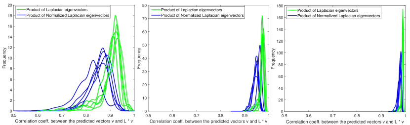
Figure 2: Smoothed probability density functions of vector correlation coefficients between $w_{i}^{S_{1}}\otimes w_{j}^{S_{2}}$ and $L_{S_{1}\otimes S_{2}}(w_{i}^{S_{1}}\otimes w_{j}^{S_{2}})$ are represented by using a green solid line, while between $v_{i}^{S_{1}}\otimes v_{j}^{S_{2}}$ and $L_{S_{1}\otimes S_{2}}(v_{i}^{S_{1}}\otimes v_{j}^{S_{2}})$ are represented using a blue solid line. Probability density functions are drawn for each of the edge density level 10%, 30% and 65%, respectively, for the Erdős-Rényi random graphs with 50 and 30 vertices.

3.1.2 Theoretical results for eigenvectors estimation

Given the performed experiments it can be noticed that some of the values of correlation coefficients that correspond to the approximation vectors $w_{i}^{S_{1}}\otimes w_{j}^{S_{2}}$ are mutually equal. Indeed, we can explicitly determine the values of correlation coefficients related to the vectors $w_{1}^{S_{1}}\otimes w_{j}^{S_{2}}$ and $w_{i}^{S_{1}}\otimes w_{1}^{S_{2}}$, for $2\leq j\leq n_{2}$ and $2\leq i\leq n_{1}$, and show that they do not depend on the vectors $w_{j}^{S_{2}}$ and $w_{i}^{S_{1}}$. In the following text, we prove that the correlation coefficients related to the vectors $w_{1}^{S_{1}}\otimes w_{j}^{S_{2}}$ and $w_{i}^{S_{1}}\otimes w_{1}^{S_{2}}$ only depend on the vertex degrees of $S_{1}$ and $S_{2}$, respectively.

Theorem 1

The correlation coefficients $r_{1,j}$ ($2\leq j\leq n_{2}$) corresponding to the vectors $L_{S_{1}\otimes S_{2}}(1_{S_{1}}\otimes w_{j}^{S_{2}})$ and $1_{S_{1}}\otimes w_{j}^{S_{2}}$ are equal to

$$\frac{\frac{d_{1}^{S_{1}}+\cdots+d_{n_{1}}^{S_{1}}}{n_{1}}}{\sqrt{\frac{{d_{1}^{S_{1}}}^{2}+\cdots+{d_{n_{1}}^{S_{1}}}^{2}}{n_{1}}}}.$$

Proof. Using the fact that $D_{S_{1}}1_{S_{1}}=A_{S_{1}}1_{S_{1}}=[d_{1}^{S_{1}},\ldots,d_{n_{1}}^{S_{1}}]^{T}$, we show that the vectors $L_{S_{1}\otimes S_{2}}(w_{1}^{S_{1}}\otimes w_{j}^{S_{2}})$ and $[d_{1}^{S_{1}},\ldots,d_{n_{1}}^{S_{1}}]^{T}\otimes w_{j}^{S_{2}}$ are colinear

$$L_{S_{1}\otimes S_{2}}(1_{S_{1}}\otimes w_{j}^{S_{2}}) = (D_{S_{1}}\otimes D_{S_{2}}-A_{S_{1}}\otimes A_{S_{2}})(1_{S_{1}}\otimes w_{j}^{S_{2}})$$ (6)

$$= (D_{S_{1}}1_{S_{1}})\otimes(D_{S_{2}}w_{j}^{S_{2}})-(A_{S_{1}}1_{S_{1}})\otimes(A_{S_{2}}w_{j}^{S_{2}})$$

$$= [d_{1}^{S_{1}},\ldots,d_{n_{1}}^{S_{1}}]^{T}\otimes(D_{S_{2}}-A_{S_{2}})w_{j}^{S_{2}}$$

$$= \mu_{j}^{S_{2}}[d_{1}^{S_{1}},\ldots,d_{n_{1}}^{S_{1}}]^{T}\otimes w_{j}^{S_{2}}.$$

According to (6) we have the following chain of equalities

$$r_{1,j} = \frac{\langle L_{S_{1}\otimes S_{2}}(1_{S_{1}}\otimes w_{j}^{S_{2}}),1_{S_{1}}\otimes w_{j}^{S_{2}}\rangle}{\|\mu_{j}^{S_{2}}[d_{1}^{S_{1}},\ldots,d_{n_{1}}^{S_{1}}]^{T}\otimes w_{j}^{S_{2}}\|\cdot\|1_{S_{1}}\otimes w_{j}^{S_{2}}\|}$$

$$= \frac{(\mu_{j}^{S_{2}}[d_{1}^{S_{1}},\ldots,d_{n_{1}}^{S_{1}}]\otimes{w_{j}^{S_{2}}}^{T})\cdot(1_{S_{1}}\otimes w_{j}^{S_{2}})}{\mu_{j}^{S_{2}}\|[d_{1}^{S_{1}},\ldots,d_{n_{1}}^{S_{1}}]\|\cdot\|1_{S_{1}}\|\cdot\|w_{j}^{S_{2}}\|^{2}}$$

$$= \frac{(\mu_{j}^{S_{2}}[d_{1}^{S_{1}},\ldots,d_{n_{1}}^{S_{1}}]1_{S_{1}})\otimes\|w_{j}^{S_{2}}\|^{2}}{\mu_{j}^{S_{2}}\sqrt{n_{1}}\|[d_{1}^{S_{1}},\ldots,d_{n_{1}}^{S_{1}}]\|\cdot\|w_{j}^{S_{2}}\|^{2}}$$

$$= \frac{\frac{d_{1}^{S_{1}}+\cdots+d_{n_{1}}^{S_{1}}}{n_{1}}}{\sqrt{\frac{{d_{1}^{S_{1}}}^{2}+\cdots+{d_{n_{1}}^{S_{1}}}^{2}}{n_{1}}}}.$$

$\square$

We see that $r_{1,j}=1$ if and only if the arithmetic mean of the vertex degrees of $S_{1}$ is equal to the root mean square of the same elements and it is well-known that it is true if and only if $S_{1}$ is a regular graph. On the other hand, the values of $r_{1,j}$ can be very low in the cases where there is a large gap between the lowest and highest vertex degrees in the graphic sequence of $S_{1}$, $1\leq d_{1}^{S_{1}}\leq\ldots\leq d_{n_{1}}^{S_{1}}\leq n_{1}-1$. For example, considering the complete bipartite graph $S_{1}=K_{1,n_{1}-1}$ and calculating the arithmetic mean and the root mean square of the vertex degrees which are $\frac{2n_{1}-2}{n_{1}}$ and $\sqrt{n_{1}-1}$, respectively, we can deduce that $r_{1,j}=\frac{2\sqrt{n_{1}-1}}{n_{1}}\rightarrow 0$, when $n_{1}\rightarrow\infty$. However, if the sizes of the partition sets in a bipartite graph become more equal (tend to $n_{1}/2$) then the coefficient $r_{1,j}\rightarrow 1$ (for the illustration we can take $S_{1}=K_{2,n_{1}-2}$ and obtain that $r_{1,j}=\frac{2\sqrt{2n_{1}-4}}{n_{1}}>\frac{2\sqrt{n_{1}-1}}{n_{1}}$). In addition, it can be noticed that the correlation coefficients do not decrease with the increase in the number of different vertex degrees in $S_{1}$. Indeed, if we consider the graph $S_{1}$ with an even order $n_{1}=2k+2$ and the graphic sequence $1,2,\ldots,k,k+1,k+1,k+2,\ldots,2k+1$, it can be determined that the arithmetic mean and the root mean square are $k+1$ and $\sqrt{\frac{(2k+1)(4k+3)+3(k+1)}{6}}$, respectively. Therefore, in this case we obtain high correlation coefficients $r_{1,j}=\frac{1}{\sqrt{\frac{4}{3}-\frac{1}{2(k+1)}+\frac{1}{6(k+1)^{2}}}}\rightarrow\frac{\sqrt{3}}{2}$, $k\rightarrow\infty$.

However, since we have obtained correlation coefficients $r_{1,j}$ using a certain number of synthetic networks produced by the Erdős-Rényi model, in the following text we theoretically discuss about the expected values of the correlation coefficients $r_{1,j}$, using the following auxiliary result.

Proposition 1 ([23] pp. 211)

Suppose that $X_{n}$ is $AN(\mu,c_{n}^{2}\Sigma)$ where $\Sigma$ is a symmetric nonnegative definite matrix and $c_{n}\rightarrow 0$ as $n\rightarrow\infty$. If $g(X)=(g_{1}(X),\ldots,g_{m}(X))^{\prime}$ is a mapping from $R^{k}$ into $R^{m}$ such that each $g_{i}$ is continuously differentiable in a neighborhood of $\mu$, and if $D\Sigma D^{\prime}$ has all of its diagonal elements non-zero, where $D$ is the $m\times k$ matrix $[(\frac{\partial g_{i}}{\partial x_{j}})(\mu)]$, then

$$g(X_{n}){\mbox{\ }is\ }AN(g(\mu),c_{n}^{2}D\Sigma D^{\prime}).$$

Theorem 2

If $S_{1}$ is Erdős-Rényi graph model, then the expected value of the correlation coefficient $r_{1,j}$ corresponding to the vectors $L_{S_{1}\otimes S_{2}}(1_{S_{1}}\otimes w_{j}^{S_{2}})$ and $1_{S_{1}}\otimes w_{j}^{S_{2}}$ tends to

$$\sqrt{\frac{(n_{1}-1)p}{1-p+(n_{1}-1)p}},$$ (7)

as $n_{1}\rightarrow\infty$.

Proof. Since the distribution of the degree of any particular vertex of the Erdős-Rényi graph $S_{1}=G(n_{1},p)$ is binomial, that is $P(d_{i}^{S_{1}}=k)={{n_{1}-1}\choose k}p^{k}(1-p)^{n_{1}-k-1}$, and the fact that the expected value of any vertex degree is equal to the expected value of the arithmetic mean of degrees $Y_{1}=\frac{d_{1}^{S_{1}}+\ldots+d_{n_{1}}^{S_{1}}}{n_{1}}$, we conclude that $E(Y_{1})=(n_{1}-1)p$ . Furthermore, as $n_{1}\rightarrow\infty$, according to the central limit theorem $Y_{1}$ has asymptotic normal distribution $AN(\mu_{1},\frac{\sigma_{1}^{2}}{n_{1}})$, where $\mu_{1}=E(Y_{1})$ and $\sigma_{1}^{2}=D(d_{i}^{S_{1}})=(n_{1}-1)p(1-p)$ ($E$ and $D$ are usual notation for expected value and dispersion, respectively). Similarly, as ${d_{i}^{S_{1}}}^{2}$, $1\leq i\leq n_{1}$, have the same distribution, we deduce that $Y_{2}=\frac{{d_{1}^{S_{1}}}^{2}+\cdots+{d_{n_{1}}^{S_{1}}}^{2}}{n_{1}}$ has asymptotic normal distribution $AN(\mu_{2},\frac{\sigma_{2}^{2}}{n_{1}})$, where $\mu_{2}=E(Y_{2})=E({d_{i}^{S_{1}}}^{2})$ and $\sigma_{2}^{2}=D({d_{i}^{S_{1}}}^{2})$. On the other hand, given that $E({d_{i}^{S_{1}}}^{2})=D(d_{i}^{S_{1}})+E({d_{i}^{S_{1}}})^{2}$ , we have that $\mu_{2}=(n_{1}-1)p(1-p)+(n_{1}-1)^{2}p^{2}$. Considering the two dimensional variable $X_{2}=[Y_{1},Y_{2}]$ it can be concluded that its asymptotic normal distribution is $AN([\mu_{1},\mu_{2}]^{\prime},c_{n}^{2}\Sigma)$, where $\Sigma$ represents a nonnegative definite symmetric matrix. Define $g(y_{1},y_{2})=\frac{y_{1}}{\sqrt{y_{2}}}$ which is a continuously differentiable function. Finally, using Proposition 1 we conclude that $g(X_{2})$ has asymptotic normal distribution $AN(\mu_{3},c_{n}^{2}D\Sigma D^{\prime})$, where $\mu_{3}=g(\mu_{1},\mu_{2})=\frac{\mu_{1}}{\sqrt{\mu_{2}}}$. Therefore, the expected value of the coefficient correlation $r_{1,j}$ is equal to $E(g(X_{2}))$ (according to Theorem 1) which tends to $\mu_{3}=\sqrt{\frac{(n_{1}-1)p}{1-p+(n_{1}-1)p}}$, as $n_{1}\rightarrow\infty$. $\square$

If we rewrite (7) in the form $\sqrt{\frac{1}{\frac{1-p}{(n_{1}-1)p}+1}}$, we conclude that the expected value of $r_{1,j}$ tends to $1$ when the order of the graph increases, for the fixed edge density $p$. Therefore, we show that $w_{1}^{S_{1}}\otimes w_{j}^{S_{2}}$, $2\leq j\leq n_{2}$, becomes a more stable approximation for the larger orders of graphs with constant edge level. Moreover, we report higher coefficient correlations $r_{i,j}$ when the order of graphs are $50$ and $100$, respectively (see Fig. 3). The same conclusion can be obtained if the order of graphs are $100$ and $200$, respectively.

Similarly, for a given order $n_{1}$ of the graph $S_{1}$, by rewriting (7) in the form $\sqrt{\frac{n_{1}-1}{\frac{1}{p}-1+(n_{1}-1)}}$, we conclude that $r_{1,j}\rightarrow 1$, if $p$ tends to $1$ and $r_{1,j}\rightarrow 0$, if $p$ tends to $0$. Notice that we have already obtained a more general conclusion by performing three types of experiments in which the correlation coefficients increase in total as long as the edge density increases (for a fixed $n_{1}$). In our experimental setup $p$ can not tend to $0$ since we deal with connected graphs. Namely, a sharp threshold for the connectedness of $S_{1}$ is $\frac{\ln n_{1}}{n_{1}}$ (more precisely if $p>\frac{(1+\epsilon)\ln n_{1}}{n_{1}}$ then the graph $S_{1}$ will almost surely be connected). Since the parameters in the experimental setup satisfy the mentioned condition, we almost surely deal with connected graphs and after applying the condition we obtain $r_{1,j}\geq\frac{1-\frac{1}{n_{1}}}{\frac{1}{(1+\epsilon)\ln n_{1}}+(1-\frac{2}{n_{1}})}$. Therefore, $r_{1,j}\rightarrow 1$, as $n_{1}\rightarrow\infty$, which theoretically confirms our experimental results that the correlation coefficient $r_{1,j}$ grows as long as the order of the connected Erdős-Rényi graph grows.

Figure 3: Smoothed probability density functions of vector correlation coefficients between $w_{i}^{S_{1}}\otimes w_{j}^{S_{2}}$ and $L_{S_{1}\otimes S_{2}}(w_{i}^{S_{1}}\otimes w_{j}^{S_{2}})$ are represented by using a solid green line, while between $v_{i}^{S_{1}}\otimes v_{j}^{S_{2}}$ and $L_{S_{1}\otimes S_{2}}(v_{i}^{S_{1}}\otimes v_{j}^{S_{2}})$ are represented using a solid blue line. Probability density functions are drawn for the edge density level of 10%, for the Erdős-Rényi random graphs with 50 and 100 vertices.

In the following text, we estimate the correlation coefficients related to the vectors $v_{1}^{S_{1}}\otimes v_{j}^{S_{2}}$ and $v_{i}^{S_{1}}\otimes v_{1}^{S_{2}}$ in terms of the vertex degrees of $S_{1}$ and $S_{2}$, respectively. Moreover, we prove that the expected values of these coefficients $r^{\prime}_{1,j}$ can exceed the expected value of $r_{1,j}$ given by (7), when $n_{1}\rightarrow\infty$ and $n_{2}\rightarrow\infty$.

Lemma 1

The scalar product of the vectors $L_{S_{1}\otimes S_{2}}(v_{1}^{S_{1}}\otimes v_{j}^{S_{2}})$ and $v_{1}^{S_{1}}\otimes v_{j}^{S_{2}}$ is greater than or equal to

$$({d_{1}^{S_{1}}}^{2}+\cdots+{d_{n_{1}}^{S_{1}}}^{2})\ \ {v_{j}^{S_{2}}}^{T}L_{S_{2}}v_{j}^{S_{2}},$$

for $1\leq j\leq n_{2}$. The equality holds true if and only if $S_{1}$ is regular.

Proof. Since $v_{1}^{S_{1}}=D_{S_{1}}^{\frac{1}{2}}1_{S_{1}}$ we have the following chain of equalities

$$\langle L_{S_{1}\otimes S_{2}}(D_{S_{1}}^{\frac{1}{2}}1_{S_{1}}\otimes v_{j}^{S_{2}}),D_{S_{1}}^{\frac{1}{2}}1_{S_{1}}\otimes v_{j}^{S_{2}}\rangle=(D_{S_{1}}^{\frac{1}{2}}1_{S_{1}}\otimes v_{j}^{S_{2}})^{T}L_{S_{1}\otimes S_{2}}(D_{S_{1}}^{\frac{1}{2}}1_{S_{1}}\otimes v_{j}^{S_{2}})$$ (8)

$$= (D_{S_{1}}^{\frac{1}{2}}1_{S_{1}}\otimes v_{j}^{S_{2}})^{T}(D_{S_{1}}\otimes D_{S_{2}}-A_{S_{1}}\otimes A_{S_{2}})(D_{S_{1}}^{\frac{1}{2}}1_{S_{1}}\otimes v_{j}^{S_{2}})$$

$$= (1_{S_{1}}^{T}D_{S_{1}}^{\frac{1}{2}}\otimes{v_{j}^{S_{2}}}^{T})(D_{S_{1}}\otimes D_{S_{2}})(D_{S_{1}}^{\frac{1}{2}}1_{S_{1}}\otimes v_{j}^{S_{2}})-(1_{S_{1}}^{T}D_{S_{1}}^{\frac{1}{2}}\otimes{v_{j}^{S_{2}}}^{T})(A_{S_{1}}\otimes A_{S_{2}})(D_{S_{1}}^{\frac{1}{2}}1_{S_{1}}\otimes v_{j}^{S_{2}})$$

$$= (1_{S_{1}}^{T}D_{S_{1}}^{\frac{1}{2}}D_{S_{1}}D_{S_{1}}^{\frac{1}{2}}1_{S_{1}})\otimes({v_{j}^{S_{2}}}^{T}D_{S_{2}}v_{j}^{S_{2}})-(1_{S_{1}}^{T}D_{S_{1}}^{\frac{1}{2}}A_{S_{1}}D_{S_{1}}^{\frac{1}{2}}1_{S_{1}})\otimes({v_{j}^{S_{2}}}^{T}A_{S_{2}}v_{j}^{S_{2}})$$

$$= (1_{S_{1}}^{T}D_{S_{1}}^{2}1_{S_{1}})\otimes({v_{j}^{S_{2}}}^{T}D_{S_{2}}v_{j}^{S_{2}})-([{d_{1}^{S_{1}}}^{\frac{1}{2}},\ldots,{d_{n_{1}}^{S_{1}}}^{\frac{1}{2}}]A_{S_{1}}[{d_{1}^{S_{1}}}^{\frac{1}{2}},\ldots,{d_{n_{1}}^{S_{1}}}^{\frac{1}{2}}]^{T})\otimes({v_{j}^{S_{2}}}^{T}A_{S_{2}}v_{j}^{S_{2}}).$$

Furthermore, the quadratic forms $1_{S_{1}}^{T}D_{S_{1}}^{2}1_{S_{1}}$ and $[{d_{1}^{S_{1}}}^{\frac{1}{2}},\ldots,{d_{n_{1}}^{S_{1}}}^{\frac{1}{2}}]A_{S_{1}}[{d_{1}^{S_{1}}}^{\frac{1}{2}},\ldots,{d_{n_{1}}^{S_{1}}}^{\frac{1}{2}}]^{T}$ are equal to $\sum_{i=1}^{n_{1}}{d_{i}^{S_{1}}}^{2}$ and $\sum_{\{i,j\}\in E(S_{1})}2{d_{i}^{S_{1}}}^{\frac{1}{2}}{d_{j}^{S_{1}}}^{\frac{1}{2}}$, respectively. According to the inequality of arithmetic and geometric means it holds that $\sum_{\{i,j\}\in E(S_{1})}2{d_{i}^{S_{1}}}^{\frac{1}{2}}{d_{j}^{S_{1}}}^{\frac{1}{2}}\leq\sum_{\{i,j\}\in E(S_{1})}{d_{i}}^{S_{1}}+{d_{j}}^{S_{1}}=\sum_{i=1}^{n_{1}}{d_{i}^{S_{1}}}^{2}$. The equality holds true if and only if $d_{1}^{S_{1}}=\ldots=d_{n_{1}}^{S_{1}}$. Finally, we have that the term (8) is greater than or equal to $\sum_{i=1}^{n_{1}}{d_{i}^{S_{1}}}^{2}({v_{j}^{S_{2}}}^{T}D_{S_{2}}v_{j}^{S_{2}})-\sum_{i=1}^{n_{1}}{d_{i}^{S_{1}}}^{2}({v_{j}^{S_{2}}}^{T}A_{S_{2}}v_{j}^{S_{2}})=\sum_{i=1}^{n_{1}}{d_{i}^{S_{1}}}^{2}({v_{j}^{S_{2}}}^{T}L_{S_{2}}v_{j}^{S_{2}})$. $\square$

Lemma 2

The norm of the vector $L_{S_{1}\otimes S_{2}}(v_{1}^{S_{1}}\otimes v_{j}^{S_{2}})$ is less than or equal to

$$\sqrt{{d_{1}^{S_{1}}}^{3}+\cdots{d_{n_{1}}^{S_{1}}}^{3}}\ \|L_{S_{2}}v_{j}^{S_{2}}\|,$$

for $1\leq j\leq n_{2}$. The equality holds true if and only if $S_{1}$ is regular.

Proof. We have the following chain of equalities

$$L_{S_{1}\otimes S_{2}}(D_{S_{1}}^{\frac{1}{2}}1_{S_{1}}\otimes v_{j}^{S_{2}})=(D_{S_{1}}\otimes D_{S_{2}}-A_{S_{1}}\otimes A_{S_{2}})(D_{S_{1}}^{\frac{1}{2}}1_{S_{1}}\otimes v_{j}^{S_{2}})$$

$$= (D_{S_{1}}D_{S_{1}}^{\frac{1}{2}}1_{S_{1}})\otimes(D_{S_{2}}v_{j}^{S_{2}})-(A_{S_{1}}D_{S_{1}}^{\frac{1}{2}}1_{S_{1}})\otimes(A_{S_{2}}v_{j}^{S_{2}})$$

$$= [{d_{1}^{S_{1}}}^{\frac{3}{2}},\ldots,{d_{n_{1}}^{S_{1}}}^{\frac{3}{2}}]^{T}\otimes(D_{S_{2}}v_{j}^{S_{2}})-[\sum_{\{1,i\}\in E(S_{1})}d_{i}^{\frac{1}{2}},\ldots,\sum_{\{n_{1},i\}\in E(S_{1})}d_{i}^{\frac{1}{2}}]^{T}\otimes(A_{S_{2}}v_{j}^{S_{2}}).$$

Furthermore, since $u\otimes(Av)=(u\otimes A)v$, where $u^{T}\in R^{n_{1}}$, $v^{T}\in R^{n_{2}}$ and $A\in R^{n_{2}\times n_{2}}$ it holds that

$$\|L_{S_{1}\otimes S_{2}}(D_{S_{1}}^{\frac{1}{2}}1_{S_{1}}\otimes v_{j}^{S_{2}})\| =$$

$$=\|([{d_{1}^{S_{1}}}^{\frac{3}{2}},\ldots,{d_{n_{1}}^{S_{1}}}^{\frac{3}{2}}]^{T}\otimes D_{S_{2}}-[\sum_{\{1,i\}\in E(S_{1})}d_{i}^{\frac{1}{2}},\ldots,\sum_{\{n_{1},i\}\in E(S_{1})}d_{i}^{\frac{1}{2}}]^{T}\otimes A_{S_{2}})v_{j}^{S_{2}}\|.$$

Now, if we denote $B=[{d_{1}^{S_{1}}}^{\frac{3}{2}},\ldots,{d_{n_{1}}^{S_{1}}}^{\frac{3}{2}}]^{T}\otimes D_{S_{2}}-[\sum_{\{1,i\}\in E(S_{1})}{d_{i}^{S_{1}}}^{\frac{1}{2}},\ldots,\sum_{\{n_{1},i\}\in E(S_{1})}{d_{i}^{S_{1}}}^{\frac{1}{2}}]^{T}\otimes A_{S_{2}}$ and $A_{S_{2}}=[a_{i,j}]$, $1\leq i,j\leq n_{2}$, then we can easily conclude that

$$B=\begin{bmatrix}B_{1}\\ B_{2}\\ \vdots\\ B_{n_{1}}\end{bmatrix},\quad B_{k}=\left\{\begin{aligned} &{d_{k}^{S_{1}}}^{\frac{3}{2}}d_{i}^{S_{2}},&&\text{if}\ i=j\\ &-\sum_{\{k,l\}\in E(S_{1})}{d_{l}^{S_{1}}}^{\frac{1}{2}}a_{i,j},&&\text{if}\ i\neq j\end{aligned}\right.,\quad 1\leq k\leq n_{1}.$$

Therefore, we obtain that

$$\begin{array}[]{lcl}\|Bv_{j}^{S_{2}}\|&=&\|[{d_{1}^{S_{1}}}^{\frac{3}{2}},\ldots,{d_{n_{1}}^{S_{1}}}^{\frac{3}{2}}]^{T}\otimes(D_{S_{2}}v_{j}^{S_{2}})\|+\|[\displaystyle\sum_{\{1,i\}\in E(S_{1})}{d_{i}^{S_{1}}}^{\frac{1}{2}},\ldots,\sum_{\{n_{1},i\}\in E(S_{1})}{d_{i}^{S_{1}}}^{\frac{1}{2}}]^{T}\otimes(-A_{S_{2}}v_{j}^{S_{2}})\|\\ &\leq&\|[{d_{1}^{S_{1}}}^{\frac{3}{2}},\ldots,{d_{n_{1}}^{S_{1}}}^{\frac{3}{2}}]^{T}\|\otimes\|D_{S_{2}}v_{j}^{S_{2}}\|+\|[\displaystyle\sum_{\{1,i\}\in E(S_{1})}{d_{i}^{S_{1}}}^{\frac{1}{2}},\ldots,\sum_{\{n_{1},i\}\in E(S_{1})}{d_{i}^{S_{1}}}^{\frac{1}{2}}]^{T}\|\otimes\|(A_{S_{2}}v_{j}^{S_{2}})\|.\\ \end{array}$$ (10)

Furthermore, according to the inequality between the arithmetic mean and root mean square
$(\sum_{\{k,i\}\in E(S_{1})}{d_{i}^{S_{1}}}^{\frac{1}{2}})^{2}\leq{d_{k}^{S_{1}}}\sum_{\{k,i\}\in E(S_{1})}{d_{i}^{S_{1}}}$, for $1\leq k\leq n_{1}$, the following inequalities holds

$$\|[\sum_{\{1,i\}\in E(S_{1})}{d_{i}^{S_{1}}}^{\frac{1}{2}},\ldots,\sum_{\{n_{1},i\}\in E(S_{1})}{d_{i}^{S_{1}}}^{\frac{1}{2}}]^{T}\|^{2} \leq 2\sum_{\{i,j\}\in E(S_{1})}{d_{i}^{S_{1}}}{d_{j}^{S_{1}}}$$

$$\leq \sum_{\{i,j\}\in E(S_{1})}{d_{i}^{S_{1}}}^{2}+{d_{j}^{S_{1}}}^{2}=\sum_{i=1}^{n_{1}}{d_{i}^{S_{1}}}^{3}=\|[{d_{1}^{S_{1}}}^{\frac{3}{2}},\ldots,{d_{n_{1}}^{S_{1}}}^{\frac{3}{2}}]^{T}\|^{2}.$$

The equality holds true if and only if $d_{1}^{S_{1}}=\ldots=d_{n_{1}}^{S_{1}}$. Now, according to the inequalities (3.1.2), (10) and (3.1.2) we conclude that

$$\|L_{S_{1}\otimes S_{2}}(D_{S_{1}}^{\frac{1}{2}}1_{S_{1}}\otimes v_{j}^{S_{2}})\|=\|Bv_{j}^{S_{2}}\|\leq\sum_{i=1}^{n_{1}}\sqrt{{d_{i}^{S_{1}}}^{3}}(\|D_{S_{2}}v_{j}^{S_{2}}\|+\|A_{S_{2}}v_{j}^{S_{2}}\|).$$

From the fact that $\|L_{S_{2}}v_{j}^{S_{2}}\|=\|(D_{S_{2}}-A_{S_{2}})v_{j}^{S_{2}}\|=\|D_{S_{2}}v_{j}^{S_{2}}\|+\|A_{S_{2}}v_{j}^{S_{2}}\|$ we finally have that

$$\|L_{S_{1}\otimes S_{2}}(D_{S_{1}}^{\frac{1}{2}}1_{S_{1}}\otimes v_{j}^{S_{2}})\|\leq\sqrt{\sum_{i=1}^{n_{1}}{d_{i}^{S_{1}}}^{3}}\|L_{S_{2}}v_{j}^{S_{2}}\|.$$

$\square$

Theorem 3

The correlation coefficients $r^{\prime}_{1,j}$ ($2\leq j\leq n_{2}$) corresponding to the vectors $L_{S_{1}\otimes S_{2}}(D_{S_{1}}^{\frac{1}{2}}1_{S_{1}}\otimes v_{j}^{S_{2}})$ and $D_{S_{1}}^{\frac{1}{2}}1_{S_{1}}\otimes v_{j}^{S_{2}}$ are greater than or equal to

$$\frac{{d_{1}^{S_{1}}}^{2}+\cdots+{d_{n_{1}}^{S_{1}}}^{2}}{\sqrt{({d_{1}^{S_{1}}}^{3}+\cdots+{d_{n_{1}}^{S_{1}}}^{3})({d_{1}^{S_{1}}}+\cdots+{d_{n_{1}}^{S_{1}}})}}r_{j}^{S_{2}},$$

where $r_{j}^{S_{2}}$ is the correlation coefficient corresponding to the vectors $L_{S_{2}}v_{j}^{S_{2}}$ and $v_{j}^{S_{2}}$.

Proof. According to Lemma 1 and Lemma 2 we obtain that

$$r^{\prime}_{1,j} = \frac{\langle L_{S_{1}\otimes S_{2}}(D_{S_{1}}^{\frac{1}{2}}1_{S_{1}}\otimes v_{j}^{S_{2}}),D_{S_{1}}^{\frac{1}{2}}1_{S_{1}}\otimes v_{j}^{S_{2}}\rangle}{\|L_{S_{1}\otimes S_{2}}(D_{S_{1}}^{\frac{1}{2}}1_{S_{1}}\otimes v_{j}^{S_{2}})\|\cdot\|D_{S_{1}}^{\frac{1}{2}}1_{S_{1}}\otimes v_{j}^{S_{2}}\|}$$

$$\geq \frac{({d_{1}^{S_{1}}}^{2}+\cdots+{d_{n_{1}}^{S_{1}}}^{2})\ \ {v_{j}^{S_{2}}}^{T}L_{S_{2}}v_{j}^{S_{2}}}{\sqrt{{d_{1}^{S_{1}}}^{3}+\cdots{d_{n_{1}}^{S_{1}}}^{3}}\ \|L_{S_{2}}v_{j}^{S_{2}}\|\sqrt{d_{1}^{S_{1}}+\cdots d_{n_{1}}^{S_{1}}}\|v_{j}^{S_{2}}\|}$$

$$= \frac{{d_{1}^{S_{1}}}^{2}+\cdots+{d_{n_{1}}^{S_{1}}}^{2}}{\sqrt{{d_{1}^{S_{1}}}^{3}+\cdots{d_{n_{1}}^{S_{1}}}^{3}}\ \sqrt{d_{1}^{S_{1}}+\cdots d_{n_{1}}^{S_{1}}}}\cdot\frac{{v_{j}^{S_{2}}}^{T}L_{S_{2}}v_{j}^{S_{2}}}{\|L_{S_{2}}v_{j}^{S_{2}}\|\|v_{j}^{S_{2}}\|}.$$

$\square$

Let us mention that the sum of cubes of vertex degrees of a graph $G$ is known as the forgotten topological index denoted by $F(G)$ [24], while the sum of squares of vertex degrees of a graph $G$ represents well known first Zagreb index, denoted by $M_{1}^{1}(G)$ [25]. In the following statement we actually prove that the expected value of $\frac{M_{1}^{1}(G)}{\sqrt{2mF(t)}}$ is greater than or equal to the expected value of correlation coefficient $r_{1,j}$ for the random graphs in the asymptotic case. However, it can be shown that $\frac{M_{1}^{1}(G)}{\sqrt{2mF(t)}}\geq r_{1,j}$ does not always hold for an arbitrary graph and it would be nice to find the minimum of the function $\frac{M_{1}^{1}(G)}{\sqrt{2mF(t)}r_{1,j}}$. This would make a more elegant expression for the upper bound for $F(G)$ than those that can be found in the literature [26].

Theorem 4

The asymptotic value of the expected value of the correlation coefficient $r_{1,j}$ is less than or equal to the asymptotic value of the expected value of

$$\frac{{d_{1}^{S_{1}}}^{2}+\cdots+{d_{n_{1}}^{S_{1}}}^{2}}{\sqrt{({d_{1}^{S_{1}}}^{3}+\cdots+{d_{n_{1}}^{S_{1}}}^{3})({d_{1}^{S_{1}}}+\cdots+{d_{n_{1}}^{S_{1}}})}},$$

as $n_{1}\rightarrow\infty$.

Proof. According to Theorem 2 we have that the asymptotic value of expected value of the correlation coefficient $r_{1,j}$ is equal to $\sqrt{\frac{(n_{1}-1)p}{1-p+(n_{1}-1)p}}$, as $n_{1}\rightarrow\infty$. On the other hand, as $P(d_{i}^{S_{1}}=k)={{n_{1}-1}\choose k}p^{k}(1-p)^{n_{1}-k-1}$ we have that $E(Y_{1})=n_{1}(n_{1}-1)p$ for $Y_{1}=d_{1}^{S_{1}}+\ldots+d_{n_{1}}^{S_{1}}$. Similarly, we can conclude that $E(Y_{2})=n_{1}((n_{1}-1)p(1-p)+(n_{1}-1)^{2}p^{2})$ for $Y_{2}={d_{1}^{S_{1}}}^{2}+\cdots+{d_{n_{1}}^{S_{1}}}^{2}$ and $E(Y_{3})=n_{1}((n_{1}-1)(n_{1}-2)(n_{1}-3)p^{3}+3p^{2}(n_{1}-1)(n_{1}-2)+(n_{1}-1)p)$ for $Y_{3}={d_{1}^{S_{1}}}^{3}+\cdots+{d_{n_{1}}^{S_{1}}}^{3}$. Using Proposition 1 we can conduct the similar proof as we do in Theorem 2 and conclude that that asymptotic value of the expected value of $\frac{{d_{1}^{S_{1}}}^{2}+\cdots+{d_{n_{1}}^{S_{1}}}^{2}}{\sqrt{({d_{1}^{S_{1}}}^{3}+\cdots+{d_{n_{1}}^{S_{1}}}^{3})({d_{1}^{S_{1}}}+\cdots+{d_{n_{1}}^{S_{1}}})}},$ as $n_{1}\rightarrow\infty$, is equal to $\frac{E(Y_{2})}{\sqrt{E(Y_{1})E(Y_{3})}}$. It only remains to show that

$$\frac{n_{1}((n_{1}-1)p(1-p)+(n_{1}-1)^{2}p^{2})}{\sqrt{n_{1}(n_{1}-1)p\ n_{1}((n_{1}-1)(n_{1}-2)(n_{1}-3)p^{3}+3p^{2}(n_{1}-1)(n_{1}-2)+(n_{1}-1)p)}}\geq\sqrt{\frac{(n_{1}-1)p}{1-p+(n_{1}-1)p}}.$$

After a short calculation, the inequality can be reduced to

$$\sqrt{\frac{(1-p+(n_{1}-1)p)^{3}}{(n_{1}-1)(n_{1}-2)(n_{1}-3)p^{3}+3(n_{1}-1)(n_{1}-2)p+(n_{1}-1)p}}\geq 1,$$

which is equivalent to $(n_{1}-2)p^{3}-3(n_{1}-2)p^{2}+(2n_{1}-5)p+1\geq 0$. Furthermore, this can be rewritten in the following way

$$n_{1}\geq 2+\frac{2p^{3}-6p^{2}+5p-1}{p^{3}-3p^{2}+2p}=2+\frac{p-1}{p^{3}-3p^{2}+2p}=2+\frac{p-1}{p(p-1)(p-2)}=2-\frac{1}{p(2-p)}.$$

The arithmetic-geometric mean inequality implies that $p(2-p)\leq(\frac{p+2-p}{2})^{2}=1$ and therefore we get $n_{1}\geq 1\geq 2-\frac{1}{p(2-p)}$, which is obviously true. $\square$

According to Theorem 3 and Theorem 4 we have the following chain of inequalities

$$E(r^{\prime}_{1,j})\geq E(\frac{{d_{1}^{S_{1}}}^{2}+\cdots+{d_{n_{1}}^{S_{1}}}^{2}}{\sqrt{({d_{1}^{S_{1}}}^{3}+\cdots+{d_{n_{1}}^{S_{1}}}^{3})({d_{1}^{S_{1}}}+\cdots+{d_{n_{1}}^{S_{1}}})}}r_{j}^{S_{2}})\geq E(r_{1,j})E(r_{j}^{S_{2}}),$$

as $n_{1}\rightarrow\infty$. Moreover, we see that the lower bound of $r^{\prime}_{1,j}$ depends on the degrees of $S_{1}$ and the correlation coefficient $r_{j}^{S_{2}}$, while $r_{1,j}$ depends only on the degrees of $S_{1}$. Therefore, for the higher values $r_{S_{2}}$ it will be more likely that the expected values of $r^{\prime}_{1,j}$ is greater than the expected values of $r_{1,j}$. In fact, if we choose $S_{2}$ to be the graph such that $r_{j}^{S_{2}}$ is close to $1$ (if $S_{2}$ is regular then $r_{j}^{S_{2}}=1$) we can conclude that $E(r^{\prime}_{1,j})\geq E(r_{1,j})$, for every $1\leq j\leq n_{2}$, as $n_{1}\rightarrow\infty$.

3.1.3 Experimental and theoretical results for eigenvalues estimation

Furthermore, we show the distributions of percentage errors in estimated Laplacian spectra of the Kronecker product of graphs compared to the actual spectrum. The error is calculated over one hundred independent tests for the Kronecker product of the Erdős-Rényi random graphs with 50 and 30 vertices. The errors for the estimated spectrum corresponding to the eigenvectors $w_{i}^{S_{1}}\otimes w_{j}^{S_{2}}$ are always drawn on the left hand side, while the errors for the estimated spectrum corresponding to the eigenvectors $v_{i}^{S_{1}}\otimes v_{j}^{S_{2}}$ are always drawn on the right hand side of Figure 4. Each row of the figure corresponds to one of the edge density levels of 10%, 30%, and 65%, respectively. The solid black curve shows the median, and the shaded areas show ranges from 5 to 95 percentiles. Notice that when the edge density increases, the percentage errors become smaller for both approximations. The characteristic shapes of error distributions for the estimated spectrum corresponding to the eigenvectors $w_{i}^{S_{1}}\otimes w_{j}^{S_{2}}$, seen in Figure 4 (left hand side) have sudden jumps at the beginning followed by a gradual decrease and they are fairly consistent across various network density levels that we tested. There is no a sudden jump at the beginning, for the estimated spectrum corresponding to the eigenvectors $v_{i}^{S_{1}}\otimes v_{j}^{S_{2}}$, but there is a small error widening for the largest eigenvalues. In the case of the estimated spectrum corresponding to the eigenvectors $w_{i}^{S_{1}}\otimes w_{j}^{S_{2}}$, the median takes positive values for the approximately first half of eigenvalues and negative values for the second half. In the case of the estimated spectrum corresponding to the eigenvectors $v_{i}^{S_{1}}\otimes v_{j}^{S_{2}}$, the distribution of percentage errors becomes more stable, that is, the median is almost a straight line with value 0 for every eigenvalue (right hand side of Figure 4). It could be seen that the error ranges are almost uniformly distributed around 0.

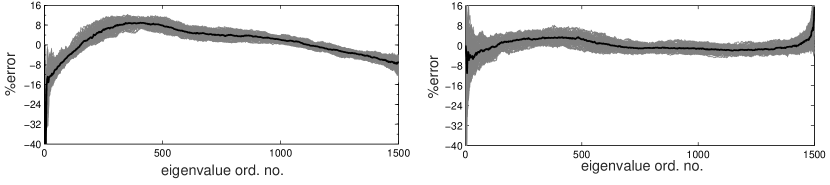
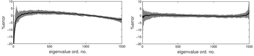
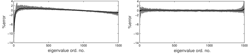
Figure 4: Distribution of percentage errors in estimated Laplacian spectra of the Kronecker product of Erdős-Rényi random graphs (50 and 30 vertices) compared to original ones. Left hand side is reserved for the spectrum of the vectors $w_{i}^{S_{1}}\otimes w_{j}^{S_{2}}$ and right hand side for the spectrum of the vectors $v_{i}^{S_{1}}\otimes v_{j}^{S_{2}}$. Rows correspond to the edge density levels of 10%, 30% and 65%.

Here we give a theoretical explanation of why the estimated eigenvalues corresponding to $v_{i}^{S_{1}}\otimes v_{j}^{S_{2}}$ for the random graphs become more accurate to the real expected values when the network grows or the edge density level increases. Conducted experiments show that this approximation produces reasonable estimation of Laplacian spectra with percentage errors confined within a $\pm$10%, $\pm$5% and $\pm$2% range for most eigenvalues when the edge density percentages are 10%, 30% and 65%, respectively. We use the following statement in order to show a theoretical justification for the above claim.

Theorem 5

[27] Let $G$ be a random graph, where $pr(v_{i}\sim v_{j})=p_{ij}$, and each edge is independent of each other edge. Let $A$ be the adjacency matrix of $G$, and $\bar{A}=E(A)$, so $\overline{A}_{ij}=p_{ij}$. Let $D$ be the diagonal matrix with $D_{ii}=deg(v_{i})$, and $\bar{D}=E(D)$. Let $\bar{\delta}=\bar{\delta}(G)$ be the minimum expected degree of $G$, and $\mathcal{L}$ the normalized Laplacian matrix for $G$. For any $\epsilon>0$, if there exists a constant $k=k(\epsilon)$ such that $\bar{\delta}>k\,ln\,n$, then with probability at least $1-\epsilon$, the $j$-th eigenvalues of $\mathcal{L}$ and $\bar{\mathcal{L}}$ satisfy

$$|\lambda_{j}(\mathcal{L})-\lambda_{j}(\bar{\mathcal{L}})|\leq 2\sqrt{\frac{3ln(\frac{4n}{\epsilon})}{\bar{\delta}}}$$

for all $1\leq j\leq n$, where $\bar{\mathcal{L}}=I-\bar{D}^{-\frac{1}{2}}\bar{A}\,\bar{D}^{-\frac{1}{2}}$.

Let $G_{n,p}$ be a random graph with order $n$ and probability of creation of an edge $p$. Since in the experiments we use the factor graphs with the same edge density percentage (denote these graphs by $G_{n_{1},p_{1}}$ and $G_{n_{2},p_{2}}$), without loss of generality, we may set $p_{1}=p_{2}=p$ (an identical analysis can be conducted when $p_{1}\neq p_{2}$). For the expected adjacency matrices of the random graphs $G_{n_{1},p}$ and $G_{n_{2},p}$ hold $\bar{A}_{n_{1}}=p(J_{n_{1}}-I_{n_{1}})$ and $\bar{A}_{n_{2}}=p(J_{n_{2}}-I_{n_{2}})$. By $A_{n_{1}}$ and $A_{n_{2}}$ we denote the adjacency matrices of $G_{n_{1},p_{1}}$ and $G_{n_{2},p_{2}}$. By $\mathcal{L}(G_{n_{1},p}\otimes G_{n_{2},p})$ we also denote the normalized Laplacian matrix for the graph $G_{n_{1},p}\otimes G_{n_{2},p}$.

First, we show that $\bar{\delta}=\bar{\delta}(G_{n_{1},p}\otimes G_{n_{2},p})\sim n_{1}n_{2}$. Notice also that since the sum of each row of the matrix $\bar{A}_{n_{1}}\otimes\bar{A}_{n_{2}}$ is equal to $p^{2}(n_{1}-1)(n_{2}-1)$, then it is clear that $\delta(\bar{G}_{n_{1},p}\otimes\bar{G}_{n_{2},p})=p^{2}(n_{1}-1)(n_{2}-1)$. Let $Z=\min\{d^{1}_{i}d^{2}_{k}\ |\ 1\leq i\leq n_{1}\ 1\leq k\leq n_{2}\}$, where $d_{i}^{1}$ and $d_{k}^{2}$ are the degrees of the vertices in $G_{n_{1},p_{1}}$ and $G_{n_{2},p}$, respectively. Therefore, we have that $\bar{\delta}=E(Z)$. According to Jensen’s inequality, it holds that $e^{-t\bar{\delta}}\leq E(e^{-tZ})$, for any positive real $t$. Furthermore, according to the definition of $Z$, we have the following chain of relation

$$e^{-t\bar{\delta}}\leq E(e^{-tZ})=E(e^{-t\min_{i,j}\{d^{1}_{i}d^{2}_{k}\}})=E(\max_{i,j}e^{-td^{1}_{i}d^{2}_{k}})\leq\sum_{i,j}E(e^{-td^{1}_{i}d^{2}_{k}})=n_{1}n_{2}E(e^{-td^{1}_{i}d^{2}_{k}}),$$ (12)

for any $1\leq i\leq n_{1}$ and $1\leq k\leq n_{2}$.

As $n_{1},n_{2}\rightarrow\infty$, according to the central limit theorem $d^{1}_{i}$ and $d^{2}_{k}$ have asymptotic normal distribution $AN(\mu_{1},\sigma_{1}^{2})$ and $AN(\mu_{2},\sigma_{2}^{2})$, respectively, where $\mu_{1}=n_{1}p$, $\mu_{2}=n_{2}p$, $\sigma_{1}=\sqrt{n_{1}pq}$ and $\sigma_{2}=\sqrt{n_{2}pq}$. Considering the two dimensional variable $X=[d^{1}_{i},d^{2}_{k}]$ it can be concluded that it has asymptotic normal distribution and since $g(x,y)=e^{-txy}$ is a continuously differentiable function we conclude that $g(X)$ has an asymptotic normal distribution. Therefore, when $n_{1},n_{2}\rightarrow\infty$, we have that $E(e^{-td^{1}_{i}d^{2}_{k}})=\frac{1}{2\pi\sigma_{1}\sigma_{2}}\int_{-\infty}^{\infty}\int_{-\infty}^{\infty}e^{-txy}e^{\frac{1}{2}(\frac{x-\mu_{1}}{\sigma_{1}})}e^{\frac{1}{2}(\frac{y-\mu_{2}}{\sigma_{2}})}dxdy$. After the substitutions $x\rightarrow\frac{x-\mu_{1}}{\sigma_{1}}$, $y\rightarrow\frac{y-\mu_{2}}{\sigma_{2}}$ and certain number of elementary algebraic transformations we obtain that

$$E(e^{-td^{1}_{i}d^{2}_{k}}) = \frac{e^{-t\mu_{1}\mu_{2}}}{2\pi}\int_{-\infty}^{\infty}e^{-t\mu_{1}\sigma_{2}y-\frac{y^{2}}{2}}e^{\frac{t^{2}\sigma_{1}^{2}(\mu_{2}+\sigma_{2}y)^{2}}{2}}\int_{-\infty}^{\infty}e^{\frac{(x+t\sigma_{1}(\mu_{2}+\sigma_{2}y))^{2}}{2}}dxdy$$

$$= \frac{e^{-t\mu_{1}\mu_{2}}}{\sqrt{2\pi}}\int_{-\infty}^{\infty}e^{-t\mu_{1}\sigma_{2}y-\frac{y^{2}}{2}+\frac{t^{2}\sigma_{1}^{2}(\mu_{2}+\sigma_{2}y)^{2}}{2}}dy.$$

The last integral can be rewritten in the following form $\frac{1}{\sqrt{2\pi}}e^{-t\mu_{1}\mu_{2}}e^{\frac{{t^{2}\sigma_{1}^{2}\mu_{2}^{2}}}{2}}\int_{-\infty}^{\infty}e^{\frac{-y^{2}A-2yB}{2}}$, where $A=1-t^{2}\sigma_{1}^{2}\sigma_{2}^{2}$ and $B=-t\mu_{1}\sigma_{2}+t^{2}\sigma_{1}^{2}\mu_{2}\sigma_{2}$. Finally, we have that

$$E(e^{-td^{1}_{i}d^{2}_{k}}) = \frac{1}{\sqrt{2\pi}}e^{-t\mu_{1}\mu_{2}+\frac{{t^{2}\sigma_{1}^{2}\mu_{2}^{2}}}{2}}e^{\frac{B^{2}}{2A}}\int_{-\infty}^{\infty}e^{\frac{-(\sqrt{A}(y-\frac{B}{A}))^{2}}{2}}dy=\frac{1}{\sqrt{2\pi}}e^{-t\mu_{1}\mu_{2}+\frac{{t^{2}\sigma_{1}^{2}\mu_{2}^{2}}}{2}+\frac{B^{2}}{2A}}\frac{\sqrt{2\pi}}{\sqrt{A}}$$

$$= \frac{e^{-t\mu_{1}\mu_{2}+\frac{{t^{2}\sigma_{1}^{2}\mu_{2}^{2}}}{2}+\frac{(-t\mu_{1}\sigma_{2}+t^{2}\sigma_{1}^{2}\mu_{2}\sigma_{2})^{2}}{2(1-t^{2}\sigma_{1}^{2}\sigma_{2}^{2})}}}{\sqrt{1-t^{2}\sigma_{1}^{2}\sigma_{2}^{2}}}$$

$$= \frac{e^{\frac{-2t\mu_{1}\mu_{2}+(\mu_{1}^{2}\sigma_{2}^{2}+\mu_{2}^{2}\sigma_{1}^{2})t^{2}}{2(1-t^{2}\sigma_{1}^{2}\sigma_{2}^{2})}}}{\sqrt{1-t^{2}\sigma_{1}^{2}\sigma_{2}^{2}}}.$$

According to (12) we obtain

$$\bar{\delta}\geq-\frac{ln(n_{1}n_{2})}{t}-\frac{-2\mu_{1}\mu_{2}+(\mu_{1}^{2}\sigma_{2}^{2}+\mu_{2}^{2}\sigma_{1}^{2})t}{2(1-t^{2}\sigma_{1}^{2}\sigma_{2}^{2})}+\frac{ln(1-t^{2}\sigma_{1}^{2}\sigma_{2}^{2})}{2t},$$

for every $t>0$. Now, if we set $t=\frac{1}{\mu_{2}\sigma_{1}}$, we can easily obtain that the leading summand of the right hand side of the above inequality is $\mu_{1}\mu_{2}$, hence we further conclude that $\bar{\delta}=\Omega(n_{1}n_{2})$, when $n_{1},n_{2}\rightarrow\infty$.

Let $Spectrum(\bar{A}_{n_{1}})$, $Spectrum(\bar{A}_{n_{2}})$, $Spectrum(\bar{A}_{n_{1}}\otimes\bar{A}_{n_{2}})$ and $Spectrum(\mathcal{L}(\bar{A}_{n_{1}}\otimes\bar{A}_{n_{2}}))$ be the multisets of the eigenvalues of the matrices $\bar{A}_{n_{1}}$, $\bar{A}_{n_{2}}$, $\bar{A}_{n_{1}}\otimes\bar{A}_{n_{2}}$ and $\mathcal{L}(\bar{A}_{n_{1}}\otimes\bar{A}_{n_{2}})$, respectively. In order to calculate $Spectrum(\mathcal{L}(\bar{A}_{n_{1}}\otimes\bar{A}_{n_{2}}))$, we need to determine the diagonal matrix $D(\bar{A}_{n_{1}}\otimes\bar{A}_{n_{2}})$, $Spectrum(\bar{A}_{n_{1}})$, $Spectrum(\bar{A}_{n_{2}})$ and $Spectrum(\bar{A}_{n_{1}}\otimes\bar{A}_{n_{2}})$, but for the sake of simplicity, these steps are skipped. So, the normalized Laplacian spectrum of the expected adjacency matrix of the Kronecker product of two random graphs consists of

$${1\,\,\,n_{2}-1\,\,\,\,n_{1}-1\,\,\,\,(n_{1}-1)(n_{2}-1)}\choose{0\,\,\,\,\,\,\frac{n_{2}}{n_{2}-1}\,\,\,\,\frac{n_{1}}{n_{1}-1}\,\,\,\,1-\frac{1}{(n_{1}-1)(n_{2}-1)}}$$ (13)

where the second row represents the eigenvalues, while the first row represents the corresponding algebraic multiplicities.

Since $\overline{\delta}=\Omega(n_{1}n_{2})\gg ln(n_{1}n_{2})$, we can apply Theorem 5 by putting $\epsilon=\frac{1}{\sqrt{n_{1}n_{2}}}$ and obtain

$$|\lambda_{j}(\mathcal{L}(G_{n_{1},p}\otimes G_{n_{2},p}))-\lambda_{j}(\mathcal{L}(\bar{A}_{n_{1}}\otimes\bar{A}_{n_{2}}))|\leq 2\sqrt{\frac{3ln4+\frac{9ln(n_{1}n_{2})}{2}}{n_{1}n_{2}}}=o(1),$$ (14)

with probability greater than or equal to $1-\frac{1}{\sqrt{n_{1}n_{2}}}=1-o(1)$.

In the following, we estimate the difference between $d_{i}^{1}d_{k}^{2}$ and $\bar{\delta}$ by using Chebyshev’s inequality, i.e. $Pr(|d_{i}^{1}d_{k}^{2}-\bar{\delta}|<\epsilon\sigma(d_{i}^{1}d_{k}^{2}))\geq 1-\frac{1}{\epsilon^{2}}$, for any real $\epsilon>0$. Since $d_{i}^{1}$ and $d_{k}^{2}$ are independent, we have that $\sigma^{2}(d_{i}^{1}d_{k}^{2})=\mu_{1}\sigma_{2}+\mu_{2}\sigma_{1}+\sigma_{1}\sigma_{2}$. Therefore, for $\epsilon=\sqrt[4]{n_{1}n_{2}}$ it can be concluded that

$$|d_{i}^{1}d_{k}^{2}-\bar{\delta}|<\sqrt{\sqrt{n_{1}n_{2}}(\mu_{1}\sigma_{2}+\mu_{2}\sigma_{1}+\sigma_{1}\sigma_{2})}$$

with probability greater than or equal to $1-\frac{1}{\sqrt{n_{1}n_{2}}}=1-o(1)$. Furthermore, since $0\leq\lambda_{j}(\mathcal{L}(G_{n_{1},p}\otimes G_{n_{2},p}))\leq 2$ and $\lambda_{j}(L(\bar{A}_{n_{1}}\otimes\bar{A}_{n_{2}}))=\bar{\delta}\lambda_{j}(\mathcal{L}(\bar{A}_{n_{1}}\otimes\bar{A}_{n_{2}}))=\bar{\delta}O(1)=\Omega(n_{1}n_{2})O(1)$, which follows from the formula $L=D^{\frac{1}{2}}\mathcal{L}D^{\frac{1}{2}}$ and the property that the graph $\bar{G}_{n_{1},p}\otimes\bar{G}_{n_{2},p}$ is regular, it holds that

$$\frac{|d_{i}^{1}d_{k}^{2}-\bar{\delta}|\lambda_{j}(\mathcal{L}(G_{n_{1},p}\otimes G_{n_{2},p}))}{\lambda_{j}(L(\bar{A}_{n_{1}}\otimes\bar{A}_{n_{2}}))}<\frac{\sqrt{\sqrt{n_{1}n_{2}}(\mu_{1}\sigma_{2}+\mu_{2}\sigma_{1}+\sigma_{1}\sigma_{2})}}{\Omega(n_{1}n_{2})O(1)}=o(1).$$ (15)

On the other hand, by multiplying both hand sides of the inequality (14) with $\bar{\delta}$ and dividing by $\lambda_{j}(L(\bar{A}_{n_{1}}\otimes\bar{A}_{n_{2}}))$, we obtain

$$\frac{|\bar{\delta}\lambda_{j}(\mathcal{L}(G_{n_{1},p}\otimes G_{n_{2},p}))-\lambda_{j}(L(\bar{A}_{n_{1}}\otimes\bar{A}_{n_{2}}))|}{\lambda_{j}(L(\bar{A}_{n_{1}}\otimes\bar{A}_{n_{2}}))}\leq\frac{\bar{\delta}\,o(1)}{\bar{\delta}O(1)}=o(1).$$ (16)

By adding the inequalities (15) and (16), we finally conclude that

$$\frac{|d_{i}^{1}d_{k}^{2}\lambda_{j}(\mathcal{L}(G_{n_{1},p}\otimes G_{n_{2},p}))-\lambda_{j}(L(\bar{A}_{n_{1}}\otimes\bar{A}_{n_{2}}))|}{\lambda_{j}(L(\bar{A}_{n_{1}}\otimes\bar{A}_{n_{2}}))}$$

$$= \frac{|d_{i}^{1}d_{k}^{2}\lambda_{j}(\mathcal{L}(G_{n_{1},p}\otimes G_{n_{2},p}))-\bar{\delta}\lambda_{j}(\mathcal{L}(G_{n_{1},p}\otimes G_{n_{2},p}))+\bar{\delta}\lambda_{j}(\mathcal{L}(G_{n_{1},p}\otimes G_{n_{2},p}))-\lambda_{j}(L(\bar{A}_{n_{1}}\otimes\bar{A}_{n_{2}}))|}{\lambda_{j}(L(\bar{A}_{n_{1}}\otimes\bar{A}_{n_{2}}))}$$

$$\leq \frac{|d_{i}^{1}d_{k}^{2}\lambda_{j}(\mathcal{L}(G_{n_{1},p}\otimes G_{n_{2},p}))-\bar{\delta}\lambda_{j}(\mathcal{L}(G_{n_{1},p}\otimes G_{n_{2},p}))|+|\bar{\delta}\lambda_{j}(\mathcal{L}(G_{n_{1},p}\otimes G_{n_{2},p}))-\lambda_{j}(L(\bar{A}_{n_{1}}\otimes\bar{A}_{n_{2}}))|}{\lambda_{j}(L(\bar{A}_{n_{1}}\otimes\bar{A}_{n_{2}}))}=o(1).$$

In the previous formula we show that percentage error between the estimated spectra and the spectra of Laplacian of expected Kronecker random graph tends to zero, when $n_{1}$ and $n_{2}$ tend to infinity, while in the performed experiments we calculate the percentage error between the estimated and actual spectra (estimated spectra is given by (5)). Therefore, in the rest of the section we give an asymptotic estimate of the percentage error between the estimated spectra and the mean of the eigenvalues of Laplacian matrix.

Indeed, some empirical evidence indicate that the mean of the empirical distribution of the eigenvalues of the Laplacian matrix of $G(n,p)$ is centered around $np$ (see [28]). Similarly, if we denote mean of the empirical distribution of the eigenvalues of the Laplacian matrix of $G(n_{1},p)\otimes G(n_{1},p)$ by $\bar{\lambda}$, we can conclude that $\bar{\lambda}\sim n_{1}n_{2}$ and therefore

$$\frac{|d_{i}^{1}d_{k}^{2}\lambda_{j}(\mathcal{L}(G_{n_{1},p}\otimes G_{n_{2},p}))-\bar{\lambda}(L(A_{n_{1}}\otimes A_{n_{2}}))|}{\bar{\lambda}(L(A_{n_{1}}\otimes A_{n_{2}}))}=o(1).$$ (17)

Therefore, in that case we conclude that the formula (17) represents the percentage error of the estimated spectrum $d_{i}^{1}d_{k}\lambda_{j}(\mathcal{L}(G_{n_{1},p}\otimes G_{n_{2},p}))$ from (5), which tends to 0 when the order of the graph or its edge density tends to infinity.

Watts-Strogatz random graphs

Similarly, we apply the same experiments when two graphs are Watts-Strogatz graphs. By examining the spectral properties of the Kronecker product of graphs that are Watts-Strogatz graphs, we notice that the situation is a bit different since even when the graphs are sparse (edge density level is 10%), the smoothed probability density functions of the vector correlation coefficients are shrank toward the value of 1, for both approximations. For the same density, peaks for both approximations are located in the interval $(0.9,1)$. When the edge density level is 30% and more, extremely high values of the correlation coefficients become more noticeable. In Figure 5 the smoothed probability density functions of vector correlation coefficients are drawn when two graphs are Watts-Strogatz random graphs with 50 and 30 vertices. The figure shows correlation coefficients from five independent numerical results when the edge density level is set to 10% (left), 30% (middle) and 65% (right).

As in the case of Erdős-Rényi graphs, the distribution of percentage errors of the estimated spectrum corresponding to the eigenvectors $v_{i}^{S_{1}}\otimes v_{j}^{S_{2}}$ is almost uniformly distributed around 0 for each tested edge density, while the distribution of percentage errors of the estimated spectrum corresponding to the eigenvectors $w_{i}^{S_{1}}\otimes w_{j}^{S_{2}}$ always has a sudden jump at the beginning. In Figure 6, errors for the estimated spectrum from Subsection 2.1 are drawn on the left side, while errors for the estimated spectrum from Subsection 2.2 on the right side are drawn. As in case of the Erdős-Rényi random graphs, both approximations produced reasonable estimations of Laplacian spectra with percentage errors confined within a $\pm$10% and less as the edge density percentage becomes higher.

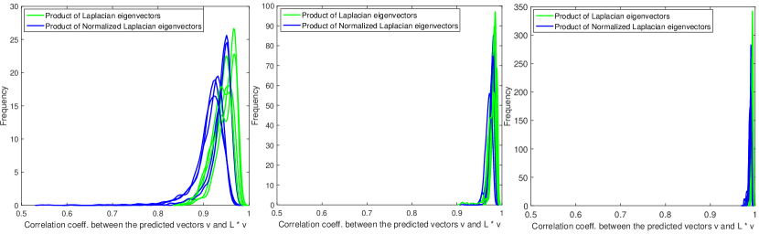
Figure 5: Smoothed probability density functions of vector correlation coefficients between $w_{i}^{S_{1}}\otimes w_{j}^{S_{2}}$ and $L_{S_{1}\otimes S_{2}}(w_{i}^{S_{1}}\otimes w_{j}^{S_{2}})$ are represented using a solid green line, while between $v_{i}^{S_{1}}\otimes v_{j}^{S_{2}}$ and $L_{S_{1}\otimes S_{2}}(v_{i}^{S_{1}}\otimes v_{j}^{S_{2}})$ are represented using a solid blue line. Watts-Strogatz random graphs have 50 and 30 vertices. Probability density functions are drawn for each of the edge density level 10%, 30% and 65%, respectively.

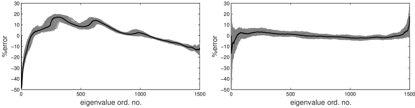
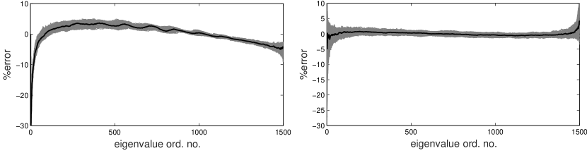
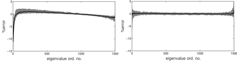
Figure 6: Distribution of percentage errors in estimated Laplacian spectra of the Kronecker product of Watts-Strogatz graphs (50 and 30 vertices) compared to original ones. Left hand side is reserved for the spectrum of the eigenvectors $w_{i}^{S_{1}}\otimes w_{j}^{S_{2}}$ and right hand side for the spectrum of the eigenvectors $v_{i}^{S_{1}}\otimes v_{j}^{S_{2}}$. Rows correspond to the edge density levels of 10%, 30% and 65%.

3.2 Barabási-Albert graphs

In this section we present a behavior of the eigenvectors and eigenvalues of the Kronecker product of two graphs which are Barabási-Albert graphs. For this type of graph, the situation is not significantly different compared to the previous two types concerning correlation coefficients of the estimated eigenvalues. In all cases $w_{i}^{S_{1}}\otimes w_{j}^{S_{2}}$ eigenvectors express better properties, since their correlation coefficients are above 0.9 in most of the cases, while the correlation coefficients of the $v_{i}^{S_{1}}\otimes v_{j}^{S_{2}}$ eigenvectors are in interval (0.7, 0.9) most of cases (see Figure 7), for the edge density levels of 10%, 30%, and 65%.

Also, we notice that the estimated eigenvalues corresponding to the eigenvectors $w_{i}^{S_{1}}\otimes w_{j}^{S_{2}}$ are more stable than the eigenvalues corresponding to the eigenvectors $v_{i}^{S_{1}}\otimes v_{j}^{S_{2}}$. From Figure 8 it can be noticed that the error ranges (which correspond to edge density levels of 10%, 30% and 65%) between the estimated and original spectrum are less for the first approximation (left panels) than for the second one, which are at the same time more distorted (right panels). The characteristic shape of error distribution for the estimated spectrum corresponding to the eigenvectors $w_{i}^{S_{1}}\otimes w_{j}^{S_{2}}$ remains similar as in the previous subsection. This includes a sudden jump at the beginning followed by a gradual decrease across various network density levels we tested. Unlike the previous subsection, the estimated spectrum corresponding to the eigenvectors $v_{i}^{S_{1}}\otimes v_{j}^{S_{2}}$ has a sudden jump at the beginning and the error ranges are a little bit higher for all edge densities (right panels of Figure 8). When the edge density is from 50% to 65%, the characteristic shape for the second approximation (right panels) is a bit different than usual. It could be noticed sudden jump in the middle of graphs, but in the same time error narrowing for the largest eigenvalues.

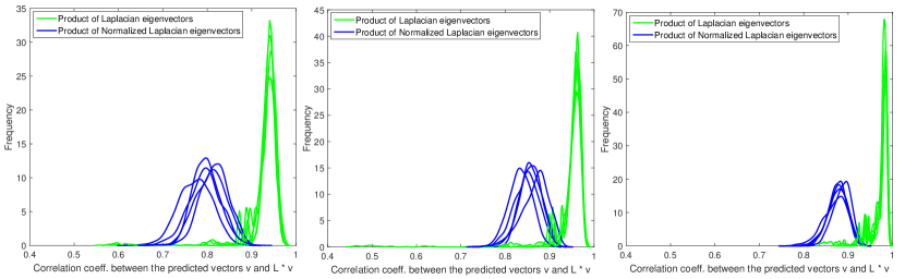
Figure 7: Smoothed probability density functions of vector correlation coefficients between $w_{i}^{S_{1}}\otimes w_{j}^{S_{2}}$ and $L_{S_{1}\otimes S_{2}}(w_{i}^{S_{1}}\otimes w_{j}^{S_{2}})$ are represented using a solid green line, while between $v_{i}^{S_{1}}\otimes v_{j}^{S_{2}}$ and $L_{S_{1}\otimes S_{2}}(v_{i}^{S_{1}}\otimes v_{j}^{S_{2}})$ are represented using a solid blue line. Barabási-Albert random graphs have 50 and 30 vertices. Probability density functions are drawn for each of the edge density 10%, 30% and 65%, respectively.

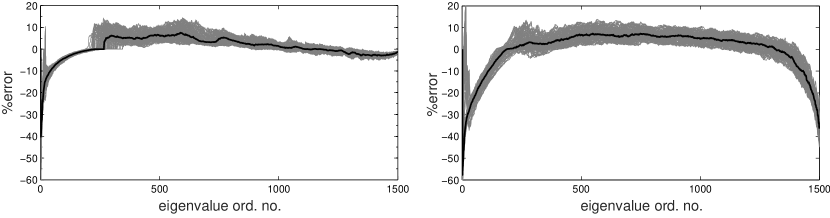
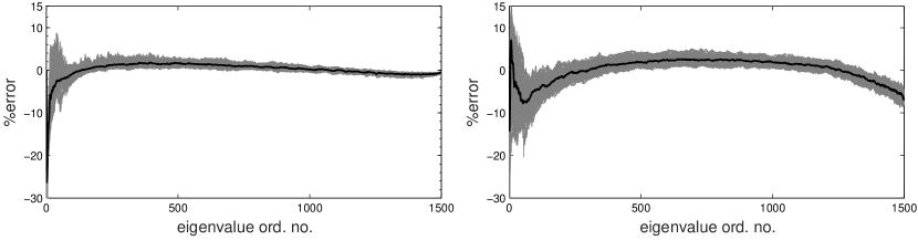
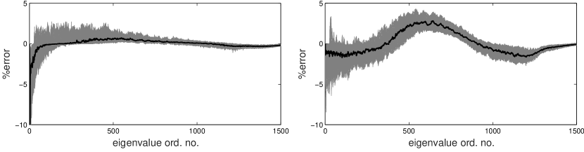
Figure 8: Distribution of percentage errors in estimated Laplacian spectra of the Kronecker product of Barabási-Albert graphs (50 and 30 vertices) compared to original ones. Left hand side is reserved for the spectrum of the eigenvectors $w_{i}^{S_{1}}\otimes w_{j}^{S_{2}}$ and right hand side for the spectrum of the eigenvectors $v_{i}^{S_{1}}\otimes v_{j}^{S_{2}}$. Rows correspond to the edge density levels of 10%, 30%, and 65%.

4 Conclusion

Although the relationships between spectral properties of a product graph and those of its factor graphs have been known for the standard products, characterization of Laplacian spectrum and eigenvectors of the Kronecker product of graphs using the Laplacian spectra of the factors has remained an open problem to date. In this work we proposed a novel approximation method for estimating the Laplacian spectrum and the corresponding eigenvectors of the Kronecker product of graphs knowing the eigenvalues and eigenvectors of factor graphs. The estimated eigenvalues and eigenvectors were compared to the original ones with regard to different types of random networks and theirs edge density levels. Moreover, the properties of the novel approximation were compared with the approximation proposed by Sayama. Although both approximations were designed using a few mathematically incorrect assumptions, the obtained estimations of the spectra are very close to the numerically calculated spectra with percentage errors constrained within a $\pm$10% range for most eigenvalues. Here, we give a theoretical explanation of why the estimated eigenvalues for the random graphs become more accurate to the real values when the network grows or the edge density level increases. This explains the fact that a distribution of percentage errors between estimated and original spectra becomes almost uniformly distributed around 0. In this paper we also presented some novel theoretical results related to the certain correlation coefficients corresponding to the estimated and original vectors. Here, we provide an exact formula of how some of these correlation coefficients can be explicitly calculated, as well as their expected values for some types of random networks.

As it was mentioned earlier, in this and Sayama’s paper, these approximations have many theoretical limitations, because of the mathematically incorrect assumptions and there is no rigorous mathematical explanation of why and how the proposed methods work. That is why a design of spectral estimation algorithms will be an important direction of future research, as well as their theoretical explanations. Moreover, it would be very important to see how the estimated eigenvalues and eigenvectors are suitable for complete spectral decomposition of the graph, where all eigenvalues and eigenvectors are included to replace original ones. According to some preliminary results we have already obtained by incorporating these approximations in the GCRF model, a good behaviour of these approximations presented in this paper have been experimentally confirmed too. Moreover, we obtained that the presented estimations can be a good staring point for other applications and further improvements of Laplacian spectrum of the Kronecker product of graphs.

References

• Pržulj [2011] Nataša Pržulj. Protein-protein interactions: Making sense of networks via graph-theoretic modeling. Bioessays, 33(2):115–123, 2011.
• Shi and Malik [2000] Jianbo Shi and Jitendra Malik. Normalized cuts and image segmentation. Departmental Papers (CIS), page 107, 2000.
• Arsić et al. [2016] Branko Arsić, Milan Bašić, Petar Spalević, Miloš Ilić, and Mladen Veinović. Facebook profiles clustering. In Proceedings of the 6th International Conference on Information Society and Technology (ICIST 2016), pages 154–158, Kopaonik, Serbia, 2016. Society for Information Systems and Computer Networks.
• Bašić [2014] Milan Bašić. Which weighted circulant networks have perfect state transfer? Information Sciences, 257:193–209, 2014.
• Milo et al. [2002] Ron Milo, Shai Shen-Orr, Shalev Itzkovitz, Nadav Kashtan, Dmitri Chklovskii, and Uri Alon. Network motifs: simple building blocks of complex networks. Science, 298(5594):824–827, 2002.
• Girvan and Newman [2002] Michelle Girvan and Mark EJ Newman. Community structure in social and biological networks. Proceedings of the national academy of sciences, 99(12):7821–7826, 2002.
• De Domenico et al. [2013] Manlio De Domenico, Albert Solé-Ribalta, Emanuele Cozzo, Mikko Kivelä, Yamir Moreno, Mason A Porter, Sergio Gómez, and Alex Arenas. Mathematical formulation of multilayer networks. Physical Review X, 3(4):041022, 2013.
• Arenas et al. [2007] Alex Arenas, Jordi Duch, Alberto Fernández, and Sergio Gómez. Size reduction of complex networks preserving modularity. New Journal of Physics, 9(6):176, 2007.
• Skardal and Restrepo [2012] Per Sebastian Skardal and Juan G Restrepo. Hierarchical synchrony of phase oscillators in modular networks. Physical Review E, 85(1):016208, 2012.
• Leskovec et al. [2010] Jure Leskovec, Deepayan Chakrabarti, Jon Kleinberg, Christos Faloutsos, and Zoubin Ghahramani. Kronecker graphs: An approach to modeling networks. Journal of Machine Learning Research, 11(Feb):985–1042, 2010.
• Sole-Ribalta et al. [2013] Albert Sole-Ribalta, Manlio De Domenico, Nikos E Kouvaris, Albert Diaz-Guilera, Sergio Gomez, and Alex Arenas. Spectral properties of the laplacian of multiplex networks. Physical Review E, 88(3):032807, 2013.
• Kivelä et al. [2014] Mikko Kivelä, Alex Arenas, Marc Barthelemy, James P Gleeson, Yamir Moreno, and Mason A Porter. Multilayer networks. Journal of complex networks, 2(3):203–271, 2014.
• Elsässer et al. [2004] Robert Elsässer, Burkhard Monien, Robert Preis, and Andreas Frommer. Optimal diffusion schemes and load balancing on product graphs. Parallel Processing Letters, 14(01):61–73, 2004.
• Cvetković and Gutman [2011] Dragoš M Cvetković and Ivan Gutman. Selected topics on applications of graph spectra. Matematicki institut SANU, 2011.
• Cvetković and Simić [2011] Dragoš Cvetković and Slobodan Simić. Graph spectra in computer science. Linear Algebra and its Applications, 434(6):1545–1562, 2011.
• Sayama [2016] Hiroki Sayama. Estimation of laplacian spectra of direct and strong product graphs. Discrete Applied Mathematics, 205:160–170, 2016.
• Brouwer and Haemers [2011] Andries E Brouwer and Willem H Haemers. Spectra of graphs. Springer Science & Business Media, 2011.
• Cvetković et al. [1980] Dragoš M Cvetković, Michael Doob, and Horst Sachs. Spectra of graphs: theory and application, volume 87. Academic Pr, 1980.
• Merris [1994] Russell Merris. Laplacian matrices of graphs: a survey. Linear algebra and its applications, 197:143–176, 1994.
• Glass and Obradovic [2017] Jesse Glass and Zoran Obradovic. Structured regression on multiscale networks. IEEE Intelligent Systems, 32(2):23–30, 2017.
• Barik et al. [2015] Sasmita Barik, Ravindra B Bapat, and S Pati. On the laplacian spectra of product graphs. Applicable Analysis and Discrete Mathematics, pages 39–58, 2015.
• Godsil and Royle [2001] Chris Godsil and Gordon F. Royle. Algebraic Graph Theory. Graduate Texts in Mathematics. Springer New York, 2001. ISBN 9780387952413.
• Brockwell and Davis [1991] Peter J. Brockwell and Richard A. Davis. Time Series: Theory and Methods. Graduate Texts in Mathematics. Springer, 1991. ISBN 978-1-4419-0319-8.
• Furtula and Gutman [2015] Boris Furtula and Ivan Gutman. A forgotten topological index. J. Math. Chem., 53:1184–1190, 2015.
• Gutman and Das [2004] Ivan Gutman and Kinkar C. Das. The first zagreb index 30 years after. MATCH Commun.Math. Comput. Chem., 50:83–92, 2004.
• Che and Chen [2016] Zhongyuan Che and Zhibo Chen. Lower and upper bounds of the forgotten topological index. MATCH Commun. Math. Comput. Chem, 76(3):635–648, 2016.
• Chung and Radcliffe [2011] Fan Chung and Mary Radcliffe. On the spectra of general random graphs. The electronic journal of combinatorics, 18(1):P215, 2011.
• Leveque [2014] Olivier Leveque. https://mathoverflow.net/questions/176689/limiting-empirical-spectral-distribution-of-the-laplacian-matrix-on-an-erdos-ren. Mathoverflow, 2014.