Progressive Neural Image Compression
with Nested Quantization and Latent Ordering

Abstract

We present PLONQ, a progressive neural image compression scheme which pushes the boundary of variable bitrate compression by allowing quality scalable coding with a single bitstream. In contrast to existing learned variable bitrate solutions which produce separate bitstreams for each quality, it enables easier rate-control and requires less storage. Leveraging the latent scaling based variable bitrate solution, we introduce nested quantization, a method that defines multiple quantization levels with nested quantization grids, and progressively refines all latents from the coarsest to the finest quantization level. To achieve finer progressiveness in between any two quantization levels, latent elements are incrementally refined with an importance ordering defined in the rate-distortion sense. To the best of our knowledge, PLONQ is the first learning-based progressive image coding scheme and it outperforms SPIHT, a well-known wavelet-based progressive image codec.

1 Introduction

Recent developments of learning based lossy image [1, 2, 3, 4, 5, 6] and video compression [7, 8, 9, 10, 11] schemes have witnessed remarkable success in achieving state-of-the-art rate-distortion (R-D) performance compared to traditional codecs in a variety of benchmark datasets. Leveraging the expressiveness of deep auto-encoder networks, these works compress an image by learning a nonlinear transform between the image and the latent, along with a learned entropy model in order to encode the quantized latent. The optimization objective is often framed as a tradeoff between the Rate (R), the amount of bits used to encode the source, and the Distortion (D), the distance between the input source and the reconstructed source:

$$\min_{\theta}\mathbb{E}_{x}\left[D_{\theta}(x)+\beta R_{\theta}(x)\right]$$

where $\beta$ is the tradeoff parameter and $\theta$ represents the model parameters. During training, $\theta$ is typically optimized from end-to-end using stochastic gradient descent.

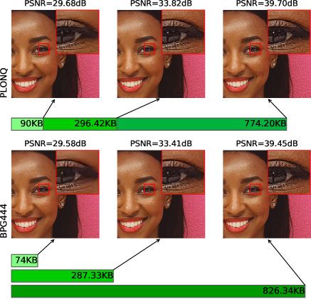
Fig. 1: Qualitative comparison³ of PLONQ and BPG444. For PLONQ (top), reconstructions at different qualities can be obtained by truncating a single bitstream, whereas for BPG444 (bottom), separate bitstreams have to be stored one for each bitrate option.

Most of these learning based methods, however, are not readily suitable for large scale deployment because in most of learning based codecs [1, 2, 4, 5, 6], separate models need to be trained to accommodate different bitrate targets. To address this issue, Choi et al. [13] proposed a conditional auto-encoder to make the parameters in the encoder and decoder network be dependent on the rate distortion trade-off parameter, $\beta$ so that a single model can adapt to different rate-distortion tradeoffs. More recently, [14, 15, 3] proposed latent scaling based variable bitrate compression which is essentially learning to adjust the quantization step size of the latents. After training, the interpolation of the learned scaling parameters can lead to continuous variable bitrate performance. Other attempts [16, 17] have also been made to address the variable bitrate targets.

While variable bitrate solutions make learning based image compression more practical for deployment, they require storing multiple copies of the latent code used for different bitrates, i.e., quality levels [14, 15]. In contrast, with progressive coding, the transmitted bitstream is completely embedded, which be truncated at various points and reconstructed into a series of lower bitrate images [18]. Therefore it significantly reduces storage and simplifies rate control.

Existing literature [19] allowing for progressiveness adopted an encoder parameterized by a recurrent neural network, so that it can incrementally transmit the quantized latents. However, the inference time is slow for recurrent neural networks and their performance is not competitive with BPG or the family of hyperprior based solutions [1, 6]. In this study, we present PLONQ, a Progressive coding based neural image compression method via Latent Ordering and Nested Quantization. PLONQ is built upon the latent scaling based solution while being amenable for deployment. In summary, our work has the following main contributions:

1. We demonstrate the effectiveness of a simple latent scaling based variable bitrate solution using a pretrained high bitrate model without any retraining, dubbed as Naive Scaling.

2. We propose nested quantization which enables progressive coding across different quantization levels.

3. We find sorting latent variables element-wise by prior standard deviation works well to obtain better truncation points between two quantization levels.

Combining nested quantization with latent ordering, PLONQ achieves better performance than SPIHT, a well-known progressive coding algorithm, and performs on par with BPG at high bitrate.

2 Latent Scaling

We base our method on the mean-scale hyperprior model [2] and inherit the notations therein: we denote the input image by $x$, and the analysis transform (encoder) and synthesis transform (decoder) by $g_{a}$ and $g_{s}$ respectively. Both $g_{a}$ and $g_{s}$ are parameterized by convolutional neural networks. The output of the encoder is the continuous latent space tensor $y=g_{a}(x)$, which has a Gaussian prior with its mean $\mu$ and standard derivation $\sigma$ predicted based on hyper latent. We use $P(\cdot)$ to denote the probability value on an interval and use $\mathbb{P}(\cdot)$ to denote the discretized probability value.

The idea of latent scaling [14, 15], is to apply a scaling factor $s$ to the latent $y$. Because the quantization step size is fixed, this leads to a different tradeoff between rate and distortion. For ease of exposition we consider a single latent variable, so that both $y$ and $s$ are scalar. The diagram of the latent scaling is depicted in Fig 2. The latent $y$ is scaled with $1/s$, where we restrict $s>1$. In the quantization step (shown in the blue shaded rectangle in Fig 2, we choose to center the scaled latent $y/s$ by its prior mean $\mu/s$, apply the rounding operator $\lfloor\cdot\rceil$ on $(y-\mu)/s$ (so that the estimated mean $\mu$ learned by the hyper-encoder is on the grid), and then add the offset $\mu/s$ back. The dequantized latent $y(s)$ is obtained by multiplying $s$ after the quantization block, i.e.

$$\centering y(s)\triangleq\@add@centering \left\lfloor\frac{y-\mu}{s}\right\rceil s+\mu.$$

The prior probability of $y(s)$ used in entropy coding can be derived from the original prior density by change of variables:

$$\mathbb{P}_{Y(s)}(y(s))=\mathbb{P}_{\frac{Y(s)}{s}}\left(\frac{y(s)}{s}\right)=\mathbb{P}_{\frac{Y(s)}{s}}\left(\left\lfloor\frac{y-\mu}{s}\right\rceil+\frac{\mu}{s}\right)$$

$$=\int^{\lfloor(y-\mu)/s\rceil+\frac{1}{2}}_{\lfloor(y-\mu)/s\rceil-\frac{1}{2}}p_{(y-\mu)/s}(u)du=\int^{y^{+}(s)}_{y^{-}(s)}p_{y}(v)dv,$$ (1)

where $y^{+}(s)\triangleq y(s)+\frac{s}{2}$ and $y^{-}(s)\triangleq y(s)-\frac{s}{2}$ can be interpreted as the upper and lower boundary of the effective quantization bin.

Note in Eq. (1), we first apply the change of variable formula for discrete random variables in the first line, and then apply a change of variable formula for continuous random variables from the second to the third line. According to Eq (1), applying the scaling $s$ is equivalent to changing the quantization bin width from 1 to $s$. Hence increasing the latent scaling value $s$ will lead to larger quantization bin width and hence smaller bitrate in the entropy coding, as well as larger distortion of the reconstructed image.

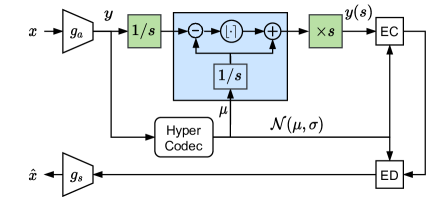
Fig. 2: Mean-scale hyperprior with latent scaling. EC is entropy encoder, ED is entropy decoder. Note that scaling $s$ is applied to latent $y$ after being passed to hyper codec so that the prior parameters $\mu,\sigma$ can be shared by $y(s)$ for different $s$.

3 Nested Quantization

In this section, we introduce nested quantization, one of the key techniques we use to construct a progressive bitstream. Let us start with a pre-trained mean-scale hyperprior model and consider $K$ quantization levels defined by a set of $K$ latent scaling factors $\{s_{1},s_{2},...,s_{K}\}$ with $s_{1}<s_{2}<...<s_{K}$. We define a scheme, where for each level, the same scaling factor is applied across all latent elements. Effectively, these $K$ quantization bin sizes translate into $K$ different bitrate options. We name this simple single-model variable-bitrate scheme as Naive Scaling. Despite its simplicity, In Section 5 we show that it achieves performance comparable to a more involved scheme [14] that uses $K$ sets of learnable per-channel scaling factors optimized for $K$ Lagrange multipliers $\beta$.

Naturally, the information contained in the discrete latents quantized with different scaling factors follows a total ordering – the one quantized with smaller bins is always a refinement of the larger. Progressiveness across different quantization levels can then be achieved if we can find a way to embed the information of coarse level quantization into its finer counterpart. Indeed, a principled way to achieve this progressiveness is to encode a finer quantized latent with probabilities conditioned on its coarser quantized values. We term this scheme nested quantization and detail it next.

In nested quantization, the encoding happens in $K$ stages. In the first stage, we quantize $y$ with the coarsest bin $s_{K}$ and encode it with $\mathbb{P}\left(y(s_{K})\right)$ as defined in Eq (1). In the remaining stages, we iteratively refine the quantization of $y$ using bin width $s_{k-1}$ that is one level finer than $s_{k}$, for $1\leq k<K$. In particular, we encode an extra piece of information of $y$ quantized to a finer grained level through the conditional probability below,

$$\mathbb{P}\left(y(s_{k})|y(s_{i})_{i>k}\right)= P(I_{k})/P(I_{k+1})\text{ for }1\leq k<K,$$

where $P(I)\triangleq\int_{v\in I}p_{y}(v)dv$, and $I_{k}$ is defined below as iterative intersections of quantization bins:

$$I_{K} \triangleq\left[y^{-}(s_{K}),y^{+}(s_{K})\right],\text{ and }$$

$$I_{k} \triangleq I_{k+1}\cap\left[y^{-}(s_{k}),y^{+}(s_{k})\right]\text{ for }1\leq k<K.$$

An illustration of this procedure with $K=2$ can be found in Fig 3. The code generated by these $K$ stages form a bitstream that embeds $K$ different bitrates, and the total length of the bitstream is

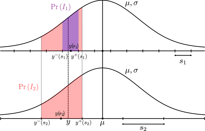
Fig. 3: Illustration of nested quantization of $y$ when $K=2$.

$$\underbrace{\log\frac{1}{\mathbb{P}\left(y\left(s_{K}\right)\right)}}_{\begin{subarray}{c}\text{codeword length w.r.t.}\\ \text{coarsest quant. level $s_{K}$}\end{subarray}}+\sum_{1\leq k<K}\underbrace{\log\frac{1}{\mathbb{P}\left(y\left(s_{k}\right)|y\left(s_{i}\right)_{i>k}\right)}}_{\begin{subarray}{c}\text{codeword length w.r.t. refined}\\ \text{information from }s_{k+1}\text{ to }s_{k}\end{subarray}}=\log\frac{1}{P(I_{1})}.$$

There are two issues of this scheme as can be seen from the above equation: (1) conditional probability computation requires tracking of intersected quantization boundaries, which adds to implementation complexity; (2) the sum of codeword length $\log 1/P(I_{1})$ is in general larger than the codeword length with respect to the finest quantization level $\log 1/\mathbb{P}\left(y(s_{1})\right)$.

These two issues can be resolved if we consider a set of fully nested quantization levels where the set of grid points of the coarser quantization bin is always a subset of the finer. In other words, we can define quantization levels in such a way that $I_{k}=I_{k+1}\cap\left[y^{-}(s_{k}),y^{+}(s_{k})\right]=\left[y^{-}(s_{k}),y^{+}(s_{k})\right]$, which simplifies the above equation as

$$\log\frac{1}{\mathbb{P}\left(y\left(s_{K}\right)\right)}+\sum_{1\leq k<K}\log\frac{\mathbb{P}\left(y\left(s_{k+1}\right)\right)}{\mathbb{P}\left(y\left(s_{k}\right)\right)}=\log\frac{1}{\mathbb{P}\left(y\left(s_{1}\right)\right)}.$$

With this we are able to preserve the performance of the highest bit-rate model at the end of the progressive coding procedure.

In practice, we find it beneficial to further generalize this idea to quantization levels with uneven grid, which is applied to PLONQ and explained in Section 5.

4 Latent Ordering

To obtain more truncation points in the embedded bitstream between two quantization levels, latent variables can be refined incrementally instead of all at once. The problem is how to find the optimal order to refine them, so that wherever the resulting bitstream is truncated, the reconstruction has the highest possible quality. The embedding principle states the latent that reduces the distortion the most per bit should be coded first [20].

Depending on the embedding granularity, the latent tensor $y$ is divided into coding units $\{y_{1},...,y_{N}\}$. All the latent elements in one coding unit are refined together at once, corresponding to one truncation point. For the latent tensor with shape $(C,H,W)$, we have considered three types of coding unit for the latent: (1) one channel, (2) one pixel, and (3) one element, which corresponds to a latent slice of size $(1,H,W)$, $(C,1,1)$ and $(1,1,1)$ respectively.

Given an order $\rho=(\rho_{1},...,\rho_{N})$, ordered coding units $y_{\rho}=(y_{\rho_{1}},...,y_{\rho_{N}})$ are refined one by one from scaling $s_{k}$ to $s_{k-1}$. In mean-scale hyperprior model, the priors of latent elements are independent conditioned on the hyper latent. Thus the bitrate increase of refining $y_{\rho_{t}}$, i.e. $\Delta R(y_{\rho_{t}})=-\log\mathbb{P}\left(y_{\rho_{t}}(s_{k-1})|y_{\rho_{t}}(s_{k})\right)$ can be calculated in parallel once the hyper latent is decoded and it is independent of $\rho$. However, with a nonlinear ConvNet decoder, the reduction in distortion depends on the all other ordered coding units, i.e. $\Delta D\left(y_{\rho_{t}}|y_{\rho}\right)=D\left(y_{\rho}(t-1)\right)-D\left(y_{\rho}(t)\right)$, where $y_{\rho}(t)=(y_{\rho_{\leq t}}(s_{k-1}),y_{\rho_{>t}}(s_{k}))$, and $D(y)=\text{MSE}(x,g_{s}(y))$ is the distortion for latent $y$. Thus refining ordered latent by $\rho$ leads to a set of R-D points $\mathcal{H}(\rho)=\{\sum_{i\leq t}\Delta R(y_{\rho_{i}}),\sum_{i\leq t}\Delta D(y_{\rho_{i}}|y_{\rho})\}_{t=1}^{N}$. The optimal order $\rho^{*}$ is the one under which the convex hull of $\mathcal{H}(\rho^{*})$ is better than that of other orders in the Pareto optimal sense [21].

Following embedding principle, $\frac{\Delta D}{\Delta R}$ should be sorted in descending order. We use a greedy procedure to calculate $\frac{\Delta D}{\Delta R}$ under an initial order, e.g. the index order, as the first sorting criterion. The second criterion is the bitrate $\Delta R$ of a coding unit, because we observe sorting latent channels by $\Delta R$ and by $\frac{\Delta D}{\Delta R}$ lead to similar R-D curve. Since the standard derivation $\sigma$ of the latent prior is correlated to the expected bitrate, it is considered as the third criterion. Note that the first two criteria incur bitrate overhead for coding the order, while the last one does not since $\sigma$ is already known when decoding $y$.

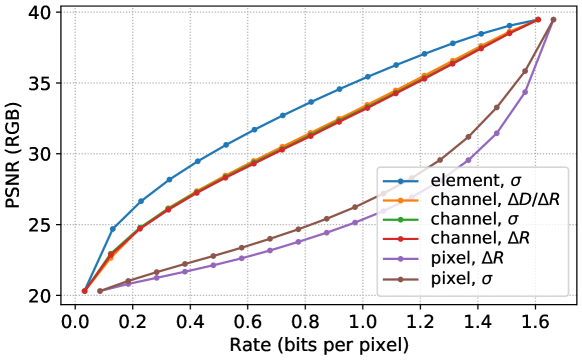
Fig. 4: Coding units are incrementally refined between two quantization levels ($s_{2}=10,000$, i.e. $y(s_{2})=\mu$, $s_{1}=1$) according to a latent order determined by a sorting criterion.

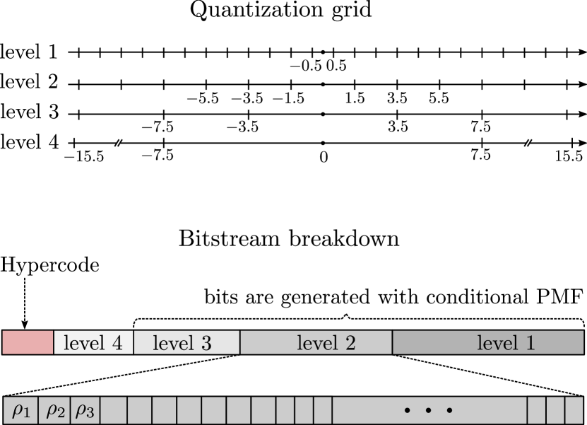
(a) Quantization levels and breakdown of components in the bitstream.

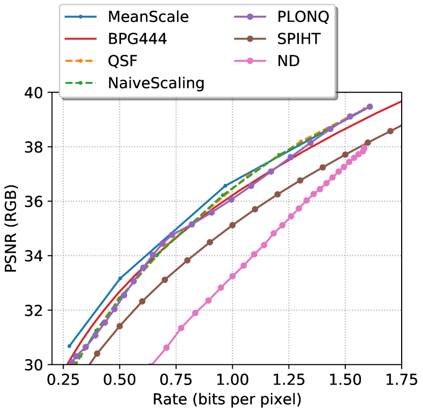
(b) Rate-distortion comparison on
JPEG AI testset[12]

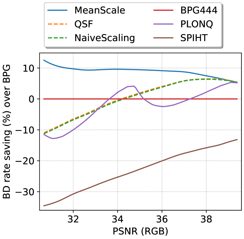
(c) BD-rate savings relative to BPG444 on
JPEG AI testset[12]

Fig. 5: Illustration of PLONQ, and performance comparison of PLONQ and baseline schemes described in Table 1.

We experimented with 6 combinations of coding unit and sorting criterion, and find the one with the best R-D performance. The latent ordering results on the JPEG AI testset [12] is shown in Fig 4. It is natural to choose channels as the coding unit because each channel is usually considered as a learned feature map in ConvNet codec. Indeed channel ordering has been studied in ordered representation learning with nested dropout of latent channels [22] and progressive decoding with a channel-wise auto-regressive prior model (Section $G$ in the appendix of [1]). With channel-wise ordering, the more principled sorting criterion $\frac{\Delta D}{\Delta R}$ performs slightly better than the alternatives while being much more expensive to calculate. When using a single element as coding unit, $\frac{\Delta D}{\Delta R}$ becomes too expensive to calculate, but sorting latent elements by $\sigma$ performs much better than sorting channels by any criterion, and does not require to transmit the latent ordering, thus sorting element units by $\sigma$ is chosen for latent ordering in PLONQ.

5 Experiment

In this section, we show experimental results of Naive Scaling, a plug-and-play variable bitrate solution and PLONQ, our proposed progressive coding scheme, compared against a set of baseline solutions listed in Table 1.

For PLONQ, we use four quantization levels as the basis for nested quantization, and a mean-scale hyperprior ([2] without spatial autoregresssive context) trained with $\beta=1e-4$ as the base model. We enforce the quantization grid to be fully nested in the sense that a coarser quantization grid is always aligned with a finer one. In practice, we find it beneficial to adopt an uneven quantization grid design, where the center bin size can be different from the other bin sizes. Through experiments we identify the set of quantization levels illustrated in Fig 5(a) as a good design choice.

To favor fine-grained rate-control, PLONQ computes an image-specific ordering $\rho$ of latent elements and then incrementally updates the latent with finer quantization level element by element following the order. Based on the analysis in Section 4, we adopt the order computed by sorting the per-element standard deviation $\sigma$ from the output of the hyper decoder. An illustration of breakdown of the bitstream can be found in lower half of Fig 5(a). Note that the use of image-specific latent element ordering incurs no extra bit overhead, since the ordering can be derived after hypercode is obtained.

Table 1: Baseline image compression schemes

Label	Description
MeanScale	Mean-Scale hyperprior model ([2] without spatial autoregresssive context). Four models trained separately with $\beta$=1e-4, 3e-4, 1e-3, and 3e-3 for 2 million steps.
BPG444	Better Portable Graphics[24] (HEVC All-intra)
QSF	Quality Scaling Factor[14]. 8 sets of learnable per-channel latent scaling factors trained from $\beta=$1e-4 to 5e-2 on a pre-trained and freezed MeanScale($\beta$=1e-4) model.
NaiveScaling	Constant latent scaling factors $s=1,2,\ldots,8$ applied to a pre-trained MeanScale($\beta$=1e-4) model.
ND	MeanScale($\beta$=1e-4) with Nested Dropout[22] training.
SPIHT	Set Partitioning In Hierarchical Trees[18]

5.1 Performance evaluation

We evaluate the performance of PLONQ against an array of baseline schemes outlined in Table 1, which divides into three categories (as delimited in the table): (1) multi-model compression scheme (2) non-progressive single model variable bitrate scheme (3) progressive compression scheme. Among them, BPG444 and SPIHT are traditional codecs and the rest are learning-based codecs.

Fig 5(b) and 5(c) show the RD curve (bpp vs PSNR) as well as the BD-rate[25] saving relative to BPG444 computed on JPEG AI dataset [12]. The markers on the progressive solution RD curves indicate the achievable rate options. As shown in the two figures, PLONQ is significantly better than the learned nested dropout [22]. Further PLONQ outperforms the well-known conventional progressive coding scheme SPIHT [18] by a considerable margin uniformly across the whole bpp range, and it is even competitive to the non-progressive coding scheme BPG444 at high bpp regime. The same observation is made on Kodak and Tecnick dataset, for which the results can be found in the appendix.

6 Conclusion

We have introduced PLONQ, a learning based progressive image codec using nested quantization and latent ordering. It uniformly outperforms the existing wavelet-based progressive image codec SPIHT and matches or even outperforms BPG444 in the high bitrate region. The effectiveness of PLONQ proves itself to be a solid baseline for learning based progressive codec and gives the first glimpse of its potential to enable progressive neural video coding.

Appendix A Dataset preprocessing

The following two image in the original JPEG AI test dataset incur more GPU memory than is available to us for mean-scale hyper-prior inference, and thus we cropped it to 3680x2160 (cropped from top) for all our experiments.

00014_TE_3680x2456.png

00015_TE_3680x2456.png

Appendix B Evaluation of BPG444 and SPIHT

BPG444 [24] results are generated with the following command:

bpgenc -e x265 -q [qp] -f 444

-o [output file] [input file]

The results on Kodak dataset (shown in 6) is validated against that provided in
https://github.com/tensorflow/compression/
blob/master/results/image_compression/
kodak/PSNR_sRGB_RGB/bpg444.txt

SPIHT[18] results are obtained by encoding each image with a target bpp of 2.0 and decoding by truncating the bitstream by a step size of 0.1bpp. The curves are generated by averaging PSNR across images for each of the fixed bpps.

Appendix C Additional experiment results on Kodak and Tecnick testset

Fig 6 and 7 show the performance comparison of PLONQ and baseline schemes described in Table 1 on Kodak; Fig 8 and 9 shows the results on Tecnick test dataset (100 images with 1200 x 1200 resolution).

Fig. 6: Rate-distortion comparison on Kodak.

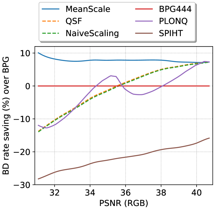
Fig. 7: BD-rate savings relative to BPG444 on Kodak.

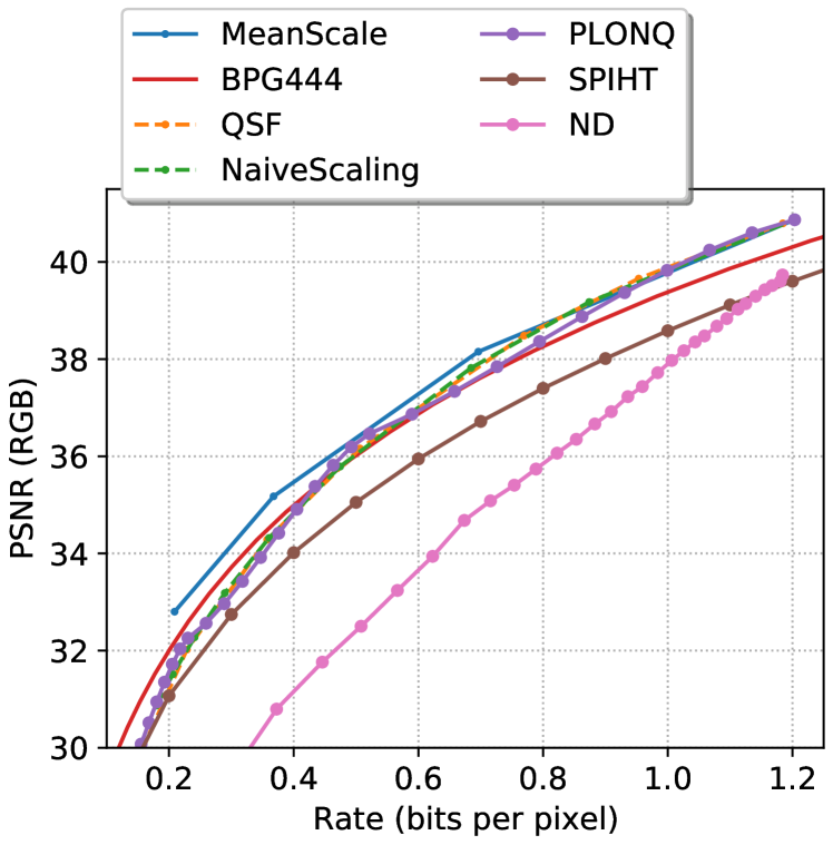
Fig. 8: Rate-distortion comparison on Tecnick testset.

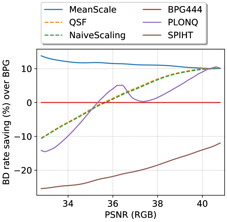
Fig. 9: BD-rate savings relative to BPG444 on Tecnick testset.

References

- [1] David Minnen and Saurabh Singh, “Channel-wise Autoregressive Entropy Models for Learned Image Compression,” in IEEE International Conference on Image Processing (ICIP), 2020.
- [2] Johannes Ballé David Minnen and George D. Toderici, “Joint Autoregressive and Hierarchical Priors for Learned Image Compression ,” in Advances in Neural Information Processing Systems 31 (NeurIPS), 2018.
- [3] Tong Chen, Haojie Liu, Zhan Ma, Qiu Shen, Xun Cao, and Yao Wang, “Neural Image Compression via Non-Local Attention Optimization and Improved Context Modeling,” 2019.
- [4] Zhengxue Cheng, Heming Sun, Masaru Takeuchi, and Jiro Katto, “Learned Image Compression With Discretized Gaussian Mixture Likelihoods and Attention Modules,” in Proceedings of the IEEE/CVF Conference on Computer Vision and Pattern Recognition (CVPR), June 2020.
- [5] Johannes Ballé, Valero Laparra, and Eero P. Simoncelli, “End-to-End Optimized Image Compression,” in International Conference on Learning Representations (ICLR), 2017.
- [6] Johannes Ballé, David Minnen, Saurabh Singh, Sung Jin Hwang, and Nick Johnston, “Variational Image Compression with a Scale Hyperprior,” in International Conference on Learning Representations (ICLR), 2018.
- [7] Eirikur Agustsson, David Minnen, Nick Johnston, Johannes Balle, Sung Jin Hwang, and George Toderici, “Scale-space flow for end-to-end optimized video compression,” in Proceedings of the IEEE/CVF Conference on Computer Vision and Pattern Recognition (CVPR), June 2020.
- [8] Ruihan Yang, Yibo Yang, Joseph Marino, and Stephan Mandt, “Hierarchical Autoregressive Modeling for Neural Video Compression,” in International Conference on Learning Representations (ICLR), 2021.
- [9] Guo Lu, Wanli Ouyang, Dong Xu, Xiaoyun Zhang, Chunlei Cai, and Zhiyong Gao, “DVC: An End-To-End Deep Video Compression Framework,” in Proceedings of the IEEE/CVF Conference on Computer Vision and Pattern Recognition (CVPR), June 2019.
- [10] Amirhossein Habibian, Ties van Rozendaal, Jakub M. Tomczak, and Taco S. Cohen, “Video compression with rate-distortion autoencoders,” in Proceedings of the IEEE/CVF International Conference on Computer Vision (ICCV), October 2019.
- [11] Adam Golinski, Reza Pourreza, Yang Yang, Guillaume Sautiere, and Taco S. Cohen, “Feedback recurrent autoencoder for video compression,” in Proceedings of the Asian Conference on Computer Vision (ACCV), November 2020.
- [12] JPEG AI Testset, 2020, https://jpegai.github.io/test_images/.
- [13] Yoojin Choi, Mostafa El-Khamy, and Jungwon Lee, “Variable Rate Deep Image Compression With a Conditional Autoencoder,” in Proceedings of the IEEE/CVF International Conference on Computer Vision (ICCV), October 2019.
- [14] T. Chen and Z. Ma, “Variable Bitrate Image Compression with Quality Scaling Factors,” in ICASSP 2020 - 2020 IEEE International Conference on Acoustics, Speech and Signal Processing (ICASSP), 2020.
- [15] Ze Cui, Jing Wang, Bo Bai, Tiansheng Guo, and Yihui Feng, “G-VAE: A Continuously Variable Rate Deep Image Compression Framework,” 2020.
- [16] Tiansheng Guo, Jing Wang, Ze Cui, Yihui Feng, Yunying Ge, and Bo Bai, “Variable Rate Image Compression With Content Adaptive Optimization,” in Proceedings of the IEEE/CVF Conference on Computer Vision and Pattern Recognition (CVPR) Workshops, June 2020.
- [17] Jing Zhou, Akira Nakagawa, Keizo Kato, Sihan Wen, Kimihiko Kazui, and Zhiming Tan, “Variable Rate Image Compression Method With Dead-Zone Quantizer,” in Proceedings of the IEEE/CVF Conference on Computer Vision and Pattern Recognition (CVPR) Workshops, June 2020.
- [18] A. Said and W. A. Pearlman, “A New, Fast, and Efficient Image Codec Based on Set Partitioning in Hierarchical Trees,” IEEE Transactions on Circuits and Systems for Video Technology, vol. 6, no. 3, pp. 243–250, 1996.
- [19] George Toderici, Sean M. O’Malley, Sung Jin Hwang, Damien Vincent, David Minnen, Shumeet Baluja, Michele Covell, and Rahul Sukthankar, “Variable Rate Image Compression with Recurrent Neural Networks,” in International Conference on Learning Representations (ICML), 2016.
- [20] David Taubman, Erik Ordentlich, Marcelo Weinberger, and Gadiel Seroussi, “Embedded block coding in JPEG 2000,” Signal Processing: Image Communication, vol. 17, no. 1, pp. 49–72, 2002.
- [21] David Taubman, “High Performance Scalable Image Compression with EBCOT,” IEEE Transactions on image processing, vol. 9, no. 7, pp. 1158–1170, 2000.
- [22] Oren Rippel, Michael Gelbart, and Ryan Adams, “Learning Ordered Representations with Nested Dropout,” in International Conference on Machine Learning, 2014, pp. 1746–1754.
- [23] G. J. Sullivan, “Efficient scalar quantization of exponential and Laplacian random variables,” IEEE Transactions on Information Theory, vol. 42, no. 5, pp. 1365–1374, 1996.
- [24] Fabrice Bellard, Better Portable Graphics, 2014, https://bellard.org/bpg/.
- [25] Gisle Bjontegaard, “Calculation of Average PSNR Differences Between RD-curves,” VCEG-M33, 2001.