Hierarchical Multivariate Directed Acyclic Graph Auto-Regressive (MDAGAR) models for spatial diseases mapping

Abstract

Disease mapping is an important statistical tool used by epidemiologists to assess geographic variation in disease rates and identify lurking environmental risk factors from spatial patterns. Such maps rely upon spatial models for regionally aggregated data, where neighboring regions tend to exhibit similar outcomes than those farther apart. We contribute to the literature on multivariate disease mapping, which deals with measurements on multiple (two or more) diseases in each region. We aim to disentangle associations among the multiple diseases from spatial autocorrelation in each disease. We develop Multivariate Directed Acyclic Graphical Autoregression (MDAGAR) models to accommodate spatial and inter-disease dependence. The hierarchical construction imparts flexibility and richness, interpretability of spatial autocorrelation and inter-disease relationships, and computational ease, but depends upon the order in which the cancers are modeled. To obviate this, we demonstrate how Bayesian model selection and averaging across orders are easily achieved using bridge sampling. We compare our method with a competitor using simulation studies and present an application to multiple cancer mapping using data from the Surveillance, Epidemiology, and End Results (SEER) Program.

Keywords: Areal data analysis; Bayesian hierarchical models; Directed acyclic graphical autoregression; Multiple disease mapping; Multivariate areal data models.

1 Introduction

Spatially-referenced data comprising regional aggregates of health outcomes over delineated administrative units such as counties or zip codes are widely used by epidemiologists to map mortality or morbidity rates and better understand their geographic variation. Disease mapping, as this exercise is customarily called, employs statistical models to present smoothed maps of rates or counts of a disease. Such maps can assist investigators in identifying lurking risk factors (Koch, 2005) and in detecting “hot-spots” or spatial clusters emerging from common environmental and socio-demographic effects shared by neighboring regions. By interpolating estimates of health outcome from areal data onto a continous surface, disease mapping also generates smoothed maps for the small-area scale, adjusting for the sparsity of data or low population size (Berke, 2004; Richardson et al., 2004).

For a single disease, there has been a long tradition of employing Markov random fields (MRFs) (Rua and Held, 2005) to introduce conditional dependence for the outcome in a region given its neighbors. Two conspicuous examples are the Conditional Autoregression (CAR) (Besag, 1974; Besag et al., 1991) and Simultaneous Autoregression (SAR) models (Kissling and Carl, 2008) that build dependence using undirected graphs to model geographic maps. More recently, Datta et al. (2018) proposed a class of Directed Acyclic Graphical Autoregressive (DAGAR) models as a preferred alternative to CAR or SAR models in allowing better identifiability and interpretation of spatial autocorrelation parameters.

Multivariate disease mapping is concerned with the analysis of multiple diseases that are associated among themselves and across space. It is not uncommon to find substantial associations among different diseases sharing genetic and environmental risk factors. Quantification of genetic correlations among multiple cancers have revealed associations among several cancers including lung, breast, colorectal, ovarian and pancreatic cancers (Lindström et al., 2017). Disease mapping exercises with lung and esophageal cancers have also evinced associations among them (Jin et al., 2005). When the diseases are inherently related so that the prevalence of one in a region encourages (or inhibits) occurrence of the other on the same unit, there can be substantial inferential benefits in jointly modeling the diseases rather than fitting independent univariate models for each disease (see, e.g., Knorr-Held and Best, 2001; Kim et al., 2001; Gelfand and Vounatsou, 2003; Carlin et al., 2003; Held et al., 2005; Jin et al., 2005, 2007; Zhang et al., 2009; Diva et al., 2008; Martinez-Beneito, 2013; Marí-Dell’Olmo et al., 2014).

Broadly speaking, there are two approaches to multivariate areal modeling. One approach builds upon a linear transformations of latent effects (see, e.g., Gelfand and Vounatsou, 2003; Carlin et al., 2003; Jin et al., 2005; Zhu et al., 2005; Martinez-Beneito, 2013; Bradley et al., 2015). A different class emerges from hierarchical constructions (Jin et al., 2005; Daniels et al., 2006) where each disease enters the model in a given sequence. Here, we build a class of multivariate DAGAR (MDAGAR) models for multiple disease mapping by building the joint distribution hierarchically using univariate DAGAR models. We build upon the idea in Jin et al. (2005) of constructing GMCAR models, but with some important modifications. As noted in Jin et al. (2005), the order in which the new diseases enter the hierarchical model specifies the joint distribution. Therefore, every ordering produces a different GMCAR model, which leads to an explosion in the number of models even for a modest number of cancers (say, more than 2 or 3 diseases). Alternatively, joint models that are invariant to ordering are constructed using linear transformations of latent random variables (Jin et al., 2007). However, these models are cumbersome and computationally onerous to fit and interpreting spatial autocorrelation becomes challenging.

Our current methodological innovation lies in devising a hierarchical MDAGAR model in conjunction with a bridge sampling algorithm (Meng and Wong, 1996; Gronau et al., 2017) for choosing among differently ordered hierarchical models. The idea is to begin with a fixed ordered set of cancers, posited to be associated with each other and across space, and build a hierarchical model. The DAGAR specification produces a comprehensible association structure, while bridge sampling allows us to rank differently ordered models using their marginal posterior probabilities. Since each model corresponds to an assumed conditional dependence, the marginal posterior probabilities will indicate the tenability of such assumptions given the data. Epidemiologists, then, will be able to use this information to establish relationships among the diseases and spatial autocorrelation for each disease.

The balance of this paper proceeds as follows. Section 2 develops the hierarchical MDAGAR model and introduces a bridge sampling method to select the MDAGAR with the best hierarchical order. Section 3 presents a simulation study to compare the MDAGAR with the GMCAR model and also illustrates the bridge sampling algorithm’s efficacy in selecting the “true” model. Section 4 applies our MDAGAR to age-adjusted incidence rates of four cancers from the SEER database and discusses different cases with respect to predictors. Finally, in Section 5, we summarize some concluding remarks and suggest promotion in the future research.

2 Methods

2.1 Overview of Univariate DAGAR Modeling

Let ${\cal G}=\{{\cal V},{\cal E}\}$ be a graph corresponding to a geographic map, where ${\cal V}=\{1,2,\ldots,k\}$ is a fixed ordering of the vertices of the graph representing clearly delineated regions on the map, and ${\cal E}=\{(i,j):i\sim j\}$ is the collection of edges between the vertices representing neighboring pairs of regions. We denote two neighboring regions by $\sim$. The DAGAR model, proposed by Datta et al. (2018), builds a spatial autocorrelation model for a single outcome on ${\cal G}$ using an ordered set of vertices in ${\cal V}$. Let $N(1)$ be the empty set and let $N(j)=\{j^{\prime}<j:j^{\prime}\sim j\}$, where $j\in{\cal V}\setminus\{1\}$. Thus, $N(j)$ includes geographic neighbors of region $j^{\prime}$ that precede $j$ in the ordered set ${\cal V}$. Let $\{w_{i}:i\in{\cal V}\}$ be a collection of $k$ random variables defined over the map. DAGAR specifies the following autoregression,

$$w_{1} =\epsilon_{1};\quad w_{j}=\sum_{j^{\prime}\in N(j)}b_{jj^{\prime}}w_{j^{\prime}}+\epsilon_{j},\;j=2,\dots,k\;,$$ (1)

where $\epsilon_{j}\mathrel{\overset{\makebox[0.0pt]{\mbox{ind}}}{\sim}}N(0,\lambda_{j})$ with the precision $\lambda_{j}$, and $b_{jj^{\prime}}=0$ if $j^{\prime}\not\in N(j)$. This implies that $\bm{w}\sim N(\bm{0},\tau\bm{Q}(\rho))$, where $\bm{Q}(\rho)$ is a spatial precision matrix that depends only upon a spatial autocorrelation parameter $\rho$ and $\tau$ is a positive scale parameter. The precision matrix $\bm{Q}(\rho)=(\bm{I}-\bm{B})^{\top}\bm{F}(\bm{I}-\bm{B})$, $\bm{B}$ is a $k\times k$ strictly lower-triangular matrix and $\bm{F}$ is a $k\times k$ diagonal matrix. The elements of $\bm{B}$ and $\bm{F}$ are denoted by $b_{jj^{\prime}}$ and $\lambda_{j}$, respectively, where

$$b_{jj^{\prime}}=\left\{\begin{array}[]{l}0\;\mbox{ if }\;j^{\prime}\notin N(j)\;;\\ \frac{\rho}{1+(n_{<j}-1)\rho^{2}}\;\mbox{ if }\;j=2,3,\ldots,k\;,\;j^{\prime}\in N(j)\end{array}\right.\quad\mbox{and}\quad\lambda_{j}=\frac{1+(n_{<j}-1)\rho^{2}}{1-\rho^{2}}\;j=1,2\ldots,k\;,$$ (4)

$n_{<j}$ is the number of members in $N(j)$ and $n_{<1}=0$. The above definition of $b_{jj^{\prime}}$ is consistent with the lower-triangular structure of $\bm{B}$ because $j^{\prime}\notin N(j)$ for any $j^{\prime}\geq j$. The derivation of $\bm{B}$ and $\bm{F}$ as functions of a spatial correlation parameter $\rho$ is based upon forming local autoregressive models on embedded spanning trees of subgraphs of ${\cal G}$ (Datta et al., 2018).

2.2 Motivating multivariate disease mapping

There is a substantial literature on joint modeling of multiple spatially oriented outcomes, some of which have been cited in the Introduction. While it is possible to model each disease separately using a univariate DAGAR, hence independent of each other, the resulting inference will ignore the association among the diseases. This will be manifested in model assessment because the less dependence among diseases that a model accommodates, the farther away it will be from the joint model in the sense of Kullback-Leibler divergence.

More formally, suppose we have two mutually exclusive sets $A$ and $B$ that contain labels for diseases. Let $\bm{y}_{A}$ and $\bm{y}_{B}$ be the vectors of spatial outcomes over all regions corresponding to the diseases in set $A$ and set $B$, respectively. A full joint model $p(\bm{y})$, where $\bm{y}=\left(\bm{y}_{A}^{\top},\bm{y}_{B}^{\top}\right)^{\top}$, can be written as $p(\bm{y})=p(\bm{y}_{A})\times p(\bm{y}_{B}\,|\,\bm{y}_{A})$. Let $C_{1}$ and $C_{2}$ be two nested subsets of diseases in $A$ such that $C_{2}\subset C_{1}\subset A$. Consider two competing models, $p_{1}(\bm{y})=p(\bm{y}_{A})\times p(\bm{y}_{B}\,|\,\bm{y}_{C_{1}})$ and $p_{2}(\bm{y})=p(\bm{y}_{A})\times p(\bm{y}_{B}\,|\,\bm{y}_{C_{2}})$, where $p_{1}(\cdot)$ and $p_{2}(\cdot)$ are probability densities constructed from the joint probability measure $p(\cdot)$ by imposing conditional independence such that $p(\bm{y}_{B}\,|\,\bm{y}_{A})=p(\bm{y}_{B}\,|\,\bm{y}_{C_{1}})$ and $p(\bm{y}_{B}\,|\,\bm{y}_{A})=p(\bm{y}_{B}\,|\,\bm{y}_{C_{2}})$, respectively. Both $p_{1}(\cdot)$ and $p_{2}(\cdot)$ suppress dependence by shrinking the conditional set $A$, but $p_{2}(\cdot)$ suppresses more than $p_{1}(\cdot)$. We show below that $p_{2}(\cdot)$ is farther away from $p(\cdot)$ than $p_{1}(\cdot)$.

A straighforward application of Jensen’s inequality yields $\displaystyle\mathbb{E}_{B|C_{1}}\left[\log\frac{p(\bm{y}_{B}\,|\,\bm{y}_{C_{1}})}{p(\bm{y}_{B}\,|\,\bm{y}_{C_{2}})}\right]\geq 0$, where $\mathbb{E}_{B\,|\,C_{1}}[\cdot]$ denotes the conditional expectation with respect to $p(\bm{y}_{B}\,|\,\bm{y}_{C_{1}})$. Therefore,

$$\begin{split}\mbox{KL}(p\|p_{2})&-\mbox{KL}(p\|p_{2})=\mathbb{E}_{A,B}\left[\log\left(\frac{p(\bm{y})}{p_{2}(\bm{y})}\right)-\log\left(\frac{p(\bm{y})}{p_{2}(\bm{y})}\right)\right]\\ &=\mathbb{E}_{A,B}\left[\log\frac{p_{1}(\bm{y})}{p_{2}(\bm{y})}\right]=\mathbb{E}_{A,B}\left[\log\frac{p(\bm{y}_{B}\,|\,\bm{y}_{C_{1}})}{p(\bm{y}_{B}\,|\,\bm{y}_{C_{2}})}\right]\\ &=\mathbb{E}_{B,C_{1}}\left[\log\frac{p(\bm{y}_{B}\,|\,\bm{y}_{C_{1}})}{p(\bm{y}_{B}\,|\,\bm{y}_{C_{2}})}\right]=\mathbb{E}_{C_{1}}\left\{\mathbb{E}_{B\,|\,C_{1}}\left[\log\frac{p(\bm{y}_{B}\,|\,\bm{y}_{C_{1}})}{p(\bm{y}_{B}\,|\,\bm{y}_{C_{2}})}\right]\right\}\geq 0\;.\end{split}$$ (5)

The equality $\mathbb{E}_{A,B}[\cdot]=\mathbb{E}_{B,C_{1}}[\cdot]$ in the last row follows from the fact that the argument is a function of diseases in $B$, $C_{1}$ and $C_{2}$ and, hence, in $B$ and $C_{1}$ because $C_{2}\subset C_{1}$. The argument given in (5) is free of distributional assumptions and is linked to the submodularity of entropy and the “information never hurts” principle; see Cover and Thomas (1991) and, more specifically, Eq.(18) in Banerjee (2020). Apart from providing a theoretical argument in favor of joint modeling, (5) also notes that models built upon hierarchical dependence structures depend upon the order in which the diseases enter the model. This motivates us to pursue model averaging over the different ordered models in a computationally efficient manner.

2.3 Multivariate DAGAR Model

Modeling multiple diseases will introduce associations among the diseases and spatial dependence for each disease. Let $y_{ij}$ be a disease outcome of interest for disease $i$ in region $j$. For sake of clarity, we assume that $y_{ij}$ is a continuous variable (e.g., incidence rates) related to a set of explanatory variables through the regression model,

$$y_{ij}=\bm{x}_{ij}^{\top}\bm{\beta}_{i}+w_{ij}+e_{ij}\;,$$ (6)

where $\bm{x}_{ij}$ is a $p_{i}\times 1$ vector of explanatory variables specific to disease $i$ within region $j$, $\bm{\beta}_{i}$ are the slopes corresponding to disease $i$, $w_{ij}$ is a random effect for disease $i$ in region $j$, and $e_{ij}\stackrel{{\scriptstyle ind}}{{\sim}}N(0,(\sigma^{2}_{i})^{-1})$ is the random noise arising from uncontrolled imperfections in the data.

Part of the residual from the explanatory variables is captured by the spatial-temporal effect $w_{ij}$. Let $\bm{w}_{i}=(w_{i1},w_{i2},\dots,w_{ik})^{\top}$ for $i=1,2,\ldots,q$. We adopt a hierarchical approach (see, e.g., Jin et al., 2005), where we specify the joint distribution of $\bm{w}=(\bm{w}_{1}^{\top},\bm{w}_{2}^{\top},\dots,\bm{w}_{q}^{\top})^{\top}$ as $p(\bm{w})=p(\bm{w}_{1})\prod_{i=2}^{q}p(\bm{w}_{i}\,|\,\bm{w}_{<i})$. We model $p(\bm{w}_{1})$ and each of the conditional densities $p(\bm{w}_{i}\,|\,\bm{w}_{<i})$ with $\bm{w}_{<i}=(\bm{w}_{1}^{\top},\dots,\bm{w}_{i-1}^{\top})^{\top}$ for $i\geq 2$ as univariate spatial models. The merits of this approach include simplicity and computational efficiency while ensuring that richness in structure is accommodated through the $p(\bm{w}_{i}\,|\,\bm{w}_{<i})$’s.

We point out two important distinctions from Jin et al. (2005): (i) instead of using conditional autoregression or CAR for the spatial dependence, we use DAGAR; and (ii) we apply a computationally efficient bridge sampling algorithms Gronau et al. (2017) to compute the marginal posterior probabilities for each ordered model. The first distinction allows better interpretation of spatial autocorrelation than the CAR models. The second distinction is of immense practical value and makes this approach feasible for a much larger number of outcomes. Without this distinction, analysts would be dealing with $q!$ models for $q$ diseases and choose among them based upon a model-selection metric. That would be overly burdensome for more than 2 or 3 diseases. Details follow.

2.4 A conditional multivariate DAGAR (MDAGAR) model

The multivariate DAGAR (or MDAGAR) model is constructed as

$$\bm{w}_{1}=\bm{\epsilon}_{1};\quad\bm{w}_{i}=\bm{A}_{i1}\bm{w}_{1}+\bm{A}_{i2}\bm{w}_{2}+\dots+\bm{A}_{i,i-1}\bm{w}_{i-1}+\bm{\epsilon}_{i}\;\mbox{ for }\;i=2,3,\ldots,q\;,$$ (7)

where $\bm{\epsilon}_{i}\sim N(\bm{0},\tau_{i}\bm{Q}(\rho_{i}))$ and $\tau_{i}\bm{Q}(\rho_{i})$ are univariate DAGAR precision matrices with $\bm{B}$ and $\bm{F}$ as in (4). In (7) we model $\bm{w}_{1}$ as a univariate DAGAR and, progressively, the conditional density of each $\bm{w}_{i}$ given $\bm{w}_{1},\dots,\bm{w}_{i-1}$ is also as a DAGAR for $i=2,3,\ldots,q$.

Each disease has its own distribution with its own spatial autocorrelation parameter. There are $q$ spatial autocorrelation parameters, $\{\rho_{1},\rho_{2},\dots,\rho_{q}\}$, corresponding to the $q$ diseases. Given the differences in the geographic variation of different diseases, this flexibility is desirable. Each matrix $\bm{A}_{ii^{\prime}}$ in (7) with $i^{\prime}=1,\dots,i-1$ models the association between diseases $i$ and $i^{\prime}$. We specify $\bm{A}_{ii^{\prime}}=\eta_{0ii^{\prime}}\bm{I}_{k}+\eta_{1ii^{\prime}}\bm{M}$, where $\bm{M}$ is the binary adjacency matrix for the map, i.e., $m_{jj^{\prime}}=1$ if $j^{\prime}\sim j$ and $0$ otherwise. Coefficients $\eta_{0ii^{\prime}}$ and $\eta_{1ii^{\prime}}$ associate $w_{ij}$ with $w_{i^{\prime}j}$ and $w_{i^{\prime}j^{\prime}}$. In other words, $\eta_{0ii^{\prime}}$ is the diagonal element in $\bm{A}_{ii^{\prime}}$, while $\eta_{1ii^{\prime}}$ is the element in the $j$-th row and $j^{\prime}$th column if $j^{\prime}\sim j$. Therefore, for the joint distribution of $\bm{w}$, if $\bm{A}$ is the $kq\times kq$ strictly block-lower triangular matrix with $(ii^{\prime})$-th block being $\bm{A}_{ii^{\prime}}=\bm{O}$ whenever $i^{\prime}\geq i$ and $\bm{\epsilon}=(\bm{\epsilon}_{1}^{\top},\dots,\bm{\epsilon}_{q}^{\top})^{\top}$, then (7) renders $\bm{w}=\bm{A}\bm{w}+\bm{\epsilon}$.

Since $\bm{I}-\bm{A}$ is still lower triangular with $1$s on the diagonal, it is non-singular with $\det(\bm{I}-\bm{A})=1$. Writing $\bm{w}=\bm{(I-A)}^{-1}\bm{\epsilon}$, where $\bm{\epsilon}\sim N(\bm{0},\bm{\Lambda})$ and the block diagonal matrix $\bm{\Lambda}$ has $\tau_{1}\bm{Q}(\rho_{1}),\dots,\tau_{q}\bm{Q}(\rho_{q})$ on the diagonal, we obtain $\bm{w}\sim N(\bm{0},\bm{Q}_{w})$ for $\bm{\rho}=(\rho_{1},\dots,\rho_{q})^{\top}$ with

$$\bm{Q}_{w}=\bm{(I-A)}^{\top}\bm{\Lambda}\bm{(I-A)}\;.$$ (8)

We say that $\bm{w}$ follows MDAGAR if $\bm{w}\sim N(\mathbf{0},\bm{Q}_{w})$. Interpretation of $\rho_{1},\ldots,\rho_{q}$ is clear: $\rho_{1}$ measures the spatial association for the first disease, while $\rho_{i}$, $i\geq 2$, is the residual spatial correlation in the disease $i$ after accounting for the first $i-1$ diseases. Similarly, $\tau_{1}$ is the spatial precision for the first disease, while $\tau_{i}$, $i\geq 2$, is the residual spatial precision for disease $i$ after accounting for the first $i-1$ diseases.

2.4.1 Model Implementation

We extend (6) to the following Bayesian hierarchical framework with the posterior distribution $p(\bm{\beta},\bm{w},\bm{\eta},\bm{\rho},\bm{\tau},\bm{\sigma}\,|\,\bm{y})$ proportional to

$$p(\bm{\rho})\times p(\bm{\eta})\times\prod_{i=1}^{q}\left\{IG(1/\tau_{i}\,|\,a_{\tau},b_{\tau})\times IG(\sigma_{i}^{2}\,|\,a_{\sigma},b_{\sigma})\times N(\bm{\beta}_{i}\,|\,\bm{\mu}_{\beta},\bm{V}_{\beta}^{-1})\right\}$$

$$\qquad\times N(\bm{w}\,|\,\bm{0},\bm{Q}_{w})\times\prod_{i=1}^{q}\prod_{j=1}^{k}N(y_{ij}\,|\,\bm{x}_{ij}^{\top}\bm{\beta}_{i}+w_{ij},1/\sigma_{i}^{2})\;,$$ (9)

where $\bm{\beta}=(\bm{\beta}_{1}^{\top},\bm{\beta}_{2}^{\top},\dots,\bm{\beta}_{q}^{\top})^{\top}$, $\bm{\tau}=\{\tau_{1},\tau_{2},\dots,\tau_{q}\}$, $\bm{\sigma}=\{\sigma^{2}_{1},\sigma^{2}_{2},\dots,\sigma^{2}_{q}\}$ and $\bm{\eta}=\{\bm{\eta}_{2},\bm{\eta}_{3},\dots,\\ \bm{\eta}_{q}\}$ with $\bm{\eta}_{i}=(\bm{\eta}_{i1}^{\top},\bm{\eta}_{i2}^{\top},\dots,\bm{\eta}_{i,i-1}^{\top})^{\top}$ and $\bm{\eta}_{ii^{\prime}}=(\eta_{0ii^{\prime}},\eta_{1ii^{\prime}})^{\top}$ for $i=2,\dots,q$ and $i^{\prime}=1,\dots,i-1$. For variance parameters $1/\tau_{i}$ and $\sigma_{i}^{2}$, $IG(\cdot\,|\,a,b)$ is the inverse-gamma distribution with shape and rate parameters $a$ and $b$, respectively. For each element in $\bm{\eta}_{i}$ we choose a normal prior $N(\mu_{ij},\sigma_{\eta_{ij}}^{2})$, while the prior $N(\bm{w}\,|\,\bm{0},\bm{Q}_{w})$ can also be written as

$$p(\bm{w}|\bm{\tau},\bm{\eta}_{2},\dots,\bm{\eta}_{q},\bm{\rho})\propto\tau_{1}^{\frac{k}{2}}|\bm{Q}(\rho_{1})|^{\frac{1}{2}}\exp{\left\{-\frac{\tau_{1}}{2}\bm{w}_{1}^{\top}\bm{Q}(\rho_{1})\bm{w}_{1}\right\}}\\ \times\prod_{i=2}^{q}\tau_{i}^{\frac{k}{2}}|\bm{Q}(\rho_{i})|^{\frac{1}{2}}\exp{\left\{-\frac{\tau_{i}}{2}(\bm{w}_{i}-\sum_{i^{\prime}=1}^{i-1}\bm{A}_{ii^{\prime}}\bm{w}_{i^{\prime}})^{\top}\bm{Q}(\rho_{i})(\bm{w}_{i}-\sum_{i^{\prime}=1}^{i-1}\bm{A}_{ii^{\prime}}\bm{w}_{i^{\prime}})\right\}}\;,$$ (10)

where $\det(\bm{Q}(\rho_{i}))=\prod_{j=1}^{k}\lambda_{ij}$, and $\bm{w}_{i}^{T}\bm{Q}(\rho_{i})\bm{w}_{i}=\lambda_{i1}w_{i1}^{2}+\sum_{j=2}^{k}\lambda_{ij}(w_{ij}-\sum_{j^{\prime}\in N(j)}b_{ijj^{\prime}}w_{ij^{\prime}})^{2}$.

We sample the parameters from the posterior distribution in (2.4.1) using Markov chain Monte Carlo (MCMC) with Gibbs sampling and random walk metropolis (Gamerman and Lopes, 2006) as implemented in the rjags package within the R statistical computing environment. Section S.6 presents details on the the MCMC updating scheme.

2.5 Model Selection via Bridge Sampling

It is clear from (7) that each ordering of diseases in MDAGAR will produce a different model. For the bivariate situation, it is convenient to compare only two models (orders) by the significance of parameter estimates as well as model performance. However, when there are more than two diseases involved in the model, at least six models (for three diseases) will be fitted and comparing all models become cumbersome or even impracticable.

Instead, we pursue model averaging of MDAGAR models. Given a set of $T=q!$ candidate models, say $M_{1},\ldots,M_{T}$, Bayesian model selection and model averaging calculates

$$p(M=M_{t}|\bm{y})=\frac{p(\bm{y}|M=M_{t})p(M=M_{t})}{\sum_{j=1}^{T}p(\bm{y}|M=M_{j})p(M=M_{j})},$$ (11)

for $t=1,\dots,T$ (Hoeting et al., 1999). Computing the marginal likelihood $p(\bm{y}\,|\,M_{t})$ in (11) is challenging. Methods such as importance sampling (Perrakis et al., 2014) and generalized harmonic mean (Gelfand and Dey, 1994) have been proposed as stable estimators with finite variance, but finding the required importance density with strong constraints on the tail behavior relative to the posterior distribution is often challenging. Bridge sampling estimates the marginal likelihood (i.e. the normalizing constant) by combining samples from two distributions: a bridge function $h(\cdot)$ and a proposal distribution $g(\cdot)$ (Gronau et al., 2017). Let $\bm{\theta}_{t}=\left\{\bm{\beta}_{t},\bm{\sigma}_{t},\bm{\rho}_{t},\bm{\tau}_{t},\bm{\eta}_{2,t},\dots,\bm{\eta}_{q,t}\right\}$ be the set of parameters in model $M_{t}$ with prior $p(\bm{\theta}_{t}\,|\,M_{t})$ as defined in the first row of (2.4.1). Based on the identity,

$$1=\frac{\int p(\bm{y}|\bm{\theta}_{t},M_{t})p(\bm{\theta}_{t}|M_{t})h(\bm{\theta}_{t}|M_{t})g(\bm{\theta}_{t}|M_{t})d\bm{\theta}_{t}}{\int p(\bm{y}|\bm{\theta}_{t},M_{t})p(\bm{\theta}_{t}|M_{t})h(\bm{\theta}_{t}|M_{t})g(\bm{\theta}_{t}|M_{t})d\bm{\theta}_{t}},$$

a current version of the bridge sampling estimator is

$$\begin{split}p(\bm{y}|M=M_{t})&=\frac{E_{g(\bm{\theta}_{t}|M_{t})}[p(\bm{y}|\bm{\theta}_{t},M_{t})p(\bm{\theta}_{t}|M_{t})h(\bm{\theta}_{t}|M_{t})]}{E_{p(\bm{\theta}_{t}|\bm{y},M_{t})}[h(\bm{\theta}_{t}|M_{t})g(\bm{\theta}_{t}|M_{t})]}\\ &\approx\frac{\frac{1}{N_{2}}\sum_{i=1}^{N_{2}}p(\bm{y}|\tilde{\bm{\theta}}_{t,i},M_{t})p(\tilde{\bm{\theta}}_{t,i}|M_{t})h(\tilde{\bm{\theta}}_{t,i}|M_{t})}{\frac{1}{N_{1}}\sum_{j=1}^{N_{1}}h(\bm{\theta}_{t,j}^{\star}|M_{t})g(\bm{\theta}_{t,j}^{\star}|M_{t})}\end{split}$$ (12)

where $\bm{\theta}_{t,j}^{\star}\sim p(\bm{\theta}_{t}\,|\,\bm{y},M_{t}),j=1,\dots,N_{1}$, are $N_{1}$ posterior samples and $\tilde{\bm{\theta}}_{t,i}\sim g(\bm{\theta}_{t}|M_{t}),i=1,\dots,N_{2}$, are $N_{2}$ samples drawn from the proposal distribution (Gronau et al., 2017). The likelihood $p(\bm{y}\,|\,\bm{\theta}_{t},M=M_{t})$ is obtained by integrating out $\bm{w}$ from (2.4.1) as

$$N(\bm{y}\,|\,\bm{X\beta},\big{[}\bm{Q}_{w}^{-1}(\bm{\rho}_{t},\bm{\tau}_{t},\bm{\eta}_{2,t},\dots,\bm{\eta}_{q,t})+diag(\bm{\sigma}_{t})\otimes\bm{I}_{k}\big{]}^{-1}),$$ (13)

given that $\bm{y}=(\bm{y}_{1}^{\top},\dots,\bm{y}_{q}^{\top})^{\top}$ with $\bm{y}_{i}=(y_{i1},y_{i2},\dots,y_{ik})^{\top}$, $diag(\bm{\sigma})$ is a diagonal matrix with $\sigma_{i}^{2},i=1,\dots,q$, on the diagonal, and $\bm{X}$ is the design matrix with $\bm{X}_{i}$ as block diagonal where $\bm{X}_{i}=(\bm{x}_{i1},\bm{x}_{i2},\dots,\bm{x}_{ik})^{\top}$. The bridge function $h(\bm{\theta}_{t}|M_{t})$ is specified by the optimal choice proposed in Meng and Wong (1996),

$$h(\bm{\theta}_{t}|M_{t})=C\frac{1}{s_{1}p(\bm{y}|\bm{\theta}_{t},M_{t})p(\bm{\theta}_{t}|M_{t})+s_{2}p(\bm{y}|M_{t})g(\bm{\theta}_{t}|M_{t})}$$ (14)

where $C$ is a constant. Inserting (14) in (12) yields the estimate of $p(\bm{y}|M=M_{t})$ after convergence of an iterative scheme (Meng and Wong, 1996) as

$$\hat{p}(\bm{y}|M_{t})^{(t+1)}=\frac{\frac{1}{N_{2}}\sum_{i=1}^{N_{2}}\frac{l_{2,i}}{s_{1}l_{2,i}+s_{2}\hat{p}(\bm{y}|M_{t})^{(t)}}}{\frac{1}{N_{1}}\sum_{j=1}^{N_{1}}\frac{1}{s_{1}l_{1,j}+s_{2}\hat{p}(\bm{y}|M_{t})^{(t)}}}$$ (15)

where $l_{1,j}=\frac{p(\bm{y}|\bm{\theta}_{t,j}^{\star},M_{t})p(\bm{\theta}_{t,j}^{\star}|M_{t})}{g(\bm{\theta}_{t,j}^{\star}|M_{t})}$, $l_{2,i}=\frac{p(\bm{y}|\tilde{\bm{\theta}}_{t,i},M_{t})p(\tilde{\bm{\theta}}_{t,i}|M_{t})}{g(\tilde{\bm{\theta}}_{t,i}|M_{t})}$, $s_{1}=\frac{N_{1}}{N_{1}+N_{2}}$ and $s_{2}=\frac{N_{2}}{N_{1}+N_{2}}$.

Given the log marginal likelihood estimates from bridgesampling, the posterior model probability for each model is calculated from (11) by setting prior probability of each model $p(M=M_{t})$. For Bayesian model averaging (BMA), the model averaged posterior distribution of a quantity of interest $\Delta$ is obtained as $p(\Delta\,|\,\bm{y})=\sum_{t=1}^{T}p(\Delta\,|\,M=M_{t},\bm{y})p(M=M_{t}\,|\,\bm{y})$ (Hoeting et al., 1999), and the posterior mean is

$$E(\Delta\,|\,\bm{y})=\sum_{t=1}^{T}E(\Delta\,|\,M=M_{t},\bm{y})p(M=M_{t}\,|\,\bm{y})\;.$$ (16)

Setting $\Delta=\{\bm{\beta,w}\}$ fetches us the model averaged posterior estimates for spatial random effects as well as calculating the posterior mean incidence rates as discussed in Section 4.

3 Simulation

We simulate two different experiments. The first experiment is designed to evaluate MDAGAR’s inferential performance against GMCAR. The second experiment aims to ascertain the effectiveness of the bridge sampling algorithm (2.5) in preferring models with a correct “ordering” of the diseases in the model.

3.1 Data generation

We compare MDAGAR’s inferential performance with GMCAR (Jin et al., 2005). We choose the 48 states of the contiguous United States as our underlying map, where two states are treated as neighbors if they share a common geographic boundary. We generated our outcomes $y_{ij}$ using the model in (6) with $q=2$, i.e., two outcomes, and two covariates, $\bm{x}_{1j}$ and $\bm{x}_{2j}$, with $p_{1}=2$ and $p_{2}=3$. We fixed the values of the covariates after generating them from $N(\bm{0},\bm{I}_{p_{i}})$, $i=1,2$, independent across regions. The regression slopes were set to $\bm{\beta}_{1}=(1,5)^{\top}$ and $\bm{\beta}_{2}=(2,4,5)^{\top}$.

Turning to the spatial random effects, we generated values of $\bm{w}=\left(\bm{w}_{1}^{\top},\bm{w}_{2}^{\top}\right)^{\top}$ from a $N(\bm{0},\bm{Q}_{w})$ distribution, where the precision matrix is

$$\bm{Q}_{w}=\begin{bmatrix}\tau_{1}\bm{Q}(\rho_{1})+\tau_{2}\bm{A}_{21}^{\top}\bm{Q}(\rho_{2})\bm{A}_{21}&\tau_{2}\bm{A}_{21}^{\top}\bm{Q}(\rho_{2})\\ \tau_{2}\bm{Q}(\rho_{2})\bm{A}_{21}&\tau_{2}\bm{Q}(\rho_{2})\end{bmatrix}\;.$$ (17)

We set $\tau_{1}=\tau_{2}=0.25$, $\rho_{1}=0.2$ and $\rho_{2}=0.8$ in (17) and take $\bm{Q}(\rho_{i})=\bm{D}(\rho_{i})^{-1}$, where $\bm{D}(\rho_{i})=\exp(-\phi_{i}d(j,j^{\prime}))$, $\phi_{i}=-\log(\rho_{i})$ is the spatial decay for disease $i$ and $d(j,j^{\prime})$ refers to the distance between the embedding of the $j$th and $j^{\prime}$th vertex. The vertices are embedded on the Euclidean plane and the centroid of each state is used to create the distance matrix. Using this exponential covariance matrix to generate the data offers a “neutral” ground to compare the performance of MDAGAR with GMCAR. We specified $\bm{A}_{12}$ using fixed values of $\bm{\eta}=\{\eta_{021},\eta_{121}\}$. Here, we considered three sets of values for $\bm{\eta}$ to correspond to low, medium and high correlation among diseases. We fixed $\bm{\eta}=\{0.05,0.1\}$ to ensure an average correlation of 0.15 (range 0.072 - 0.31); $\bm{\eta}=\{0.5,0.3\}$ with an average correlation of 0.55 (range 0.45 - 0.74); and $\bm{\eta}=\{2.5,0.5\}$ with a mean correlation of 0.89 (range 0.84 - 0.94). We generated $w_{ij}$’s for each of the above specifications for $\bm{\eta}$ and, with the values of $w_{ij}$ generated as above, we generated the outcome $y_{ij}\sim N(\bm{x}_{ij}^{\top}\boldsymbol{\beta}_{i}+w_{ij},1/\sigma_{i}^{2})$, where $\sigma_{1}^{2}=\sigma_{2}^{2}=0.4$. We repeat the above procedure to replicate $85$ data sets for each of the three specifications of $\bm{\eta}$.

For our second experiment we generate a data set with $q=3$ cancers. We extend the above setup to include one more disease. We generate $y_{ij}$’s from (6) with the value of $\bm{x}_{3j}$ fixed after being generated from $N(\bm{0},\bm{I}_{3})$, $\bm{\beta}_{3}=(5,3,6)^{\top}$ and $\sigma_{3}^{2}=0.4$. Let $[i,j,k]$ denote the model $p(\bm{w}_{i})\times p(\bm{w}_{j}\,|\,\bm{w}_{i})\times p(\bm{w}_{k}\,|\,\bm{w}_{j},\bm{w}_{i})$. For three diseases the six resulting models are denoted as $M_{1}=[1,2,3]$, $M_{2}=[1,3,2]$, $M_{3}=[2,1,3]$, $M_{4}=[2,3,1]$, $M_{5}=[3,1,2]$ and $M_{6}=[3,2,1]$.

Each of the six models imply a corresponding joint distribution $\bm{w}\sim N(\bm{0},\bm{Q}_{w})$ which is used to generate the $w_{ij}$’s. Let the parenthesized suffix $(i)$ denote the disease in the $i$th order. For example, in $M_{2}=[1,3,2]$, we write $\bm{w}$ in the form of (7) as

$$\bm{w}_{1}\sim\epsilon_{(1)};\quad\bm{w}_{3}=\bm{A}_{(21)}\bm{w}_{1}+\epsilon_{(2)};\quad\bm{w}_{2}=\bm{A}_{(31)}\bm{w}_{1}+\bm{A}_{(32)}\bm{w}_{3}+\epsilon_{(3)}\;,$$

where $\epsilon_{(i)}\sim N(\bm{0},\tau_{(i)}\bm{Q}(\rho_{(i)}))$ with $\bm{Q}(\rho_{(i)})=\bm{D}(\rho_{(i)})^{-1}$ as in the first experiment, and $\bm{A}_{(ii^{\prime})}=\eta_{0(ii^{\prime})}\bm{I}+\eta_{1(ii^{\prime})}\bm{M}$ is the coefficient matrix associating random effects for diseases in the $i$th and $i^{\prime}$th order. We set $\tau_{(1)}=\tau_{(2)}=\tau_{(3)}=0.25$, $\rho_{(1)}=0.2$, $\rho_{(2)}=0.8$, $\rho_{(3)}=0.5$, $\eta_{0(21)}=0.5$, $\eta_{1(21)}=0.3$, $\eta_{0(31)}=1$, $\eta_{1(31)}=0.6$, $\eta_{0(32)}=1.5$, and $\eta_{1(32)}=0.9$ to completely specify $\bm{Q}_{w}$ for each of the 6 models. For each $M_{i}$, we generate $50$ datasets by first generating $\bm{w}\sim N(\bm{0},\bm{Q}_{w})$ and then generating $y_{ij}$’s from (6) using the specifications described above.

3.2 Comparisons between MDAGAR and GMCAR

In our first experiment we analyzed the $85$ replicated datasets using (2.4.1) with

$$p(\bm{\rho})\times p(\bm{\eta})\propto\prod_{i=1}^{q=2}\left\{Unif(\rho_{i}\,|\,0,1)\right\}\times N(\bm{\eta}_{21}\,|\,\bm{0},0.01\bm{I}_{2})\;,$$ (18)

where $\bm{\eta}_{21}=(\eta_{021},\eta_{121})^{\top}$ and $Unif$ is the Uniform density. Prior specifications are completed by setting $a_{\tau}=2$, $b_{\tau}=8$, $a_{\sigma}=2$, $b_{\sigma}=0.4$, $\bm{\mu}_{\beta}=\bm{0}$, $\bm{V}_{\beta}=1000\bm{I}$ in (2.4.1). Note that the same set of priors were used for both MDAGAR and GMCAR as they have the same number of parameters with similar interpretations.

We compare models using the Widely Applicable Information Criterion (WAIC) (Watanabe, 2010; Gelman et al., 2014) and a model comparison score $D$ based on a balanced loss function for replicated data (Gelfand and Ghosh, 1998). Both WAIC and $D$ reward goodness of fit and penalize model complexity. Details on how these metrics are computed are provided in S.7. In addition, we also computed the average mean squared error (AMSE) of the spatial random effects estimated from each of the $85$ data sets. We found the mean (standard deviation) of the AMSEs to be 1.69 (0.034) from the 85 low-correlation datasets, 1.47 (0.030) from the 85 medium-correlation datasets, and 2.35 (0.059) from the 85 high-correlation datasets. The corresponding numbers for GMCAR were 1.83 (0.033), 1.59 (0.031), and 2.14 (0.050), respectively. The MDAGAR tends to have smaller AMSE for low and medium correlations, while GMCAR has lower AMSE when the correlations are high, although the differences are not significant. We also compute the WAICs and $D$ scores for each simulated data set. Figure 1 plots the values of WAICs ((1(a))–(1(c))) and $D$ scores ((1(d))–(1(f))) for the $85$ data sets corresponding to each of the three correlation settings. Here, MDAGAR outperforms GMCAR in all three correlation settings with respect to both WAICs and $D$ scores.

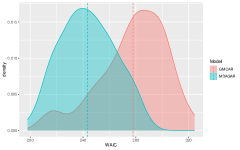
(a) WAIC: low

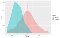
(b) WAIC: medium

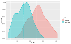
(c) WAIC: high

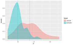
(d) Score $D$: low

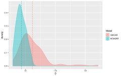
(e) Score $D$: medium

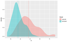
(f) Score $D$: high

Figure 1: Density plots for WAICs and $D$ scores over 85 datasets. Density plots of WAIC for MDAGAR (blue) and GMCAR (red) models with low, medium and high correlation are shown in (a), (b) and (c) respectively, while (d)–(f) are the corresponding density plots for $D$ scores. The dotted vertical line shows the mean for WAIC and D in each plot.

Figure 2 presents scatter plots for the true values (x axis) of spatial random effects against their posterior estimates (y axis). To be precise, each panel plots $85\times 48\times 2=8160$ true values of the elements of the $96\times 1$ vector $\bm{w}$ for $85$ datasets against their corresponding posterior estimates. We see strong agreements between the true values and their estimates for both MDAGAR and GMCAR. The agreement is more pronounced for the datasets corresponding to medium and high correlations. For the low-correlation datasets, the agreement is clearly weaker although MDAGAR does slightly better than GMCAR.

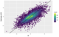
(a) MDAGAR: low

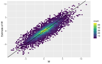
(b) MDAGAR: medium

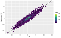
(c) MDAGAR: high

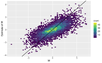
(d) GMCAR: low

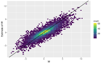
(e) GMCAR: medium

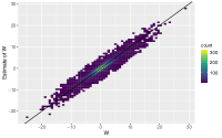
(f) GMCAR: high

Figure 2: Scatter plots for estimates of spatial random effects (y axis) against the true values (x axis) with $45^{\circ}$ lines over 85 datasets: (a)–(c) are estimates from MDAGAR model with low, medium and high correlation, while (d)–(f) are the corresponding estimates from GMCAR.

We compute $\displaystyle D_{KL}(N(\bm{0},\bm{Q}_{true})||N(\bm{0},\bm{Q}_{w}))=\frac{1}{2}\left[\log\left(\frac{\det(\bm{Q}_{true})}{\det(\bm{Q}_{w})}\right)+\mbox{tr}(\bm{Q}_{w}\bm{Q}_{true}^{-1})-qk\right]$, which is the Kullback-Leibler Divergence between the model for $\bm{w}$ with the true generative precision matrix ($\bm{Q}_{true}$) and those with MDAGAR and GMCAR precisions ($\bm{Q}_{w}$). Using the posterior samples in the precision matrix, we evaluate the posterior probability that $D_{KL}(N(\bm{0},\bm{Q}_{true})||N(\bm{0},\bm{Q}_{MDAGAR}))$ is smaller than $D_{KL}(N(\bm{0},\bm{Q}_{true})||N(\bm{0},\bm{Q}_{w}))$. Figure S.5 depicts a density plot of these probabilities over the 85 data sets. When correlations are low and medium, the MDAGAR has a mean probability of around $69\%$ to be closer to the true model than the GMCAR, while for high correlations GMCAR excels with an average probability of $72\%$ to be closer to the true model. These findings are consistent with the results of AMSE, where the GMCAR tended to perform better when the correlations are high. Additional comparative diagnostics from MDAGAR and GMCAR such as coverage probabilities for parameters and correlation between random effects for two diseases in the same state are presented in S.7.2.

3.3 Model selection for different disease orders

We now evaluate the effectiveness of the method in Section 2.5 at selecting the model with the correct ordering of diseases. We used the bridgesampling package in R to compute $p(M_{i}\,|\,\bm{y}^{(n)})=\mbox{max}_{t=1,\ldots,6}\ p(M_{t}\,|\,\bm{y}^{(n)})$ for each of $n=50\times 6$ data sets generated as described in Section 3.1. Table 1 presents the probability of each model being selected for different true model scenarios. The probability of selecting the true model is shown in bold along the diagonal. Our experiment reveals that bridge sampling is extremely effective at choosing the correct order. It was able to identify the correct order between $80\%$ to $90\%$, which is substantially larger than any of the probability of choosing any of the misspecified models.

Table 1: Proportion of times ($\pi(M_{i})$) bridge sampling chose the model with the correct order out of the 50 data sets with that order.

True model	$\pi(M_{1})$	$\pi(M_{2})$	$\pi(M_{3})$	$\pi(M_{4})$	$\pi(M_{5})$	$\pi(M_{6})$
$M_{1}$	0.90	0.00	0.10	0.00	0.00	0.00
$M_{2}$	0.00	0.86	0.00	0.00	0.14	0.00
$M_{3}$	0.14	0.00	0.86	0.00	0.00	0.00
$M_{4}$	0.00	0.00	0.00	0.90	0.00	0.10
$M_{5}$	0.00	0.22	0.00	0.00	0.78	0.00
$M_{6}$	0.00	0.00	0.00	0.16	0.00	0.84

4 Multiple Cancer Analysis from SEER

We now turn to an areal dataset with 4 different cancers using the MDAGAR model. The data set is extracted from the SEER^∗Stat database using the SEER^∗Stat statistical software (National Cancer Institute, 2019). The dataset consists of four cancers: lung, esophagus, larynx and colorectal, where the outcome is the 5-year average age-adjusted incidence rates (age-adjusted to the 2000 U.S. Standard Population) per 100,000 population in the years from 2012 to 2016 across 58 counties in California, USA, as mapped in Figure 6(a). The maps exhibit preliminary evidence of correlation across space and among cancers. Cutoffs for the different levels of incidence rates are quantiles for each cancer. For all four cancers, incidence rates are relatively higher in counties concentrated in the middle northern areas including Shasta, Tehama, Glenn, Butte and Yuba than those other areas. In general, northern areas have higher incidence rates than in the southern part. This is especially pronounced for lung cancer and esphogus cancer. For larynx cancer, in spite of the highest incidence rate concentrated in the north, the incidence rates in the south are mostly at the same high level. For colorectal cancer, the edge areas at the bottom also exhibit high incidence rates.

Overall, counties with similar levels of incidence rates tend to depict some spatial clustering. We analyze this data set using (2.4.1) with the following prior specification

$$p(\bm{\eta},\bm{\rho},\bm{\tau},\bm{\sigma},\bm{w}) =\prod_{i=1}^{q}Unif(\rho_{i}\,|\,0,1)\times\prod_{i=2}^{q}\prod_{j=1}^{i-1}N(\bm{\eta}_{ij}\,|\,0,0.01\bm{I}_{2})\times\prod_{i=1}^{q}N(\bm{\beta}_{i}\,|\,0,0.001\bm{I})$$

$$\times\prod_{i=1}^{q}IG(1/\tau_{i}\,|\,2,0.1)\times\prod_{i=1}^{q}IG(\sigma_{i}^{2}\,|\,2,1)\times N(\bm{w}\,|\,\bm{0},\bm{Q_{w}})\;.$$ (19)

We also discuss a case excluding the risk factor (see Section S.8).

For covariates, we include county attributes that possibly affect the incidence rates, including percentages of residents younger than 18 years old (young_ij), older than 65 years old (old_ij), with education level below high school (edu_ij), percentages of unemployed residents (unemp_ij), black residents (black_ij), male residents (male_ij), uninsured residents (uninsure_ij), and percentages of families below the poverty threshold (poverty_ij). All covariates are common for different cancers and extracted from the SEER^∗Stat database (National Cancer Institute, 2019) for the same period, 2012 - 2016. Since cigarette smoking is a common risk factor for cancers, adult smoking rates (smoke_ij) for 2014–2016 were obtained from the California Tobacco Facts and Figures 2018 database (California Department of Public Health, 2018). Spatial patterns in the map of adult cigarette smoking rates, shown in Figure 6(b), are similar to the incidence of cancers, especially lung and esophageal cancers, the highest smoking rates are concentrated in the north. While some central California counties (e.g., Stanislaus, Tuolumne, Merced, Mariposa, Fresno and Tulare) also exhibit high rates, although there is clearly less spatial clustering of the high rates than in the north.

Since the order of cancers in the DAG specify the model, we fit all $4!=24$ models using (2.4.1) and compute the marginal likelihoods using bridge sampling (Section  2.5). By setting the prior model probabilities as $p(M=M_{t})=\frac{1}{24}$ for $t=1,2,\ldots,24$, we compute the posterior model probabilities using (11). These are presented in Table S.5. We obtain Bayesian model averaged (BMA) estimates using (16) with the weights in Table S.5. Among all models, model $M_{10}$ is selected as the best model with the largest posterior probability $0.577$ and the corresponding conditional structure is $[\mbox{esophageal}]\times[\mbox{larynx}\,|\,\mbox{esophageal}]\times[\mbox{colorectal}\,|\,\mbox{esophageal},\mbox{larynx}]\times[\mbox{lung}\,|\,\mbox{esophageal},\mbox{larynx},\mbox{colorectal}]$.

Table 2 is a summary of the parameter estimates including regression coefficients, spatial autocorrelation ($\rho_{i}$), spatial precision ($\tau_{i}$) and noise variance ($\sigma_{i}^{2}$) for each cancer. From $M_{10}$ and BMA, we find the regression slopes for the percentage of smokers and uninsured residents are significantly positive and negative, respectively, for esophageal cancer. The negative association between percentage of uninsured and esophageal cancer may seem surprising, but is likely a consequence of spatial confounding with counties exhibiting low incidence rates for esophageal cancer having a relatively large number of uninsured residents (see top right in 6(a) and the right most figure in 6(b)). Since esophageal cancer has low incidence rates, this association could well be spurious due to spatial confounding. Percentage of smokers is, unsurprisingly, found to be a significant risk factor for lung cancer, while the percentage of blacks seems to be significantly associated with elevated incidence of larynx cancer. In addition, we tend to see that percentage of population below the poverty level has a pronounced association with higher rates of lung and esophageal cancer.

Recall from Section 2.4 that $\rho_{1}$ is the residual spatial autocorrelation for esophageal cancer after accounting for the explanatory variables, while $\rho_{i}$ for $i=2,3,4$ are residual spatial autocorrelations after accounting for the explanatory variables and the preceding cancers in the model $M_{10}$. From Table 2 we see that esophageal cancer exihibits relatively weaker spatial autocorrelation, while the residual spatial autocorrelations for larynx and colorectal cancers after accounting for preceding cancers are both at moderate levels of around 0.5. Similarly for the spatial precision $\tau_{i}$, larynx appears to have the smallest conditional variability while that for colorectal and lung are slightly larger.

Table 2: Posterior means (95$\%$ credible intervals) for parameters estimated from $M_{10}$ and BMA estimates for regression coefficients only for the SEER four cancer dataset.

Parameters	Model	Esophageal	Larynx	Colorectal	Lung
Intercept	$M_{10}$	16.76 (4.06, 29.56)	6.37 (-1.16, 13.89)	19.16 (-11.94, 49.72)	28.68 (-18.3, 74.93)
	BMA	15.87 (2.92, 28.63)	6.85 (-0.71, 14.38)	18.21 (-14.03, 49.07)	28.25 (-18.12, 74.52)
Smokers ($\%$)	$M_{10}$	0.25 (0.12, 0.37)	0.04 (-0.03, 0.12)	0.23 (-0.12, 0.57)	0.81 (0.08, 1.62)
	BMA	0.23 (0.10, 0.36)	0.05 (-0.03, 0.12)	0.22 (-0.13, 0.58)	0.80 (0.08, 1.59)
Young ($\%$)	$M_{10}$	-0.12 (-0.31, 0.07)	-0.07 (-0.18, 0.04)	0.27 (-0.2, 0.76)	-0.08 (-0.90, 0.74)
	BMA	-0.11 (-0.3, 0.08)	-0.08 (-0.19, 0.03)	0.29 (-0.18, 0.78)	-0.01 (-0.86, 0.82)
Old ($\%$)	$M_{10}$	-0.11 (-0.25, 0.04)	-0.05 (-0.14, 0.03)	0.10 (-0.28, 0.48)	-0.09 (-0.81, 0.67)
	BMA	-0.10 (-0.25, 0.05)	-0.05 (-0.14, 0.03)	0.10 (-0.29, 0.49)	-0.08 (-0.79, 0.66)
Edu ($\%$)	$M_{10}$	0.02 (-0.08, 0.12)	-0.02 (-0.08, 0.04)	0.16 (-0.12, 0.43)	-0.20 (-0.75, 0.31)
	BMA	0.02 (-0.09, 0.12)	-0.02 (-0.07, 0.04)	0.15 (-0.14, 0.42)	-0.24 (-0.79, 0.27)
Unemp ($\%$)	$M_{10}$	-0.13 (-0.29, 0.03)	0.01 (-0.08, 0.10)	-0.09 (-0.54, 0.37)	0.60 (-0.47, 1.55)
	BMA	-0.12 (-0.28, 0.05)	0.01 (-0.08, 0.1)	-0.08 (-0.54, 0.38)	0.61 (-0.43, 1.56)
Black ($\%$)	$M_{10}$	0.14 (-0.06, 0.34)	0.14 (0.03, 0.26)	-0.16 (-0.73, 0.39)	0.15 (-1.06, 1.29)
	BMA	0.13 (-0.07, 0.33)	0.15 (0.03, 0.27)	-0.18 (-0.75, 0.39)	0.14 (-1.02, 1.25)
Male ($\%$)	$M_{10}$	-0.04 (-0.17, 0.09)	0.00 (-0.07, 0.08)	0.24 (-0.12, 0.60)	0.14 (-0.57, 0.79)
	BMA	-0.04 (-0.17, 0.09)	0 (-0.07, 0.08)	0.24 (-0.12, 0.62)	0.14 (-0.55, 0.82)
Uninsured ($\%$)	$M_{10}$	-0.24 (-0.44, -0.04)	-0.08 (-0.20, 0.04)	0.07 (-0.44, 0.58)	0.01 (-0.82, 0.86)
	BMA	-0.23 (-0.42, -0.02)	-0.08 (-0.2, 0.04)	0.09 (-0.42, 0.61)	0 (-0.81, 0.82)
Poverty ($\%$)	$M_{10}$	0.30 (-0.24, 0.84)	0.20 (-0.12, 0.51)	-0.06 (-1.51, 1.45)	0.85 (-2.15, 3.85)
	BMA	0.32 (-0.23, 0.87)	0.2 (-0.12, 0.51)	-0.08 (-1.54, 1.42)	0.8 (-2.14, 3.75)
$\rho_{i}$	$M_{10}$	0.25 (0.01, 1.00)	0.33 (0.01, 0.96)	0.50 (0.03, 0.97)	0.52 (0.03, 0.99)
$\tau_{i}$	$M_{10}$	25.27 (5.08, 61.57)	27.60 (8.05, 60.42)	19.97 (3.06, 55.61)	20.31 (1.77, 55.92)
$\sigma_{i}^{2}$	$M_{10}$	1.67 (1.11, 2.47)	0.49 (0.28, 0.75)	8.22 (1.09, 14.23)	1.19 (0.18, 5.21)

For the posterior mean incidence rates and spatial random effects $w_{ij}$, we present estimates from model $M_{10}$ and BMA. Figure 3(a) and 3(b) are maps of posterior mean spatial random effects and model fitted incidence rates for four cancers obtained from BMA, while Figure 3(c) and 3(d) show maps of those from model $M_{10}$. The posterior mean incidence rates from BMA and $M_{10}$ are in accord with each other, and both present DAGAR-smoothed versions of the original patterns in Figure 6(a). For posterior means of spatial random effects, in general, the estimates from $M_{10}$ are similar to model averaged estimates, especially for lung and colorectal cancers, exhibiting relatively large positive values in the northern counties, where the incidence rates are high. However, for esophageal and larynx cancers we see slight discrepancies between $M_{10}$ and BMA in the north. The BMA estimates produce larger positive random effects, ranging between $0.1-0.5$, in most counties, while $M_{10}$ produces estimates between $0-0.1$ for esophageal cancer. More counties with random effects larger than $0.1$ are estimated from $M_{10}$ for larynx cancer. We believe this is attributable, at least in part, to another competitive model, $M_{15}=[\mbox{larynx}]\times[\mbox{esophagus}\,|\,\mbox{larynx}]\times[\mbox{lung}\,|\,\mbox{larynx},\mbox{esophagus}]\times[\mbox{colorectal}\,|\,\mbox{larynx},\mbox{esophagus},\mbox{lung}]$ (posterior probability $0.342$), which contributes to the BMA. On the other hand, the effects of some important county-level covariates play an essential role in the discrepancy between the estimates of random effects and model fitted incidence rates for each cancer.

Recall from Section 2 that $\eta_{0ii^{\prime}}$ and $\eta_{1ii^{\prime}}$ reflect the associations among cancers that can be attributed to spatial structure. Specifically, larger values of $\eta_{0ii^{\prime}}$ will indicate inherent associations unrelated to spatial structure, while the magnitude of $\eta_{1ii^{\prime}}$ reflects associations due to spatial structure. Figure S.7 presents posterior distributions of $\bm{\eta}$ for all pairs of cancers. We see from the distribution of $\eta_{043}$ that there is a pronounced non-spatial component in the association between lung and colorectal cancers. Similar, albeit somewhat less pronounced, non-spatial associations are seen between larynx and esophageal cancers and between lung and larynx cancers. Analogously, the posterior distributions for $\eta_{143}$ and $\eta_{132}$ tend to have substantial positive support suggesting substantial spatial cross-correlations between lung and colorectal cancers and between colorectal and larynx cancers. Interestingly, we find negative support in the posterior distributions for $\eta_{121}$ and $\eta_{142}$. The negative mass implies that the covariance among cancers within a region is suppressed by strong dependence with neighboring regions. This seems to be the case for associations between lung and esophageal cancers and between lung and larynx cancers.

We also present supplementary analysis that excludes adult smoking rates from the covariates, which we refer to as “Case 2”. Figure S.8 shows estimated correlations between pairwise cancers in each of the 58 counties. The top row presents the correlations including smoking rates (“Case 1”) as has been analyzed here. The bottom row presents the corresponding maps for “Case 2”. Interestingly, accounting for smoking rates substantially diminishes the associations among esophageal, colorectal and lung cancers. These are significantly associated in “Case 2” but only lung and colorectal retain their significance after accounting for smoking rates.

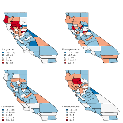
(a) BMA: posterior mean spatial random effects

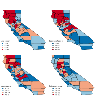
(b) BMA: posterior mean incidence rates

(c) $M_{10}$: posterior mean spatial random effects

(d) $M_{10}$: posterior mean incidence rates

Figure 3: Maps of posterior results using BMA and the highest probabilty model $M_{10}$ for lung, esophagus, larynx and colorectal cancer in California including posterior mean spatial random effects and posterior mean incidence rates as shown in (a) (b) for BMA and (c) (d) for $M_{10}$;

5 Discussion

We have developed a conditional multivariate “MDAGAR” model to estimate spatial correlations for multiple correlated diseases based on a currently proposed class of DAGAR models for univariate disease mapping, as well as providing better interpretation of the association among diseases. We demonstrate that MDAGAR tends to outperform GMCAR when association between spatial random effects for different diseases is weak or moderate. Inference is competitive when associations are strong. MDAGAR retains the interpretability of spatial autocorrelations, as in univariate DAGAR, separating the spatial correlation for each disease from any inherent or endemic association among diseases. While MDAGAR, like all DAG based models, is specified according to a fixed order of the diseases, we show that a bridge sampling algorithm can effectively choose among the different orders and also provide Bayesian model averaged inference in a computationally efficient manner.

Our data analysis reveals that correlations between incidence rates for different cancers are impacted by covariates. For example, eliminating adult cigarette smoking rates produces similar spatial patterns for the incidence rates of esophageal, lung and colorectal cancer. In addition, the significant correlation between lung and esophageal cancer, even after accounting for smoking rates, implies other inherent or endemic association such as latent risk factors and metabolic mechanisms. We also see that the MDAGAR based posterior estimates of the latent spatial effects in Figure 3(a) and 3(c) resemble those from an MDAGAR without covariates (Figure S.9), while the maps for the estimated incidence rates in Figure 3(b) and 3(d) account for the spatial variability of the covariates.

Future challenges will include scalability with very large number of diseases because, as we have seen, the number of models to be fitted grows exponentially with the number of diseases. One way to obviate this issue is to adopt a joint modeling approach analogous to order-free MCAR models (Jin et al., 2007) that build rich spatial structures from linear transformations of simpler latent variables. For instance, we can develop alternate MDAGAR models by specifying $\bm{w}=\bm{\Lambda}\bm{f}$, where $\bm{\Lambda}$ is a suitably specified matrix and $\bm{f}$ is a latent vector whose components follow independent univariate DAGAR distributions. This will avoid the order dependence, but the issue of identifying and specifying $\bm{\Lambda}$ will need to be considered as will the interpretation of disease specific spatial autocorrelations.

Supplementary Materials

The R code implementing our models are available at https://github.com/LeiwenG/Multivariate_DAGAR.

S.6 Algorithm for Model Implementation

We outline model implementation for (2.4.1) using Markov Chain Monte Carlo (MCMC). We update $\{\bm{w},\bm{\beta},\bm{\sigma},\bm{\tau},\bm{\eta}_{2},\dots,\bm{\eta}_{q}\}$ using Gibbs steps, while the elements of $\bm{\rho}$ are updated from their full conditional distributions using Metropolis random walk steps (Robert and Casella, 2004). A particularly appealing feature of our proposed MDAGAR model is that the spatial weight parameters $\bm{\eta}=\{\bm{\eta}_{2},\dots,\bm{\eta}_{q}\}$ render Gaussian full conditional distributions in addition to the customary Gaussian full conditional distributions for $\bm{\beta}$ and $\bm{w}$. As a matter of notational convenience for the derivations that follow, we use $N(\bm{\mu},\bm{V})$ to denote the normal distribution with variance-covariance matrix $\bm{V}$. This difference from our notation in the main manuscript where we use the precision matrix in the argument of normal distribution.

S.6.1 Full Conditional Distributions

The full conditional distribution for each $\bm{\beta}_{i}$ is

$$\bm{\beta}_{i}|\bm{y}_{i},\bm{w}_{i},\sigma_{i}^{2}\sim N(\bm{M}_{i}\bm{m}_{i},\bm{M}_{i})$$ (S.20)

where $\bm{M}_{i}=\left(\frac{1}{\sigma_{i}^{2}}\bm{X}_{i}^{\top}\bm{X}_{i}+\frac{1}{\sigma_{\beta}^{2}}\bm{I}_{p_{i}}\right)^{-1}$ and $\bm{m}_{i}=\frac{1}{\sigma_{i}^{2}}\bm{X}_{i}^{\top}\left(\bm{y}_{i}-\bm{w}_{i}\right)$. Similarly, the full conditional distribution of each $\sigma_{i}^{2}$ follows an inverse gamma distribution,

$$\sigma_{i}^{2}|\bm{y}_{i},\bm{\beta}_{i},\bm{w}_{i}\sim IG\left(a_{\sigma}+\frac{k}{2},b_{\sigma}+\frac{1}{2}\left(\bm{y}_{i}-\bm{X}_{i}\bm{\beta}_{i}-\bm{w}_{i}\right)^{\top}\left(\bm{y}_{i}-\bm{X}_{i}\bm{\beta}_{i}-\bm{w}_{i}\right)\right).$$ (S.21)

The full conditional distribution for $\bm{w}_{i}$ for each $i=2,\dots,q-1$ is

$$p\left(\bm{w}_{i}\,|\,\bm{w}_{1},\dots,\bm{w}_{i-1},\bm{w}_{i+1},\bm{w}_{i+1},\dots,\bm{w}_{q},\bm{y}_{i},\bm{\beta}_{i},\sigma_{i}^{2},\bm{\eta}_{i},\dots,\bm{\eta}_{q},\rho_{i},\dots,\rho_{q},\tau_{i},\dots,\tau_{q}\right)$$

$$\quad\quad\quad\quad\quad\propto\prod_{n=i}^{q}\exp{\left\{-\frac{\tau_{n}}{2}\left(\bm{w}_{n}-\sum_{i^{\prime}=1}^{n-1}\bm{A}_{ni^{\prime}}\bm{w}_{i^{\prime}}\right)^{\top}\bm{Q}\left(\rho_{n}\right)\left(\bm{w}_{n}-\sum_{i^{\prime}=1}^{n-1}\bm{A}_{ni^{\prime}}\bm{w}_{i^{\prime}}\right)\right\}}$$

$$\quad\quad\quad\quad\quad\quad\quad\quad\quad\times\exp{\left\{-\frac{1}{2\sigma_{i}^{2}}\left(\bm{y}_{i}-\bm{X}_{i}\bm{\beta}_{i}-\bm{w}_{i}\right)^{\top}\left(\bm{y}_{i}-\bm{X}_{i}\bm{\beta}_{i}-\bm{w}_{i}\right)\right\}}$$ (S.22)

which is equal to $N(\bm{w}_{i}\,|\,\bm{G}_{i}\bm{g}_{i},\bm{G}_{i})$, where

$$\bm{G}_{i}=\bigg{[}\tau_{i}\bm{Q}(\rho_{i})+\sum_{n=i+1}^{q}\tau_{n}\bm{A}_{ni}^{\top}\bm{Q}(\rho_{n})\bm{A}_{ni}+\frac{1}{\sigma_{i}^{2}}\bm{I}_{k}\bigg{]}^{-1}$$

and $\displaystyle\bm{g}_{i}=\tau_{i}\bm{Q}(\rho_{i})\sum_{n=1}^{i-1}\bm{A}_{in}\bm{w}_{n}+\sum_{n=i+1}^{q}\tau_{n}\bm{A}_{ni}^{\top}\bm{Q}(\rho_{n})\left(\bm{w}_{n}-\sum_{i^{\prime}=1,i^{\prime}\neq i}^{n-1}\bm{A}_{ni^{\prime}}\bm{w}_{i^{\prime}}\right)+\frac{1}{\sigma_{i}^{2}}(\bm{y}_{i}-\bm{X}_{i}\bm{\beta}_{i})$. For $i=1$ and $q$, we have

$$\bm{w}_{1}|\bm{w}_{2},\dots,\bm{w}_{q},\bm{y}_{1},\bm{\beta}_{1},\sigma_{1}^{2},\bm{\eta},\bm{\rho},\bm{\tau} \sim N(\bm{G}_{1}\bm{g}_{1},\bm{G}_{1})$$

$$\bm{w}_{q}|\bm{w}_{1},\dots,\bm{w}_{q-1},\bm{y}_{q},\bm{\beta}_{q},\sigma_{1}^{2},\bm{\eta}_{q},\rho_{q},\tau_{q} \sim N(\bm{G}_{q}\bm{g}_{q},\bm{G}_{q})$$

, where

$$\bm{G}_{1} =\left(\tau_{1}\bm{Q}(\rho_{1})+\sum_{n=2}^{q}\tau_{n}\bm{A}_{n1}^{\top}\bm{Q}(\rho_{n})\bm{A}_{n1}+\frac{1}{\sigma_{1}^{2}}\bm{I}_{k}\right)^{-1},$$

$$\bm{g}_{1} =\tau_{2}\bm{A}_{21}^{\top}\bm{Q}(\rho_{2})\bm{w}_{2}+\sum_{n=3}^{q}\tau_{n}\bm{A}_{n1}^{\top}\bm{Q}(\rho_{n})\left(\bm{w}_{n}-\sum_{i^{\prime}=2}^{n-1}\bm{A}_{ni^{\prime}}\bm{w}_{i^{\prime}}\right)+\frac{1}{\sigma_{1}^{2}}(\bm{y}_{1}-\bm{X}_{1}\bm{\beta}_{1}),$$

$$\bm{G}_{q} =\left(\tau_{q}\bm{Q}(\rho_{q})+\frac{1}{\sigma_{q}^{2}}\bm{I}_{k}\right)^{-1}$$

$$\bm{g}_{q} =\tau_{q}\bm{Q}(\rho_{q})\sum_{n=1}^{q-1}\bm{A}_{qn}\bm{w}_{n}+\frac{1}{\sigma_{q}^{2}}(\bm{y}_{q}-\bm{X}_{q}\bm{\beta}_{q}).$$

The full conditional distribution of each $\tau_{i}$ is

$$\tau_{1}|\bm{w}_{1},\rho_{1}\sim G\left(a_{\tau_{1}}+\frac{k}{2},b_{\tau_{1}}+\frac{1}{2}\bm{w}_{1}^{T}\bm{Q}(\rho_{1})\bm{w}_{1}\right),\\ \tau_{i}|\bm{w}_{1},\dots,\bm{w}_{i},\bm{\eta}_{i},\rho_{i}\sim G\left(a_{\tau_{i}}+\frac{k}{2},b_{\tau_{i}}+\frac{1}{2}\left(\bm{w}_{i}-\sum_{i^{\prime}=1}^{i-1}\bm{A}_{i,i^{\prime}}\bm{w}_{i^{\prime}}\right)^{\top}\bm{Q}(\rho_{i})\left(\bm{w}_{i}-\sum_{i^{\prime}=1}^{i-1}\bm{A}_{i,i^{\prime}}\bm{w}_{i^{\prime}}\right)\right),\\ i=2,3,\dots,q$$ (S.23)

We now derive the full conditional distributions for the $\bm{\eta}_{i}$s. From (7) with $i=2$, each element in $\bm{w}_{2}$ can be written as $w_{2j}=\eta_{021}w_{1j}+\eta_{121}\sum_{j^{\prime}\sim j}w_{1j^{\prime}}+\epsilon_{2j}$, where $\epsilon_{2j}$ is the $j$th element in $\bm{\epsilon}_{2}$. To extract $\bm{\eta}_{21}=(\eta_{021},\eta_{121})^{\top}$ from the matrix $\bm{A}_{21}$, $\bm{A}_{21}\bm{w}_{1}$ is rewritten as $\bm{Z}_{1}\bm{\eta}_{21}$ where $\bm{Z}_{1}=(\bm{w}_{1},\bm{\zeta}_{1})$ and $\bm{\zeta}_{1}=\left(\sum_{j^{\prime}\sim 1}w_{1j^{\prime}},\dots,\sum_{j^{\prime}\sim k}w_{1j^{\prime}}\right)^{\top}$. In general, $\bm{A}_{ii^{\prime}}\bm{w}_{i^{\prime}}=\bm{Z}_{i^{\prime}}\bm{\eta}_{ii^{\prime}}$ with $\bm{Z}_{i^{\prime}}=(\bm{w}_{i^{\prime}},\bm{\zeta}_{i^{\prime}})$, where $\bm{\zeta}_{i^{\prime}}=\left(\sum_{j^{\prime}\sim 1}w_{i^{\prime}j^{\prime}},\dots,\sum_{j^{\prime}\sim k}w_{i^{\prime}j^{\prime}}\right)^{\top}$. Consequently, (5) can be written as $\bm{w}_{i}=\bm{\delta}_{i}\bm{\eta}_{i}+\bm{\epsilon}_{i}$, where block matrix $\bm{\delta}_{i}=(\bm{Z}_{1},\dots,\bm{Z}_{i-1})$. If $\bm{\eta}_{i}\sim N(\bm{\mu}_{i},\bm{V}_{i})$, then the full conditional distribution of $\bm{\eta}_{i}$ is

$$p(\bm{\eta}_{i}\,|\,\bm{w}_{1},\dots,\bm{w}_{i},\rho_{i}) \propto\exp{\left\{-\frac{\tau_{i}}{2}(\bm{w}_{i}-\bm{\delta}_{i}\bm{\eta}_{i})^{\top}\bm{Q}(\rho_{i})(\bm{w}_{i}-\bm{\delta}_{i}\bm{\eta}_{i})\right\}}$$

$$\quad\quad\quad\times\exp{\left\{-\frac{1}{2}(\bm{\eta}_{i}-\bm{\mu}_{i})^{\top}\bm{V}_{i}^{-1}(\bm{\eta}_{i}-\bm{\mu}_{i})\right\}}.$$ (S.24)

The above is equal to $N(\bm{\eta}_{i}\,|\,\bm{H}_{i}\bm{h}_{i},\bm{H}_{i})$, where $\bm{H}_{i}=\left(\tau_{i}\bm{\delta}_{i}^{\top}\bm{Q}(\rho_{i})\bm{\delta}_{i}+\bm{V}_{i}^{-1}\right)^{-1}$ and $\bm{h}_{i}=\tau_{i}\bm{\delta}_{i}^{\top}\bm{Q}(\rho_{i})\bm{w}_{i}+\bm{V}_{i}^{-1}\bm{\mu}_{i}$. For our analysis we set $\bm{\mu}_{i}=\bm{0}$ and $\bm{V}_{i}=1000\bm{I}$.

S.6.2 Metropolis within Gibbs

Let $\gamma_{i}=\log(\frac{\rho_{i}}{1-\rho_{i}})$, $\gamma_{i}\in\mathbb{R}$ and $\bm{\gamma}=(\gamma_{1},\dots,\gamma_{q})^{\top}$. The full conditional distribution of $\bm{\gamma}$ is

$$p(\bm{\gamma}|\bm{w},\bm{\eta}_{2},\dots,\bm{\eta}_{q},\bm{\tau})\propto p(\bm{w}|\bm{\tau},\bm{\eta}_{2},\dots,\bm{\eta}_{q},\bm{\rho})\times p(\bm{\rho})|J|,$$ (S.25)

where $p(\bm{w}|\bm{\tau},\bm{\eta}_{2},\dots,\bm{\eta}_{q},\bm{\rho})=N(\bm{w}\,|\,\bm{G}\bm{g},\bm{G})$, $\bm{G}=\left(\bm{Q}_{w}+\bm{\Sigma}^{-1}\right)^{-1}$, $\bm{g}=\bm{\Sigma}^{-1}\left(\bm{y}-\bm{X}\bm{\beta}\right)$, $\bm{\Sigma}=diag(\bm{\sigma})\otimes\bm{I}_{k}$ and $J=\prod_{i=1}^{q}\rho_{i}(1-\rho_{i})$. Using the formula of transformation, $p(\bm{\rho})|J|$ is the prior for $\bm{\gamma}$ and in the right-hand side, $\bm{\rho}$ can be substituted by $\bm{\gamma}$ given $\rho_{i}=\frac{e^{\gamma_{i}}}{1+e^{\gamma_{i}}}$.

In our analysis, for each model we ran two MCMC chains for 30,000 iterations each. Posterior inference was based upon 15,000 samples retained after adequate convergence was diagnosed. The MDAGAR model in the simulation examples was programmed in the S language as implemented in the R statistical computing environment. All other models were implemented using the rjags package available from CRAN https://cran.r-project.org/web/packages/rjags/.

S.7 Supplementary Details in Simulation

S.7.1 WAIC, AMSE and D score

For the simulation studies in Section 3.2, let $\bm{\theta}=\{\bm{\beta},\bm{\sigma},\bm{w}\}$. The likelihood of each data point $p(y_{ij}\mid\bm{\theta})=p\left(y_{ij}\mid\bm{x}_{ij}^{\top}\bm{\beta}_{i}+w_{ij},1/\sigma_{i}^{2}\right)$ is needed for calculating WAIC which is defined as

$$WAIC=-2\left(\widehat{lpd}-\hat{p}_{WAIC}\right)\;,$$

where $\widehat{lpd}$ is computed using posterior samples as the sum of log average predictive density i.e. $\sum_{i=1}^{q}\sum_{j=1}^{k}\log\left(\frac{1}{L}\sum_{\ell=1}^{L}p\left(y_{ij}\mid\bm{\theta}^{(\ell)}\right)\right)$, $\bm{\theta}^{(\ell)}$ for $\ell=1,\dots,L$ being $L$ posterior samples of $\bm{\theta}$, and $\hat{p}_{WAIC}$ is the estimated effective number of parameters computed as

$$\sum_{i=1}^{q}\sum_{j=1}^{k}V_{\ell=1}^{L}\left(\log p\left(y_{ij}\mid\bm{\theta}^{(\ell)}\right)\right)$$

with $V_{\ell=1}^{L}\left(\log p\left(y_{ij}\mid\bm{\theta}^{(\ell)}\right)\right)=\frac{1}{L-1}\sum_{\ell=1}^{L}\left[\log p\left(y_{ij}\mid\bm{\theta}^{(\ell)}\right)-\frac{1}{L}\sum_{\ell=1}^{L}\log p\left(y_{ij}\mid\bm{\theta}^{(\ell)}\right)\right]^{2}$.

Turning to the $D$ score, we draw replicates $y_{ij}$, $y_{\text{rep},ij}^{(\ell)}\sim N(\bm{x}_{ij}^{\top}\bm{\beta}_{i}^{(\ell)}+w_{ij}^{(\ell)},1/\sigma_{i}^{2(\ell)})$ and compute $D=G+P$. Here $G=\sum_{i=1}^{q}||\bm{y}_{i}-\bar{\bm{y}}_{\text{rep},i}||^{2}$ is a goodness-of-fit measure, where $\bar{\bm{y}}_{\text{rep},i}$ is the mean veactor with elements $\bar{y}_{\text{rep},ij}=\frac{1}{L}\sum_{\ell=1}^{L}y_{\text{rep},ij}^{(\ell)}$ and $P=\sum_{i=1}^{q}\sum_{j=1}^{k}\sigma_{\text{rep},ij}^{2}$ is a summary of variance, where $\sigma_{\text{rep},ij}^{2}$ is the variance of $y_{\text{rep},ij}^{(\ell)}$ for $\ell=1,\ldots,L$.

For AMSE, we use $w_{ij}$ as the true value of each random effect and $\hat{w}_{ij}^{(n)}$ is the posterior mean of $w_{ij}$ for the data set $n$. The estimated AMSE is calculated as $\widehat{AMSE}=\frac{1}{Nqk}\sum_{n=1}^{N}\sum_{i=1}^{q}\sum_{j=1}^{k}\left(\hat{w}_{ij}^{(n)}-w_{ij}\right)^{2}$ with associated Monte Carlo standard error estimate

$$\widehat{SE}(\widehat{AMSE})=\sqrt{\frac{1}{(Nqk)(Nqk-1)}\sum_{n=1}^{N}\sum_{i=1}^{q}\sum_{j=1}^{k}\left[\left(\hat{w}_{ij}^{(n)}-w_{ij}\right)^{2}-\widehat{AMSE}\right]^{2}}.$$

S.7.2 Coverage Probability

For the simulation studies in Section 3.2, Table S.3 shows the coverage probabilities (CP) defined as the mean coverage for a parameter by the $95\%$ credible intervals over 85 datasets. The MDAGAR offers satisfactory coverages for all parameters when correlations are low and medium, outperforming GMCAR, while GMCAR presents competitive performance with MDAGAR for high correlations. Figure S.4 plots coverage probabilities of correlation between two diseases in the same region, given by $corr(w_{1j},w_{2j})=cov(w_{1j},w_{2j})/(\surd var(w_{1j})\surd var(w_{2j}))$, for MDAGAR and GMCAR. Let $\bm{Q}(\rho_{i})^{-1}=\{d_{ijj^{\prime}}\}$, we obtain $cov(w_{1j},w_{2j})=\tau_{1}^{-1}(\eta_{021}d_{1jj}+\eta_{121}\sum_{j^{\prime}\sim j}d_{1jj^{\prime}})$, $var(w_{1j})=\tau_{1}^{-1}d_{1jj}$ and

$$var(w_{2j})=\tau_{1}^{-1}[\eta_{021}(\eta_{021}d_{1jj}+\eta_{121}\sum_{j^{\prime}\sim j}d_{1jj^{\prime}})+\eta_{121}\sum_{j^{\prime}\sim j}(\eta_{021}d_{1jj^{\prime}}+\eta_{121}\sum_{j^{\prime\prime}\sim j}d_{1j^{\prime\prime}j^{\prime}})]+\tau_{2}^{-1}d_{2jj}.$$

The MDAGAR performs better in estimating disease correlations in the same region for all scenarios, especially for low and medium correlations with CPs at around $95\%$ in all states.

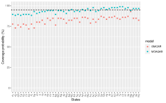
(a) Low

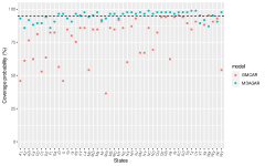
(b) Medium

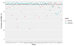
(c) High

Figure S.4: Coverage probability ($\%$) of $corr(w_{1j},w_{2j})$, i.e. correlation between two diseases in each state, for MDAGAR (blue) and GMCAR (red).

Table S.3: Coverage probability ($\%$) of parameters estimated from MDAGAR and GMCAR

		Coverage probability ($\%$)
Correlation	Model	$\eta_{021}$	$\eta_{121}$	$\rho_{1}$	$\rho_{2}$	$\tau_{1}$	$\tau_{2}$	$\sigma_{1}^{2}$	$\sigma_{2}^{2}$
Low	MDAGAR	92.9	95.3	92.9	97.6	100	98.8	100	100
	GMCAR	92.9	80.0	84.7	95.3	95.3	100	83.5	100
Medium	MDAGAR	94.1	97.6	98.8	96.5	98.8	98.8	100	100
	GMCAR	85.9	77.6	69.4	98.8	61.2	98.8	84.7	98.8
High	MDAGAR	92.9	94.1	95.3	54.1	96.5	98.8	78.8	100
	GMCAR	96.5	88.2	70.6	100	1.20	100	97.6	100

S.8 Multiple Cancer Analysis from SEER for Case 2: Exclude smoking rates in covariates

Excluding the risk factor adult cigarette smoking rates, we only include county attributes described in 4 as covariates. Among $24$ models, model $M_{16}$ exhibits dominated best performance with a posteior probability of 0.999 and the corresponding conditional structure is $[\mbox{larynx}]\times[\mbox{esophagus}\,|\,\mbox{larynx}]\times[\mbox{colorectal}\,|\,\mbox{larynx},\mbox{esophagus}]\times[\mbox{lung}\,|\,\mbox{larynx},\mbox{esophagus},\mbox{colorectal}]$.

Table S.4 is a summary of the parameter estimates for each cancer. From $M_{16}$, we find that the regression slope for the percentage of blacks and unemployed residents are significantly positive for larynx and lung cancer respectively. The larynx cancer exhibits weaker spatial autocorrelation while the residual spatial autocorrelation for the other three cancers after accounting for preceding cancers are at moderate levels. For spatial precision $\tau_{i}$, larynx random effects still have the smallest variability while the conditional variability for colorectal and lung cancers are slightly larger.

Table S.4: Posterior means (95$\%$ credible intervals)for parameter estimated from $M_{16}$ for Case 2 (excluding somking rates in covariates).

Parameters	Larynx	Esophageal	Colorectal	Lung
Intercept	6.75 (-0.58, 14.00)	11.14 (-1.70, 24.05)	18.89 (-10.37, 48.12)	24.18 (-22.71, 68.75)
Young($\%$)	-0.09 (-0.20, 0.02)	-0.09 (-0.29, 0.11)	0.27 (-0.19, 0.74)	0.04 (-0.75, 0.86)
Old($\%$)	-0.04 (-0.12, 0.04)	0.00 (-0.15, 0.16)	0.13 (-0.23, 0.49)	0.15 (-0.49, 0.91)
Edu($\%$)	-0.02 (-0.08, 0.04)	-0.02 (-0.13, 0.09)	0.12 (-0.13, 0.38)	-0.34 (-0.82, 0.15)
Unemp($\%$)	0.04 (-0.03, 0.12)	0.06 (-0.08, 0.20)	0.10 (-0.26, 0.45)	1.21 (0.55, 1.89)
Black($\%$)	0.15 (0.03, 0.27)	0.10 (-0.12, 0.32)	-0.20 (-0.75, 0.33)	0.06 (-1.03, 1.13)
Male($\%$)	-0.01 (-0.08, 0.07)	-0.07 (-0.21, 0.06)	0.18 (-0.16, 0.52)	0.01 (-0.59, 0.60)
Uninsured($\%$)	-0.07 (-0.19, 0.04)	-0.13 (-0.33, 0.07)	0.10 (-0.37, 0.58)	0.11 (-0.70, 0.95)
Poverty($\%$)	0.21 (-0.11, 0.53)	0.40 (-0.20, 1.02)	0.03 (-1.38, 1.45)	0.84 (-2.14, 3.52)
$\rho_{i}$	0.25 (0.01, 0.91)	0.49 (0.02, 0.97)	0.43 (0.02, 0.94)	0.50 (0.03, 0.98)
$\tau_{i}$	44.04 (15.89, 90.23)	24.55 (5.06, 61.33)	18.25 (1.39, 51.15)	19.68 (2.00, 55.07)
$\sigma_{i}^{2}$	0.56 (0.37, 0.84)	1.52 (0.88, 2.36)	9.85 (6.48, 14.63)	0.93 (0.18, 3.63)

S.9 Supplementary Figures and Tables

Supplementary figures and tables referenced in Section 3.2, 4 and 5 are shown below.

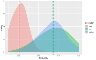
Figure S.5: Density plots for probability that the KL-divergence between the MDAGAR and the true model is smaller than that between GMCAR and the true model with three levels of correlation for two diseases: low (purple), medium (green) and high (red)

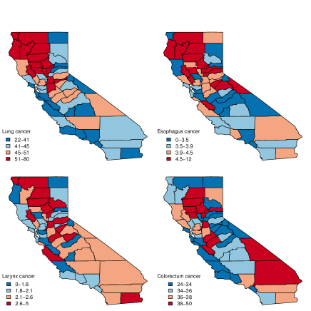
(a) 5-year average age-adjusted incidence rates per 100,000 population for lung, esophagus, larynx and colorectal cancer, 2012 - 2016

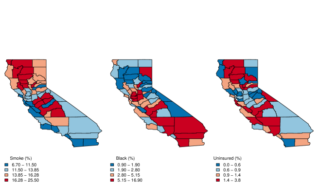
(b) adult cigarette smoking rates (left), percentage of black residents (middle) and uninsured residents (right)

Figure S.6: Maps of county-level raw data in California including (a) incidence rates for lung, esophagus, larynx and colorectal cancer and (b) important county-level covariates with significant effects: adult cigarette smoking rates, percentage of blacks and uninsured residents.

Figure S.7: Posterior distributions of $\bm{\eta}$ for all pairs of cancers.

Figure S.8: Estimated correlation between the incidence of pairwise cancers in each of 58 counties of California for Case 1 vs. Case 2: (a) case 1: esophageal and colorectal cancer, (b) case 1: esophageal and lung cancer, (c) case 1: colorectal and lung cancer, (d) case 2: esophageal and colorectal cancer, (e) case 2: esophageal and lung cancer, (f) case 2: colorectal and lung cancer. Maps (a)-(c) exihibit estimated correlations for Case 1, and (d) - (f) are for Case 2. Yelllow points indicate significant correlations. Note: Maps for larynx cancer are not shown due to non-significant correlation with any of the other three cancers

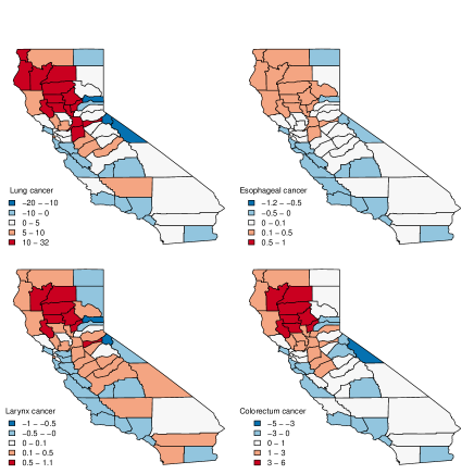
Figure S.9: Maps of posterior mean spatial random effects (with no covariates) using the same order as $M_{10}$

Table S.5: The prosterior model probabilities for 24 models

$p(M_{1}\,|\,\bm{y})$	$p(M_{2}\,|\,\bm{y})$	$p(M_{3}\,|\,\bm{y})$	$p(M_{4}\,|\,\bm{y})$	$p(M_{5}\,|\,\bm{y})$	$p(M_{6}\,|\,\bm{y})$	$p(M_{7}\,|\,\bm{y})$	$p(M_{8}\,|\,\bm{y})$
0.000	0.000	0.000	0.000	0.000	0.000	0.000	0.000
$p(M_{9}\,|\,\bm{y})$	$p(M_{10}\,|\,\bm{y})$	$p(M_{11}\,|\,\bm{y})$	$p(M_{12}\,|\,\bm{y})$	$p(M_{13}\,|\,\bm{y})$	$p(M_{14}\,|\,\bm{y})$	$p(M_{15}\,|\,\bm{y})$	$p(M_{16}\,|\,\bm{y})$
0.000	0.577	0.000	0.000	0.000	0.000	0.342	0.079
$p(M_{17}\,|\,\bm{y})$	$p(M_{18}\,|\,\bm{y})$	$p(M_{19}\,|\,\bm{y})$	$p(M_{20}\,|\,\bm{y})$	$p(M_{21}\,|\,\bm{y})$	$p(M_{22}\,|\,\bm{y})$	$p(M_{23}\,|\,\bm{y})$	$p(M_{24}\,|\,\bm{y})$
0.000	0.000	0.000	0.000	0.000	0.000	0.000	0.002

References

- Banerjee (2020) Banerjee, S. (2020). Modeling massive spatial datasets using a conjugate bayesian linear modeling framework. Spatial Statistics 37, 100417.
- Berke (2004) Berke, O. (2004). Exploratory disease mapping: kriging the spatial risk function from regional count data. International Journal of Health Geographics 3, 18.
- Besag (1974) Besag, J. (1974). Spatial interaction and the statistical analysis of lattice systems. Journal of the Royal Statistical Society: Series B (Methodological) 36, 192–225.
- Besag et al. (1991) Besag, J., York, J., and Mollié, A. (1991). Bayesian image restoration, with two applications in spatial statistics. Annals of the institute of statistical mathematics 43, 1–20.
- Bradley et al. (2015) Bradley, J. R., Holan, S. H., and Wikle, C. K. (2015). Multivariate spatio-temporal models for high-dimensional areal data with application to longitudinal employer-household dynamics. Ann. Appl. Stat. 9, 1761–1791.
- California Department of Public Health (2018) California Department of Public Health (2018). California tobacco control program. california tobacco facts and figures.
- Carlin et al. (2003) Carlin, B. P., Banerjee, S., et al. (2003). Hierarchical multivariate car models for spatio-temporally correlated survival data. Bayesian statistics 7, 45–63.
- Cover and Thomas (1991) Cover, T. M. and Thomas, J. A. (1991). Elements of information theory. Wiley Series in Telecommunications and Signal Processing. Wiley Interscience.
- Daniels et al. (2006) Daniels, M. J., Zhou, Z., and Zou, H. (2006). Conditionally specified space-time models for multivariate processes. Journal of Computational and Graphical Statistics 15, 157–177.
- Datta et al. (2018) Datta, A., Banerjee, S., Hodges, J. S., Gao, L., et al. (2018). Spatial disease mapping using directed acyclic graph auto-regressive (dagar) models. Bayesian Analysis .
- Diva et al. (2008) Diva, U., Dey, D. K., and Banerjee, S. (2008). Parametric models for spatially correlated survival data for individuals with multiple cancers. Statistics in medicine 27, 2127–2144.
- Gamerman and Lopes (2006) Gamerman, D. and Lopes, H. F. (2006). Markov chain Monte Carlo: stochastic simulation for Bayesian inference. Chapman and Hall/CRC.
- Gelfand and Dey (1994) Gelfand, A. E. and Dey, D. K. (1994). Bayesian model choice: asymptotics and exact calculations. Journal of the Royal Statistical Society: Series B (Methodological) 56, 501–514.
- Gelfand and Ghosh (1998) Gelfand, A. E. and Ghosh, S. K. (1998). Model choice: a minimum posterior predictive loss approach. Biometrika 85, 1–11.
- Gelfand and Vounatsou (2003) Gelfand, A. E. and Vounatsou, P. (2003). Proper multivariate conditional autoregressive models for spatial data analysis. Biostatistics 4, 11–15.
- Gelman et al. (2014) Gelman, A., Hwang, J., and Vehtari, A. (2014). Understanding predictive information criteria for bayesian models. Statistics and computing 24, 997–1016.
- Gronau et al. (2017) Gronau, Q. F., Sarafoglou, A., Matzke, D., Ly, A., Boehm, U., Marsman, M., Leslie, D. S., Forster, J. J., Wagenmakers, E.-J., and Steingroever, H. (2017). A tutorial on bridge sampling. Journal of mathematical psychology 81, 80–97.
- Gronau et al. (2017) Gronau, Q. F., Singmann, H., and Wagenmakers, E.-J. (2017). Bridgesampling: An r package for estimating normalizing constants. arXiv preprint arXiv:1710.08162 .
- Held et al. (2005) Held, L., Natário, I., Fenton, S. E., Rue, H., and Becker, N. (2005). Towards joint disease mapping. Statistical methods in medical research 14, 61–82.
- Hoeting et al. (1999) Hoeting, J. A., Madigan, D., Raftery, A. E., and Volinsky, C. T. (1999). Bayesian model averaging: a tutorial. Statistical science pages 382–401.
- Jin et al. (2007) Jin, X., Banerjee, S., and Carlin, B. P. (2007). Order-free co-regionalized areal data models with application to multiple-disease mapping. Journal of the Royal Statistical Society: Series B (Statistical Methodology) 69, 817–838.
- Jin et al. (2005) Jin, X., Carlin, B. P., and Banerjee, S. (2005). Generalized hierarchical multivariate car models for areal data. Biometrics 61, 950–961.
- Kim et al. (2001) Kim, H., Sun, D., and Tsutakawa, R. K. (2001). A bivariate bayes method for improving the estimates of mortality rates with a twofold conditional autoregressive model. Journal of the American Statistical association 96, 1506–1521.
- Kissling and Carl (2008) Kissling, W. D. and Carl, G. (2008). Spatial autocorrelation and the selection of simultaneous autoregressive models. Global Ecology and Biogeography 17, 59–71.
- Knorr-Held and Best (2001) Knorr-Held, L. and Best, N. G. (2001). A shared component model for detecting joint and selective clustering of two diseases. Journal of the Royal Statistical Society: Series A (Statistics in Society) 164, 73–85.
- Koch (2005) Koch, T. (2005). Cartographies of disease: maps, mapping, and medicine. Esri Press Redlands, CA.
- Lindström et al. (2017) Lindström, S., Finucane, H., Bulik-Sullivan, B., Schumacher, F. R., Amos, C. I., Hung, R. J., Rand, K., Gruber, S. B., Conti, D., Permuth, J. B., et al. (2017). Quantifying the genetic correlation between multiple cancer types. Cancer Epidemiology and Prevention Biomarkers 26, 1427–1435.
- Marí-Dell’Olmo et al. (2014) Marí-Dell’Olmo, M., Martinez-Beneito, M. A., Gotsens, M., and Palència, L. (2014). A smoothed anova model for multivariate ecological regression. Stochastic environmental research and risk assessment 28, 695–706.
- Martinez-Beneito (2013) Martinez-Beneito, M. A. (2013). A general modelling framework for multivariate disease mapping. Biometrika 100, 539–553.
- Meng and Wong (1996) Meng, X.-L. and Wong, W. H. (1996). Simulating ratios of normalizing constants via a simple identity: a theoretical exploration. Statistica Sinica pages 831–860.
- National Cancer Institute (2019) National Cancer Institute (2019). Seer*stat software.
- Perrakis et al. (2014) Perrakis, K., Ntzoufras, I., and Tsionas, E. G. (2014). On the use of marginal posteriors in marginal likelihood estimation via importance sampling. Computational Statistics & Data Analysis 77, 54–69.
- Richardson et al. (2004) Richardson, S., Thomson, A., Best, N., and Elliott, P. (2004). Interpreting posterior relative risk estimates in disease-mapping studies. Environmental health perspectives 112, 1016–1025.
- Robert and Casella (2004) Robert, C. and Casella, G. (2004). Monte carlo statistical methods springer-verlag. New York .
- Rua and Held (2005) Rua, H. and Held, L. (2005). Gaussian Markov Random Fields : Theory and Applications. Monographs on statistics and applied probability. Chapman and Hall/CRC Press, Boca Raton, FL.
- Watanabe (2010) Watanabe, S. (2010). Asymptotic equivalence of bayes cross validation and widely applicable information criterion in singular learning theory. Journal of Machine Learning Research 11, 3571–3594.
- Zhang et al. (2009) Zhang, Y., Hodges, J. S., and Banerjee, S. (2009). Smoothed anova with spatial effects as a competitor to mcar in multivariate spatial smoothing. The annals of applied statistics 3, 1805.
- Zhu et al. (2005) Zhu, J., Eickhoff, J. C., and Yan, P. (2005). Generalized linear latent variable models for repeated measures of spatially correlated multivariate data. Biometrics 61, 674–683.