Percolation theory of self-exciting temporal processes

Abstract

We investigate how the properties of inhomogeneous patterns of activity, appearing in many natural and social phenomena, depend on the temporal resolution used to define individual bursts of activity. To this end, we consider time series of microscopic events produced by a self-exciting Hawkes process, and leverage a percolation framework to study the formation of macroscopic bursts of activity as a function of the resolution parameter. We find that the very same process may result in different distributions of avalanche size and duration, which are understood in terms of the competition between the 1D percolation and the branching process universality class. Pure regimes for the individual classes are observed at specific values of the resolution parameter corresponding to the critical points of the percolation diagram. A regime of crossover characterized by a mixture of the two universal behaviors is observed in a wide region of the diagram. The hybrid scaling appears to be a likely outcome for an analysis of the time series based on a reasonably chosen, but not precisely adjusted, value of the resolution parameter.

Inhomogeneous patterns of activity, characterized by bursts of events separated by periods of quiescence, are ubiquitous in nature Karsai et al. (2018). The firing of neurons Dalla Porta and Copelli (2019); Beggs and Plenz (2003), earthquakes Bak et al. (2002), energy release in astrophysical systems Wang and Dai (2013) and spreading of information in social systems Barabasi (2005); Karsai et al. (2012); Gleeson et al. (2014) exhibit bursty activity, with intensity and duration of bursts obeying power-law distributions Dalla Porta and Copelli (2019); Beggs and Plenz (2003); Karsai et al. (2012).

If activity consists of point-like events in time, size and duration of bursts are obtained from the inter-event time sequence. The analysis of many systems Fontenele et al. (2019); Barabasi (2005); Karsai et al. (2012); Weng et al. (2012); Bak et al. (2002) reveals that the inter-event time between consecutive events has a fat-tailed distribution Barabasi (2005); Bak et al. (2002); Karsai et al. (2012). This distribution appears more reliable for the characterization of correlation in bursty systems than other traditional measures, e.g., the autocorrelation function Karsai et al. (2012); Jo et al. (2015); Kumar et al. (2020). However, the relation between autocorrelation and burst size distribution is opaque. Further complications arise as the separation between different bursts is not clear-cut. In discrete time series, avalanches of correlated activity are monitored by coarsening the time series at a fixed temporal scale, and correlations are measured by assigning events to the same burst if their inter-event time is smaller than a given threshold  Karsai et al. (2012). The threshold is set equal to some arbitrarily chosen value and/or imposed by the temporal resolution at which empirical data are acquired, despite its potential of affecting the properties of the resulting distributions Pasquale et al. (2008); Neto et al. (2019); Miller et al. (2019); Chiappalone et al. (2005); Levina and Priesemann (2017); Janićević et al. (2016); Villegas et al. (2019).

The purpose of the present letter is to understand the relation between temporal resolution and burst statistics. We introduce a principled technique to determine the value of the time resolution that should be used to define avalanches from time series. We validate the method on time series generated according to an Hawkes process Hawkes (1971), a model of autocorrelated behavior used for the description of earthquakes Helmstetter and Sornette (2002); Ogata (1988), neuronal networks Kossio et al. (2018), and socio-economic systems Crane and Sornette (2008); Sornette et al. (2004). The use of the Hawkes process affords us a complete control over the mechanism that generates correlations and the possibility to attack the problem analytically.

We start by defining a cluster of activity consistently with the informal notion of a burst composed of close-by events. Data are represented by $K$ total events $\{t_{1},\ldots,t_{K}\}$, where $t_{i}$ is the time of appearance of the $i$-th event. We fix a resolution parameter $\Delta\geq 0$ to identify clusters of activity. A cluster starting at time $t_{b}$ is given by the $S$ consecutive events $\{t_{b},t_{b+1},\ldots,t_{b+S-1}\}$ such that $t_{b}-t_{b-1}>\Delta$, $t_{b+S}-t_{b+S-1}>\Delta$, and $t_{b+i}-t_{b+i-1}\leq\Delta$ for all $i=1,\ldots,S$. We assume $t_{0}=-\infty$ and $t_{K+1}=+\infty$, implying that the first and the last events open and close a cluster, respectively. We define the size $S$ as the number of events within the cluster, and its duration as $T=t_{b+S-1}-t_{b}$, i.e., the time lag between the first and last event in the cluster.

If $\Delta$ is larger than the largest inter-event time, then we have a single cluster of size $K$ and duration $t_{K}-t_{1}$. On the other hand, if $\Delta$ is smaller than the smallest inter-event time, each event is a cluster of size 1 and duration 0. As in 1D percolation problems Stauffer and Aharony (1994), we expect for an intermediate value $\Delta=\Delta^{*}$ a transition from the non-percolating to the percolating phase. What can we learn from the percolation diagram of the time series? Does fixing $\Delta=\Delta^{*}$ allow us to observe properties of the process otherwise not apparent?

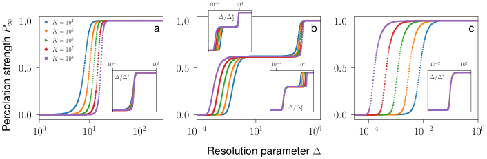
Figure 1: Percolation phase diagrams of self-exciting temporal processes. We plot the percolation strength $P_{\infty}$ as a function of the resolution parameter $\Delta$ for various configurations of the rate of Eq. (1), with exponential kernel function and various system sizes $K$. Average values are obtained by considering $R=10^{3}$ realizations of the process. (a) We set $n=0$ and $\mu=1$. The inset shows the same data as of the main with abscissa rescaled as $\Delta/\Delta^{*}$. (b) We set $n=1$ and $\mu=10^{-4}$. The insets display the same data as of the main, but with rescaled abscissa, $\Delta/\Delta_{1}^{*}$ in the lower inset, and $\Delta/\Delta_{2}^{*}$in the upper inset. (c) We set $n=1$ and $\mu=10^{2}$. The inset shows the same data as of the main, but with abscissa rescaled as $\Delta/\Delta^{*}$.

We address the above questions in a controlled setting where we generate time series via an Hawkes process Hawkes (1971); Hawkes and Oakes (1974) with conditional rate

$$\lambda(t|t_{1},\ldots,t_{k})=\mu+n\,\sum_{i=1}^{k}\,\phi(t-t_{i})\;.$$ (1)

The rate depends on the $k$ earlier events happened at times $t_{1}\leq t_{2}\leq\ldots\leq t_{k}\leq t$. The first term in Eq. (1) produces spontaneous events at rate $\mu\geq 0$. The second term consists of the sum of individual contributions from each earlier event, with the $i$-th event happened at time $t_{i}\leq t$ increasing the rate by $\phi(t-t_{i})$. $\phi(x)$ is the excitation or kernel function of the self-exciting process, and it is assumed to be non-negative and monotonically non-increasing. Typical choices for the kernel are exponential or power-law decaying functions. We will consider both cases. In Eq. (1), we assume $\int_{0}^{\infty}\,\phi(x)\,dx=1$, so that the memory term is weighted by the single parameter $n\geq 0$. Unless otherwise stated, we always set $n=1$, corresponding to the critical dynamical regime of the temporal point process described by Eq. (1) Helmstetter and Sornette (2002).

The percolation framework allows us to characterize the generic Hawkes process of Eq. (1) using finite-size scaling analysis Stauffer and Aharony (1994) (SM, sec. C). The total number $K$ of events in the time series is the system size. For a given value of $K$, we generate multiple time series and compute the percolation strength $P_{\infty}$, i.e., the fraction of events belonging to the largest cluster, and the associated susceptibility (SM, sec. C). By studying the behavior of these macroscopic observables as $K$ grows, we estimate the values of the thresholds and the critical exponents.

Let us start with the case $n=0$ (Figure 1a), describing a homogeneous Poisson process with rate $\mu$. The generic inter-event time $x_{i}=t_{i}-t_{i-1}$ is a random variate distributed as $P(x_{i})=\mu\,e^{-\mu\,x_{i}}$. Two consecutive events are part of the same cluster with probability $P(x_{i}\leq\Delta)=1-e^{-\mu\Delta}$, which is independent of the index $i$ and represents an effective bond occupation probability in a homogeneous 1D percolation model Stauffer and Jayaprakash (1978); Stauffer and Aharony (1994). For finite $K$ values, $P_{\infty}$ sharply grows from $0$ to $1$ around the pseudo-critical point $\Delta^{*}(K)=\log(K)/\mu$ (SM, sec. D). Finite-size scaling analysis indicates that the transition is discontinuous, as expected for 1D ordinary percolation Stauffer and Aharony (1994). We note that the distributions of cluster size $P(S)$ and duration $P(T)$ are exactly described by the 1D percolation theory Stauffer and Aharony (1994) (SM, sec. D). They are the product of a power-law function and a fast-decaying scaling function accounting for the system finite size Stauffer and Jayaprakash (1978). In this specific case, the scaling functions contain a multiplicative term that exactly cancels the power-law term of the distribution. Therefore, the distributions have exponential behavior at $\Delta=\Delta^{*}$. A clear signature of criticality is manifest in the relation between size and duration, $\langle S\rangle\sim T$, in agreement with the relation $\langle S\rangle\sim T^{(\alpha-1)/(\tau-1)}$ (SM, sec. D).

We now consider the Hawkes process of Eq. (1) with exponential kernel $\phi(x)=e^{-x}$ Hawkes and Oakes (1974); Dassios and Zhao (2013). Results of our finite-size scaling analysis are reported in Figures 1b and  1c, for $\mu\ll 1$ and $\mu\gg 1$, respectively.

For $\mu\ll 1$, the phenomenology is rich, with two distinct transitions at $\Delta^{*}_{1}<\Delta^{*}_{2}$, respectively. Around the critical point $\Delta_{1}^{*}$, the system is characterized by a behavior compatible with the universality class of 1D percolation, i.e, the same as of the homogeneous Poisson process. Both $P(S)$ and $P(T)$ display power-law decays at $\Delta_{1}^{*}$, with exponent values $\tau=\alpha=2$ (Figures 2a and 2c). Average size and duration of clusters are linearly correlated (SM, sec. E). The pseudo-critical threshold equals $\Delta^{*}_{1}(K)\simeq\log(K)/\langle{\lambda}\rangle=\log(K)/\left(\mu+\sqrt{2K\mu}\right)$, thus leading to a vanishing critical point in the thermodynamic limit (SM, sec. E). $\langle{\lambda}\rangle$ is the expectation value, over an infinite number of realizations of the process, of the rate after $K$ events have happened; the estimate of the critical point $\Delta^{*}_{1}(K)$ is thus obtained using the same exact equation as for a homogeneous Poisson process with effective rate $\langle{\lambda}\rangle$. The other transition at $\Delta^{*}_{2}(K)=\log(K)/\mu$, which tends to infinite as $K$ grows, corresponds to the merger of the whole time series into one cluster; its features are compatible with those of the universality class of the mean-field branching process, i.e., $\tau=3/2$ and $\alpha=2$. The region of the phase diagram $[\Delta^{*}_{1}(K),\Delta^{*}_{2}(K)]$, which is expanding as $K$ increases, is characterized by critical behavior. While the percolation strength plateaus at $P_{\infty}\simeq 1-1/e\simeq 0.63$, the susceptibility is larger than zero. Furthermore, the distribution $P(S)$ displays a neat crossover between the regime $\tau=2$ for small $S$ and the regime $\tau=3/2$ at large $S$ (Figure 2a).

For $\mu\gg 1$, the phase diagram displays a single transition (Figure 1c), with features identical to those described for the case $\mu\ll 1$ around $\Delta_{1}^{*}$: no crossover is present, and the critical exponents of the distributions $P(S)$ and $P(T)$ are $\tau=\alpha=2$ (Figures 2b and  2d). The same exact behavior can be obtained by simply considering a non-homogeneous Poisson process with rate linearly growing in time, i.e., $\lambda(t)\sim t$ (SM, Sec. K).

The two different behaviors observed for $\mu\ll 1$ and $\mu\gg 1$ are interpreted in an unified framework as follows. For $\mu\ll 1$, the process is characterized by a sequence of self-exciting bursts due to the memory term of the rate of Eq. (1). Memory decays exponentially fast, with a typical time scale equal to 1. Each burst is started by a spontaneous event. Since spontaneous events are characterized by the time scale $1/\mu\gg 1$, consecutive bursts are well separated one from the other. Increasing $\Delta$, the system exhibits first a transition ”within bursts” at $\Delta=\Delta_{1}^{*}$, corresponding to the merger of events within the same burst, and then a transition ”across bursts” at $\Delta=\Delta_{2}^{*}$, corresponding to the merger of consecutive bursts of activity. For $\mu\gg 1$, all events belong to a unique burst of self-excitation. The time scale of spontaneous activity is equal or smaller than the one due to self-excitation. Thus, although the memory decays exponentially fast, a new spontaneous event re-excites the process quickly enough to allow the burst to proceed its activity uninterrupted. The burst is truncated in the simulations due to the fixed size $K$ of the time series. As $\Delta$ increases, all events of the single burst are merged into a single cluster. The transition is therefore of the same type as the one observed within bursts at $\Delta=\Delta_{1}^{*}$ in the case $\mu\ll 1$.

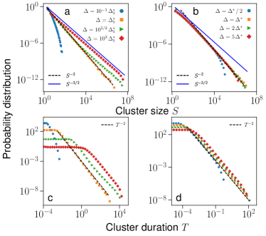
Figure 2: Critical properties of self-exciting temporal processes. We consider processes generated from the rate of Eq. (1) with exponential kernel and $n=1$. System size $K=10^{8}$. Histograms obtained by considering $C=10^{7}$ clusters per configuration. (a) Cluster size distribution for $\mu=10^{-4}$. (b) Cluster size distribution for $\mu=10^{2}$. (c) Cluster duration distribution for the same data as in panel a. (d) Cluster duration distribution for the same data as in panel b.

We can separately study the transitions within and across bursts. To this end, we simplify the actual process of Eq. (1) by setting $\mu=0$ and assuming that the first event of the burst already happened. We then invoke the known mapping of the self-exciting process of Eq. (1) to a standard Galton-Walton branching process (BP) Hawkes and Oakes (1974). According to it, the first event of the time series represents the root of a branching tree (Figure 3). Each event generates a number of follow-up events (offsprings) obeying a Poisson distribution with expected value equal to $n$, the parameter appearing in Eq. (1). Time is assigned as follows. The first event happens at an arbitrary time $t_{1}$, say for simplicity $t_{1}=0$. Then each of the following events has associated a time equal to the time of its parent plus a random variate $x$ extracted from the kernel function $\phi(x)$ of Eq. (1). The mapping to the BP offers an alternative (on average statistically equivalent) way of generating time series for the self-exciting process of Eq. (1). We first generate a BP tree, and then associate a time to each event of the tree according to the rule described above. The time $t$ associated to a generic event of the $g$-th generation is distributed according to a function $P(t|g)$. For the exponential kernel function, $P(t|g)$ is the sum of $g$ exponentially distributed variables, i.e., the Erlang distribution with rate equal to 1, $P(t|g)=t^{g-1}\,e^{-t}/(g-1)!$.

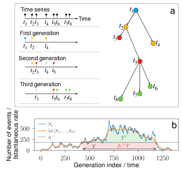
Figure 3: Latent tree structure of self-exciting temporal processes. (a) Each event in the time series on the left is associated to a parent node. On the right, the branching tree corresponding to the time series. Each node is assigned to a generation, and each bond has associated an inter-event time. If $N_{g}$ is the number of nodes in the $g$-th generation, the depicted tree has $\{N_{1}=1,N_{2}=2,N_{3}=2,N_{4}=3,\ldots\}$. (b) The mapping of panel a allows us to associate to the tree $\{N_{1},\dots,N_{G}\}$ (blue curve) an inhomogeneous Poisson process with instantaneous rate $\tilde{\lambda}(t|N_{1},\ldots,N_{G})$ (orange). Such a process generates time series statistically equivalent to those generated by an Hawkes process with latent tree structure $\{N_{1},\ldots,N_{G}\}$. The inverse resolution parameter $\Delta^{-1}$ (dashed black line) is an effective threshold for the Poisson process $\tilde{\lambda}(t|N_{1},\ldots,N_{G})$. As a result, size and duration of clusters are related by Eq. (2). The shaded areas denote the two terms appearing on the rhs of Eq. (2).

The mapping of the self-exciting process to a BP allows us to fully understand the numerical findings of Figures 1 and 2. For $n=1$ the BP is critical. The distribution of the tree size is $P(Z)\sim Z^{-3/2}$ and the distribution of the tree depth is $P(D)\sim D^{-2}$. Individual bursts of activity, as seen for sufficiently high $\Delta$ values and $\mu\ll 1$, obey this statistics. Specifically, the size of each burst $S$ is exactly the size $Z$ of the tree. The average duration of the bursts $\langle T\rangle\sim D$, as expected for the sum of iid exponentially distributed random variates. For $\Delta\in[\Delta_{1}^{*},\Delta_{2}^{*}]$, $P_{\infty}$ of Figure 1b follows the same statistics as the maximum value of a sample of variables extracted from the distribution $P(Z)\sim Z^{-3/2}$ divided by their sum, and the average value of the ratio plateaus at $1-1/e$ for sufficiently large sample sizes, fully explaining the results of Figure 1 (SM, sec. H).

The behavior at $\Delta=\Delta_{1}^{*}$ and the crossover towards the standard BP regime for larger $\Delta$ are due to a threshold phenomenon. This directly follows from the abrupt nature of the percolation transition of the Poisson process (Figure 1a). Given the latent branching tree $\{N_{1},N_{2},\ldots,N_{g},\ldots,N_{G}\}$, where $N_{g}$ indicates the number of events of the $g$-th generation of the tree, the time series of the Hawkes process is statistically equivalent to the one of the inhomogeneous Poisson process with instantaneous rate $\tilde{\lambda}(t|N_{1},\ldots,N_{G})=\sum_{g}\,P(t|g)\,N_{g}$. Hence, for a given $\Delta$, as long as $\tilde{\lambda}(t|N_{1},\ldots,N_{G})>1/\Delta$, all events are part of the same cluster of activity; when instead $\tilde{\lambda}(t|N_{1},\ldots,N_{G})<1/\Delta$, then events around time $t$ belong to separate clusters of activity. As a consequence, the total number of events $S_{T}$ that form a cluster of activity of duration $T$ is the integral of the curve $\tilde{\lambda}(t|N_{1},\ldots,N_{G})$ in the time interval when the rate is above $\Delta^{-1}$ (Figure 3b). We repeat a similar calculation as in Ref. Villegas et al. (2019). The integral can be split in two contributions, one corresponding to the area of the order of $T^{2}$ appearing above the threshold line, as expected for a critical BP di Santo et al. (2017); Villegas et al. (2019), and the other corresponding to the area $\Delta^{-1}\,T$ appearing below threshold,

$$S_{T}\sim T^{2}+\Delta^{-1}\,T\;.$$ (2)

While the distribution of cluster durations is always the same [i.e., $P(T)\sim T^{-2}$ of the underlying BP], if $\Delta^{-1}>T$ then $S_{T}\sim T$ implying the within-burst statistics $P(S)\sim S^{-2}$. Instead, if $\Delta^{-1}<T$ then $S_{T}\sim T^{2}$ and the conservation of probability leads to the BP statistics $P(S)\sim S^{-3/2}$. When the two terms on the rhs of Eq. (2) have comparable magnitude, a crossover between the two scalings occurs. The crossover point varies with the temporal resolution as $S_{c}\propto\Delta^{-2}$ (SM, sec. G). A full understanding of $P(S)$ is achieved by noting that power-law scaling requires a minimum sample size to be observed, sufficient for the largest cluster to have duration comparable to $1/\Delta_{1}^{*}$. If the sample is not large enough the distribution will appear as exponential (SM, sec. G).

We finally consider the power-law kernel function $\phi(x)=(\gamma-1)(1+x)^{-\gamma}$. The branching structure underlying the process is not affected by the kernel so the results above should continue to hold Helmstetter and Sornette (2002). For $\gamma>2$, $\phi(x)$ has finite mean value and, as a consequence, results are identical to those obtained for the exponential kernel (SM, Sec. G). Specifically, $P_{\infty}$ shows a discontinuous transition when $\mu\gg 1$, while two sharp transitions are observed for $\mu\ll 1$. The distribution of cluster sizes exhibits a crossover from $\tau=2$ at $\Delta^{*}_{1}$ to $\tau=3/2$ for $\Delta\gg\Delta_{1}^{*}$ when $\mu\ll 1$, and the exponent $\tau=2$ with no crossover when $\mu\gg 1$. If $\gamma\leq 2$, $\phi(x)$ has diverging mean value, the typical inter-event time is large preventing the present framework to be applicable.

In summary, we investigated how self-excitation mechanisms are reflected in the bursty dynamics, exploring their relationship with avalanche distributions, which offer an effective probe into the presence of autocorrelation in time series Karsai et al. (2018). We focused on the Hawkes process, a general mechanism to produce self-excitation, autocorrelation, and fat-tailed distributions in the avalanche size and duration. Critical behavior in the distributions is observed at specific values of the resolution parameter $\Delta$, and is characterized by exponents independent of the form of the self-excitation mechanism. The universal critical behavior is governed by both the branching structure underlying the Hawkes process and the features of 1D percolation. Nontrivial details of the size distribution depend on the relative force of the spontaneous and self-excitation mechanisms. The two classes of behavior coexist for a wide range of $\Delta$ values, thus making the observation of a mixture of two classes the most likely outcome of an analysis where the resolution parameter is not fine-tuned. All findings extend to the slightly subcritical configuration of the Hawkes process (SM, Sec. I), thus showing that our method is scientifically sound also for the analysis of avalanches in some natural systems possibly operating close to, but not exactly in, a critical regime Priesemann et al. (2014). Our work offers an interpretative framework for the relationship between avalanche properties and the mechanisms producing autocorrelation in bursty dynamics. More work in this area is nevertheless needed. The Hawkes process is unable to reproduce the variety of critical behaviors reported for real data sets in Ref. Karsai et al. (2018), and other self-excitation mechanisms need to be considered.

Supplemental Material

.1 Hawkes process: numerical simulations

.1.1 Exponential kernel

The Markov property of the exponential kernel can be exploited to numerically simulate the process in linear time by means of the algorithm developed in Ref. Dassios and Zhao (2013). In the present case of unmarked Hawkes process the implementation is straightforward. Given the rate $\lambda(t_{k-1})$ right after the $(k-1)$-th event, the $k$-th inter-event time can be sampled as

1. Set $F_{1}=-\log(u_{1})/\mu,\text{ where }u_{1}\sim\text{Unif}(0,1)$.

2. Set $G_{2}=1+\log(u_{2})/(\lambda(t_{k-1})-\mu),\text{ where }u_{2}\sim\text{Unif}(0,1)$.

3. Set $F_{2}=\begin{cases}\infty\,\text{ \quad\quad\quad if }G_{2}\leq 0\\ -\log(G_{2})\text{ \, if }G_{2}>0\end{cases}$ .

4. Set $x_{k}=\text{min}\{F_{1},F_{2}\}$.

5. Set $\lambda(t_{k-1}+x_{k})=(\lambda(t_{k-1})-\mu)e^{-x_{k}}+n+\mu$.

.1.2 Power-law kernel

To generate time series from an Hawkes process with power-law kernel we take advantage of the thinning algorithm by Ogata Ogata (1981). The computational complexity of the algorithm grows quadratically with the number of events. The thinning algorithm requires knowledge of the full history $\{t_{1},t_{2},...,t_{k-1}\}$ of the process for the $k$-th inter-event to be sampled. Specifically, given $\lambda(t_{k-1})$ and the set of previous event times,

1. Set $x=-\log(u_{1})/\lambda(t_{k-1}),\text{ where }u_{1}\sim\text{Unif}(0,1)$.

2. Compute $\lambda(t_{k-1}+x)$ and compute the ratio $\ell=\lambda(t_{k-1}+x)/\lambda(t_{k-1})$.

3. Sample $u_{2}\sim\text{Unif}(0,1)$.

4. If $u_{2}\leq\ell$, set $t_{k}=t_{k-1}+x$. Note that $\lambda(t_{k})=\lambda(t_{k-1}+x)+n(\gamma-1)$, where the first term on the right hand side has been computed at step 2.

Note that, for efficiency reasons, time can be updated even if the event is rejected (i.e. $u_{2}>\ell$) and $\lambda(t_{k-1}+x)$ can be used in step 1 instead of $\lambda(t_{k-1})$ Rizoiu et al. (2017).

.1.3 Leveraging the equivalence with the branching process to generating time series for the Hawkes process

As stated in the main text, a statistically equivalent way to produce time series with the rate of Eq. (1) is to generate a branching tree with the Poisson offspring distribution $P(o;n)$ and then to assign an event time to each node. The inter-event time $x$ between successive generation’s nodes is a random variable with distribution $\phi(x)$. This type of simulations is particularly useful to explore the large-scale properties of the process with the power-law kernel, in that the quadratic scaling of the thinning algorithm with $K$ prevents large time series to be generated.

.2 Critical Hawkes process: average rate

Theorem 3.6 and Corollary 3.5 in Ref. Dassios and Zhao (2011) can be reformulated for the rate of Eq. (1) in the case of exponential kernel. The rate in Ref. Dassios and Zhao (2011) takes the form of Eq. (1) by simply setting, in Ref. Dassios and Zhao (2011) notation, $a=\lambda_{0}=\mu$, $\delta=1$, $Y_{i}=0$ and $Z_{i}=n$ for all $i$. Then Theorem 3.6 and Corollary 3.5 take the form

$$\begin{split}&\langle{\lambda(t)}\rangle=\mu(1+t)\\ &\langle{\lambda^{2}(t)}\rangle=\mu^{2}+(2\mu+n^{2})(\mu t+\mu t^{2}/2)\end{split}\,$$ (S3)

respectively for $n=1$. In Eq. (S3), $\langle\cdot\rangle$ indicates average value over an infinite number of realizations of the Hawkes process. It follows that

$$\frac{\langle{\lambda^{2}(t)}\rangle-\langle{\lambda(t)}\rangle^{2}}{\langle{\lambda(t)}\rangle^{2}}=\frac{1}{2\mu}$$ (S4)

for large time. Thus the process experiences fluctuations that are much smaller than the average rate for $\mu\gg 1$ and vice versa. By noting that the number of events at time $t$, namely $k(t)$, obeys $dk(t)/dt=\lambda(t)$, it is easy to see that $\langle{k(t)}\rangle=\mu\left(t+t^{2}/2\right)$. It follows that for $t\ll 1$ the Hawkes process behaves as a Poisson process, being $\langle{\lambda}\rangle\approx\mu$ and $\langle{k}\rangle(t)\approx\mu t$, while for large time we have that $\langle{\lambda}\rangle\approx\mu t$ and $\langle{k}\rangle(t)\approx\mu t^{2}/2$. Finally, inverting the relation between time and number of events, the average rate is

$$\langle{\lambda(k)}\rangle=\mu+\sqrt{2\mu k}\,.$$ (S5)

The equations above allow to understand the physical interpretation of the phase diagram of Figure 1 of the main paper. In Figure S4a, the average rate is shown and compared to individual realizations of the process. For $\mu\ll 1$, the individual realization is characterized by a sequence of bursts during which the rate grows proportionally to the square root of the event number, in agreement with Eq. (S5). A burst ends when a fluctuation of the rate is large enough for it to drop much below its average value. Strong fluctuations correspond to inter-event times much larger than $1$. They are expected to occur as predicted by Eq. (S4). Large inter-event times make all the individual terms in the kernel small, with the rate dropping to its minimal value, i.e., $\lambda=\mu$. Then, a new event occurring after an inter-event time of the order of $\mu^{-1}$ gives rise to a new burst of the self-exciting process. When instead $\mu\gg 1$, fluctuations are expected to be smaller than the average value. The temporal scales of the spontaneous activity and of the self-exciting process are comparable, so that spontaneously generated events reinforce the burst instead of interrupting it.

The quadratic scaling $\langle{k(t)}\rangle\approx\mu t^{2}/2$ observed at large times is the signature of the branching process underlying the evolution of $\lambda$. The number of events grows as the square of time, in the same way as the size of a branching process grows as the square of the number of generations. This fact can also be seen by noting that $\lambda\sim\sqrt{k}$ and that the typical inter-event time is of the order of $1/\lambda$. We are not aware of explicit formulas for the average rate in the case of the power-law kernel. However, it is not surprising to see, in numerical simulations, $\lambda$ growing with the square root of $k$ for this kernel as well (Figure S4b).

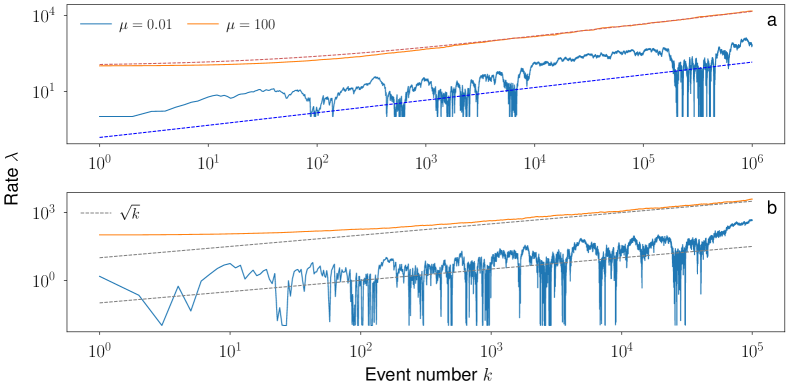
Figure S4: Individual realizations of the critical Hawkes process. (a) Exponential kernel. Two realizations of the process, one for $\mu=0.01$ and one for $\mu=100$. Each realization is compared with the average rate in Eq. S3, shown as a dashed line. (b) Same as before but using a power law kernel with $\gamma=2.5$. The dashed line here simply scales as $\sqrt{k}$.

.3 Finite-size scaling analysis

The percolation strength is defined as the average size of the largest cluster, $S_{M}$, normalized to $K$:

$$P_{\infty}=\frac{\langle{S_{M}}\rangle}{K}\,.$$ (S6)

The susceptibility associated to the order parameter can be defined as

$$\chi=\frac{\langle{S_{M}^{2}}\rangle-\langle{S_{M}}\rangle^{2}}{\langle{S_{M}}\rangle}\,.$$ (S7)

Averages are meant over an infinite number of realizations of the Hawkes process.

The cluster number $n_{S}$ is usually defined as the number of clusters of size $S$ per unit lattice site Stauffer and Aharony (1994). The same definition can be used for the cluster duration $n_{T}$. In percolation theory, the scaling ansatz for the cluster number is formulated as

$$\begin{split}&n_{S}=S^{-\tau}\mathscr{G}_{S}(z)\\ &z=(p_{c}-p)S^{\sigma}\,,\end{split}$$ (S8)

where $p$ is the concentration (i.e., the bond occupation probability) and $p_{c}$ is the critical point of the model. Homogeneous percolation in one dimension has $p_{c}=1$. The scaling ansatz is assumed to be valid in the vicinity of the critical point and for sizes $S\gg 1$ Stauffer and Aharony (1994). Despite the scaling function is, in principle, unknown, it is expected to decay fast after a crossover whose typical scale is

$$S_{c}\propto|p-p_{c}|^{-1/\sigma}\,.$$ (S9)

Equations (S8, S9) define the exponents $\tau$ and $\sigma$, respectively quantifying the decay of the cluster number and the divergence of the crossover scale. All the other critical exponents can be computed via scaling relations involving $\tau$ and $\sigma$. Cluster duration, on a lattice, is the same observable as the cluster size. On disordered topologies, we assume that a scaling form analogous to Eq. (S8) exists for the cluster duration, with $n_{T}$ characterized by its own exponents $\alpha$ and $\sigma_{T}$ and by its own scaling function $\mathscr{G}_{T}$.

Given the scaling of Eq. (S8), the order parameter is expected to grow from zero to a positive value as a power law with exponent $\beta$. The critical exponent $\beta$ can be determined using the knowledge of $\tau$ and $\sigma$, according to

$$\begin{split}&P_{\infty}\propto(p-p_{c})^{\beta}\text{ for }p\rightarrow p_{c}^{+}\,,\\ &\beta=\frac{\tau-2}{\sigma}\,.\end{split}$$ (S10)

In the vicinity of the critical point the susceptibility (S7) diverges as a power law

$$\begin{split}&\chi\propto|p-p_{c}|^{-(\gamma+\beta)}\\ &\gamma=\frac{3-\tau}{\sigma}\,.\end{split}$$ (S11)

The presence of the exponent $\beta$ in the above expression is direct a consequence of the definition of Eq. (S7) Colomer-de Simón and Boguñá (2014).

Critical exponents can be evaluated by means of Finite-Size Scaling (FSS) analysis. The key concept underlying FSS is the existence of a unique length scale characterizing the behaviour of an infinite system. This is the correlation length $\xi$, which represents the typical linear size of the largest (but finite) cluster. The correlation length is in fact defined as the typical scale of the correlation function, which has the exponential form $g(r)=e^{-r/\xi}$ for $p<p_{c}$. The correlation function, in turn, is defined as the probability that a site at distance $r$ from an active site belongs to the same cluster. The correlation length diverges as $|p-p_{c}|^{-\nu}$ in the vicinity of the critical point, indicating that the largest cluster spans the whole lattice. This divergence, however, is de facto bounded by $K$ in finite systems, with $K$ the linear size of the system. Then in any finite system, at any $p$ value, there are two possibilities: $p$ is close enough to $p_{c}$, so that $\xi\gg K$, or $p$ is far enough from $p_{c}$ and $\xi\ll K$.

A second crucial property is the nature of the critical point: $p_{c}$ is a thermodynamic quantity. Critical behavior in finite systems is observed at a different value of the concentration $p$, namely $p^{*}$. The pseudo (size-dependent) critical point scales with the system size according to

$$p_{c}-p^{*}(K)\sim K^{-1/\nu}\,.$$ (S12)

The above equation quantifies the convergence of $p^{*}$ toward $p_{c}$, and allows us to estimate the exponent $\nu$. In the vicinity of $p^{*}$, we further have $\xi\gg K$, thus allowing us to measure the exponents $\beta$ and $\gamma$. The scaling $P_{\infty}\sim(p-p_{c})^{\beta}$ can be replaced, by virtue of $\xi\sim(p-p_{c})^{-\nu}$, with $P_{\infty}\sim\xi^{-\beta/\nu}$. Further, if the system is close enough to criticality, $\xi$ is bounded by $K$ and the expected scaling is $P_{\infty}\sim K^{-\beta/\nu}$. Analogous reasoning leads to the scaling of the susceptibility $\chi\sim K^{-(\gamma+\beta)/\nu}$. We recall that ordinary percolation in one dimension is characterized by the exponents $\tau=2$, $\nu=\sigma=\gamma=1$ and $\beta=0$, stemming for the discontinuous nature of the transition.

.4 Percolation theory of the Poisson process

The Hawkes process for $n=0$ is a Poisson process with rate $\mu$. Event times are independent, and the inter-event time distribution is exponential with rate $\mu$. It follows that the probability that two consecutive events belong to the same cluster is $p=\mu\int_{0}^{\Delta}e^{-\mu x}\,dx=1-e^{-\mu\Delta}$. We used the symbol $p$ on purpose to stress the analogy of this quantity with the bond occupation probability in ordinary percolation.

The percolation probability in a finite system can be computed as follows. A time series with $K$ events percolates if $\Delta$ is greater than the largest inter-event time in the time series. We can estimate the effective threshold $\Delta^{*}$ as the average (over realizations) of the largest inter-event time observed by drawing $K$ samples from the inter-event time distribution. We can therefore solve the equation

$$K\int_{\Delta^{*}}^{\infty}P(x)\,dx=1\,,$$

obtaining $\Delta^{*}(K)=\mu^{-1}\log(K)$.

In summary, the percolation problem associated to time series generated by a homogeneous Poisson process is a standard bond percolation problem in one dimension. In particular, all critical exponents are identical to those of the one-dimensional percolation, as well as the cluster number $n_{S}$ is expected to behave as predicted by the exact solution in Ref. Stauffer and Jayaprakash (1978). The cluster duration $n_{T}$ can be also understood by nothing that, as the duration is the sum of the inter-event times composing the cluster and as the inter-event time distribution is exponential, the duration of a cluster with size $S$ is, on average, $\langle{T}\rangle=\langle{x}\rangle S=S\mu^{-1}$. The cluster duration $n_{T}$ can be computed by noting that the total number of cluster with duration $T$ is $N_{T}=\mu N_{s}=\mu Kn_{s}$ and that the cluster duration must be normalized to the length of the system, $L=\langle{x}\rangle K=\mu^{-1}K$, instead of its size $K$. In summary, one has

$$\begin{split}&n_{S}=\frac{N_{s}}{K}=S^{-2}\mathscr{G}[S(p_{c}-p)]\\ &n_{T}=\frac{N_{T}}{L}=T^{-2}\mathscr{G}[\mu T(p_{c}-p)]\\ &\mathscr{G}(x)=x^{2}e^{-x}\,.\end{split}$$ (S13)

Note also that the scaling function $\mathscr{G}_{S}=\mathscr{G}_{T}$, so we use the symbol $\mathscr{G}$.

Figure S5 shows the result of the FSS analysis for the Poisson process. We measure the effective critical point as the value of the temporal resolution $\Delta$ where the susceptibility peaks. We use $p_{c}-p^{*}=e^{-\mu\Delta^{*}}$ and confirm the scaling $K^{-1}$, i.e., $\nu=1$. To correctly determine the value of $\nu$, the scaling of the threshold with the system size should be performed by measuring system size in units of time and not of events. We note, however, that for the homogeneous Poisson process the number of events grows linearly with time, i.e., $k(t)\sim t$, thus measuring $\nu$ with respect to time or number of events does not change its value. The exponents $\gamma$ and $\beta$, measured from the value of $\chi$ and of $\langle{S_{M}}\rangle$ at $\Delta^{*}$, are also consistent with those of the ordinary one-dimensional percolation.

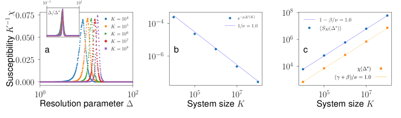
Figure S5: Finite-size scaling analysis of percolation in Poisson process. We use here $\mu=1$. (a) Susceptibility [i.e., Eq. (S7)] divided by $K$, as a function of the resolution parameter $\Delta$. The inset shows the same data as of the main panel but the resolution parameter is rescaled as $\Delta/\Delta^{*}$. (b) Convergence of the effective critical point to the critical point. We measure $\Delta^{*}(K)$ as the value of the resolution parameter where we observe the peak of the susceptibility. (c) Scaling of the peak of susceptibility (orange squares) and of the average size of the largest cluster (blue circles) at the effective resolution $\Delta^{*}$.

Also, we confirm the value of the critical exponents $\tau=\alpha=2$ and $\sigma=\sigma_{T}=1$ by studying the collapse of the cluster number on the scaling function $\mathscr{G}$ (Figure S6).

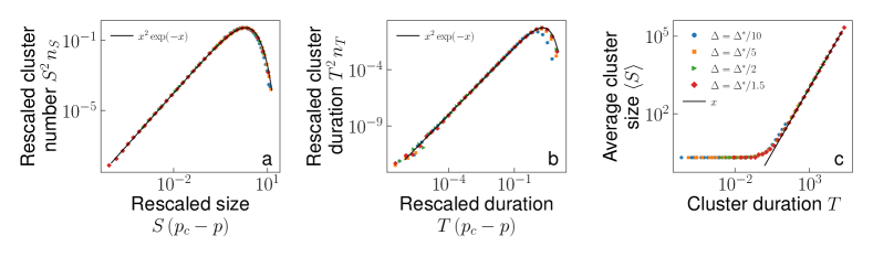
Figure S6: Cluster statistics of the Poisson process. We set $\mu=1$. Each curve is estimated by considering $C=10^{6}$ clusters. The system size is $K=10^{6}$. (a) Cluster number $n_{S}$, rescaled by $S^{2}$, as a function of $S(p_{c}-p)$, for different values of $p$ and $p_{c}=1$. Here, $p=1-e^{-\mu\Delta}$. The solid black line is the scaling function $\mathscr{G}(x)=x^{2}e^{-x}$ Stauffer and Jayaprakash (1978) (b) Cluster duration $n_{T}$, rescaled by $T^{2}$, as a function of $T(p_{c}-p)$. The solid black line is the same as in panel a. (c) Average size of clusters as a function of their duration. The black line indicates linear scaling.

We stress that the value of the critical exponent $\tau$ cannot be deduced immediately by looking at the distribution $P(S)$ at criticality (Figure S7).

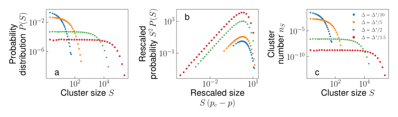
Figure S7: Cluster statistics of the Poisson process. We set $\mu=1$. Each curve is estimated by considering $C=10^{6}$ clusters. The system size is $K=10^{6}$. (a) Probability distribution $P(S)$ of the cluster size for different values of $\Delta$. (b) Same as in panel a, but the distribution is rescaled by $S^{2}$ and the ordinate is rescaled by $(p_{c}-p)$, with $p=1e^{-\mu\Delta}$ and $p_{c}=1$. (c) Cluster number $n_{S}$ for the same data as in panels a, b.

.5 Percolation theory of the critical Hawkes process

We can fully describe the percolation transition of the Hawkes process in terms of the percolation transition of the Poisson process. The only caveat is accounting for the fact that process is not stationary at criticality Hawkes and Oakes (1974). To this end, we simply assume that the process is a Poisson process with rate dependent on the number of events as in Eq. (S5). The effective critical point is

$$\Delta_{1}^{*}=\frac{\log(K)}{\langle{\lambda(K)}\rangle}=\frac{\log(K)}{\mu+\sqrt{2K\mu}}\,.$$

The above expression implies that, in the thermodynamic limit, the critical point of the model is $\Delta_{c}=0$ and that $\Delta_{1}^{*}$ approaches $\Delta_{c}$ with the exponent $\nu=2$ and a logarithmic correction. In Figure 1 of the main text, we have shown that the expression allows us to properly rescale the order parameter into a unique scaling function. The result is confirmed in Figure S8. The finding is compatible with the one valid for the homogeneous Poisson process. If the scaling of the threshold with system size is measured in units of time, we then recover $\nu=1$. In fact, the number of events scales quadratically with time, i.e., $k(t)\sim t^{2}$. There, the susceptibility associated to the order parameter collapses, if properly rescaled, on a unique curve, irrespective of the $\mu$ value under consideration. The empirical measure of the effective critical point, as the value of $\Delta$ where the susceptibility peaks, further shows the scaling $\Delta_{1}^{*}(K)\sim\log(K)/K^{1/2}$. The FSS analysis is completed by showing that the exponent $\beta=0$, as expected for a discontinuous transition, and that the exponent $\gamma=\nu$. It follows, from respectively Eqs. (S10) and (S11), that $\tau=2$ and $\sigma=2$.

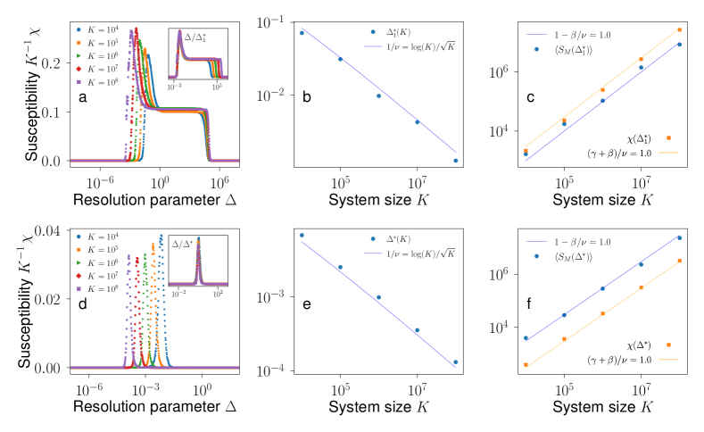
Figure S8: Finite-size scaling analysis of percolation in the Hawkes process. In panels a, b, and c, we use $\mu=10^{-4}$ . (a) Susceptibility [i.e., Eq. (S7)] divided by $K$ as a function of the resolution parameter $\Delta$. The inset shows the same data as in the main panel bu as a function of the rescaled variable $\Delta/\Delta_{1}^{*}$. (b) Scaling of the position of the peak of the susceptibility for different system size. (c) Scaling of the maximum of the susceptibility and of the average size of the largest cluster at the resolution $\Delta^{*}_{1}$. (d), (e), (f) Same as in panels a, b, and c, respectively, but for $\mu=10^{2}$.

The distribution of the cluster sizes and durations have been shown in Figure 2 of the main text. Figure S9 displays the complementary cumulative distribution for the same data in Figure 1 of the main text, confirming the results shown in the main text. Also, we display the linear scaling of the average size of clusters with given duration, as expected from the fact that both critical exponents $\tau=\alpha=2$. For $\mu\ll 1$ and $\Delta$ large enough, the cluster size distribution shows the scaling $\tau=3/2$. For this choice of the parameters, we observe also a quadratic relation between $S$ and $T$.

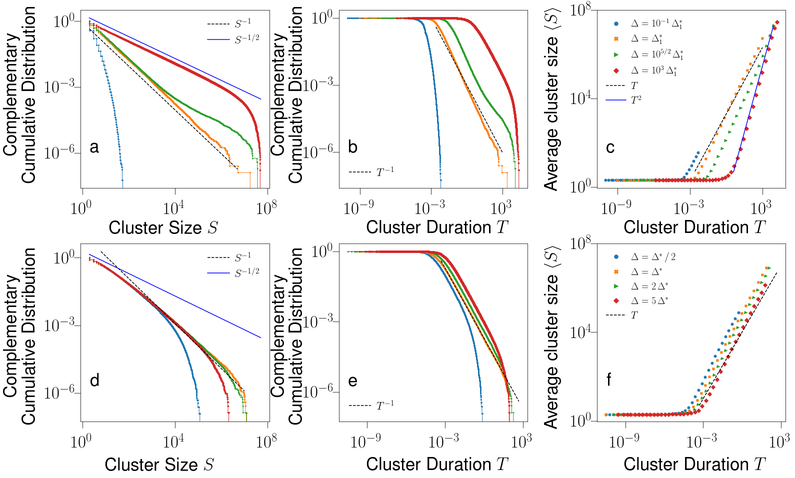
Figure S9: Critical percolation properties of self-exciting temporal processes. We consider the rate of Eq. (1) of the main text with exponential kernel function and $n=1$. System size is fixed at $K=10^{8}$. Histograms are obtained by considering $C=10^{7}$ clusters per configuration. We use $\mu=10^{-4}$ in panels a, b, and c. (a) Complementary Cumulative Distribution of the cluster size at different resolution $\Delta$. (b) Distribution of the cluster duration for the same data as in panel a. (c) Average size of clusters as a function of their duration for the same data as in panel (a). (d), (e) and (f) Same as in panels a, b, and c, respectively, but for $\mu=10^{2}$.

As stated in the main text, we further consider the power law kernel $\phi(x)=(\gamma-1)(1+x)^{-\gamma}$ for $\gamma>2$, so that $\phi(x)$ has a finite mean. The simulation requires the use of the thinning algorithm, so that the system size $K$ must be kept small. We show the percolation phase diagram and the cluster size distribution for both $\mu\ll 1$ and $\mu\gg 1$ in Fig. S10. The phenomenology is clearly analogous, with a double transition for $\mu\ll 1$ and a single transition for $\mu\gg 1$. Further, as Figure S4 shows, the rate grows again as the square root of the number of events, as expected for a branching process. It follows that the critical point $\Delta_{1}^{*}$ for the power-law kernel scales again as $K^{-1/2}$ as can be verified by rescaling the data in Figure S10a. Overall, Figure S4 and Figure S10 show that the results presented in the main text for the exponential kernel remain valid for the power law kernel which, in turn, suggests that the results are valid for any kernel with finite mean. Large-scale simulations of the non-Markovian Hawkes process can be performed by exploiting the map of the process with the branching process (BP), which is done in the next section.

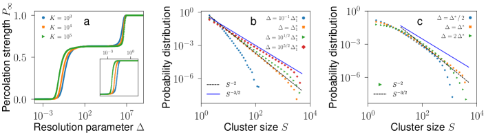
Figure S10: Percolation transition in power-law self-exciting temporal processes. We consider temporal processes generated by the rate of Eq. (1) of the main text with a power-law kernel and parameter $n=1$. The exponent of the power-law kernel is $\gamma=2.5$. Results are obtained by considering $R=10^{3}$ realizations of the process. (a) Percolation strength as a function of the resolution parameter. We display results for different system sizes $K$. In the main panel, we set $\mu=10^{-6}$. In the inset, results are obtained for $\mu=10^{2}$. (b) Distribution of the cluster size at criticality for $\mu=10^{-6}$. System size here is $K=10^{4}$. (c) Same as in panel b but for $\mu=10^{2}$.

.6 The temporal branching process

To numerically demonstrate the statistical equivalence between the Hawkes process and the branching process, in Figures S11 and S12 we show results valid for time series generated using a branching process with inter-event times respectively sampled from exponential and power-law distributions.

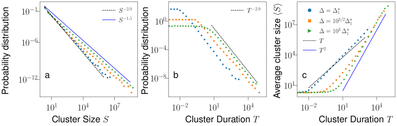
Figure S11: Critical percolation properties of time series generated from a branching tree with bonds weighted by inter-event times distributed as $\phi(x)$. We use here $\phi(x)=e^{-x}$. Histograms are obtained by considering $C=10^{6}$ clusters per configuration. (a) Distribution of the cluster size at different resolution $\Delta$. (b) Distribution of the cluster duration for the same data as in panel a. (c) Average size of clusters as a function of their duration for the same data as in panel a.

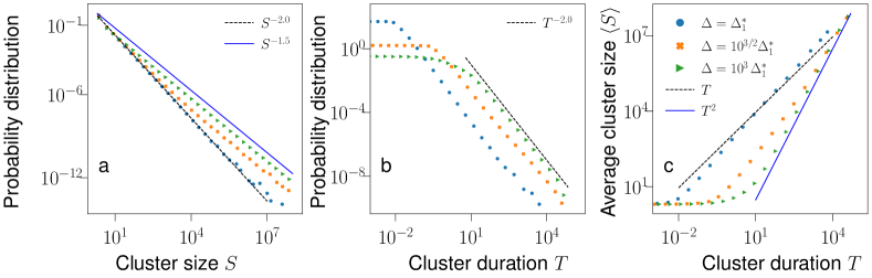
Figure S12: Critical percolation properties of time series generated from a branching tree with bonds weighted by inter-event times distributed as $\phi(x)$. We use here the power-law kernel $\phi(x)=(\gamma-1)(1+x)^{-\gamma}$ with $\gamma=2.5$. Histograms are obtained by considering $C=10^{6}$ clusters per configuration. (a) Distribution of the cluster size at different resolution $\Delta$. (b) Distribution of the cluster duration for the same data as in panel a. (c) Average size of clusters as a function of their duration for the same data as in panel a.

.7 Crossover point

As stated in the main text, the crossover between the scaling $\tau=2$ and $\tau=3/2$ can be understood as a threshold phenomenon due to the finite temporal resolution. According to the scaling argument of Eq. (2) the crossover is observed when clusters have size large enough for their duration to be comparable with $\Delta^{-1}$. On average, the largest cluster whose duration is $T\leq\Delta^{-1}$ has size $S_{T}\propto\Delta^{-1}T$ so that $S_{T}\leq\Delta^{-2}$. Analogously, the smallest cluster whose duration is $T\geq\Delta^{-1}$ has, on average, size $S_{T}\propto T^{2}$ so that $S_{T}\geq\Delta^{-2}$. It follows that the crossover point is expected to scale with the temporal resolution as $S_{c}\propto\Delta^{-2}$. This result is confirmed in Fig. S13a.

.8 System size and sample size

The argument further allows us to understand the properties of the cluster size distribution. Given the power-law shape of $P(S)$, the largest cluster in a sample of size $C$ grows as a power law Boguná et al. (2004). If $C$ is not large enough for (at least) the largest cluster to have size comparable with $\Delta^{-1}T$, then the power-law shape of $P(S)$ is not observed at all, and the distribution appears to be exponential. If the sample size is large enough, then $P(S)$ does not show any further dependence on $C$, and the crossover point $S_{c}$ is not affected by $C$, as confirmed by Figure S13b. Finally, for a given system size $K$, we have shown that there exist a pseudo-critical temporal resolution $\Delta_{1}^{*}(K)$ such that $P(S)\sim S^{-2}$. As $\Delta_{1}^{*}\rightarrow 0$, reducing $K$ for a given $\Delta$ is analogous to increasing $\Delta$ for a given $K$ (and vice versa). It follows that, for a given temporal resolution $\Delta$, system size can be too small for power-law scaling to be observed or large enough for the crossover between the two regimes to be observed. Between the two extremes, there exists a size such that the resolution $\Delta=\Delta_{1}^{*}(K)$, as shown in Figure S13c.

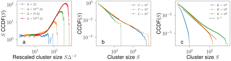
Figure S13: Crossover behavior and role of system and sample size in cluster statistics of the Hawkes process. We use $\phi(x)=e^{-x}$ and $\mu=10^{-4}$. (a) Complementary Cumulative Distribution Function (CCDF), rescaled by $S$, against the rescaled cluster size $S\Delta^{-2}$ of $C=10^{7}$ clusters. We use here $K=10^{8}$. (b) CCDF$(S)$ for different sample size $C$. We use here $\Delta=0.1954$ and $K=10^{8}$. (c) CCDF$(S)$ for different system size. We consider here $C=10^{7}$ clusters and $\Delta=0.0195$.

.9 Theory of critical branching process explains plateau values observed in phase diagrams

We show here that numerical values of the order parameter and susceptibility observed in Figure 1b of the main text, and Figures S8a, and S8d can be reproduced by considering the statistics of the critical branching process. Recall that the order parameter is obtained as the normalized size of the largest cluster, averaged over several realizations, and that the susceptibility is defined as the fluctuations of the average size of the largest cluster. We can reproduce these statistics by:

1. Extracting a sample of size $C$ of iid random variables $\{Z_{1},Z_{2},\ldots,Z_{C}\}$ from the power-law distribution $P(Z)\sim Z^{-3/2}$, i.e., the distribution of the tree size for a critical branching process.

2. Calculating their sum $V=\sum_{c=1}^{C}Z_{q}$ and their maximum $Z_{max}=\max\{Z_{1},Z_{2},\ldots,Z_{C}\}$ to estimate $Y=Z_{max}/V$. In this way $Y$ represents $S_{M}/K$ in a single realization of the Hawkes process. Order parameter and susceptibility can be obtained by averaging.

3. Repeating the first two points $T$ times to obtain the sample $\{Y_{1},Y_{2},\ldots,Y_{T}\}$, and finally estimating the order parameter as

   $$P_{\infty}=T^{-1}\sum_{t=1}^{T}Y_{t}$$

   and the susceptibility as

   $$\chi=\left(T^{-1}\sum_{t=1}^{T}Y^{2}_{t}-P_{\infty}^{2}\right)/P_{\infty}\;.$$

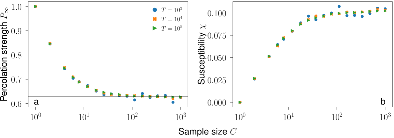
Figure S14: (a) Estimate of the order parameter $P_{\infty}$ as a function of the sample size $C$ obtained for different total realizations $T$ of the process. The horizontal black line stands for $P_{\infty}=1-1/e$. (b) Susceptibility $\chi$ as a function of the sample size. $\chi$ plateaus at the same value as observed in Figure 1b of the main text, and Figures S8a and S8d.

.10 Percolation theory of the subcritical Hawkes process

As stated in the main text, several different systems exhibit bursty patterns of activity. Neuronal networks are one possible example of such systems. Whether the brain truly operates at criticality Beggs and Plenz (2003) or in a slightly subcritical state Priesemann et al. (2014) is a debated argument. As such, it could be interesting to check whether the theory presented in the main text remains valid for $n\lesssim 1$.

We studied the percolation transition and the cluster distributions in the Hawkes process with exponential kernel and $n=0.95$. Results are coherently explained by the theory already used for the critical configuration. The long-term estimates of the first $\langle{\lambda}\rangle$ and second moment $\langle{\lambda^{2}}\rangle$ of the rate of an exponential Hawkes process in the subcritical regime $n<1$ are given again in Ref. Dassios and Zhao (2011). They read as

$$\begin{split}&\langle{\lambda}\rangle=\frac{\mu}{1-n}\\ &\langle{\lambda^{2}}\rangle=\frac{2\mu^{2}+n^{2}\mu}{2(1-n)^{2}}\,.\end{split}$$ (S14)

Both the above expressions are valid in the long-term limit, when the process is stationary. In particular, we note that the square of the ratio standard deviation over average value is inversely proportional to $\mu$, i.e.,

$$\frac{\langle{\lambda^{2}}\rangle-\langle{\lambda}\rangle^{2}}{\langle{\lambda}\rangle^{2}}=\frac{n^{2}}{2\mu}\,.$$ (S15)

The results of the numerical simulations reported in Figures S15 and S16 are explained using the above expressions.

For $\mu\ll 1$, the behavior is similar to the one observed for the critical Hawkes process. In this regime, time series consist of quick bursts of activity well separated in time. The fundamental difference with the critical configuration is that burst sizes obey a power-law distribution with a neat exponential cut-off Kossio et al. (2018). As such, the largest cluster generated by a single burst has finite size, independently of the system size $K$. In turn, the value of the plateau observed in the percolation phase diagram decreases as $K$ increase, and the associated phase transition disappears in the thermodynamic limit, see Figure S15. In finite-size systems, we can still measure the cluster distributions $P(S)$ and $P(T)$ around the pseudo-critical point $\Delta^{*}_{1}$, as done in Figure S16. The Poisson-like transition is observed at the pseudo-critical point $\Delta^{*}_{2}=\log(K)/\mu$. This second transition does not vanish as the system size increases.

For $\mu\gg 1$, Eq. (S15) tells us that fluctuations are much smaller than the expected value of the rate, so we expect the process to behave as a Poisson process with rate $\langle{\lambda}\rangle$. In particular, the phase diagram should look like the one of a homogeneous one-dimensional percolation model with occupation probability $p=1-e^{-\langle{\lambda}\rangle\Delta}$, thus consisting of a unique transition happening at $\Delta^{*}=\log(K)/\langle{\lambda}\rangle$. Our prediction is confirmed by the collapse of the order parameter shown in Figure S15c, and further supported by the numerical analysis regarding the scaling of the cluster number, see Figure S16.

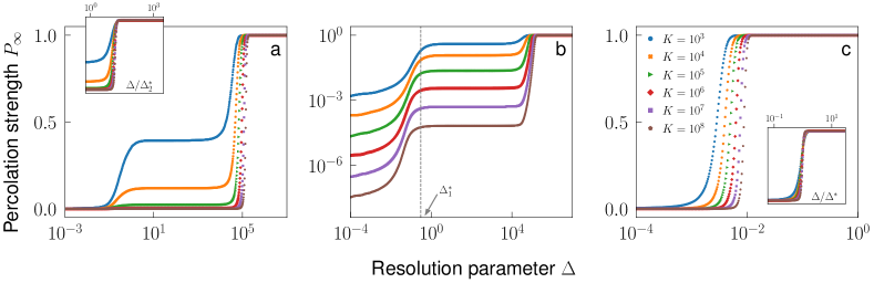
Figure S15: Percolation phase diagrams of the subcritical Hawkes process. We consider the exponential kernel function and use $n=0.95$. We plot the percolation strength $P_{\infty}$ as a function of the resolution parameter $\Delta$ for different configurations and different system sizes K. Average values are obtained by considering $R=10^{3}$ realizations of the process. (a) We set $\mu=10^{-4}$. The inset shows the same data as of the main panel but the resolution parameter is rescaled as $\Delta/\Delta^{*}_{2}$, with $\Delta^{*}_{2}=(1-n)\log(K)/\mu$. (b) Same as in panel a, but we use the logarithmic scale for the ordinates. The vertical gray line roughly indicates the position of the pseudo-critical point $\Delta^{*}_{1}$. We use this value as the reference for the plots in Figure S16. (c) We set $\mu=100$. The inset shows the same data as of the main panel but the resolution parameter is rescaled as $\Delta/\Delta^{*}$, with $\Delta^{*}=(1-n)\log(K)/\mu$.

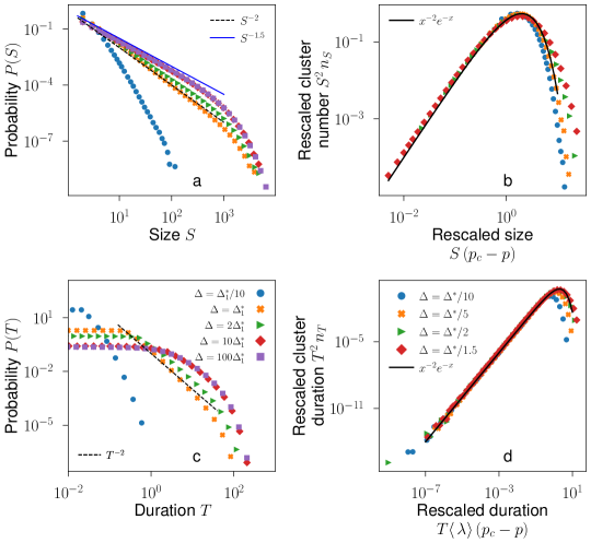
Figure S16: Percolation properties of the subcritical Hawkes process. We consider temporal processes identical to those studied in Figure S15, thus generated using an exponential kernel function with $n=0.95$. System size is fixed at $K=10^{8}$. Histograms are obtained by considering $C=10^{7}$ clusters per configuration. (a) We set $\mu=10^{-4}$. Probability density function of cluster size $S$ for different values of $\Delta$. The dashed black line scales as $S^{-2}$ while the solid blue line scales as $S^{-3/2}$. (b) We set $\mu=100$. Cluster number $n_{s}$, rescaled by $S^{2}$, as a function of $S(1-p)$, for different values of $p$. The solid black line is the scaling function $\mathscr{G}(x)=x^{2}e^{-x}$. (c) We set $\mu=10^{-4}$. Probability density function of cluster duration $T$ for different values of $\Delta$. The dashed black line scales as $T^{-2}$. (d) We set $\mu=100$. Cluster duration $n_{T}$, rescaled by $T^{2}$, as a function of $\langle{\lambda}\rangle T(1-p)$, for the same values of $p$ as in panel (a). The solid black line is the scaling function $\mathscr{G}(x)=x^{2}e^{-x}$.

.11 Non-homogeneous Poisson process with rate linearly growing in time

Here we discuss a non-homogeneous Poisson process with rate linearly growing in time, i.e., $\lambda(t)=t$. Numerical simulations of the model can be performed efficiently by using the inverse transform method. Specifically, the probability that no events are observed in the interval $(t,t+x)$ is

$$P_{n=0}[t,x]=\exp\left(-\int_{t}^{t+x}\lambda(t^{\prime})\,dt^{\prime}\right)\,.$$ (S16)

Thus, the inter-event time $x$ is a random variable satisfying

$$x=-t+\sqrt{t^{2}-2\log(u)}\,\text{, where }\,u\sim\text{Unif}(0,1)\,.$$ (S17)

All inter-events are obtained from the above expression, including the first one at $t=0$.

We note that $\lambda(t)=t$ implies that $k(t)=t^{2}$ and $\lambda(k)=\sqrt{k}$. Figure S17 shows that the expected dependence $k(t)=t^{2}$ is correct.

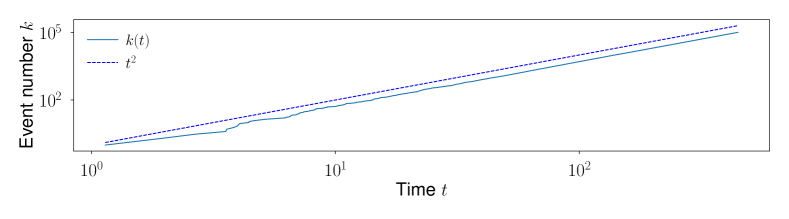
Figure S17: Individual realizations of the non-homogeneous Poisson process with deterministic linear time growth. The realization is made of $K=10^{5}$ events. The dashed blue line is the expected relation $k(t)=t^{2}$.

We remark that the most general expression for a linearly increasing rate is $\lambda(t)=\mu+\beta t$. In our experiments, we assume that time is measured in units equal to $\beta$. Further, we assume $\mu=0$. Taking $\mu>0$ would correspond to a minimal modification of Eq. (S17) having no significant impact on the results reported below.

Figure S18a shows the percolation strength as a function of the resolution parameter $\Delta$. The transition point of the model is expected to scale as $\Delta^{*}=\log(K)/\sqrt{K}$ for a time series with $K$ events. Such a prediction is verified in the inset of Figure S18a. The validity of the percolation framework is further confirmed in Figure S19a, where the susceptibility is shown to collapse under the usual rescaling of the temporal resolution, and in Figure S19b, where the location of the susceptibility’s peak is shown to converge to $0$ as $\Delta^{*}(K)=\log(K)/\sqrt{K}$. Figure S19c further displays the measure of the exponent $\beta=0$ and $\gamma=1$. Figures S18b and  S18c show the scaling properties of finite clusters, revealing that the process belongs to the universality class of 1D percolation, characterized by the exponents $\tau=\alpha=2$.

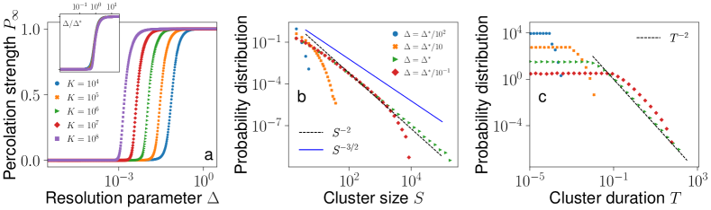
Figure S18: Percolation transition in the non-homogeneous Poisson processes. Results are obtained by considering $R=10^{3}$ realizations of the process. (a) Percolation strength as a function of the resolution parameter $\Delta$. We display results for different system sizes $K$. The inset shows the same data as of the main panel but the resolution parameter is rescaled as $\Delta/\Delta^{*}$. (b) Distribution of the cluster size. System size here is $K=10^{6}$. (c) Distribution of the cluster duration for the same data of panel (b).

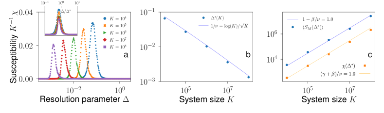
Figure S19: Finite-size scaling analysis of percolation in the non-homogeneous Poisson process.(a) Susceptibility [i.e., Eq. (S5)] divided by K, as a function of the resolution parameter $\Delta$. The inset shows the same data as of the main panel but the resolution parameter is rescaled as $\Delta/\Delta^{*}$. (b) Convergence of the effective critical point to the critical point. We measure $\Delta^{*}$ as the value of the resolution parameter where we observe the peak of the susceptibility. (c) Scaling of the peak of susceptibility (orange squares) and of the average size of the largest cluster (blue circles) at the effective resolution $\Delta^{*}$.

In conclusion, the non-homogeneous Poisson process with linearly increasing rate has the same critical properties as of the homogeneous Poisson process.