Feedback in Imitation Learning:
The Three Regimes of Covariate Shift

Abstract

Imitation learning practitioners have often noted that conditioning policies on previous actions leads to a dramatic divergence between “held out” error and performance of the learner in situ. Interactive approaches (Ross et al., 2011) can provably address this divergence but require repeated querying of a demonstrator. Recent work identifies this divergence as stemming from a “causal confound” (de Haan et al., 2019; Wen et al., 2020) in predicting the current action, and seek to ablate causal aspects of current state using tools from causal inference. In this work, we argue instead that this divergence is simply another manifestation of covariate shift, exacerbated particularly by settings of feedback between decisions and input features. The learner often comes to rely on features that are strongly predictive of decisions, but are subject to strong covariate shift.

Our work demonstrates a broad class of problems where this shift can be mitigated, both theoretically and practically, by taking advantage of a simulator but without any further querying of expert demonstration. We analyze existing benchmarks used to test imitation learning approaches and find that these benchmarks are realizable and simple and thus insufficient for capturing the harder regimes of error compounding seen in real-world decision making problems. We find, in a surprising contrast with previous literature, but consistent with our theory, that naive behavioral cloning provides excellent results. We detail the need for new standardized benchmarks that capture the phenomena seen in robotics problems.

1 Introduction

Figure 1: A common example of feedback-driven covariate shift in self-driving. At train time, the robot learns that the previous action (Brake) accurately predicts the current action almost all the time. At test time, when the learner mistakenly chooses to Brake, it continues to choose Brake, creating a bad feedback cycle that causes it to diverge from the expert.

Imitation learning (IL) is a method of training robot controllers using demonstrations from human experts. In contrast to, e.g., reinforcement learning (RL), IL controllers can learn to perform complex control tasks “offline”, without interaction in the environment, and achieve remarkable proficiency with relatively few demonstrations. This speedup comes at a cost, however, since offline learning in robotic control introduces feedback artifacts which must be accounted for.

Consider the problem of training a a self-driving car to stop at a yellow light, as depicted in Figure 1. When an expert human driver decides whether to throttle or Brake, they may pay attention to timing of the light, pedestrians, or their previous action. A robot trained to naively imitate this demonstration, however, will latch onto the previous action as it predicts the current action almost all the time. At test time, when the learner inevitably makes a mistake, this mistake feeds into the features for the next timestep. This starts a vicious cycle of errors, as the learner diverges from the expert, not having learned how to recover.

This driving scenario is a classic example of a feedback loop (Bagnell, 2016; Sculley et al., 2014) between the learners actions and the input features a learner sees. This effects results in a covariate shift between training data and the input data a learner encounters when it executes its own policy. This shift leads to often a dramatic divergence between “hold out“ error and performance of the learner actually executing the policy in situ. Feedback-driven covariate shift in the context of imitation learning was first observed by (Pomerleau, 1989) and has recently resurfaced as a often recurring problem in self-driving (Kuefler et al., 2017; Bansal et al., 2018; Codevilla et al., 2019). Imitation learner error in settings with explicit feedback is sometimes attributed to a causal confound (de Haan et al., 2019), however, we argue that it is simply a more visible case of feedback-driven covariate shift.

A common approach to address covariate shift in imitation learning is to interactively query an expert in states that the learner visits (Ross et al., 2011; Ross, 2013) using the DAgger algorithm. Consider a class of learner policies $\pi$ that can achieve a one-time-step classification error of $\epsilon$ with respect to the expert’s chosen action. Whereas naive behavioral cloning (BC) suffers a classification regret of $O(T^{2}\epsilon)$ that grows quadratically in horizon $T$, interactive imitation learning approaches like DAgger guarantee the optimal $O(T\epsilon)$ regret even in the worst case. However, interactively querying experts is impractical in many cases where human experts are unable to provide feedback online.

Although interactive methods are provably necessary in the worst case, we posit that there are many problems with more modest demands in a “Goldilocks Regime” of moderate difficulty that can be solved without the need for an interactive expert. We propose solving those problems in a modified imitation learning setting where we have access to a fixed set of cached expert demonstrations as well as generative access to a high fidelity simulator of the environment. This is similar to inverse reinforcement learning settings that benefit from environment/simulator access during the process of training (Abbeel & Ng, 2004; Ziebart et al., 2008; Ho & Ermon, 2016; Finn et al., 2016) In this setting, we introduce a novel class of algorithms that provably address feedback-driven covariate shift.

Our key insight is that, as long as the expert demonstrator visits all states that the learner will visit, then the density ratio between the expert and learner is bounded, $P_{\textrm{learner}}(s)/P_{\textrm{expert}}(s)\leq C$, we can correct for the covariate shift and enjoy a regret of just $O(\epsilon T)$ using just a simulator and cached demonstrations.

Our contributions are the following:

1. We introduce a general framework for mitigating covariate shift using cached expert demonstrations, called ALICE (Aggregate Losses to Imitate Cached Experts)

2. We propose a family of loss functions within that framework and analyze their consistency.

3. We identify specific characteristics needed for better benchmarks in imitation learning.

2 Preliminaries: The Feedback Problem

For simplicity, we consider an episodic finite-horizon Markov Decision Process (MDP) $\left\langle\mathcal{S},\mathcal{A},C,P,\rho,T\right\rangle$ where $\mathcal{S}$ is a set of states, $\mathcal{A}$ is a set of actions, $C:\mathcal{S}\rightarrow[0,1]$ is a (potentially unobserved) state-dependent cost function, $P:\mathcal{S}\times\mathcal{A}\rightarrow\Delta(\mathcal{S})$ is the transition dynamics, $\rho\in\Delta(\mathcal{S})$ is the initial distribution over states, and $T\in\mathbb{N}^{+}$ is the time horizon. Given a policy $\pi:\mathcal{S}\rightarrow\Delta(\mathcal{A})$, let $\rho_{\pi}^{t}$ denote the distribution over states at time $t$ following $\pi$. Let $\rho_{\pi}$ be the average state distribution $\rho_{\pi}=\frac{1}{T}\sum_{t=1}^{T}\rho_{\pi}^{t}$. Let $Q^{\pi}$ be the cost-to-go for selecting $a$ at $s$ and following $\pi$ thereafter, $Q^{\pi}_{t}(s,a)=C(s)+\mathbb{E}_{s\sim P(s,a)}\left[C(s^{\prime})\right]+\sum_{t^{\prime}=t+1}^{T-1}\mathbb{E}_{s^{\prime\prime}\sim P(s_{t^{\prime}},\pi(s_{t^{\prime}}))}\left[C(s^{\prime\prime})\right]$. Let the (dis)-advantage function $A^{\pi}$ be the difference in cost-to-go between selecting action $a$ and selecting action $\pi(a)$, $A^{\pi}(s,a)=Q^{\pi}(s,a)-Q^{\pi}(s,\pi(s))$. The total cost of executing policy $\pi$ for $T$-steps is $J(\pi)=\sum_{t=1}^{T}\mathbb{E}_{s_{t}\sim\rho_{\pi}^{t}}\left[C(s_{t})\right]=T\mathbb{E}_{s\sim\rho_{\pi}}\left[C(s)\right]$.

In imitation learning, we do not observe $C(s)$. Instead, we observe only cached expert demonstrations $\mathcal{D}_{\mathrm{exp}}=\{(s_{t}^{*},a_{t}^{*})\}$ generated a priori by the expert $\pi^{*}$, i.e, $s_{t}^{*}\sim\rho_{\pi^{*}}^{t},a_{t}^{*}\sim\pi^{*}(.|s_{t}^{*})$. The cost $C(s)$ can be constructed as a “mismatch” loss relative to the expert (i.e. 0-1 classification loss for discrete actions or squared error in state or action for continuous spaces). Whether $C(s)$ is set by the MDP or relative to the expert, the analysis is the same, and the goal is to train a policy $\pi$ that minimizes the performance difference $J(\pi)-J(\pi^{*})$ via imitation. When $C(s)$ is a loss relative to the expert, minimizing performance difference is equivalent to minimizing on-policy expert mismatch.

$$J(\pi)-J(\pi^{*})=T\mathbb{E}_{s\sim\rho_{\pi}}\left[\mathbbm{1}_{\pi(s)\neq\pi^{*}(s)}\right]$$

Feedback Drives Covariate Shift

The traditional approach to imitation learning, Behavior Cloning (BC) (Pomerleau, 1989), simply trains a policy $\pi$ that correctly classifies the expert actions on a cached set of demonstrations:

$$\hat{\pi}=\underset{\pi\in\Pi}{\operatorname*{arg\,min}}\;\mathbb{E}_{(s^{*},a^{*})\sim\mathcal{D}_{\mathrm{exp}}}\left[\ell^{\mathrm{cs}}(\pi(s^{*}),a^{*})\right].$$ (1)

where $\ell^{\mathrm{cs}}$ is a classification loss. Here, the best we could hope for is to drive down the training error $\mathbb{E}_{(s^{*},a^{*})\sim\mathcal{D}_{\mathrm{exp}}}\left[\ell^{\mathrm{cs}}(\hat{\pi}(s^{*}),a^{*})\right]\leq\epsilon$ and ensure a similar validation error on held out data. This is perfectly reasonable in the supervised learning setting where low hold-out error implies low test error.

However, sequential decision making tasks contain inherent feedback, where past action $a_{t-1}$ affect the input to our learner’s decision making at time $t$. As shown in the graphical model in Fig. 2, this can happen through multiple channels. It can happen indirectly through the MDP dynamics where $a_{t-1}$ affects $s_{t}$, and can also happen explicitly when $\pi$ is directly conditioned on previous actions, i.e. $\pi(a_{t}|s_{t},a_{t-1})$. In fact, dependence on past actions is often essential to ensure model smoothness or hysteresis.

Figure 2: Inherent feedback in sequential decision making tasks. Past action $a_{t-1}$ affects current action $a_{t}$, either indirectly (blue) via MDP dynamics or directly (green) via explicit conditioning.

A commonly observed phenomena (Pomerleau, 1989; Ross & Bagnell, 2010; Brantley et al., 2019) is that such feedback loops drive covariate shift, where the states experienced by the learner $s_{t}\sim\rho_{\pi}^{t}$ diverge significantly from $\mathcal{D}_{\mathrm{exp}}$. Although a learner begins by making an error of just $\epsilon$, those errors drive the learner into novel states rarely demonstrated by the expert where it is even more likely to make mistakes. Distributional shift and compounding errors result in total error $O(T^{2}\epsilon)$. This is formalized below:

Theorem 1 (Theorem 2.1 in (Ross et al., 2011)).

Let $\mathbb{E}_{s\sim\rho_{\pi}}\left[\ell^{\mathrm{cs}}(\hat{\pi}(s),\pi^{*}(s))\right]\leq\epsilon$ be the bounded on-policy training error, where $\ell^{\mathrm{cs}}$ is the 0-1 loss (or an upper bound). We have $J(\hat{\pi})\leq J(\pi^{*})+T^{2}\epsilon$

(Ross et al., 2011) go on to show that it is possible to achieve the ideal $O(T\epsilon)$ error by interactively querying the expert on states visited by the learner $s\sim\rho_{\pi}$, and minimizing the same classification loss $\ell^{\mathrm{cs}}$.

Theorem 2 (Theorem 2.2 in (Ross et al., 2011)).

Let $\mathbb{E}_{s\sim\rho_{\pi}}\left[\ell^{\mathrm{cs}}(\hat{\pi}(s),\pi^{*}(s))\right]\leq\epsilon$ be the bounded on-policy training error, and $A^{\pi^{*}}(s,a)\leq u$ be the bounded (dis)-advantage w.r.t expert $\forall s,a$. We have $J(\hat{\pi})\leq J(\pi^{*})+uT\epsilon$.

However, querying the expert online is impractical in many settings (Laskey et al., 2017), requiring a human to provide cognitively challenging low-latency open-loop controls. This inspires a search for methods which achieve similar bounds without the need for an interactive demonstrator, asking the following question:

Problem 1.

Can we achieve $O(T\epsilon)$ error without querying the expert online, i.e., using only the cached expert $\mathcal{D}_{\mathrm{exp}}$?

3 Confusion on Causality and Covariate Shift

We now take a slight detour to review instances where feedback causes real problems in imitation learning for self-driving, and clarify a widespread confusion between covariate shift and causality. A common observation in all these instances is that while past actions are strongly correlated with future actions, it often leads to a latching effect where once the robot begins to brake, it continues braking.  (Muller et al., 2006) first note such correlations this with steering actions, but more recently (Kuefler et al., 2017; Bansal et al., 2018; de Haan et al., 2019) note this with braking actions and  (Codevilla et al., 2019) note a correlation between speed and desired acceleration.

In an important paper, (de Haan et al., 2019) look to understand the problem of feedback through the lens of causal reasoning (Pearl et al., 2016; Spirtes et al., 2000). They note that, practically, the most severe repercussions come from features that enable the learner to condition almost directly on previous actions. The authors propose that: “This situation presents a give-away symptom of causal misidentification: access to more information leads to worse generalization performance in the presence of distributional shift. Causal misidentification occurs commonly in natural imitation learning settings, especially when the imitator’s inputs include history information.” and that their contribution is: “We propose a new interventional causal inference approach suited to imitation learning.”

Fig. 2 shows the graphical model under consideration. The authors claim $z_{t}=[s_{t-1},a_{t-1}]$ is a confounder between the independent variable $s_{t}$ and the dependent variable $a_{t}$. However, $z_{t}$ is fully observed. From  (Pearl et al., 2016) (Theorem 3.2.2), $s_{t}$ and $a_{t}$ are not confounded iff $P(a_{t}|\mathrm{do}(s_{t}))=P(a_{t}|s_{t})$, i.e. whenever the observationally witnessed association between them is the same as the association that would be measured in a controlled experiment, with $s_{t}$ randomized. In the experimental setups they considered, despite explicit conditioning on previous actions we failed to find true confounders as all variables are observed.

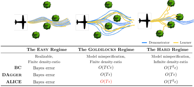
Figure 3: Spectrum of feedback driven covariate shift regimes. Consider the case of training a UAV to fly through a forest using demonstrations (blue). In Easy regime, the demonstrator is realizable, while in the Goldilocks and Hard regime, the learner (yellow) is confined to a more restrictive policy class. While model mispecification usually requires interactive demonstrations, in the Goldilocks regime, ALICE achieves $O(T\epsilon)$ without interactive query.

When all variables are observed, under infinite data regime and full support (all modes excited), behavior cloning / MLE is consistent. Indeed (Zhang et al., 2020) similarly prove that “if the expert and learner share the same policy space, then the policy is always imitable”. While the authors of (de Haan et al., 2019) claim “We define causal misidentification as the phenomenon whereby cloned policies fail by misidentifying the causes of expert actions”, we posit that this is not a causal issue but rather one of finite data regime and/or model misspecification. The learner prediction error $\epsilon$ concentrates unevenly as the learner comes to rely on a features that are strongly predictive of actions, but create strong feedback loops that lead to covariate shift.

Finally, if we alter the graphical model to have an unobserved casual confounders, (de Haan et al., 2019) is correct to note that this would manifest as a covariate shift and lead to poor performance even in the infinite data limit. However, their proposed approach requires expert intervention similar to DAgger (although is can be much more sample efficient), which makes it difficult to apply in our setting. Instead, we propose to measure the induced covariate shift and directly adjust for it.

4 Feedback Driven Covariate Shift Spectrum

We return to Problem 1 – achieve $O(T\epsilon)$ error without repeatedly querying the expert. We adopt the large-sample, reduction-style analysis of (Beygelzimer et al., 2008; Ross & Bagnell, 2010; Ross et al., 2011) and for simplicity consider the infinite data regime to keep the focus squarely on understanding the error-compounding problem so common in real-world applications (Section 3).

While the theoretical analysis demonstrates that BC must incur $O(T^{2}\epsilon)$ error in the worst-case, practitioners have often noted settings where behavior cloning is effective (Bojarski et al., 2016). This suggests that there maybe varying regimes of difficulty in the imitation learning problem that call for different algorithmic assumptions and approaches as shown in Fig. 3

4.1 The Easy Regime: Realizable

In the simplest case, the expert is realizable $\pi^{*}\in\Pi$. We can simply drive the classification error to $\epsilon=0$, recovering the expert policy. The prescription in this regime is the easiest practically and often quite powerful: collect as much data as possible and ensure realizability with a sufficiently broad policy class.

Crucially, we note theoretically and demonstrate below empirically that the benchmarks used in recent imitation learning literature (Ho & Ermon, 2016; Barde et al., 2020) all fall into the Easy regime. Without restrictions on model class, we find that the commonly used benchmarks are well solved by naive behavioral cloning and fail to capture real-world issues (Sculley et al., 2014; Pomerleau, 1989; Kuefler et al., 2017; Bansal et al., 2018; Codevilla et al., 2019). We suggest the methodological issues that may have led to prior beliefs that these benchmarks captured error-compounding and suggest improvements for future benchmarks.

4.2 The Hard Regime: Model Misspecification, Infinite Density-ratio

This is the hardest case, where the expert is not realizable, $\pi^{*}\notin\Pi$, and does not visit every state, thus leading to infinite learner-expert density ratio. As (Ross et al., 2011) note, when a fundamental limit (of $\epsilon$ classification error) is imposed on how accurately we can learn the expert’s policy whether due to partial observability, optimization limitations, or regularization, a compounding error of $O(T^{2}\epsilon)$ is simply inevitable without repeated access and interaction with the demonstrator. Interaction with the demonstrators enables the learner to achieve the best possible $O(T\epsilon)$ error. This comes fundamentally from the fact that there may simply be states that are never visited under the demonstrator policy and thus there is effectively no way to recover if an error leads our learner to such states. As such, interactive methods like DAgger (Ross et al., 2011) are inevitably required to achieve high performance.

4.3 The Goldilocks Regime: Model Misspecification, Finite Density-ratio

Consider now a regime where the expert is not realizable, $\pi^{*}\notin\Pi$, and there thus exists some inevitable classification error (captured crudely via the $\epsilon$ bound), but for which there is sufficient exploration in the data collected by observing the demonstrator that we can hope to learn good “recovery” behavior. We quantify that notion of exploration by saying that the demonstrator visits all states with some small probability, thus bounding the learner-demonstrator density ratio $\left|\left|{\rho_{\hat{\pi}}}/{\rho_{\pi^{*}}}\right|\right|_{\infty}\leq C$. We denote this the Goldilocks regime as we speculate this model is “just right” to capture much of the error compounding difficulty seen in real-world imitation learning.

We begin by noting that due to misspecification, a naive BC can still only provide sub-optimal performance $O(TC\epsilon)$.

Theorem 3 (BC in Goldilocks regime).

Let $\hat{\pi}$ be the learnt policy such that $\mathbb{E}_{(s^{*},a^{*})\sim\mathcal{D}_{\mathrm{exp}}}\left[\ell^{\mathrm{cs}}(\hat{\pi}(s^{*}),a^{*})\right]\leq\epsilon$. For bounded density ratio $\left|\left|{\rho_{\hat{\pi}}}/{\rho_{\pi^{*}}}\right|\right|_{\infty}\leq C$ and bounded (dis)-advantage $A^{\pi^{*}}(s,a)\leq u\;\forall(s,a)$, we have

$$J(\hat{\pi})\leq J(\pi^{*})+\min(TCu\epsilon,T^{2}\epsilon)$$ (2)

Proof.

See appendix A.1 ∎

In this regime, the problem becomes one of deploying finite model resources to lead to as good as possible performance. We approach Problem 1 from a perspective of covariate-shift correction and provide, for the first time to our knowledge, an approach that achieves $O(T\epsilon)$ without interactively querying the expert.

5 Approach

We speculate that the Goldilocks regime is relatively common in real-world applications and that in the large data limit the need to re-query an expert may be relatively uncommon. Although an interactive expert is sufficient to address this issue, we believe that only a set of cached expert demonstrations is necessary. We thus consider the use of classical covariate-shift mitigation strategies, though the IL setting introduces a complication. Due to feedback we have a subtle chicken-or-egg problem: high-performance covariate shift mitigation strategies rely on samples from the distribution of inputs (states) from the test distribution. However, the test distribution here is directly an effect of decisions made earlier by the policy.

We show how this can be addressed both for non-stationary and for stationary policies. For non-stationary policies (Sec 5.1), we use sequential forward training of successive policies. For stationary policies (Sec 5.3), we use an iterative approach which refines both policy and mitigation strategy until they stabilize.

We present ALICE (Aggregate Losses to Imitate Cached Experts), a family of algorithms that train a policy to imitate cached expert while countering or adjusting for covariate shift. Abstractly, all variants of ALICE optimize:

$$\hat{\pi}=\underset{\pi\in\Pi}{\operatorname*{arg\,min}}\;\ell(\pi,\mathcal{D}_{\mathrm{exp}},\Sigma)$$ (3)

where the loss $\ell(.)$ uses both cached demonstrations $\mathcal{D}_{\mathrm{exp}}$ and a simulator $\Sigma:\pi\mapsto\rho_{\pi}(s)$ to build the induced density $\rho_{\hat{\pi}}(s)$. There exist several choices for the loss $\ell(.)$ of which we analyze three, and show that they all lead to an $O(T\epsilon)$ bound under varying assumptions.

5.1 Forward Training Non-Stationary Policies

A simple resolution to the chicken-or-egg problem in (3) is to train a different policy $\hat{\pi}_{t}$ for every timestep. This leads to a simple, recursive recipe: at each time $t$, roll-in trained policies $\hat{\pi}_{1},\dots,\hat{\pi}_{t-1}$ in the simulator $\Sigma$ to construct $\rho_{\hat{\pi}}^{t}(s)$ and solve

$$\hat{\pi}_{t}=\underset{\pi\in\Pi}{\operatorname*{arg\,min}}\;\ell_{t}(\pi,\mathcal{D}_{\mathrm{exp}},\rho_{\hat{\pi}}^{t})$$ (4)

While training non-stationary policies is at times impractical, we use this setting to theoretically analyze various loss functions $\ell(.)$, deferring to Section 5.3 for a simple online variant with no fixed horizon.

5.2 Family of ALICE Loss Functions

We analyze two different losses – reweigh expert demonstrations by estimating the learner-expert density ratio, and match next state moments of learner-expert distribution. We also analyze a third loss that combines both ideas to be doubly robust.

Loss 1 (ALICE-Cov): Reweigh by Density Ratio

A classic approach to covariate shift mitigation (Shimodaira, 2000) is to reweigh samples by the density ratio of the target (learner) to the observed (expert) distribution.

$$\begin{split}\ell_{t}(\pi,\mathcal{D}_{\mathrm{exp}},&\rho_{\hat{\pi}}^{t})=\\ &\underset{s^{*}_{t},a^{*}_{t}\sim\mathcal{D}_{\mathrm{exp}}}{\mathbb{E}}\left[\left(\frac{\rho_{\hat{\pi}}^{t}(s^{*}_{t})}{\rho_{\pi^{*}}^{t}(s^{*}_{t})}\right)\ell^{\mathrm{cs}}(\pi(s_{t}^{*}),a_{t}^{*}))\right]\end{split}$$ (5)

where $\ell^{\mathrm{cs}}(.)$ is the plain classification loss. In practice, the density ratio is not known and must be estimated $\hat{r}(s)\approx\left(\frac{\rho_{\hat{\pi}}^{t}(s^{*}_{t})}{\rho_{\pi^{*}}^{t}(s^{*}_{t})}\right)$. ALICE-Cov is the simplest variant that requires only that the ratio estimate be bounded to guarantee $O(T\epsilon)$

Theorem 4 (ALICE-Cov).

Let $\hat{\pi}$ be the learned policy produced by ALICE-Cov such that $\ell_{t}(\hat{\pi},\mathcal{D}_{\mathrm{exp}},\rho_{\hat{\pi}}^{t})\leq\epsilon$. Let $\hat{r}(s_{t})$ be the density ratio estimate such that $\mathbb{E}_{s^{*}_{t}\sim\mathcal{D}_{\mathrm{exp}}}\left[\hat{r}(s_{t})-\frac{\rho_{\hat{\pi}}^{t}(s_{t})}{\rho_{\pi^{*}}^{t}(s_{t})}\right]\leq\gamma$. Let $A^{\pi^{*}}(s,a)\leq u\;\forall(s,a)$ be a bound on the (dis)-advantage w.r.t expert. We have

$$J(\hat{\pi})\leq J(\pi^{*})+Tu(\epsilon+\gamma)$$ (6)

Proof.

See appendix  A.2 ∎

Corollary 5.1.

Let $C(s)$ be the classification loss $\ell^{\mathrm{cs}}(\pi(s),\pi^{*}(s))$ with respect to expert and $\hat{\pi}$ be a policy produced as in Theorem. 4. In this case

$$J(\hat{\pi})\leq J(\pi^{*})+T(\epsilon+\gamma)$$ (7)

Proof.

For $C(s)=\ell^{\mathrm{cs}}(\pi(s),\pi^{*}(s))$, we have $u=1$. ∎

We incur a penalty $u$ in Theorem. 4 because we are matching expert actions via $\ell^{\mathrm{cs}}(.)$ instead of matching values, i.e. minimizing the expert dis-advantage function. We look at how to do this next.

Loss 2 (Fail): Match next-state moments

Since our ultimate objective is to match the expert’s value function, we can perhaps do so more effectively by matching moments of that function rather than matching individual actions. The loss function introduced in the Fail algorithm (Sun et al., 2019) does exactly that, matching moments of the expert and learner’s next state distribution $\rho_{t+1}$ for non-stationary policies. We reintroduce that loss here within our general framework, and combine it with covariate shift correction in the next section. Please refer to (Sun et al., 2019) for the full implementation details of Fail.

Assuming value functions $V^{*}_{t+1}(s)$ belong to a class of moments $\mathcal{F}_{t+1}:\mathcal{S}\rightarrow$, the learner can try to match the expert’s moments of the next state. An example of a metric that captures deviation from matching moments is the integral probability metric, where an adversary searches for a moment function $f\in\mathcal{F}_{t+1}$ that maximizes learner-expert moment mismatch. Given a learner distribution $\rho_{t}$ and expert distribution $\rho^{*}_{t+1}$, we can define the following IPM metric:

$$d(\pi|\rho_{t},\rho^{*}_{t+1})=\max_{f\in\mathcal{F}_{t+1}} \underset{\begin{subarray}{c}s_{t}\sim\rho_{t}\\ a_{t}\sim\pi\\ s_{t+1}\sim P(.|s_{t},a_{t})\end{subarray}}{\mathbb{E}}\left[f(s_{t+1})\right]$$ (8)

$$-\underset{s^{*}_{t+1}\sim\rho^{*}_{t+1}}{\mathbb{E}}\left[f(s^{*}_{t+1})\right]$$

where the first term is the the expected moment on states obtained by rolling out $\pi$ and the second term is the expected expert moment. Fail defines the loss as:

$$\ell_{t}(\pi,\mathcal{D}_{\mathrm{exp}},\rho_{\hat{\pi}}^{t})=d(\pi|\rho_{\hat{\pi}}^{t},\mathcal{D}_{\mathrm{exp}})$$ (9)

While Fail does not require a bounded density ratio to remove error compounding, it does require a different, at times stronger condition – the notion of one-step recoverability

Definition 5.1 (One-step Recoverability).

For any state distribution $\rho_{t}$, there exists a policy $\pi$ that bounds $d(\pi|\rho,\mathcal{D}_{\mathrm{exp}})\leq\epsilon$.

This basically requires that no matter what the current distribution, the learner can recover in a single time-step to drive the loss to $\epsilon$. Without this condition, divergences at earlier time-step could be unrecoverable and hence compound over time leading to $O(T^{2}\epsilon)$. When considering any IL method where $C(s)$ and corresponding value function $V^{*}(s)$ are inherent to the MDP (rather than relative to the expert as in $C(s)=\ell^{\mathrm{cs}}(\pi,s)$), recoverability becomes a fundamental requirement. If the environment includes hard branches between high and low reward paths, bounds on lost reward ($\epsilon$ here, $u$ in DAgger) becomes arbitrarily large since optimal actions are useless after an initial mistake. These requirements of recoverability can be thought of as imposing a limit on the reward “branchiness” of the environment, which we require here only in expectation. This is illustrated in Appendix A.5. With this condition, we have:

Theorem 5 (Fail).

Let $\hat{\pi}$ be the learnt policy produced by Fail such that $\ell_{t}(\hat{\pi},\mathcal{D}_{\mathrm{exp}},\rho_{\hat{\pi}}^{t})\leq\epsilon$, assuming the expert is one-step recoverable, and $\epsilon_{\mathrm{be}}$ be the Inherent Bellman Error (IBE). We have:

$$J(\hat{\pi})\leq J(\pi^{*})+2T(\epsilon+\epsilon_{\mathrm{be}})$$ (10)

Proof.

We require small IBE to account for the richness of the chosen function class $\mathcal{F}$ and its ability to realize $V^{*}$. See appendix  A.3 for proof and definition of IBE. ∎

Loss 3 (ALICE-Cov-Fail): Doubly robust loss

When we combine Loss 1 and 2, we still require a version of recoverability (captured completely in the loss bound $\epsilon$), but we can eliminate dependence on dis-advantage and IBE. We consider the following loss:

$$\begin{split}\ell_{t}(\pi,&\mathcal{D}_{\mathrm{exp}},\rho_{\hat{\pi}}^{t})=\\ &\underset{s^{*}_{t},a^{*}_{t}\sim\mathcal{D}_{\mathrm{exp}}}{\mathbb{E}}\left[\left(\frac{\rho_{\hat{\pi}}^{t}(s^{*}_{t})}{\rho_{\pi^{*}}^{t}(s^{*}_{t})}\right)\ell^{\mathrm{ipm}}(\pi(s^{*}),a^{*})\right]\end{split}$$ (11)

where

$$\ell^{\mathrm{ipm}}(\pi(s^{*}),a^{*})=\max_{f\in\mathcal{F}_{t+1}} \underset{\begin{subarray}{c}a_{t}\sim\pi(.|s^{*}_{t})\\ s_{t+1}\sim P(.|s^{*}_{t},a_{t})\end{subarray}}{\mathbb{E}}\left[f(s_{t+1})\right]$$ (12)

$$- \underset{\begin{subarray}{c}a^{*}_{t}\sim\pi(.|s^{*}_{t})\\ s^{*}_{t+1}\sim P(.|s^{*}_{t},a^{*}_{t})\end{subarray}}{\mathbb{E}}\left[f(s^{*}_{t+1})\right]$$

Comparing with ALICE-Cov (5), we swap out the classification loss $\ell^{\mathrm{cs}}(.)$ with next state IPM loss $\ell^{\mathrm{ipm}}(.)$. We have the following performance guarantee:

Theorem 6 (ALICE-Cov-Fail).

Let $\hat{\pi}$ be the learnt policy produced by ALICE-Cov-Fail such that $\ell_{t}(\hat{\pi},\mathcal{D}_{\mathrm{exp}},\rho_{\hat{\pi}}^{t})\leq\epsilon$. Let $\hat{r}(s)$ be the density ratio estimate such that $\mathbb{E}_{s^{*}_{t}\sim\mathcal{D}_{\mathrm{exp}}}\left[\hat{r}(s)-\frac{\rho_{\hat{\pi}}^{t}(s)}{\rho_{\pi^{*}}^{t}(s)}\right]\leq\gamma$. Let $A^{\pi^{*}}(s,a)\leq u\;\forall(s,a)$ be a bound on the (dis)-advantage w.r.t expert. We have

$$J(\hat{\pi})\leq J(\pi^{*})+T(\epsilon+u\gamma)$$ (13)

Proof.

See appendix  A.4. ∎

If the density ratio estimate is perfect, $\gamma=0$, the bound is $O(T\epsilon)$, i.e. we have no dependence on $u$.

5.3 Iterative Training Stationary Policies

We now provide a more practical variant of ALICE that trains a single stationary policy. We use the same principle in (Ross et al., 2011) to reduce the chicken-or-egg problem to an iterative no-regret online learning (Shalev-Shwartz & Kakade, 2008), for example, via dataset aggregation.

Algorithm 1 provides an outline. It takes in a dataset of cached expert demonstrations $\mathcal{D}_{\mathrm{exp}}$ and a simulator. At iteration $i$, it rolls in the current learner $\hat{\pi}^{i}$ via the simulator to construct the learner state distribution $s_{t}\sim\rho_{\hat{\pi}^{i}}^{t}$ for any timestep. This in turn is used to compute a dataset of losses across various timesteps. This dataset is then aggregated with previous datasets and a new learner $\pi^{i+1}$ is computed on the whole dataset. For strongly convex losses, Algorithm 1 is a no-regret online algorithm, and hence achieves sub-linear regret against the best policy in hindsight. With some regularization, we can recover an algorithm $O(T\epsilon)$ with any of the 3 losses.

Algorithm 1 ALICE

  Input: Cached expert demonstrations $\mathcal{D}_{\mathrm{exp}}=\{(s_{t}^{*},a_{t}^{*})\}$, Simulator $\Sigma:\pi\rightarrow\rho_{\pi}$

  Initialize dataset $\mathcal{D}\leftarrow\emptyset$

  Initialize learner $\hat{\pi}^{1}$ to any policy in $\Pi$

  for $i=1$ to $N$ do

     Sample states $s_{t}\sim\rho_{\hat{\pi}^{i}}^{t}$ by running $\hat{\pi}^{i}$ in simulator $\Sigma$

     Compute a dataset of losses $\mathcal{D}_{i}=\{\ell_{t}(\pi,\mathcal{D}_{\mathrm{exp}},\rho_{\hat{\pi}^{i}}^{t})\}$.

     Aggregate datasets: $\mathcal{D}\leftarrow\mathcal{D}\bigcup\mathcal{D}_{i}$

     Train learner $\hat{\pi}^{i+1}$ on aggregated $\mathcal{D}$

  end for

  Return best $\hat{\pi}^{i}$ on validation

6 Evaluation and Benchmarks

In this section we take the opportunity to raise broader concerns with the benchmarks commonly used in imitation learning and identify necessary attributes of better benchmarks.

We performed a set experiments using what is now the standard IL approach of training an RL agent to provide a set of demonstrations $\mathcal{D}_{\mathrm{exp}}$, then running IL using $\mathcal{D}_{\mathrm{exp}}$. We report the average reward of the expert dataset and behavioral cloning (BC) in Table 1, and share more baselines and results in Appendix A.6. In the stationary policy setting, BC is the initialization point for ALICE and a lower bound on our performance. Unfortunately (or fortunately), as a lower bound for our algorithm, BC leaves no room for improvement because the standard benchmarks fall squarely within the realizable ($\epsilon=0$) setting. It is indeed challenging to find settings for which BC does not perform well, leaving little room to showcase relative performance gains. That naive BC performs better than or equivalent to sophisticated IL methods on many of these benchmarks is not necessarily a critique of the IL algorithms, which may be useful for combating covariate shift in real-world applications. Rather, it is an acknowledgment of the inadequacy of the benchmark environments themselves to demonstrate the $O(T^{2})$ error compounding suffered by BC, commonly observed both theoretically and experimentally (Ross & Bagnell, 2010).

Environment	Expert	BC
CartPole	$500\pm 0$	$500\pm 0$
Acrobot	$-71.7\pm 11.5$	$-78.4\pm 14.2$
MountainCar	$-99.6\pm 10.9$	$-107.8\pm 16.4$
Hopper	$3554\pm 216$	$3258\pm 396$
Walker2d	$5496\pm 89$	$5349\pm 634$
HalfCheetah	$4487\pm 164$	$4605\pm 143$
Ant	$4186\pm 1081$	$3353\pm 1801$

Table 1: Behavioral Cloning performance on common control benchmarks for 25 expert trajectories, averaged over 7 random seeds. In nearly every case, BC performs within the expert’s error margin and often just as well as more sophisticated methods. See appendix for more results and implementation specifics.

Difficulty - We claim these benchmarks are “too easy” in the sense that they do not exhibit the feedback-driven covariate shift and error compounding observed when implementing IL in real world scenarios. This is evidenced by the fact that in many published works (Barde et al., 2020), naive BC outperforms many sophisticated “state-of-the-art” IL algorithms, as reported by the authors themselves. In cases where authors report weak performance by BC (Ho & Ermon, 2016; de Haan et al., 2019), we have found that repeating those experiments with stronger optimization and different model classes (validating our claim of “model misspecification”) produces reasonable results.

Proposed Benchmark Requirements - Ideally, IL researchers would develop their own realistic and repeatable set of IL-centric benchmarks with the following properties:

1. A repeatable sequential decision making environment (à la OpenAI Gym, MuJoCo, …)

2. A pre-tuned (reward-optimal) expert policy or fixed set of demonstrations, used in common by all researchers

3. A standard success metric of on-policy expert mismatch: $\mathbb{E}_{s\sim\rho_{\pi}}\left[\mathbbm{1}_{\pi(s)\neq\pi^{*}(s)}\right]$

4. Scalable difficulty that is nontrivial yet feasible (i.e. distinct expert/learner model classes, but adequate expert coverage).

As noted by (Zhang et al., 2020), imitability or difficulty in IL is closely linked to observability, and partial observability removes realizability and injects often substantial covariate shift into IL problems (Wen et al., 2020). However, reducing observability in benchmark problems must be done with care, as it can quickly make the problem so challenging as to become unsolvable even for algorithms such as DAgger, which achieve the theoretic upper bound in many settings. In pure IL, the upper and lower performance bounds are not Expert and Random, but carefully optimized DAgger and BC.

Rather than avoiding the fact that carefully optimized BC performs remarkably well in many existing benchmarks or contriving ways to handicap BC, the community can benefit from a focus on IL-centric benchmarks that exhibit the characteristics of more difficult real world problems.

7 Discussion

In this paper we identify the root cause of some classic challenges in imitation learning and present a general framework for addressing them. Specifically, we notice how feedback in sequential decision making tasks causes covariate shift in standard imitation learning, and show how we can correct for that shift under certain assumptions.

Although this Goldilocks regime of moderate difficulty problems has been oft been noted in the real world, an active area of future work is to find and develop benchmarks which are not easily solvable by BC yet still feasible. This is also part of a broader call to ourselves and to the broader community of researchers to develop IL-centric benchmarks which are consistent yet flexible.

Within that Goldilocks regime we outlined a general IL framework and introduced three specific loss functions to counter and correct covariate shift using density ratio correction and next state moment matching. Those solutions relied on a bounded density-ratio and a notion of one-step recoverability. Single step recoverability is often a very strong requirement, and we would like to consider approaches that can manage with less demanding requirements.

Appendix A Appendix

A.1 Proof of Theorem 3 (Behavior Cloning)

Proof.

We begin by bounding the expected on-policy dis-advantage of learner w.r.t expert

$$\mathbb{E}_{s_{t}\sim\rho_{\pi}^{t}}\left[A^{\pi^{*}}(s_{t},\pi(s_{t}))\right] =\mathbb{E}_{s_{t}\sim\rho_{\pi^{*}}^{t}}\left[\frac{\rho_{\pi}(s_{t})}{\rho_{\pi^{*}}(s_{t})}A^{\pi^{*}}(s_{t},\pi(s_{t}))\right]$$ (14)

$$\leq\left|\left|\frac{\rho_{\pi}^{t}(.)}{\rho_{\pi^{*}}^{t}(.)}\right|\right|_{\infty}\mathbb{E}_{s_{t}\sim\rho_{\pi^{*}}^{t}}\left[A^{\pi^{*}}(s_{t},\pi(s_{t}))\right]$$

$$\leq\left|\left|\frac{\rho_{\pi}^{t}(.)}{\rho_{\pi^{*}}^{t}(.)}\right|\right|_{\infty}\left|\left|A^{\pi^{*}}(.,.)\right|\right|_{\infty}\underset{\begin{subarray}{c}s^{*}_{t}\sim\rho_{\pi^{*}}^{t}\\ a^{*}_{t}\sim\pi^{*}(.|s^{*}_{t})\end{subarray}}{\mathbb{E}}\left[\ell^{\mathrm{cs}}(\pi(s^{*}_{t}),a^{*}_{t})\right]$$

$$\leq Cu\epsilon$$

where the third inequality follows from the fact that $\ell^{\mathrm{cs}}(.)$ upper bounds the $0-1$ loss.

Using the Performance Difference Lemma

$$J(\pi) =J(\pi^{*})+\sum_{t=1}^{T}\mathbb{E}_{s_{t}\sim\rho_{\pi}^{t}}\left[A^{\pi^{*}}(s_{t},\pi(s_{t}))\right]$$ (15)

$$\leq J(\pi^{*})+\sum_{t=1}^{T}Cu\epsilon$$

$$\leq J(\pi^{*})+TCu\epsilon$$

We can clip the bound above if we assume that costs are bounded $[0,1]$, using Theorem 2.1 from  (Ross et al., 2011)

$$J(\pi)\leq J(\pi^{*})+T^{2}\epsilon$$ (16)

∎

A.2 Proof of Theorem 4 (ALICE-Cov)

Proof.

We begin by bounding the expected on-policy dis-advantage of learner w.r.t expert

$$\mathbb{E}_{s_{t}\sim\rho_{\pi}^{t}}\left[A^{\pi^{*}}(s_{t},\pi(s_{t}))\right] =\mathbb{E}_{s_{t}\sim\rho_{\pi^{*}}^{t}}\left[\frac{\rho_{\pi}(s_{t})}{\rho_{\pi^{*}}(s_{t})}A^{\pi^{*}}(s_{t},\pi(s_{t}))\right]$$ (17)

$$=\mathbb{E}_{s_{t}\sim\rho_{\pi^{*}}^{t}}\left[\hat{r}(s_{t})A^{\pi^{*}}(s_{t},\pi(s_{t}))\right]+\mathbb{E}_{s_{t}\sim\rho_{\pi^{*}}^{t}}\left[\left(\frac{\rho_{\pi}(s_{t})}{\rho_{\pi^{*}}(s_{t})}-\hat{r}(s_{t})\right)A^{\pi^{*}}(s_{t},\pi(s_{t}))\right]$$

$$\leq u\underset{\begin{subarray}{c}s_{t}\sim\rho_{\pi^{*}}^{t}\\ a^{*}_{t}\sim\pi^{*}(.|s_{t})\end{subarray}}{\mathbb{E}}\left[\hat{r}(s_{t})\ell^{\mathrm{cs}}(\pi(s_{t}),a^{*}_{t})\right]+u\;\mathbb{E}_{s_{t}\sim\rho_{\pi^{*}}^{t}}\left[\left(\frac{\rho_{\pi}(s_{t})}{\rho_{\pi^{*}}(s_{t})}-\hat{r}(s_{t})\right)\right]$$

$$\leq u\;\ell(\pi,\mathcal{D}_{\mathrm{exp}},\rho_{\pi}^{t})+u\;\gamma$$

$$\leq u(\epsilon+\gamma)$$

Using the Performance Difference Lemma

$$J(\pi) =J(\pi^{*})+\sum_{t=1}^{T}\mathbb{E}_{s_{t}\sim\rho_{\pi}^{t}}\left[A^{\pi^{*}}(s_{t},\pi(s_{t}))\right]$$ (18)

$$\leq J(\pi^{*})+\sum_{t=1}^{T}u(\epsilon+\gamma)$$

$$\leq J(\pi^{*})+Tu(\epsilon+\gamma)$$

∎

A.3 Proof of Theorem 5 (Fail)

Proof.

We begin by bounding the expected on-policy dis-advantage of learner w.r.t expert

$$\mathbb{E}_{s_{t}\sim\rho_{\pi}^{t}}\left[A^{\pi^{*}}(s_{t},\pi(s_{t}))\right] =\underset{\begin{subarray}{c}s_{t}\sim\rho_{\pi}^{t}\\ a_{t}\sim\pi(.|s_{t})\\ s_{t+1}\sim P(.|s_{t},a_{t})\end{subarray}}{\mathbb{E}}\left[V^{*}_{t+1}(s_{t+1})\right]-\underset{\begin{subarray}{c}s_{t}\sim\rho_{\pi}^{t}\\ a^{*}_{t}\sim\pi^{*}_{t}(.|s_{t})\\ s_{t+1}\sim P(.|s_{t},a^{*}_{t})\end{subarray}}{\mathbb{E}}\left[V^{*}_{t+1}(s_{t+1})\right]$$ (19)

$$=\underset{\begin{subarray}{c}s_{t}\sim\rho_{\pi}^{t}\\ a_{t}\sim\pi(.|s_{t})\\ s_{t+1}\sim P(.|s_{t},a_{t})\end{subarray}}{\mathbb{E}}\left[V^{*}_{t+1}(s_{t+1})\right]-\underset{\begin{subarray}{c}s^{*}_{t}\sim\rho_{\pi^{*}}^{t}\\ a^{*}_{t}\sim\pi^{*}_{t}(.|s^{*}_{t})\\ s^{*}_{t+1}\sim P(.|s^{*}_{t},a^{*}_{t})\end{subarray}}{\mathbb{E}}\left[V^{*}_{t+1}(s_{t+1})\right]$$

$$+\underset{\begin{subarray}{c}s^{*}_{t}\sim\rho_{\pi^{*}}^{t}\\ a^{*}_{t}\sim\pi^{*}_{t}(.|s^{*}_{t})\\ s^{*}_{t+1}\sim P(.|s^{*}_{t},a^{*}_{t})\end{subarray}}{\mathbb{E}}\left[V^{*}_{t+1}(s_{t+1})\right]-\underset{\begin{subarray}{c}s_{t}\sim\rho_{\pi}^{t}\\ a^{*}_{t}\sim\pi^{*}_{t}(.|s_{t})\\ s_{t+1}\sim P(.|s_{t},a^{*}_{t})\end{subarray}}{\mathbb{E}}\left[V^{*}_{t+1}(s_{t+1})\right]$$

$$=\mathbb{E}_{s_{t+1}\sim\rho_{\pi}^{t+1}}\left[V^{*}_{t+1}(s_{t+1})\right]-\mathbb{E}_{s^{*}_{t+1}\sim\rho_{\pi^{*}}^{t+1}}\left[V^{*}_{t+1}(s^{*}_{t+1})\right]$$

$$+\underset{\begin{subarray}{c}s^{*}_{t}\sim\rho_{\pi^{*}}^{t}\\ a^{*}_{t}\sim\pi^{*}_{t}(.|s^{*}_{t})\\ s^{*}_{t+1}\sim P(.|s^{*}_{t},a^{*}_{t})\end{subarray}}{\mathbb{E}}\left[V^{*}_{t+1}(s_{t+1})\right]-\underset{\begin{subarray}{c}s_{t}\sim\rho_{\pi}^{t}\\ a^{*}_{t}\sim\pi^{*}_{t}(.|s_{t})\\ s_{t+1}\sim P(.|s_{t},a^{*}_{t})\end{subarray}}{\mathbb{E}}\left[V^{*}_{t+1}(s_{t+1})\right]$$

$$\leq\max_{f\in\mathcal{F}_{t+1}}\mathbb{E}_{s_{t+1}\sim\rho_{\pi}^{t+1}}\left[f(s_{t+1})\right]-\mathbb{E}_{s^{*}_{t+1}\sim\rho_{\pi^{*}}^{t+1}}\left[f(s^{*}_{t+1})\right]$$

$$+\underset{\begin{subarray}{c}s^{*}_{t}\sim\rho_{\pi^{*}}^{t}\\ a^{*}_{t}\sim\pi^{*}_{t}(.|s^{*}_{t})\\ s^{*}_{t+1}\sim P(.|s^{*}_{t},a^{*}_{t})\end{subarray}}{\mathbb{E}}\left[V^{*}_{t+1}(s_{t+1})\right]-\underset{\begin{subarray}{c}s_{t}\sim\rho_{\pi}^{t}\\ a^{*}_{t}\sim\pi^{*}_{t}(.|s_{t})\\ s_{t+1}\sim P(.|s_{t},a^{*}_{t})\end{subarray}}{\mathbb{E}}\left[V^{*}_{t+1}(s_{t+1})\right]$$

The second term is a little tricky to bound since the value function $V^{*}_{t+1}()$ needs to be pulled back from $t+1$ to $t$ via Bellman operator. To do this, we borrow the definition of Inherent Bellman Error (IBE) (Sun et al., 2019),

Definition A.1 (Inherent Bellman Error).

Let the Bellman Operator on a function $g\in\mathcal{F}_{t+1}$ w.r.t the optimal policy $\pi^{*}$ be

$$\mathcal{B}^{*}_{t}g(s_{t})\triangleq\underset{\begin{subarray}{c}a^{*}_{t}\sim\pi^{*}_{t}(.|s_{t})\\ s_{t+1}\sim P(.|s_{t},a^{*}_{t})\end{subarray}}{\mathbb{E}}\left[g(s_{t+1})\right],$$ (20)

i.e., the pull-back of $g$ from $t+1$ to $t$. This pulled back function may not be in the family of function $\mathcal{B}^{*}_{t}g(s_{t})\notin\mathcal{F}_{t}$.

We define the Inherent Bellman Error $\epsilon_{\mathrm{be}}$ as the worst-case projection error

$$\epsilon_{\mathrm{be}}=\max_{t}\left(\max_{g\in\mathcal{F}_{t+1}}\min_{f\in F_{t}}\left|\left|f-\mathcal{B}^{*}_{t}g\right|\right|_{\infty}\right)$$ (21)

Applying Definition. A.1

$$\underset{\begin{subarray}{c}s^{*}_{t}\sim\rho_{\pi^{*}}^{t}\\ a^{*}_{t}\sim\pi^{*}_{t}(.|s^{*}_{t})\\ s^{*}_{t+1}\sim P(.|s^{*}_{t},a^{*}_{t})\end{subarray}}{\mathbb{E}}\left[V^{*}_{t+1}(s_{t+1})\right] \leq\max_{f\in\mathcal{F}_{t}}\mathbb{E}_{s^{*}_{t}\sim\rho_{\pi^{*}}^{t}}\left[f(s^{*}_{t})\right]+\min_{f^{\prime}\in F_{t}}\left|\left|f^{\prime}-\mathcal{B}^{*}_{t}V^{*}_{t+1}\right|\right|_{\infty}$$ (22)

$$\leq\max_{f\in\mathcal{F}_{t}}\mathbb{E}_{s^{*}_{t}\sim\rho_{\pi^{*}}^{t}}\left[f(s^{*}_{t})\right]+\epsilon_{\mathrm{be}}$$

Using (22) in (19)

$$\mathbb{E}_{s_{t}\sim\rho_{\pi}^{t}}\left[A^{\pi^{*}}(s_{t},\pi(s_{t}))\right] \leq\max_{f\in\mathcal{F}_{t+1}}\mathbb{E}_{s_{t+1}\sim\rho_{\pi}^{t+1}}\left[f(s_{t+1})\right]-\mathbb{E}_{s^{*}_{t+1}\sim\rho_{\pi^{*}}^{t+1}}\left[f(s^{*}_{t+1})\right]$$ (23)

$$+\underset{\begin{subarray}{c}s^{*}_{t}\sim\rho_{\pi^{*}}^{t}\\ a^{*}_{t}\sim\pi^{*}_{t}(.|s^{*}_{t})\\ s^{*}_{t+1}\sim P(.|s^{*}_{t},a^{*}_{t})\end{subarray}}{\mathbb{E}}\left[V^{*}_{t+1}(s_{t+1})\right]-\underset{\begin{subarray}{c}s_{t}\sim\rho_{\pi}^{t}\\ a^{*}_{t}\sim\pi^{*}_{t}(.|s_{t})\\ s_{t+1}\sim P(.|s_{t},a^{*}_{t})\end{subarray}}{\mathbb{E}}\left[V^{*}_{t+1}(s_{t+1})\right]$$

$$\leq\max_{f\in\mathcal{F}_{t+1}}\mathbb{E}_{s_{t+1}\sim\rho_{\pi}^{t+1}}\left[f(s_{t+1})\right]-\mathbb{E}_{s^{*}_{t+1}\sim\rho_{\pi^{*}}^{t+1}}\left[f(s^{*}_{t+1})\right]$$

$$+\max_{f\in\mathcal{F}_{t}}\mathbb{E}_{s^{*}_{t}\sim\rho_{\pi^{*}}^{t}}\left[f(s^{*}_{t})\right]-\mathbb{E}_{s_{t}\sim\rho_{\pi}^{t}}\left[f(s_{t})\right]+2\epsilon_{\mathrm{be}}$$

$$\leq\ell(\pi,\mathcal{D}_{\mathrm{exp}},\rho_{\pi}^{t+1})+\ell(\pi,\mathcal{D}_{\mathrm{exp}},\rho_{\pi}^{t})+2\epsilon_{\mathrm{be}}$$

$$\leq 2(\epsilon+\epsilon_{\mathrm{be}})$$

Using the Performance Difference Lemma

$$J(\pi) =J(\pi^{*})+\sum_{t=1}^{T}\mathbb{E}_{s_{t}\sim\rho_{\pi}^{t}}\left[A^{\pi^{*}}(s_{t},\pi(s_{t}))\right]$$ (24)

$$\leq J(\pi^{*})+\sum_{t=1}^{T}2(\epsilon+\epsilon_{\mathrm{be}})$$

$$\leq J(\pi^{*})+2T(\epsilon+\epsilon_{\mathrm{be}})$$

∎

A.4 Proof of Theorem 6 (ALICE-Cov-Fail)

Proof.

We begin by bounding the expected on-policy dis-advantage of learner w.r.t expert

$$\mathbb{E}_{s_{t}\sim\rho_{\pi}^{t}}\left[A^{\pi^{*}}(s_{t},\pi(s_{t}))\right] =\mathbb{E}_{s_{t}\sim\rho_{\pi^{*}}^{t}}\left[\frac{\rho_{\pi}(s_{t})}{\rho_{\pi^{*}}(s_{t})}A^{\pi^{*}}(s_{t},\pi(s_{t}))\right]$$ (25)

$$=\mathbb{E}_{s_{t}\sim\rho_{\pi^{*}}^{t}}\left[\hat{r}(s_{t})A^{\pi^{*}}(s_{t},\pi(s_{t}))\right]+\mathbb{E}_{s_{t}\sim\rho_{\pi^{*}}^{t}}\left[\left(\frac{\rho_{\pi}(s_{t})}{\rho_{\pi^{*}}(s_{t})}-\hat{r}(s_{t})\right)A^{\pi^{*}}(s_{t},\pi(s_{t}))\right]$$

$$\leq\mathbb{E}_{s_{t}\sim\rho_{\pi^{*}}^{t}}\left[\hat{r}(s_{t})A^{\pi^{*}}(s_{t},\pi(s_{t}))\right]+u\;\mathbb{E}_{s_{t}\sim\rho_{\pi^{*}}^{t}}\left[\left(\frac{\rho_{\pi}(s_{t})}{\rho_{\pi^{*}}(s_{t})}-\hat{r}(s_{t})\right)\right]$$

$$\leq\mathbb{E}_{s_{t}\sim\rho_{\pi^{*}}^{t}}\left[\hat{r}(s_{t})A^{\pi^{*}}(s_{t},\pi(s_{t}))\right]+u\gamma$$

$$\leq\mathbb{E}_{s_{t}\sim\rho_{\pi^{*}}^{t}}\left[\hat{r}(s_{t})\left(\underset{\begin{subarray}{c}a_{t}\sim\pi(.|s_{t})\\ s_{t+1}\sim P(.|s_{t},a_{t})\end{subarray}}{\mathbb{E}}\left[V^{*}_{t+1}(s_{t+1})\right]-\underset{\begin{subarray}{c}a^{*}_{t}\sim\pi^{*}(.|s_{t})\\ s^{*}_{t+1}\sim P(.|s_{t},a^{*}_{t})\end{subarray}}{\mathbb{E}}\left[V^{*}_{t+1}(s^{*}_{t+1})\right]\right)\right]+u\gamma$$

$$\leq\mathbb{E}_{s_{t}\sim\rho_{\pi^{*}}^{t}}\left[\hat{r}(s_{t})\left(\max_{f\in\mathcal{F}_{t+1}}\underset{\begin{subarray}{c}a_{t}\sim\pi(.|s_{t})\\ s_{t+1}\sim P(.|s_{t},a_{t})\end{subarray}}{\mathbb{E}}\left[f(s_{t+1})\right]-\underset{\begin{subarray}{c}a^{*}_{t}\sim\pi^{*}(.|s_{t})\\ s^{*}_{t+1}\sim P(.|s_{t},a^{*}_{t})\end{subarray}}{\mathbb{E}}\left[f(s^{*}_{t+1})\right]\right)\right]+u\gamma$$

$$\leq\ell(\pi,\mathcal{D}_{\mathrm{exp}},\rho_{\pi}^{t})+u\gamma$$

$$\leq\epsilon+u\gamma$$

Using the Performance Difference Lemma

$$J(\pi) =J(\pi^{*})+\sum_{t=1}^{T}\mathbb{E}_{s_{t}\sim\rho_{\pi}^{t}}\left[A^{\pi^{*}}(s_{t},\pi(s_{t}))\right]$$ (26)

$$\leq J(\pi^{*})+\sum_{t=1}^{T}(\epsilon+u\gamma)$$

$$\leq J(\pi^{*})+T(\epsilon+u\gamma)$$

∎

A.5 Why Recoverability Matters: Various Recoverability Regimes and Performance Bounds

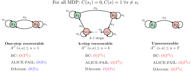
Figure 4: Three different MDPs with varying recoverability regimes. For all MDPs, $C(s_{1})=0$ and $C(s)=1$ for all $s\neq s_{1}$. The expert deterministic policy is therefore $\pi^{*}(s_{1})=a_{1}$ and $\pi^{*}(s)=a_{2}$ for all $s\neq s_{1}$. Even with one-step recoverability, BC can still result in $O(T^{2}\epsilon)$ error. For $>1$-step recoverability, even Fail slides to $O(T^{2}\epsilon)$, while DAgger can recover in $k$ steps leading to $O(kT\epsilon)$. For unrecoverable problem, all algorithms can go upto $O(T^{2}\epsilon)$. Hence recoverability dictates the lower-bound of how well we can do in the model misspecified regime.

Here we show that recoverability, in a weaker sense than Def. 5.1, is a fundamental requirement for any IL algorithm. Consider the class of MDPs defined in Fig. 4. They vary in a weaker sense of recoverability, i.e. the upper bound of the advantage $\left|\left|A^{\pi^{*}}(s,a)\right|\right|_{\infty}\leq u$. The first MDP has $u=1$, allowing for one-step recoverability and hence Fail achieves $O(T\epsilon)$ while BC suffers from compounding error $O(T^{2}\epsilon)$. The second MDP needs atleast $k-$step to recover, thus both BC and ALICE hit $O(T^{2}\epsilon)$, while DAgger can achieve the best bound of $O(kT\epsilon)$. Finally, for unrecoverable MDPs, all algorithms are resigned to $O(T^{2}\epsilon)$.

A.6 IL Baseline Implementation Specifics

We use the following settings in training our RL experts (using the RL Baselines Zoo Python package) and IL learners. Learner policy classes consisted of neural networks with relu activation everywhere except final layer and a set number of hidden dimensions (layer 1 dimension, layer 2 dimension, …). These experiments are all in the stationary setting, where a single policy is trained on all available data and executed for all time-steps.

Box2d Discrete OpenAI Gym	MuJoCo Continuous Control
(CartPole, Acrobot, MountainCar)	(Ant, HalfCheetah, Reacher, Walker, Hopper)
RL Expert	RL Expert
Deep Q Network	Soft Actor Critic
100k env. steps	3M env. steps
exploration fraction = 50%	learning rate = 0.0003
final $\epsilon=0.1$	buffer size = 1M
IL Learner	IL Learner
learning rate = 0.001	learning rate = 0.001
hidden layer dimensions = (64,)	hidden layer dimensions = (512,512)
100k optimization steps	20M optimization steps

Table 2: Settings used for training RL experts and IL learners

In some settings, it is natural and useful to augment the current observation $s_{t}$ with previous action $a_{t-1}$, i.e. $s_{t}=[s_{t},a_{t-1}]$. We refer to this addition of single-step action history to BC as ”BC+H” and include

Environment	Expert	BC	BC+H
CartPole-v1	$500.0\pm 0.0$	$500.0\pm 0.0$	$500.0\pm 0.0$
Acrobot-v1	$-71.7\pm 11.5$	$-78.4\pm 14.2$	$-80.0\pm 18.0$
MountainCar-v0	$-99.6\pm 10.9$	$-107.8\pm 16.4$	$-105.4\pm 16.6$
Ant-v2	$4185.9\pm 1081.1$	$3352.9\pm 1800.9$	$2919.2\pm 1967.9$
HalfCheetah-v2	$4514.6\pm 111.4$	$4388.4\pm 494.8$	$4338.1\pm 791.7$
Reacher-v2	$-4.4\pm 1.3$	$-4.9\pm 2.4$	$-4.5\pm 1.4$
Walker2d	$5496\pm 89$	$5349\pm 634$	$4451\pm 1491$

Table 3: Behavioral Cloning performance on common control benchmarks for 25 expert trajectories. In most cases, BC performs within the expert’s error margin and often as well as more sophisticated methods. See appendix for more results and implementation specifics.

Although we did not perform experiments for the partially observable setting, please refer to the experiments of (Wen et al., 2020). They use a generative adversarial approach to generate an intermediate state representation that removes all information of the previous action. Although their vanilla implementation of BC didn’t achieve the strongest results, they include an implementation of their algorithm without the use of an adversary, effectively performing BC with a more principled autoencoder-type model class. Using that improved model class, they show that BC achieves similar reward to DAgger in many of their experiments. We also refer the reader to (Sun et al., 2019) for experimental results of Loss #2 (Fail) in the non-stationary policy setting.

References

- Abbeel & Ng (2004) Abbeel, P. and Ng, A. Y. Apprenticeship learning via inverse reinforcement learning. In Proceedings of the twenty-first international conference on Machine learning, pp. 1, 2004.
- Bagnell (2016) Bagnell, D. Feedback in machine learning. In Workshop on Safety and control for artificial intelligence, CMU, 2016.
- Bansal et al. (2018) Bansal, M., Krizhevsky, A., and Ogale, A. Chauffeurnet: Learning to drive by imitating the best and synthesizing the worst. arXiv preprint arXiv:1812.03079, 2018.
- Barde et al. (2020) Barde, P., Roy, J., Jeon, W., Pineau, J., Pal, C., and Nowrouzezahrai, D. Adversarial soft advantage fitting: Imitation learning without policy optimization. arXiv preprint arXiv:2006.13258, 2020.
- Beygelzimer et al. (2008) Beygelzimer, A., Langford, J., and Zadrozny, B. Machine learning techniques—reductions between prediction quality metrics. In Performance Modeling and Engineering, pp. 3–28. Springer, 2008.
- Bojarski et al. (2016) Bojarski, M., Del Testa, D., Dworakowski, D., Firner, B., Flepp, B., Goyal, P., Jackel, L. D., Monfort, M., Muller, U., Zhang, J., et al. End to end learning for self-driving cars. arXiv preprint arXiv:1604.07316, 2016.
- Brantley et al. (2019) Brantley, K., Sun, W., and Henaff, M. Disagreement-regularized imitation learning. In International Conference on Learning Representations, 2019.
- Codevilla et al. (2019) Codevilla, F., Santana, E., López, A. M., and Gaidon, A. Exploring the limitations of behavior cloning for autonomous driving. In Proceedings of the IEEE International Conference on Computer Vision, pp. 9329–9338, 2019.
- de Haan et al. (2019) de Haan, P., Jayaraman, D., and Levine, S. Causal confusion in imitation learning. In Advances in Neural Information Processing Systems, pp. 11693–11704, 2019.
- Finn et al. (2016) Finn, C., Levine, S., and Abbeel, P. Guided cost learning: Deep inverse optimal control via policy optimization. In International conference on machine learning, pp. 49–58, 2016.
- Ho & Ermon (2016) Ho, J. and Ermon, S. Generative adversarial imitation learning. In Advances in neural information processing systems, pp. 4565–4573, 2016.
- Kolter & Maloof (2007) Kolter, J. Z. and Maloof, M. A. Dynamic weighted majority: An ensemble method for drifting concepts. Journal of Machine Learning Research, 8(Dec):2755–2790, 2007.
- Kuefler et al. (2017) Kuefler, A., Morton, J., Wheeler, T., and Kochenderfer, M. Imitating driver behavior with generative adversarial networks. In 2017 IEEE Intelligent Vehicles Symposium (IV), pp. 204–211. IEEE, 2017.
- Laskey et al. (2017) Laskey, M., Chuck, C., Lee, J., Mahler, J., Krishnan, S., Jamieson, K., Dragan, A., and Goldberg, K. Comparing human-centric and robot-centric sampling for robot deep learning from demonstrations. In 2017 IEEE International Conference on Robotics and Automation (ICRA), pp. 358–365. IEEE, 2017.
- Muller et al. (2006) Muller, U., Ben, J., Cosatto, E., Flepp, B., and Cun, Y. L. Off-road obstacle avoidance through end-to-end learning. In Advances in neural information processing systems, pp. 739–746, 2006.
- Pearl et al. (2016) Pearl, J., Glymour, M., and Jewell, N. P. Causal inference in statistics: A primer. John Wiley & Sons, 2016.
- Pomerleau (1989) Pomerleau, D. Alvinn: An autonomous land vehicle in a neural network. In Touretzky, D. (ed.), Proceedings of Advances in Neural Information Processing Systems 1, pp. 305 –313. Morgan Kaufmann, December 1989.
- Ross (2013) Ross, S. Interactive learning for sequential decisions and predictions. 2013.
- Ross & Bagnell (2010) Ross, S. and Bagnell, D. Efficient reductions for imitation learning. In Proceedings of the thirteenth international conference on artificial intelligence and statistics, pp. 661–668, 2010.
- Ross et al. (2011) Ross, S., Gordon, G., and Bagnell, J. A. A reduction of imitation learning and structured prediction to no-regret online learning. In AISTATS, 2011.
- Sculley et al. (2014) Sculley, D., Holt, G., Golovin, D., Davydov, E., Phillips, T., Ebner, D., Chaudhary, V., and Young, M. Machine learning: The high interest credit card of technical debt. In SE4ML: Software Engineering for Machine Learning (NIPS 2014 Workshop), 2014.
- Shalev-Shwartz & Kakade (2008) Shalev-Shwartz, S. and Kakade, S. M. Mind the duality gap: Logarithmic regret algorithms for online optimization. Advances in Neural Information Processing Systems, 21:1457–1464, 2008.
- Shimodaira (2000) Shimodaira, H. Improving predictive inference under covariate shift by weighting the log-likelihood function. Journal of statistical planning and inference, 90(2):227–244, 2000.
- Spirtes et al. (2000) Spirtes, P., Glymour, C. N., Scheines, R., and Heckerman, D. Causation, prediction, and search. MIT press, 2000.
- Sun et al. (2019) Sun, W., Vemula, A., Boots, B., and Bagnell, J. A. Provably efficient imitation learning from observation alone. In Proceedings of (ICML) International Conference on Machine Learning, June 2019.
- Wen et al. (2020) Wen, C., Lin, J., Darrell, T., Jayaraman, D., and Gao, Y. Fighting copycat agents inbehavioral cloning from observation histories. In Advances in Neural Information Processing Systems, 2020.
- Zhang et al. (2020) Zhang, J., Kumor, D., and Bareinboim, E. Causal imitation learning with unobserved confounders. In Advances in Neural Information Processing Systems, 2020.
- Ziebart et al. (2008) Ziebart, B. D., Maas, A. L., Bagnell, J. A., and Dey, A. K. Maximum entropy inverse reinforcement learning. In Aaai, volume 8, pp. 1433–1438. Chicago, IL, USA, 2008.
- Zinkevich (2003) Zinkevich, M. Online convex programming and generalized infinitesimal gradient ascent. In Proceedings of the 20th international conference on machine learning (icml-03), pp. 928–936, 2003.