Halo EFT calculation of charge form factor for two-neutron ${}^{6}\textrm{He}$ halo nucleus: two-body resonant P-wave interaction

Abstract

We take a new look at ${}^{6}\textrm{He}$ halo nucleus and set up a halo effective field theory at low energies to calculate the charge form factor of ${}^{6}\textrm{He}$ system with resonant P-wave interaction. P-wave Lagrangian has been introduced and the charge form factor of ${}^{6}\textrm{He}$ halo nucleus has been obtained at Leading-Order. In this study, the mean-square charge radius of ${}^{6}\textrm{He}$ nucleus relative to ${}^{4}\textrm{He}$ core and the root-mean-square (r.m.s) charge radius of ${}^{6}\textrm{He}$ nucleus have been estimated as $\langle r_{E}^{2}\rangle=1.408\;\textrm{fm}^{2}$ and $\langle r_{E}^{2}\rangle_{{}^{6}He}^{\frac{1}{2}}=2.058\;\textrm{fm}$, respectively. We have compared our results with the other available theoretical and experimental data.

1 Introduction

Weinberg was the first one who applied the effective field theory (EFT) to nuclear forces h12 . Also the concept of applying EFT to nuclear forces was brought by Rho h41 and by Ordóñez and van Kolck h42 . An effective field theory includes the appropriate degrees of freedom to describe physical phenomena occurring at a chosen length scale or energy scale. Up to now, cold atoms and few-nucleon systems at low energies have been studied by this formalism h13 ; h14 ; h15 . Pion-exchange effects are not resolved at low energies and momenta ($E<\frac{m_{\pi}^{2}}{M_{N}},\;p\leq m_{\pi}$, where $m_{\pi}$ and ${M_{N}}$ are the mass of pion and nucleon respectively), so this theory is constructed by only short-range contact interactions known as pionless effective field theory $(\textrm{EFT}(\pi\mkern-9.5mu/))$ h16 ; h17 ; h18 .

One of the major challenges for nuclear theory is the calculation of properties of halo nuclei. These nuclei are characterized by a tightly bound core and one or two weakly bound valence nucleons h19 ; h20 ; h21 ; h22 . In halo EFT, either core or nucleons are treated as the fundamental fields and one can find relations between different nuclear low-energy observables in this EFT. On the other hand, most systems can be explained by a short-range EFT expanding in $\frac{R}{a}$, which $R$ is the range of the nucleon-nucleus interaction such that $M_{high}\sim\frac{1}{R}$ and $a$ is the two-body scattering length such that $M_{low}\sim\frac{1}{a}$, so it is found that $R\ll a$. Based on an EFT in terms of the expansion parameter $\frac{R}{|a|}$, 2n halo nuclei are described as an effective three-body system including of a core and two weakly-attached valence neutrons. Some universal properties of these nuclei are investigated such as the matter density form factors and mean square radii h23 ; h24 .

Investigations have been carried out into Borromean nuclei such as ${}^{11}\textrm{Li}$, ${}^{14}\textrm{Be}$ ,and ${}^{6}\textrm{He}$ h19 ; h20 ; h23 ; h24 . While these nuclei have only one bound state, there are no bound states in the binary subsystems. Properties of one neutron halo nucleus ${}^{8}\textrm{Li}$ has been pursued by the two-body sector halo EFT h25 ; h26 ; h46 . A detailed analysis of electromagnetic properties of halo nuclei ${}^{11}\textrm{Be}$ system investigated where the low-energy E1 strength function in breakup to the ${}^{10}\textrm{Be}$-neutron channel has been performed h36 .

The lightest nuclei with 2n-halo structure are ${}^{6}\textrm{He}$, ${}^{11}\textrm{Li}$, ${}^{14}\textrm{Be}$, ${}^{22}\textrm{C}$, and ${}^{17}\textrm{B}$. Hagen et al. h8 and Vanasse h28 have studied the S-wave EFT framework for ${}^{11}\textrm{Li}$, ${}^{14}\textrm{Be}$, and ${}^{22}\textrm{C}$ nuclei and calculated corresponding charge radius. Other two-neutron halo nucleus, ${}^{17}\textrm{B}$, will be dealt with in the future works. The halo EFT we construct includes the two-body P-wave interaction in the $n\alpha$ subsystem of ${}^{6}\textrm{He}$ nucleus. Binding energies, radii and other properties of various halo nuclei of s-wave and p-wave type have been reviewed in halo EFT h44 . Ji $\it etal.$ have considered a halo EFT for the three-body $nn\alpha$ system to explain the ${}^{6}\textrm{He}$ ground state h4 . An EFT with P-wave resonance interactions has been developed for elastic $n\alpha$ scattering by Bertulani et al. h1 . Bedaque $\it etal.$ h43 have suggested a different power counting compared to h1 to describe narrow resonances in EFT and illustrated their results in the case of nucleon-alpha scattering. The electric dipole strength function distribution of the ${}^{6}\textrm{He}$ halo nucleus has been recently evaluated based on the halo EFT approach using the particle-dimer scattering amplitudes in the $nn\alpha$ system and the normalized ${}^{6}\textrm{He}$ wave function h3 . Finally, the momentum-space probability density of ${}^{6}\textrm{He}$ at leading order in halo EFT has been presented. The momentum distribution of ${}^{6}\textrm{He}$ requires the n-n and n-core t-matrices as well as a c-n-n force as input in the Faddeev equations h37 .

In this paper, we focus on the two-neutron halo nucleus ${}^{6}\textrm{He}$, calculate the electric charge form factor and find the root-mean-square (r.m.s) charge radius of ${}^{6}\textrm{He}$ nucleus. Therefore we introduce the strong Lagrangian including $n\alpha$ P-wave interaction for the halo EFT at leading order in Section 2. In Section 3, the formalism for two- and three-body propagators are completely presented. ${}^{6}\textrm{He}$ charge form factor is evaluated in Section 4. In Section 5, our numerical results for the form factor and the charge radius are presented and compared with experimental data. Finally, we conclude in Section 6. In Appendix A, the particle-dimer scattering is explained and in Appendix B, some expressions for the contributions of diagrams participate into the form factor of ${}^{6}\textrm{He}$ are presented in details.

2 Strong interaction

2.1 Power-counting

We apply a halo effective field theory in non-relativistic formalism for the alpha core ($\alpha$) with spin zero interacting with two spin half neutrons. In this method, we define $Q$ as a low momentum scale attributed to core and neutron momentums. Furthermore, the high momentum parameter, $\bar{\Lambda}$ can be scaled as $\bar{\Lambda}\sim m_{\pi}\sim\sqrt{m_{\alpha}E_{\alpha}}$ where $m_{\alpha}$ and $E_{\alpha}=20.21\;\textrm{MeV}$ refer to the mass and the excitation energy of $\alpha$ particle. There are the two-body neutron-neutron ($nn$) and the neutron-alpha ($n\alpha$) interactions in ${}^{6}\textrm{He}$ calculation. The remarkable state in the $nn$ is $S$-wave virtual bound state. A low-momentum scale $Q$ is defined by the inverse of the di-neutron scattering length, $\frac{1}{(a_{0}=-23.714)}\;\textrm{fm}^{-1}$ and the inverse of the effective range of this S-wave state, $\frac{1}{(r_{0}=2.73)}\;\textrm{fm}^{-1}$ is considered as the high-momentum scale $\bar{\Lambda}$. So, the leading order (LO) scattering amplitude of two neutrons is constructed by the scattering length contribution only. With respect to these scales, the $S$-wave effective range expansion (ERE) for di-neutron system at the lowest-order can be given by

$$k\cot\delta_{0}=-\frac{1}{a_{0}}+\cdots.$$ (1)

In low-energy region, only $S$- and $P$-wave interactions are significant in the $n\alpha$ system. There are three possible partial waves for the $n\alpha$ system, ${}^{2}S_{1/2}$, ${}^{2}P_{1/2}$ and ${}^{2}P_{3/2}$. We use the power counting introduced by Bertulani et al. in Ref. h1 which also applied in the Gamow shell model calculation of ${}^{6}\textrm{He}$ in halo EFT h5 . This power counting specifies that $n\alpha$ interaction gets the LO contributions only from both scattering length and effective range of ${}^{2}P_{3/2}$ channel as

$$\frac{1}{a_{1}}\sim Q^{3}\;\;,\;\;\frac{r_{1}}{2}\sim Q\;\;,\;\;\frac{\mathcal{P}_{1}}{4}\sim\frac{1}{\bar{\Lambda}},$$ (2)

where $a_{1}=-62.95\;\textrm{fm}^{3}$, $r_{1}=-0.88\;\textrm{fm}^{-1}$ and $\mathcal{P}_{1}=-3.0\;\textrm{fm}$ are the scattering length, the effective range and the shape parameter of ${}^{2}P_{3/2}$ state, respectively h2 . Therefore the lowest-order terms of effective range expansion for the resonant P-wave $n\alpha$ system are given by

$$k^{3}\cot\delta_{1}=-\frac{1}{a_{1}}+\frac{r_{1}}{2}k^{2}+\cdots.$$ (3)

2.2 Lagrangians

Generally, the effective field theory expansion parameter is defined by the momentum ratio $Q/\bar{\Lambda}$ and it creates the order-by-order pattern of convergence. At LO, the Lagrangian for ${}^{6}\textrm{He}$ system can be written as the summation of one-, two- and three-body contributions, $\mathcal{L}=\mathcal{L}^{(1)}+\mathcal{L}^{(2)}+\mathcal{L}^{(3)}$ , where

$$\mathcal{L}^{(1)} = n^{{\dagger}}\Big{(}i\partial_{0}+\frac{\vec{\nabla}^{2}}{2m_{n}}\Big{)}n+\phi^{{\dagger}}\Big{(}i\partial_{0}+\frac{\vec{\nabla}^{2}}{2m_{\alpha}}\Big{)}\phi$$

$$\mathcal{L}^{(2)} = \Delta_{0}d_{0}^{{\dagger}}d_{0}-\frac{g_{0}}{\sqrt{8}}\Big{(}d_{0}^{{\dagger}}(n^{{\dagger}}i\sigma_{2}n)+h.c.\Big{)}$$

$$+ \eta_{1}d^{{\dagger}}_{1}\Big{[}i\partial_{0}+\frac{\vec{\nabla}^{2}}{2(m_{n}+m_{\alpha})}-\Delta_{1}\Big{]}d_{1}$$

$$+ \frac{g_{1}}{2}\Big{[}d^{{\dagger}}_{1}\vec{S}^{{\dagger}}\cdot[n\vec{\nabla}\phi-(\vec{\nabla}n)\phi]+h.c.$$

$$- r[d^{{\dagger}}_{1}\vec{S}^{{\dagger}}\cdot{\vec{\nabla}(n\phi)}+h.c.]\Big{]}$$

$$\mathcal{L}^{(3)} = \Omega t^{{\dagger}}t-h\frac{\sqrt{3m_{n}}g_{1}}{2\Lambda}\Big{[}t^{{\dagger}}(d_{1}(i\sigma_{2})\vec{S}\cdot\vec{P}n)+h.c.\Big{]},$$ (4)

where $m_{n}$ is the neutron mass and $n,\phi,d_{0}\;(d_{1})$ denote the two component spinor field of the neutron, the bosonic alpha core field, the auxiliary dimer field of $nn$ ($n\alpha$) system. Also, $t$ implies a spin-0 trimer auxiliary field. Moreover we have

$$\vec{P}=\frac{\tilde{\mu}}{\overrightarrow{m}}i\overleftarrow{\nabla}-\frac{\tilde{\mu}}{\overleftarrow{m}}i\overrightarrow{\nabla},$$ (5)

that $\overrightarrow{m}$ ($\overleftarrow{m}$)implies the mass of $n\;(d_{1})$ field and $\tilde{\mu}$ denotes the reduced mass of $n-d_{1}$ system. $\eta_{1}$ is equal to $\pm 1$ , $g_{0}^{2}=\frac{4\pi}{m_{n}}$ and $r=\frac{(m_{\alpha}-m_{n})}{(m_{\alpha}+m_{n})}$. Also, $\sigma_{2}$ indicates the Pauli matrix so that the spin projection matrix ($\frac{i}{\sqrt{2}}\sigma_{2}$) projects the two neutrons on the spin-singlet case. In Eq. (4), the $S_{i}$${}^{,}s$ are the 2$\times$4 matrices connecting states with total angular momentum $j=1/2$ and $j=3/2$. These matrices satisfy the following relations

$$S_{i}S^{{\dagger}}_{j} = \frac{2}{3}\delta_{ij}-\frac{i}{3}\epsilon_{ijk}\sigma_{k},$$

$$S^{{\dagger}}_{j}S_{i} = \frac{3}{4}\delta_{ij}-\frac{1}{6}\{J_{i}^{3/2},J_{j}^{3/2}\}+\frac{i}{3}\epsilon_{ijk}J_{k}^{3/2},$$ (6)

where $J_{i}^{3/2}$ are the generators of the $J=3/2$ representation of the rotation group. The parameter $\Delta_{0}$ should be fixed from matching the pionless EFT $nn$ scattering amplitude to the ERE scattering amplitude of two non-relativistic nucleons. Also we have the following relations h1

$$g_{1}^{2}=-\eta_{1}\frac{6\pi}{\mu^{2}r_{1}}\;\;,\;\;\Delta_{1}=\frac{1}{\mu a_{1}r_{1}},$$ (7)

where $\mu$ is the reduced mass of $n\alpha$ system. According to the sign of $r_{1}$ the sign $\eta_{1}$ should be fixed to +1. Due to gauge invariance of the non-interacting parts of Lagrangian for charged alpha and $d_{1}$-dimer, we include electromagnetic coupling with vector potential $A_{\mu}$. This minimal coupling gives the covariant derivative as

$$\partial_{\mu}\rightarrow D_{\mu}=\partial_{\mu}+i\hat{Q}A_{\mu},$$ (8)

that $A_{\mu}$ satisfies the Coulomb gauge fixing relation as $\vec{\nabla}$ $\!\!\cdot\vec{A}=0$. In Eq. (8), $\hat{Q}$ introduces the charge operator such that $\hat{Q}\phi=\mathcal{Z}e\phi$, $\hat{Q}d_{1}=\mathcal{Z}ed_{1}$, $\hat{Q}n=0$, and $\hat{Q}d_{0}=0$, where $\mathcal{Z}$ is the number of protons in the alpha core.

3 Two-body and three-body systems

3.1 Two body propagator

The full dimer propagators are obtained by the infinite sum of diagrams shown in Fig. 1. The solid lines indicate neutron and the dashed lines are the $\alpha$ particle. The bare $nn$-dimer propagator has been depicted by double solid lines with empty arrow, and the bare $n\alpha$-dimer propagator is observed by dashed-solid lines with empty arrow.

Based on introduced power counting, the LO full dimer propagators shown by filled arrow in Fig. (1) for auxiliary field $d_{0}$ and $d_{1}$ are obtained by the following expressions

$$iD_{0}(p_{0},\textbf{p})=\frac{i}{\frac{1}{a_{0}}-\sqrt{\frac{\textbf{p}^{2}}{4}-m_{n}p_{0}-i\epsilon}},$$

$$iD_{1}(p_{0},\textbf{p})_{\bar{\alpha}}^{\bar{\beta}}=i\eta_{1}\delta_{\bar{\alpha}}^{\bar{\beta}}\bigg{\{}p_{0}-\frac{\textbf{p}^{2}}{2(m_{n}+m_{\alpha})}-\frac{1}{\mu a_{1}r_{1}}$$

$$\quad-\frac{1}{\mu r_{1}}\big{(}\frac{\mu}{m_{n}+m_{\alpha}}\textbf{p}^{2}-2\mu p_{0}-i\epsilon\big{)}^{\frac{3}{2}}+i\epsilon\bigg{\}}^{-1},$$

(9)

that the incoming and outgoing spin components of $d_{1}$-dimer is indicated by $\bar{\alpha}$ and $\bar{\beta}$ respectively. Because of $J=\frac{3}{2}$ of $d_{1}$-dimer, $\delta_{\bar{\alpha}}^{\bar{\beta}}$ is a $4\times 4$ unit matrix.

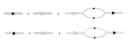
Figure 1: Dressing the bare $nn\;(n\alpha)$ dimer propagator with bubble diagrams leads to the full $nn\;(n\alpha)$ dimer propagator to all orders. The solid lines show neutron and the dashed lines are the $\alpha$ particle. Double solid lines with empty (filled) arrow are the bare (full) $d_{0}$-dimer propagators and dashed-solid lines with empty (filled) arrow are the bare (full) $d_{1}$-dimer propagators.

3.2 Three point function

3.2.1 Full trimer propagator

The amplitude of the particle-dimer scattering process in $nn\alpha$ system has been calculated using the Faddeev equation introduced in Appendix A. The transition amplitude (T-matrix) has a pole at three-body bound state, so the T-matrix can be factorized at energy $E=-B_{2n}$ as h8

$$T(E,k,p)=-\frac{\vec{\mathcal{B}}^{{\dagger}}(k)\;\vec{\mathcal{B}}(p)}{E+B_{2n}}\;+\;\mathrm{regular\;terms},$$ (10)

where $B_{2n}=0.97\;\textrm{MeV}$ h6 denotes the 2n separation energy of system. $\vec{\mathcal{B}}(p)={\mathcal{B}_{0}(p)\choose\mathcal{B}_{1}(p)}$ is the bound state vector, such that ${\mathcal{B}}_{0}\;({\mathcal{B}}_{1})$ corresponds to the $\phi d_{0}\rightarrow\phi d_{0}\;(\phi d_{0}\rightarrow nd_{1})$ transition of the bound state equation according to Eqs. (A.18) and (A.21). Fig. 2 indicates the Feynman diagrams contributing to the full trimer propagator $t(E)$. Based on the three-body interaction introduced in Eq. (A.17), the three-body force appears only between the incoming and outgoing $n+d_{1}$ channels. So, only $T_{11}$ component derived from $2\times 2$ T-matrix integral equation in Eq. (A.5) contributes to $t(E)$. Using Feynman rules and taking into account the projection operator in Eq. (A.4), for a trimer propagator we can write

$$it(E) = \frac{i}{\Omega}\Big{[}1+\frac{m_{n}\;g_{1}^{2}}{\Lambda^{2}}\frac{h^{2}}{\Omega}\int_{0}^{\Lambda}dq\;\frac{q^{2}}{2\pi^{2}}\;q^{2}\;\overline{D}_{1}(E,q)$$ (11)

$$- \frac{m_{n}\;g_{1}^{2}}{6\Lambda^{2}}\frac{h^{2}}{\Omega}\int_{0}^{\Lambda}dq\;\frac{q^{2}}{2\pi^{2}}\;\int_{0}^{\Lambda}dq^{\prime}\;\frac{q^{\prime 2}}{2\pi^{2}}$$

$$\Big{(}\overline{D}_{1}(E,q^{\prime})\;q^{\prime}q\;T_{11}(E,q^{\prime},q)\;\overline{D}_{1}(E,q)\Big{)}\Big{]},$$

where the energy integrals have been carried out and $\overline{D}_{1}(E,q)=D_{1}(E-\frac{q^{2}}{2m_{n}},q)$.

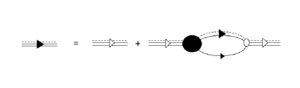
Figure 2: Feynman diagrams for the full trimer propagator $t$. Single, double, triple lines denote neutron, $d_{1}$-dimer and trimer respectively. Triple line with empty (filled) arrow is the bare (full) trimer propagator.

3.2.2 Trimer wave function renormalization

The trimer wave function renormalization constant can be extracted from the following relation h8 ; h39

$$Z_{t}=\lim_{E\to-E^{(3)}}(E+E^{(3)})\;t(E),$$ (12)

where $E^{(3)}=B_{2n}$. By neglecting the regular functions in terms of $E$ corresponding to the first and second terms in Eq. (11), we substitute the last term of $t(E)$ into Eq. (12) and finally obtain

$$Z_{t} = \frac{m_{n}\;g_{1}^{2}}{6\Lambda^{2}}\frac{h^{2}}{\Omega^{2}}$$ (13)

$$\lim_{E\to-E^{(3)}}\Big{[}-(E+E^{(3)})\int_{0}^{\Lambda}dq\;\frac{q^{3}}{2\pi^{2}}\;\int_{0}^{\Lambda}dq^{\prime}\;\frac{q^{\prime 3}}{2\pi^{2}}$$

$$\times\Big{(}\overline{D}_{1}(E,q^{\prime})\;T_{11}(E,q^{\prime},q)\;\overline{D}_{1}(E,q)\Big{)}\Big{]}.$$

For the incoming and outgoing $n+d_{1}$ channels, inserting Eq. (10) into Eq. (13) yields

$$Z_{t} = \frac{m_{n}\;g_{1}^{2}}{6\Lambda^{2}}\frac{h^{2}}{\Omega^{2}}\int_{0}^{\Lambda}dq\;\frac{q^{3}}{2\pi^{2}}\;\int_{0}^{\Lambda}dq^{\prime}\;\frac{q^{\prime 3}}{2\pi^{2}}$$ (14)

$$\times\Big{(}\overline{D}_{1}(-B_{2n},q^{\prime})\;{\mathcal{B}}^{{\dagger}}_{1}(q^{\prime})\;{\mathcal{B}}_{1}(q)\;\overline{D}_{1}(-B_{2n},q)\Big{)}$$

$$= \frac{m_{n}\;g_{1}^{2}}{6\Lambda^{2}}\frac{h^{2}}{\Omega^{2}}\;\left|\int_{0}^{\Lambda}dq\frac{q^{3}}{2\pi^{2}}\overline{D}_{1}(-B_{2n},q){\mathcal{B}}_{1}(q)\right|^{2}.$$

3.2.3 Trimer-dimer-particle three point function $\vec{\mathcal{G}}^{irr}$

The calculation of the charge form factor of ${}^{6}\textrm{He}$ halo nucleus requires the trimer-dimer-particle three point function $\vec{\mathcal{G}}^{irr}$. The LO $\vec{\mathcal{G}}^{irr}$ function is illustrated by the coupled integral equation in Fig. 3.

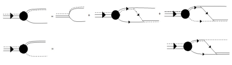
Figure 3: Diagrammatic representation of coupled integral equation for the trimer-dimer-particle three point function $\vec{\mathcal{G}}^{irr}$.

$\vec{\mathcal{G}}^{irr}$ is a vector with two components as $\vec{\mathcal{G}}^{irr}(E,p)={\mathcal{G}^{irr}_{0}\choose\mathcal{G}^{irr}_{1}}$, where $\mathcal{G}^{irr}_{0}$ $(\mathcal{G}^{irr}_{1})$ is the three point function for trimer constructed by $\alpha-d_{0}$ ($n-d_{1}$) system. Using introduced Lagrangian in Eq. (4) and Feynman rules, we can obtain the relation for two components of $\vec{\mathcal{G}}^{irr}$ as

$$i\;\mathcal{G}_{i}^{irr}(E,k)=i\frac{\sqrt{m_{n}}}{\Lambda}\;g_{1}\;h\;\frac{\sqrt{3}}{2}\Big{[}\delta_{1i}\;\vec{S^{{\dagger}}}\cdot\vec{k}\;\sigma_{2}$$

$$-\int_{0}^{\Lambda}dq\;\frac{q^{2}}{2\pi^{2}}\;\Big{(}\vec{S^{{\dagger}}}\cdot\vec{q}\;\sigma_{2}\Big{)}\left.\overline{D}_{1}(E,q)\;T_{1i}(E,q,k)\right|_{H=0}\Big{]},$$

(15)

where the three-body force $H$ has been introduced in Eq. (A.17). All trimer-reducible contributions are neglected by setting $H=0$ in Eq. (15) h8 . Taking into consideration $\left.T_{1i}(E,q,k)\right|_{H=0}$ component of Eq. (A.5), we have

$$\mathcal{G}_{i}^{irr}(E,k)=\frac{\sqrt{m_{n}}}{\Lambda}\;g_{1}\;h\;\frac{\sqrt{3}}{2}\delta_{1i}\;\vec{S^{{\dagger}}}\cdot\vec{k}\;\sigma_{2}$$

$$-\sum_{j=0}^{1}\int_{0}^{\Lambda}dq\frac{q^{2}}{2\pi^{2}}\mathcal{G}_{j}^{irr}(E,q)\overline{D}_{j}(E,q)\;R_{ji}(E,q,k),$$ (16)

where $i,j=0,1$ denote the components of kernel matrix corresponding to $R_{00}$, $R_{01}$, $R_{10}$, and $R_{11}$ that have been derived in Eqs. (A.9)-(A.12). Taking into account the projection operator based on Eq. (A.4), we have

$$\textrm{Tr}\Big{(}\sqrt{\frac{3}{2}}\;\sigma_{2}\;(\hat{e_{k}}\cdot\vec{S})\;\vec{S^{{\dagger}}}\cdot\vec{k}\;\sigma_{2}\Big{)}=\sqrt{\frac{8}{3}}\;k,$$ (17)

therefore, the matrix integral equation for the P-wave irreducible trimer-dimer-particle three point function is given by

$$\vec{\mathcal{G}}^{irr}(E,k) = Z_{t}^{\frac{1}{2}}\frac{\sqrt{m_{n}}}{\Lambda}\;g_{1}\;h\;\sqrt{2}\;k\;\hat{\upsilon}$$

$$- \int_{0}^{\Lambda}dq\;\frac{q^{2}}{2\pi^{2}}\;\Big{(}R(E,q,k)\;D(E,q)\;\vec{\mathcal{G}}^{irr}(E,q)\Big{)},$$

where $2\times 2$ kernel matrix $R$ has been defined in Eq. (A.9) and we have

$$D(E,q)\equiv\left(\begin{array}[]{cc}\overline{D}_{0}(E,q)&0\\ 0&\overline{D}_{1}(E,q)\\ \end{array}\right),$$ (21)

with $\overline{D}_{0}(E,q)=D_{0}(E-\frac{q^{2}}{2m_{\alpha}},q)$ and $\overline{D}_{1}(E,q)=D_{1}(E-\frac{q^{2}}{2m_{n}},q)$.

Two components of Eq. (LABEL:e32) that enter into the calculation of form factor for the ${}^{6}\textrm{He}$ halo nucleus are derived as

$$\mathcal{G}_{i}^{irr}(E,k) = \frac{1}{\sqrt{3}}\;\frac{m_{n}\;g_{1}^{2}}{\Lambda^{2}}\;\left|\beta\;H_{0}(\Lambda)\right|\Big{[}k\;\delta_{1i}$$

$$- \int_{0}^{\Lambda}dq\;\frac{q^{2}}{2\pi^{2}}\;\Big{(}q\;\left.\overline{D}_{1}(E,q)\;T_{1i}(E,q,k)\right|_{H=0}\Big{)}\Big{]},$$

where

$$\beta=\int_{0}^{\Lambda}dq\;\frac{q^{2}}{2\pi^{2}}\;q\;\overline{D}_{1}(-B_{2n},q)\;{\mathcal{B}}_{1}(q),$$ (23)

and the calculation of $H_{0}(\Lambda)=\frac{h^{2}}{\Omega}$ requires the normalized ${}^{6}\textrm{He}$ wave function which is obtained by solving the bound state equation corresponding to the homogeneous part of Eq. (A.5) with $E=-B_{2n}$. We should mention that $(\hat{\upsilon})_{i}=\delta_{1i}$ and after multiplying $\sqrt{Z_{t}}$ in Eq. (LABEL:e32) $\vec{\mathcal{G}}^{irr}$ has the cutoff dependence which is small enough to render our predictions renormalized.

4 Charge form factor of ${}^{6}\textrm{He}$ halo nucleus

We present a formalism for form factor calculation of ${}^{6}\textrm{He}$ halo nucleus with shallow P-wave interaction. We initially emphasize that all calculations have been performed in the Breit frame in which no energy is carried by the photon. This implies $P_{0}=K_{0}$ and $\vec{P}^{2}=\vec{K}^{2}$ where $\vec{P}$ $(\vec{K})$ denotes the incoming (outgoing) three momentum of trimer. The ${}^{6}\textrm{He}$ charge form factor only depends on the three-momentum of the photon $\vec{Q}^{2}=(\vec{K}-\vec{P})^{2}$ according to h9 ; h40

$$\langle t(K_{0},\vec{K})|j_{0}|t(P_{0},\vec{P})\rangle=(-ie\mathcal{Z})\mathcal{F}_{E}(\vec{Q}^{2})=Z_{t}i\Gamma(\vec{Q}),$$

(24)

where $\mathcal{Z}$ implies the atomic number of ${}^{4}\textrm{He}$ nucleus and $j_{0}$ is the zeroth component of the electromagnetic current.

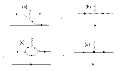
Figure 4: Diagrammatic representation of the matrix element $\overline{\Gamma}(\vec{Q})$ in Eq. (25) falling into four different classes (a), (b), (c) and (d). The wavy lines show minimally photon coupled and the vertex depicted by filled circle in diagram (d) indicates minimally coupled photon to the P-wave $d_{1}$-dimer.

At LO, $\Gamma(\vec{Q})$ in Eq. (24) introduces the sum of all diagrams with external trimer lines and minimally coupled photon to the alpha and $d_{1}$-dimer as shown in Fig. 5, so we have

$$i\Gamma(\vec{Q}) = \int\;\frac{d^{4}p}{(2\pi)^{4}}\int\;\frac{d^{4}k}{(2\pi)^{4}}$$ (25)

$$\times i\vec{\mathcal{G}}^{irr}(E,\vec{P},p_{0},\vec{p})^{T}\;i\overline{\Gamma}(E,\vec{P},p_{0},\vec{p},\vec{K},k_{0},\vec{k})\;$$

$$\times i\vec{\mathcal{G}}^{irr}(E,\vec{K},k_{0},\vec{k}).$$

The matrix element $\overline{\Gamma}$ in Eq. (25) is defined by the sum of diagrams that are depicted in Fig. 4. The energy quantity is defined by $E=P_{0}-\frac{\vec{P}^{2}}{2M_{tot}}$, where the kinetic energy of the ${}^{6}\textrm{He}$ system is subtracted and $M_{tot}=m_{\alpha}+2m_{n}$. Therefore, the ${}^{6}\textrm{He}$ charge form factor at LO is found by the sum of diagrams in Fig. 4 as $\mathcal{F}_{E}=\mathcal{F}_{E}^{(a)}+\mathcal{F}_{E}^{(b)}+\mathcal{F}_{E}^{(c)}+\mathcal{F}_{E}^{(d)}$. The wavy lines show minimally coupled photon and the vertex depicted by filled circle in diagram (d) indicates minimally coupled photon to the P-wave $d_{1}$-dimer.
For calculating of the charge form factor, it is necessary to define the relation between $\mathcal{G}_{i}^{irr}(E,\vec{P},p_{0},\vec{p})$ and center-of-mass $(c.m.)$ quantity $\mathcal{G}_{i}^{irr}(E,p)$ from Eq. (LABEL:e33) via the following integral equation

$$\mathcal{G}_{i}^{irr}(E,\vec{P},p_{0},\vec{p})=\frac{1}{\sqrt{3}}\;\frac{m_{n}\;g_{1}^{2}}{\Lambda^{2}}\;\left|\beta\;H_{0}(\Lambda)\right|p\;\delta_{1i}$$

$$- \;\sum_{j=0}^{1}\int_{0}^{\Lambda}dq\frac{q^{2}}{2\pi^{2}}\;R_{ij}\Big{(}\frac{M_{i}}{M_{tot}}E+p_{0}-\frac{\vec{P}\cdot\vec{p}}{M_{tot}}+\frac{p^{2}}{2m_{i}},p,q\Big{)}$$

$$\qquad\times\overline{D}_{j}(E,q)\;\mathcal{G}_{j}^{irr}(E,q),$$

where $m_{i}=m_{n},m_{\alpha}$ for $i=0,1$, respectively, and

$$M_{0}=2m_{n},\;\;\;M_{1}=m_{\alpha}+m_{n}.$$ (27)

After performing calculations according to Eq. (4) and using Feynman rules, we obtain the following final relations for charge form factor contributions of diagrams (a), (b), (c) and (d) in Fig. 5

$$\mathcal{F}^{(a)}(Q^{2}) = \int_{0}^{\Lambda}\frac{p^{2}}{2\pi^{2}}\;dp\;\int_{0}^{\Lambda}\frac{k^{2}}{2\pi^{2}}\;dk\;\vec{\mathcal{G}}^{irr}(p)^{T}$$ (28)

$$\times D(p)\;\Upsilon^{(a)}(Q,p,k)D(k)\;\vec{\mathcal{G}}^{irr}(k),$$

$$\mathcal{F}^{(b)}(Q^{2}) = \;\int_{0}^{\Lambda}\Big{(}-\frac{p^{2}}{2\pi^{2}}\Big{)}\;dp\;\int_{0}^{\Lambda}\Big{(}-\frac{k^{2}}{2\pi^{2}}\Big{)}\;dk$$

$$\times \vec{\mathcal{G}}^{irr}(p)^{T}\;D(p)\;\Upsilon^{(b)}(Q,p,k)\;D(k)\;\vec{\mathcal{G}}^{irr}(k),$$

$$\mathcal{F}^{(c)}(Q^{2})=\;\int_{0}^{\Lambda}\Big{(}-\frac{p^{2}}{2\pi^{2}}\Big{)}\;dp\;\int_{0}^{\Lambda}\Big{(}-\frac{k^{2}}{2\pi^{2}}\Big{)}\;dk\;\vec{\mathcal{G}}^{irr}(p)^{T}$$

$$\times D(p)\;\Upsilon^{(c)}(Q,p,k)\;D(k)\;\vec{\mathcal{G}}^{irr}(k)$$

$$+2\int_{0}^{\Lambda}\Big{(}-\frac{p^{2}}{2\pi^{2}}\Big{)}dp\vec{\mathcal{G}}^{irr}(p)^{T}D(p)\vec{\Upsilon}^{(c)}(Q,p)+\Upsilon^{(c)}_{0}(Q),$$

(30)

and

$$\mathcal{F}^{(d)}(Q^{2}) = \;\int_{0}^{\Lambda}\Big{(}-\frac{p^{2}}{2\pi^{2}}\Big{)}\;dp\;\int_{0}^{\Lambda}\Big{(}-\frac{k^{2}}{2\pi^{2}}\Big{)}\;dk$$ (31)

$$\quad\times\vec{\mathcal{G}}^{irr}(p)^{T}\;D(p)\;\Upsilon^{(d)}(Q,p,k)\;D(k)\;\vec{\mathcal{G}}^{irr}(k)$$

$$+2\int_{0}^{\Lambda}\Big{(}-\frac{p^{2}}{2\pi^{2}}\Big{)}\;dp\;\vec{\mathcal{G}}^{irr}(p)^{T}\;D(p)\;\vec{\Upsilon}^{(d)}(Q,p)$$

$$+\Upsilon^{(d)}_{0}(Q).$$

The detailed derivations of Eqs. (28)-(31) including the definitions of the used functions have been explained in Appendix B.

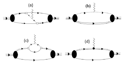
Figure 5: Diagrams for the charge form factor of the ${}^{6}\textrm{He}$ nucleus at LO corresponding to $\mathcal{F}_{E}(\vec{Q}^{2})$ in Eq.(24). Notations are as in Fig. (4).

5 Numerical calculation and results

As we know at $Q^{2}=0$, the charge form factor is normalized to one because of conservation of current. The expansion of the form factor in powers of $Q^{2}$ leads to

$$\mathcal{F}_{E}(Q^{2})=\;1-\;\frac{\langle r_{E}^{2}\rangle}{6}\;Q^{2}+\cdots,$$ (32)

where $\langle r_{E}^{2}\rangle$ is the mean-square charge radius of the ${}^{6}\textrm{He}$ halo system relative to ${}^{4}\textrm{He}$ mean-square charge radius. By taking the limit $Q^{2}\rightarrow 0^{+}$, $\langle r_{E}^{2}\rangle$ can be extracted as

$$\langle r_{E}^{2}\rangle=\;-6\lim_{Q^{2}\to 0^{+}}\frac{d\mathcal{F}_{E}}{dQ^{2}},$$ (33)

and we can obtain the mean-square charge radius of ${}^{6}\textrm{He}$ halo nucleus by the following relation

$$\langle r_{E}^{2}\rangle_{{}^{6}He}=\langle r_{E}^{2}\rangle\;+\langle r_{E}^{2}\rangle_{{}^{4}He}.$$ (34)

It is necessary to point out that we have neglected the small negative mean-square charge radius of the neutron $\langle r_{E}^{2}\rangle_{n}=-0.115\;\textrm{fm}^{2}$ h10 in our calculation. In this section, we apply our P-wave halo EFT formalism to calculate the form factor and the mean-square charge radius of ${}^{6}\textrm{He}$ nucleus relative to ${}^{4}\textrm{He}$ core $(\langle r_{E}^{2}\rangle)$ according to Eq. (33). We compare our EFT evaluation with other available theoretical results. Our formalism applies directly to two-neutron halo nucleus, ${}^{6}\textrm{He}$ with $J^{P}=0^{+}$.

Fitting the three-body binding energy of ${}^{6}\textrm{He}$ nucleus to $B_{2n}=0.97\;\textrm{MeV}$, the three-body force can be determined at leading order. Using this determined three-body force h3 , the renormalized ${}^{6}\textrm{He}$ wave function and so the renormalized trimer-dimer-particle three point function is obtained. The effects of the cutoff dependence for the two components of $\vec{\mathcal{G}}$ function are shown in Fig.6. The plots represent the cutoff variations of the P-wave irreducible trimer-dimer-particle three point function between $\Lambda=600$ MeV and $\Lambda=1200$ MeV with the three-body force which is introduced by Eq. (A.17). As depicted in Fig.6, by considering the three-body force, the cutoff variations of the results are acceptable in comparison with the LO systematical uncertainty. Therefore our numerical results for the trimer-dimer-particle three point function are properly renormalized.

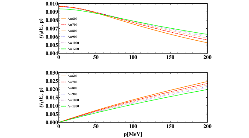
Figure 6: (color online) Two components of the trimer-dimer-particle three point function for the different cutoff values from 600 MeV to 1200 MeV.

As mentioned in Section 2.1, we concentrate on the power counting which is suggested by Bertulani and collaborators in Ref. h1 for the $n\alpha$ interaction. Investigation of the full propagator of the $d_{1}$ field in this power counting discloses in addition to the physical resonance (shallow na resonance), there also exists one spurious pole (the unphysical ${}^{5}\textrm{He}$ bound state) around $p\sim 99$ MeV with negative residue and a deeper binding energy. Using this power counting, the Gamow shell model calculation of ${}^{6}\textrm{He}$ in Ref. h5 removed the spurious pole in the $n\alpha$ T-matrix by constructing bi-orthogonal complete basis.

Table 1: The mean-square charge radius of ${}^{6}\textrm{He}$ nucleus relative to ${}^{4}\textrm{He}$ from Eq. (33) and the r.m.s charge radius of ${}^{6}\textrm{He}$ nucleus according to Eq. (34) that have been compared to the other theoretical and experimental results.

	This	Experimental	Theoretical
	work	Results	Results
$\langle r_{E}^{2}\rangle[\textrm{fm}^{2}]$	1.408	$1.418\pm 0.058$ h31	1.426(38) h35
		$1.047\pm 0.034$ h32
		2.060(8) h33	2.06(1) h35
$\langle r_{E}^{2}\rangle_{{}^{6}He}^{\frac{1}{2}}[\textrm{fm}]$	$2.058$	$2.054\pm 0.014$ h31	2.12(1) h35
			2.147 h29
			2.586 h34

Table 2: The mean-square charge radius of ${}^{6}\textrm{He}$ nucleus relative to ${}^{4}\textrm{He}$ from Eq. (33) and the r.m.s charge radius of ${}^{6}\textrm{He}$ nucleus according to Eq. (34) for different cutoff values.

$\Lambda$ (MeV)	600	700	800	900	1000	1200
$\langle r_{E}^{2}\rangle[\textrm{fm}^{2}]$	1.40822	1.40807	1.40739	1.40786	1.40801	1.40777
$\quad\langle r_{E}^{2}\rangle_{{}^{6}He}^{\frac{1}{2}}[\textrm{fm}]\quad$	2.05766	2.05763	2.05746	2.05758	2.05761	2.05755

In the Halo EFT analysis of the ${}^{6}\textrm{He}$ system, in order to get rid of this spurious pole, one can also treat the unitarity term $ik^{3}$ in the denominator of $n\alpha$ propagator as a perturbation. This method was recently applied to ${}^{6}\textrm{He}$ in Ref. h4 ; Ryberg . One of fundamental drawbacks of this method is that unitarity is lost at LO, which is actually a requirement for the form $\frac{1}{p\cot\delta_{l}-ip}$ that was chosen for the scattering amplitude. In fact the loss of unitarity at LO is not problematic in Ref. h4 , since only bound state observable is considered in the related bound-state three-body calculation. In the Faddeev equation, the resonance pole of $n\alpha$ scattering, which requires the unitary term, was never crossed. However, the unitary term matters if one wants to calculate a resonance state in ${}^{6}\textrm{He}$.

Generally, in the three-body sector, for solving Faddeev integral equation, analogous to the Skornyakov-Ter-Martyrosian (STM) equation for S-wave contact interactions, one can solve Faddeev integral equation for resonant P-wave interactions. In order to discard spurious pole one can use the contour deformation suggested by Hetherington and Schick, namely a rotation $p\rightarrow pe^{-i\Phi}$ ($\Phi>0$) as applied in Ref. h3 for the positive energies.

In this paper we are concerned with the homogeneous part of the integral equations projected onto the bound 0+ ground state of ${}^{6}\textrm{He}$. The position of spurious bound state of a P-wave propagator is on the real axes but for the negative energies $E=E_{B}=-B_{2n}$, Eq. (A.18). One can handle this unphysical deep bound state with similar $p\rightarrow pe^{-i\Phi}$ ($\Phi>0$) analytical continuation by contour rotation of the real axes. In this simpler contour path integral, there is no logarithmic singularities in the loop momentum in comparison with logarithmic singularities in the Legendre functions of second kind in the positive energies on the real axes.

In Fig. 7, our calculation for the charge form factor of ${}^{6}\textrm{He}$ with $\Lambda=700$ MeV is depicted as a function of the photon momentum $(\vec{Q}=\vec{K}-\vec{P})$ in halo EFT. Our results have been compared with distorted wave Born approximation (DWBA) h29 large scale shell model (LSSM) calculations. This model-dependent approach studies ${}^{6}\textrm{He}$ nucleus as a six-body system (not three-body halo one) by using a Woods-Saxon single-particle wave function basis. The difference in the calculated form factors appears as the $Q$ is increasing. As we expect EFT is a model-independent and precision-controlled approach, so including the higher-order corrections can give us better judgment in comparing our three-particle halo formalism with the full six-body DWBA results.

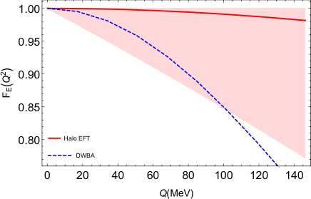
Figure 7: (color online) The charge form factor of the ${}^{6}\textrm{He}$ nucleus with $\Lambda=700$ MeV at LO corresponding to $\mathcal{F}_{E}(\vec{Q}^{2})$ in Eq. (24). The shaded region implies a criterion of estimated theoretical artifacts.

Using Eq. (33), we fit our data for form factor via the standard interpolation method and take the second order derivatives of the fitted function with respect to Q in the limit $Q^{2}\rightarrow 0^{+}$ to evaluate the mean-square charge radius of ${}^{6}\textrm{He}$ nucleus relative to ${}^{4}\textrm{He}$ core. Ingo Sick has studied the world data on elastic electron-Helium scattering to determine a precise value for ${}^{4}\textrm{He}$ r.m.s charge radius and has obtained the value $(1.681\pm 0.004)\;\textrm{fm}$ h30 . In Table 1, we have summarized our EFT evaluated values for the mean-square charge radius of ${}^{6}\textrm{He}$ nucleus relative to ${}^{4}\textrm{He}$ from Eq. (33) and the r.m.s charge radius of ${}^{6}\textrm{He}$ nucleus in comparison with other theoretical and experimental results.

As discussed in the introduction, the expansion parameter of our theory $R_{core}/R_{halo}$ is roughly $R/a$. In order to obtain better estimates, we compare the typical energy scales $E_{halo}$ and $E_{core}$ of the two-neutron halo and the core, respectively. To estimate $E_{halo}$, we choose the two-neutron separation energy $B_{2n}$. The energy scale of the core is estimated by the excitation energy of the alpha particle $E_{\alpha}$. The square root of the energy ratio $R_{core}/R_{halo}\sim\sqrt{E_{halo}/E_{core}}$ then yields an estimate for the expansion parameter of the effective theory. The two-neutron separation energy of ${}^{6}\textrm{He}$ is 0.97 MeV and the first excitation energy of the alpha particle is 20.21 MeV. The expansion parameter and the error can be estimated as $R_{core}/R_{halo}\sim\sqrt{B_{2n}/E_{\alpha}}\sim 0.22$. So, the calculated mean-square charge radius and the r.m.s charge radius of ${}^{6}\textrm{He}$ nucleus in Table 1 have LO systematic errors of order of $\delta\langle r_{E}^{2}\rangle=0.308\,\textrm{fm}^{2}$ and $\delta\langle r_{E}^{2}\rangle^{\frac{1}{2}}_{{}^{6}He}=0.555\,\textrm{fm}$, respectively. The expansion parameter $R_{core}/R_{halo}$ is typically not much smaller than 1. As a consequence, the main uncertainty in our calculation is from the next-to-leading order corrections in the effective theory.

The small and negligible cutoff variation in the calculated values of the r.m.s charge radius of ${}^{6}\textrm{He}$ nucleus as presented in Table 2 shows that our EFT results have been properly renormalized. The r.m.s charge radius of ${}^{6}\textrm{He}$ nucleus has been determined to a precision of $0.7$ percent $(2.054\pm 0.014)\;\textrm{fm}$ and a difference between the mean-square charge radii $\langle r_{c}^{2}\rangle_{{}^{6}He}-\langle r_{c}^{2}\rangle_{{}^{4}He}$ has been evaluated $(1.418\pm 0.058)\;\textrm{fm}^{2}$ in a laser spectroscopic measurement at Argonne National Laboratory h31 . Isotope shifts of the matter radii have been deduced via scattering of GeV/nucleon nuclei on Hydrogen in inverse kinematics. This approach leads to the value $(1.047\pm 0.034)\;\textrm{fm}^{2}$ for the mean-square charge radius of ${}^{6}\textrm{He}$ isotope relative to ${}^{4}\textrm{He}$ h32 . The first direct mass measurement of ${}^{6}\textrm{He}$ has been performed with the TITAN Penning trap mass spectrometer at the ISAC facility h33 . The obtained mass is $m({}^{6}\textrm{He})=6.018885883(57)u$. With this new mass value and the previously measured atomic isotope shifts, they have obtained the r.m.s charge radii of $2.060(8)\;\textrm{fm}$ for ${}^{6}\textrm{He}$ h33 . Antonov et al. have also calculated the value $2.147\;\textrm{fm}$ for the r.m.s charge radius of ${}^{6}\textrm{He}$ nucleus using LSSM densities h29 . R.m.s radius in fm for ${}^{6}\textrm{He}$ has calculated $2.586\;\textrm{fm}$ using the shell model wave functions and the specified single particle wave functions h34 . Our results are consistent to the Monte Carlo calculation based on AV18+IL2 three-body potential that reports $2.06(1)\;\textrm{fm}$ for the r.m.s charge radius of ${}^{6}\textrm{He}$ h35 . Using AV18+UIX three-body potential, the r.m.s charge radius of ${}^{6}\textrm{He}$ has been obtained $2.12(1)\;\textrm{fm}$ h35 .

6 Conclusion

In the present halo EFT formalism, we have described the electromagnetic structure of ${}^{6}\textrm{He}$ halo nucleus. The trimer propagator and the trimer wave function renormalization $(Z_{t})$ are obtained in details. The trimer-dimer-particle three point function $\vec{\mathcal{G}}^{irr}$ that is required for calculations of form factor is discussed completely. The main purposes of the present work are the calculation of the charge form factor and the r.m.s charge radius of ${}^{6}\textrm{He}$. The charge form factor of ${}^{6}\textrm{He}$ has been obtained by the summation of four different diagrams depicted in Fig. 5. We have presented our EFT results for form factor in Fig. 7 and we have shown the shaded region that implies a criterion of estimated theoretical artifacts in our calculations. The mean-square charge radius of ${}^{6}\textrm{He}$ nucleus relative to ${}^{4}\textrm{He}$ core and the r.m.s charge radius of ${}^{6}\textrm{He}$ nucleus have been evaluated as $\langle r_{E}^{2}\rangle=1.408\;\textrm{fm}^{2}$ and $\langle r_{E}^{2}\rangle_{{}^{6}He}^{\frac{1}{2}}=2.058\;\textrm{fm}$, respectively with remarkable agreement with other experimental and theoretical results. In the future works, this formalism can be expanded to next-to-leading order (NLO) in order to reduce EFT theoretical error. The ${}^{17}\textrm{B}$ nucleus can be also described using this P-wave halo EFT approach in the future.

Appendix A The Faddeev equation of the particle-dimer scattering process in $nn\alpha$ system

Since ${}^{6}\textrm{He}$ nucleus has spin-parity $J^{P}=0^{+}$ in the ground state, we apply the Faddeev equation (T-matrix) of the particle-dimer scattering process in $nn\alpha$ system with $J^{P}=0^{+}$. This integral equation is shown in Fig. 8. According to Lagrangian in Eq. (4) we use two different dimers, $d_{0}$ and $d_{1}$, so there are four possible transitions between particle-dimer states

$$n+d_{1} \longrightarrow n+d_{1},\;\;\;\;\;\;\;\;n+d_{1}\longrightarrow\phi+d_{0},$$

$$\phi+d_{0} \longrightarrow n+d_{1},\;\;\;\;\;\;\;\phi+d_{0}\longrightarrow\phi+d_{0}.$$ (A.1)

In the $c.m.$ frame, on-shell T-matrix depends on the total energy $E$ and the incoming (outgoing) three-momentums of the $\phi+d_{0}$ and $n+d_{1}$ systems which indicated by $k_{1}\;(p_{1})$ and $k_{2}\;(p_{2})$ respectively.

In the cluster-configuration space, the projection operator of ${}^{6}\textrm{He}$ channel is obtained by

$$(\mathcal{P}_{0^{+}}){}^{\beta_{1},\beta_{2}}_{\bar{\alpha},\alpha}=\left(\begin{array}[]{cc}\bf{1}{}^{\beta_{1}}_{\alpha}&0\\ 0&\sqrt{\frac{3}{2}}\Big{(}\sigma_{2}\hat{e}\cdot\vec{S}\Big{)}{}^{\beta_{2}}_{\bar{\alpha}}\\ \end{array}\right),$$ (A.4)

where $\bf{1}$ is the $2\times 2$ unit matrix and $\hat{e}$ denotes the unit vector of $c.m.$ momentum of the $n+d_{1}$ system h3 . Applying the projection operator according to Eq. (A.4), the resulting $2\times 2$ T-matrix integral equation can be given by

$$T(E,k_{1},p_{1},k_{2},p_{2})=\Big{[}R(E,k_{1},p_{1},k_{2},p_{2})+H(k_{2},p_{2},\Lambda)\Big{]}$$

$$\qquad-\frac{1}{2\pi^{2}}\int_{0}^{\Lambda}q^{2}dq\Big{[}\Big{(}R(E,k_{1},q,k_{2},q)+H(k_{2},q,\Lambda)\Big{)}$$

$$\qquad\qquad\qquad\qquad\quad\cdot D(E,q)\cdot T(E,q,p_{1},q,p_{2})\Big{]},$$ (A.5)

where $\Lambda$ is an ultraviolet cutoff. The kernel $R(E,k_{1},q_{1},k_{2},q_{2})$ is a $2\times 2$ matrix introduced by h3

$$R(E,k_{1},q_{1},k_{2},q_{2})\equiv\left(\begin{array}[]{cc}0&R_{10}(E,k_{2},q_{1})\\ R_{01}(E,k_{1},q_{2})&R_{11}(E,k_{2},q_{2})\\ \end{array}\right),$$ (A.8)

(A.9)

that

$$R_{11}(E,k,q)=-\frac{g_{1}^{2}m_{\alpha}}{6}\Big{[}2(1-r)\frac{k^{2}+q^{2}}{kq}Q_{1}(\varepsilon_{11}(E,k,q))$$

$$\quad+\frac{8}{3}Q_{2}(\varepsilon_{11}(E,k,q))+(\frac{4}{3}+(1-r)^{2})Q_{0}(\varepsilon_{11}(E,k,q))\Big{]},$$

(A.10)

$$R_{10}(E,k,q) = -\frac{g_{0}g_{1}m_{n}}{4\sqrt{3}}\Big{[}\frac{2}{k}Q_{1}(\varepsilon_{10}(E,k,q))$$ (A.11)

$$\qquad\quad+\frac{1+r}{q}Q_{0}(\varepsilon_{10}(E,k,q))\Big{]},$$

$$R_{01}(E,k,q) = -\frac{g_{0}g_{1}m_{n}}{4\sqrt{3}}\Big{[}\frac{2}{q}Q_{1}(\varepsilon_{01}(E,k,q))$$ (A.12)

$$\qquad\quad+\frac{1+r}{k}Q_{0}(\varepsilon_{01}(E,k,q))\Big{]}.$$

Figure 8: Representation of the integral equation for the T-matrix. Single, double, triple lines denote particles, dimers and trimers respectively. Triple lines with empty arrow are the bare trimer propagators.

The relation between the $L-th$ Legendre function of the first kind $P_{L}(z)$ and the second kind $Q_{L}(z)$ is written by $Q_{L}(z)=\frac{1}{2}\int_{-1}^{1}dt\frac{P_{L}(t)}{z-t}$, therefore

$$Q_{0}(z) = \frac{1}{2}\mathrm{ln}\Big{(}\frac{z+1}{z-1}\Big{)},$$

$$Q_{1}(z) = \frac{1}{2}z\mathrm{ln}\Big{(}\frac{z+1}{z-1}\Big{)}-1,$$

$$Q_{0}(z) = -\frac{3}{2}z+\frac{1}{4}(3z^{2}-1)\mathrm{ln}\Big{(}\frac{z+1}{z-1}\Big{)}.$$ (A.13)

The functions of $\varepsilon_{11}$, $\varepsilon_{10}$, and $\varepsilon_{01}$ in the above equation are defined by h3

$$\varepsilon_{11}(E,k,q) = \frac{m_{\alpha}\;E-\frac{m_{\alpha}}{2\mu}(k^{2}+q^{2})}{kq},$$

$$\varepsilon_{10}(E,k,q) = \frac{m_{n}\;E-k^{2}-\frac{m_{n}}{2\mu}q^{2}}{kq},$$

$$\varepsilon_{01}(E,k,q) = \frac{m_{n}\;E-\frac{m_{n}}{2\mu}k^{2}-q^{2}}{kq}.$$ (A.14)

In Eq. (A.5), the three-body force $H$ shown by a bare trimer with external particle-dimer lines in Fig. 8 is given by the following relation

$$H(k,q,\Lambda)\equiv\left(\begin{array}[]{cc}0&0\\ 0&-\frac{m_{n}\;g_{1}^{2}kqH_{0}(\Lambda)}{\Lambda^{2}}\\ \end{array}\right),$$ (A.17)

which connects only the incoming and outgoing $n+d_{1}$ channels h4 ; h3 ; h5 . The bound state equation is written as

$$T_{{}^{6}He}(p) = \!-\!\frac{1}{2\pi^{2}}\int_{0}^{\Lambda}q^{2}dq\Big{[}R(-B_{2n},k,q,k,q)\!+\!H(k,q,\Lambda)\Big{]}$$ (A.18)

$$\qquad\cdot D(-B_{2n},q)\cdot T_{{}^{6}He}(q),$$

The transition $xX\rightarrow yY$ $(x,y=\phi,n$ and $X,Y=d_{0},d_{1})$ contributes to construction of ${}^{6}\textrm{He}$ such that

$$\!\!\!\!\!T_{{}^{6}He}(q)\!\equiv\!\left(\!\begin{array}[]{cc}T_{{}^{6}He,\;\phi d_{0}\rightarrow\phi d_{0}}(q)&T_{{}^{6}He,\;nd_{1}\rightarrow\phi d_{0}}(q)\\ T_{{}^{6}He,\;\phi d_{0}\rightarrow nd_{1}}(q)&T_{{}^{6}He,\;nd_{1}\rightarrow nd_{1}}(q)\\ \end{array}\!\right).$$ (A.21)

For the incoming $\phi+d_{0}$ channel, the proper normalization condition for the solution of Eq. (A.18) is h7

$$\Big{(}D\vec{\mathcal{B}}\Big{)}^{T}\otimes\left.\frac{d}{dE}\Big{(}I-K\Big{)}\right|_{E=-B_{2n}}\otimes\Big{(}D\vec{\mathcal{B}}\Big{)}=\bf{1},$$ (A.22)

where $D$ matrix is given by Eq. (21), $\vec{\mathcal{B}}=T_{{}^{6}He}{1\choose 0}={\mathcal{B}_{0}\choose\mathcal{B}_{1}}$ is the bound state vector, and $K$ is given by $K(E,q,q^{\prime})=R(E,q,q^{\prime},q,q^{\prime})+H(q,q^{\prime},\Lambda)$. We must define the inverse propagators matrix $I=\mathrm{diag}(I_{0},I_{1})$ with

$$I_{0,1}=\frac{2\pi^{2}}{q^{2}}\;\delta(q-q^{\prime})\;\overline{D}_{0,1}(E,q)^{-1}.$$ (A.23)

We have defined here the short notation h7

$$A\otimes B\equiv\frac{1}{2\pi^{2}}\int_{0}^{\Lambda}q^{2}dq\;A(\cdots,q)B(q,\cdots).$$ (A.24)

Therefore for each cutoff $\Lambda$, we have fixed the $H_{0}(\Lambda)=\frac{h^{2}}{\Omega}$ parameter such that Eq. (A.18) is satisfied at experimental value of $E=-B_{2n}=-0.97\;\textrm{MeV}$.

Appendix B The contribution of diagrams $(\textrm{a})$, $(\textrm{b})$, $(\textrm{c})$ and $(\textrm{d})$ to charge form factor

In this appendix, we introduce explicitly the relations of four different diagrams (a), (b), (c) and (d) that contribute to the charge form factor as shown in Fig. 5.

B.1 Contribution $\mathcal{F}_{E}^{(a)}$

After performing the energy integral analytically, using Eqs. (4), (24)-(LABEL:a1) and Feynman rules, the contribution of diagram (a) in Fig. 5 is given by

$$\mathcal{F}^{(a)}(Q^{2}) = \int_{0}^{\Lambda}\frac{p^{2}}{2\pi^{2}}\;dp\;\int_{0}^{\Lambda}\frac{k^{2}}{2\pi^{2}}\;dk\;\vec{\mathcal{G}}^{irr}(p)^{T}$$ (B.1)

$$\times D(p)\;\Upsilon^{(a)}(Q,p,k)D(k)\;\vec{\mathcal{G}}^{irr}(k),$$

where the components of $2\times 2$ matrix $\Upsilon^{(a)}(Q,p,k)$ are given by

$$\Upsilon^{(a)}_{ij}(Q,p,k)=\frac{g_{1}^{2}}{4}\;\frac{(2\mu)^{2}}{8\pi}\int_{-1}^{1}dx\int_{-1}^{1}dy\int_{0}^{2\pi}d\phi$$

$$\times\bigg{\{}p^{2}+k^{2}+r^{\prime 2}-2(ky+\frac{m_{n}}{M_{1}}px)r^{\prime}$$

$$\quad+\frac{2m_{n}}{M_{1}}kp(\sqrt{1-x^{2}}\sqrt{1-y^{2}}\cos\phi+xy)+2\mu B_{2n}\bigg{\}}^{-1}$$

$$\times\bigg{\{}p^{2}+k^{2}+r^{\prime 2}+2(px+\frac{m_{n}}{M_{1}}ky)r^{\prime}$$

$$\quad+\frac{2m_{n}}{M_{1}}kp(\sqrt{1-x^{2}}\sqrt{1-y^{2}}\cos\phi+xy)+2\mu B_{2n}\bigg{\}}^{-1}$$

$$\times U(p,k,Q,x,y,\phi)\;\delta_{i1}\;\delta_{j1},$$ (B.2)

where $\vec{r^{\prime}}=\frac{m_{n}}{M_{tot}}\vec{Q}$, $\mu=\frac{m_{n}m_{\alpha}}{m_{n}+m_{\alpha}}$, the polar angles
$x=\cos(\angle(\vec{Q},\vec{p}))$, $y=\cos(\angle(\vec{Q},\vec{k}))$,
$\cos(\angle(\vec{p},\vec{k}))=\sqrt{(1-x^{2})}\sqrt{(1-y^{2})}\cos\phi+xy$ and

$$U(p,k,Q,x,y,\phi)=-4r^{\prime 2}xy+\frac{4}{3}pyr^{\prime}\Big{(}1+\frac{4m_{n}}{M_{1}}\Big{)}$$

$$-\frac{4}{3}kxr^{\prime}\Big{(}1+\frac{4m_{n}}{M_{1}}\Big{)}$$

$$\quad-\frac{20}{3}pxr^{\prime}(\sqrt{1-x^{2}}\sqrt{1-y^{2}}\cos\phi+xy)$$

$$\quad+\frac{20}{3}kyr^{\prime}(\sqrt{1-x^{2}}\sqrt{1-y^{2}}\cos\phi+xy)$$

$$\quad+\frac{16}{3}\frac{m_{n}}{M_{1}}\;p^{2}(\sqrt{1-x^{2}}\sqrt{1-y^{2}}\cos\phi+xy)$$

$$\quad+\frac{16}{3}\frac{m_{n}}{M_{1}}\;k^{2}(\sqrt{1-x^{2}}\sqrt{1-y^{2}}\cos\phi+xy)$$

$$\quad-\frac{4}{3}\;r^{\prime 2}(\sqrt{1-x^{2}}\sqrt{1-y^{2}}\cos\phi+xy)$$

$$\quad+\frac{20}{3}\;kp(\sqrt{1-x^{2}}\sqrt{1-y^{2}}\cos\phi+xy)^{2}$$

$$\quad-\frac{4}{3}pk\Big{(}1-\frac{4m_{n}^{2}}{M_{1}^{2}}\Big{)}.$$ (B.3)

B.2 Contribution $\mathcal{F}_{E}^{(b)}$

For the contribution of the diagram (b) in Fig. 5, calculating the energy integral analytically, applying Eqs. (4), (24)-(LABEL:a1) and Feynman rules lead to the following relations

$$\mathcal{F}^{(b)}(Q^{2}) = \;\int_{0}^{\Lambda}\Big{(}-\frac{p^{2}}{2\pi^{2}}\Big{)}\;dp\;\int_{0}^{\Lambda}\Big{(}-\frac{k^{2}}{2\pi^{2}}\Big{)}\;dk$$

$$\times \vec{\mathcal{G}}^{irr}(p)^{T}\;D(p)\;\Upsilon^{(b)}(Q,p,k)\;D(k)\;\vec{\mathcal{G}}^{irr}(k),$$

where

$$\Upsilon^{(b)}_{ij}(Q,p,k)=\!\frac{m_{\alpha}}{2}\!\int_{0}^{\Lambda}\!\Big{(}\frac{q^{2}}{2\pi^{2}}\!\Big{)}\!\frac{dq}{q}\!\int_{-1}^{1}\!\frac{dx^{\prime}}{x^{\prime}}\chi^{(b)}_{ij}(r^{\prime},q,x^{\prime},p,k),$$

(B.5)

so that

$$\chi^{(b)}_{ij}(r^{\prime},q,x^{\prime},p,k)=\;\frac{1}{Q}\;\Big{\{}R_{i0}\Big{(}-B_{2n},p,d(q,r^{\prime},x^{\prime})\Big{)}$$

$$\quad\times\overline{D}_{0}\Big{(}-B_{2n}\;-\;\frac{m_{n}}{4m_{\alpha}M_{tot}}\;Q^{2}\;-\;\frac{qQx^{\prime}}{2m_{\alpha}},q\Big{)}$$

$$\quad\times R_{0j}\Big{(}-B_{2n}\;-\;\frac{qQx^{\prime}}{m_{\alpha}},d(q,r^{\prime},-x^{\prime}),k\Big{)}$$

$$-R_{i0}\Big{(}-B_{2n}\;+\;\frac{qQx^{\prime}}{m_{\alpha}},p,d(q,r^{\prime},x^{\prime})\Big{)}$$

$$\quad\times\overline{D}_{0}\Big{(}-B_{2n}\;-\;\frac{m_{n}}{4m_{\alpha}M_{tot}}\;Q^{2}\;+\;\frac{qQx^{\prime}}{2m_{\alpha}},q\Big{)}$$

$$\quad\times R_{0j}\Big{(}-B_{2n},d(q,r^{\prime},-x^{\prime}),k\Big{)}\Big{\}}\;\delta_{i1}\;\delta_{j1},$$ (B.6)

with $d(q,r^{\prime},\pm x^{\prime})=\sqrt{q^{2}+r^{\prime 2}\pm 2qr^{\prime}x^{\prime}}$.

B.3 Contribution $\mathcal{F}_{E}^{(c)}$

The leading contribution to charge form factor in the ${}^{6}\textrm{He}$ halo nucleus comes from diagram (c) in Fig. 5 by coupling the photon to $\alpha$ core inside a $n\alpha$ bubble.

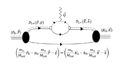
Figure 9: Diagrammatic representation of diagram (c).

For calculating the contribution of the form factor presented in Fig. 9, we start with the four-momentum integration as

$$\mathcal{F}^{(c)}(Q^{2})=(-ie\mathcal{Z})^{-1}\;\int_{k<\Lambda}\frac{d^{4}k}{(2\pi)^{4}}\;\int_{p<\Lambda}\frac{d^{4}p}{(2\pi)^{4}}\;(2\pi)^{4}$$

$$\times\delta(k_{0}-p_{0})\delta^{(3)}(\vec{k}-\vec{p}-\frac{m_{n}}{M_{tot}}\vec{Q})$$

$$\times(-ie\mathcal{Z})\;\Big{\{}i\;\mathcal{G}_{1}^{irr}(P_{0},\vec{P},p_{0},\vec{P})^{T}$$

$$\qquad\qquad\times\frac{i}{\frac{m_{n}}{M_{tot}}P_{0}-p_{0}-\frac{(\frac{m_{n}}{M_{tot}}\vec{P}-\vec{p})^{2}}{2m_{n}}+i\varepsilon}$$

$$\qquad\qquad\times\Big{[}-i\Sigma\Big{(}\frac{M_{1}}{M_{tot}}\bar{P}+\bar{p},\frac{M_{1}}{M_{tot}}\bar{K}+\bar{k}\Big{)}\Big{]}$$

$$\qquad\qquad\times iD_{1}\Big{(}\frac{M_{1}}{M_{tot}}K_{0}+k_{0},\frac{M_{1}}{M_{tot}}\vec{K}+\vec{k}\Big{)}$$

$$\qquad\qquad\times iD_{1}\Big{(}\frac{M_{1}}{M_{tot}}P_{0}+p_{0},\frac{M_{1}}{M_{tot}}\vec{P}+\vec{p}\Big{)}$$

$$\qquad\qquad\times i\;\mathcal{G}_{1}^{irr}(K_{0},\vec{K},k_{0},\vec{k})\Big{\}},$$ (B.7)

where $\Sigma\Big{(}\frac{M_{1}}{M_{tot}}\bar{P}+\bar{p},\frac{M_{1}}{M_{tot}}\bar{K}+\bar{k}\Big{)}$ is the $n\alpha$ bubble contribution in Fig. 9. One of the two four-momentum integrations in Eq. (B.7) is absorbed by a delta-function, so we obtain

$$\mathcal{F}^{(c)}(Q^{2}) = \int_{p<\Lambda}\frac{d^{4}p}{(2\pi)^{4}}\;\Big{\{}\mathcal{G}_{1}^{irr}(P_{0},\vec{P},p_{0},\vec{P})^{T}$$ (B.8)

$$\times \frac{i}{\frac{m_{n}}{M_{tot}}P_{0}-p_{0}-\frac{(\frac{m_{n}}{M_{tot}}\vec{P}-\vec{p})^{2}}{2m_{n}}+i\varepsilon}$$

$$\times \Big{[}-i\Sigma\Big{(}\frac{M_{1}}{M_{tot}}\bar{P}+\bar{p},\frac{M_{1}}{M_{tot}}\bar{K}+\bar{k}\Big{)}\Big{]}$$

$$\times D_{1}\Big{(}\frac{M_{1}}{M_{tot}}K_{0}+p_{0},\frac{M_{1}}{M_{tot}}\vec{K}+\vec{p}+\frac{m_{n}}{M_{tot}}\vec{Q}\Big{)}$$

$$\times D_{1}\Big{(}\frac{M_{1}}{M_{tot}}P_{0}+p_{0},\frac{M_{1}}{M_{tot}}\vec{P}+\vec{p}\Big{)}$$

$$\times \mathcal{G}_{1}^{irr}(K_{0},\vec{K},p_{0},\vec{p}+\frac{m_{n}}{M_{tot}}\vec{Q})\Big{\}}.$$

Using the rescaled four-momentum $\bar{s}=\frac{m_{n}}{2M_{tot}}\bar{Q}$ and the shifted loop momentum according to $\bar{p}\mapsto\bar{q}-\bar{s}$, we have

$$\mathcal{F}^{(c)}(Q^{2}) = \int_{q<\Lambda}\frac{d^{3}\vec{q}}{(2\pi)^{3}}\int_{-\infty}^{+\infty}\frac{dq_{0}}{2\pi}\;\Big{\{}\mathcal{G}_{1}^{irr}(P_{0},\vec{P},\bar{q}-\bar{s})^{T}$$ (B.9)

$$\times \frac{i}{\frac{m_{n}}{M_{tot}}P_{0}-q_{0}-\frac{(\frac{m_{n}}{M_{tot}}\vec{P}-\vec{q}+\vec{s})^{2}}{2m_{n}}+i\varepsilon}$$

$$\times \Big{[}-i\Sigma\Big{(}\frac{M_{1}}{M_{tot}}\bar{P}+\bar{q}-\bar{s},\frac{M_{1}}{M_{tot}}\bar{K}+\bar{q}+\bar{s}\Big{)}\Big{]}$$

$$\times D_{1}\Big{(}\frac{M_{1}}{M_{tot}}K_{0}+q_{0},\frac{M_{1}}{M_{tot}}\vec{K}+\vec{q}+\vec{s}\Big{)}$$

$$\times D_{1}\Big{(}\frac{M_{1}}{M_{tot}}P_{0}+q_{0},\frac{M_{1}}{M_{tot}}\vec{P}+\vec{q}-\vec{s}\Big{)}$$

$$\times \mathcal{G}_{1}^{irr}(K_{0},\vec{K},\bar{q}+\bar{s})\Big{\}}.$$

After performing the $q_{0}$ integration according to the pole $q_{0}=\frac{m_{n}}{M_{tot}}P_{0}-\frac{(\frac{m_{n}}{M_{tot}}\vec{P}-\vec{q}+\vec{s})^{2}}{2m_{n}}+i\varepsilon$, we obtain

$$\mathcal{F}^{(c)}(Q^{2}) = \int_{q<\Lambda}\frac{d^{3}\vec{q}}{(2\pi)^{3}}\;\Big{\{}\mathcal{G}_{1}^{irr}(P_{0},\vec{P},\bar{q}-\bar{s})^{T}\;$$ (B.10)

$$\times \Big{[}-i\Sigma\Big{(}\frac{M_{1}}{M_{tot}}\bar{P}+\bar{q}-\bar{s},\frac{M_{1}}{M_{tot}}\bar{K}+\bar{q}+\bar{s}\Big{)}\Big{]}$$

$$\times D_{1}\Big{(}\frac{M_{1}}{M_{tot}}K_{0}+q_{0},\frac{M_{1}}{M_{tot}}\vec{K}+\vec{q}+\vec{s}\Big{)}$$

$$\times D_{1}\Big{(}\frac{M_{1}}{M_{tot}}P_{0}+q_{0},\frac{M_{1}}{M_{tot}}\vec{P}+\vec{q}-\vec{s}\Big{)}$$

$$\times \mathcal{G}_{1}^{irr}(K_{0},\vec{K},\bar{q}+\bar{s})\Big{\}}.$$

Considering Eq. (LABEL:a1) and by substituting the pole $q_{0}$, we have

$$\mathcal{G}_{1}^{irr}(P_{0},\vec{P},\bar{q}-\bar{s})^{T} = \frac{1}{\sqrt{3}}\;\frac{m_{n}\;g_{1}^{2}}{\Lambda^{2}}\;\left|\beta\;H_{0}(\Lambda)\right|\;d(q,s,-x^{\prime})$$ (B.11)

$$- \sum_{i=0}^{1}\int_{0}^{\Lambda}dp\frac{p^{2}}{2\pi^{2}}\;\mathcal{G}_{i}^{irr}(E,p)\;\overline{D}_{i}(E,p)$$

$$\quad\times R_{i1}\Big{(}E,p,d(q,s,-x^{\prime})\Big{)},$$

$$\mathcal{G}_{1}^{irr}(K_{0},\vec{K},\bar{q}+\bar{s}) = \frac{1}{\sqrt{3}}\;\frac{m_{n}\;g_{1}^{2}}{\Lambda^{2}}\;\left|\beta\;H_{0}(\Lambda)\right|\;d(q,s,x^{\prime})$$ (B.12)

$$- \sum_{j=0}^{1}\int_{0}^{\Lambda}dk\frac{k^{2}}{2\pi^{2}}\;R_{1j}\Big{(}E,d(q,s,x^{\prime}),k\Big{)}$$

$$\quad\times\overline{D}_{j}(E,k)\;\mathcal{G}_{j}^{irr}(E,k),$$

with $d(q,s,\pm x^{\prime})=\sqrt{q^{2}+s^{2}\pm 2qsx^{\prime}}$ and the polar angle $x^{\prime}=\cos(\angle(\vec{Q},\vec{q}))$. Using Eq. (9), Eq. (21) and inserting the pole $q_{0}$, we can redefine the two propagators in Eq. (B.9) as

$$D_{1}\Big{(}\frac{M_{1}}{M_{tot}}K_{0}+q_{0},\frac{M_{1}}{M_{tot}}\vec{K}+\vec{q}+\vec{s}\Big{)}$$

$$\qquad\quad\qquad=\overline{D}_{1}\Big{(}E-\frac{m_{n}}{8M_{1}M_{tot}}Q^{2}-\frac{qQx^{\prime}}{2M_{1}},q\Big{)},$$

$$D_{1}\Big{(}\frac{M_{1}}{M_{tot}}P_{0}+q_{0},\frac{M_{1}}{M_{tot}}\vec{P}+\vec{q}-\vec{s}\Big{)}$$

$$\qquad\quad\qquad=\overline{D}_{1}\Big{(}E-\frac{m_{n}}{8M_{1}M_{tot}}Q^{2}+\frac{qQx^{\prime}}{2M_{1}},q\Big{)}.$$

B.3.1 Bubble diagram

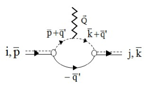
Figure 10: Diagrammatic representation of the bubble contribution $-i\Sigma(\bar{p},\bar{k})$.

We now calculate the term $-i\Sigma\Big{(}\frac{M_{1}}{M_{tot}}\bar{P}+\bar{q}-\bar{s},\frac{M_{1}}{M_{tot}}\bar{K}+\bar{q}+\bar{s}\Big{)}$ for the bubble diagram depicted in Fig. 10. For general incoming (outgoing) four-momenta $\bar{p}\;(\bar{k})$ and according to Eq. (4), we obtain

$$-i\Sigma(\bar{p},\bar{k}) = -\int\frac{d^{3}\vec{q^{\prime}}}{(2\pi)^{3}}\Big{(}i\frac{g_{1}}{2}\Big{)}^{2}$$

$$\times \Big{[}\frac{1}{\frac{q^{\prime 2}}{2m_{n}}+\frac{(\vec{k}+\vec{q^{\prime}})^{2}}{2m_{\alpha}}-k_{0}}\times\frac{1}{\frac{q^{\prime 2}}{2m_{n}}+\frac{(\vec{p}+\vec{q^{\prime}})^{2}}{2m_{\alpha}}-p_{0}}$$

$$\times (\vec{k}(1-r)+2\vec{q^{\prime}})_{j}(\vec{p}(1-r)+2\vec{q^{\prime}})_{i}\;\textrm{Tr}(S^{{\dagger}}_{j}S_{i})\Big{]}.$$

According to Eq. (6), we derive $\textrm{Tr}(S^{{\dagger}}_{j}S_{i})=\frac{4}{3}\delta_{ij}$. Furthermore, using the relation $\frac{1}{a_{1}a_{2}}=\int_{0}^{1}\frac{dx}{[a_{1}x+a_{2}(1-x)]^{2}}$ and defining the rescaled loop momentum $\vec{b}:=\frac{\vec{q^{\prime}}+\frac{\mu}{m_{\alpha}}[x\vec{p}+(1-x)\vec{k}]}{\frac{\mu}{m_{\alpha}}Q}$ and replacing our kinematics $\bar{p}\mapsto\frac{M_{1}}{M_{tot}}\bar{P}+\bar{q}-\bar{s}$ and $\bar{k}\mapsto\frac{M_{1}}{M_{tot}}\bar{K}+\bar{q}+\bar{s}$ in Eq. (LABEL:a11), we can obtain the following relation for the bubble contribution, $\Sigma$, as

$$- i\Sigma\Big{(}\frac{M_{1}}{M_{tot}}\bar{P}+\bar{q}-\bar{s},\frac{M_{1}}{M_{tot}}\bar{K}+\bar{q}+\bar{s}\Big{)}$$ (B.16)

$$=\frac{4}{3}\frac{\mu\;m_{\alpha}}{Q}g_{1}^{2}\int_{0}^{1}dx\int\frac{d^{3}\vec{b}}{(2\pi)^{3}}\Bigg{\{}\frac{1}{(b^{2}-A_{\left|\overline{q}-\overline{s}\right|,\left|\overline{q}+\overline{s}\right|}(x))^{2}}$$

$$\times\Bigg{[}\Big{(}\frac{M_{1}}{M_{tot}}\vec{K}+\vec{q}+\vec{s}\Big{)}(1-r)$$

$$\qquad+\frac{2\mu}{m_{\alpha}}\Big{(}Q\vec{b}-\Big{[}x\Big{(}\frac{M_{1}}{M_{tot}}\vec{P}+\vec{q}-\vec{s}\Big{)}$$

$$\qquad+(1-x)\Big{(}\frac{M_{1}}{M_{tot}}\vec{K}+\vec{q}+\vec{s}\Big{)}\Big{]}\Big{)}\Bigg{]}_{i}$$

$$\times\Bigg{[}\Big{(}\frac{M_{1}}{M_{tot}}\vec{P}+\vec{q}-\vec{s}\Big{)}(1-r)$$

$$\qquad+\frac{2\mu}{m_{\alpha}}\Big{(}Q\vec{b}-\Big{[}x\Big{(}\frac{M_{1}}{M_{tot}}\vec{P}+\vec{q}-\vec{s}\Big{)}$$

$$\qquad+(1-x)\Big{(}\frac{M_{1}}{M_{tot}}\vec{K}+\vec{q}+\vec{s}\Big{)}\Big{]}\Big{)}\Bigg{]}_{i}\Bigg{\}},$$

where

$$A_{\left|\overline{q}-\overline{s}\right|,\left|\overline{q}+\overline{s}\right|}(x)=x^{2}-x\Big{(}1+C_{\overline{P},\overline{q}-\overline{s}}-C_{\overline{K},\overline{q}+\overline{s}}\Big{)}-C_{\overline{K},\overline{q}+\overline{s}},$$

(B.17)

with

$$C_{\overline{P},\overline{q}-\overline{s}}=2\mu\Big{[}B_{2n}+\frac{(\vec{q}-\vec{s})^{2}}{2\tilde{\mu}}\Big{]}\Big{(}\frac{M_{1}}{2M_{tot}}\Big{)}^{2}\frac{1}{s^{2}},$$

$$C_{\overline{K},\overline{q}+\overline{s}}=2\mu\Big{[}B_{2n}+\frac{(\vec{q}+\vec{s})^{2}}{2\tilde{\mu}}\Big{]}\Big{(}\frac{M_{1}}{2M_{tot}}\Big{)}^{2}\frac{1}{s^{2}},$$ (B.18)

and $\tilde{\mu}=\frac{m_{n}M_{1}}{M_{tot}}$. Finally, after some derivations, the relation of the bubble contribution in Eq. (B.16) converts to

$$- i\Sigma\Big{(}\frac{M_{1}}{M_{tot}}\bar{P}+\bar{q}-\bar{s},\frac{M_{1}}{M_{tot}}\bar{K}+\bar{q}+\bar{s}\Big{)}$$ (B.19)

$$= \frac{4}{3}\frac{\mu m_{\alpha}}{Q}g_{1}^{2}\int_{0}^{1}dx\Bigg{\{}4\frac{\mu^{2}}{m_{\alpha}^{2}}Q^{2}\int\frac{d^{3}\vec{b}}{(2\pi)^{3}}\frac{b^{2}}{[b^{2}-A_{\left|\overline{q}-\overline{s}\right|,\left|\overline{q}+\overline{s}\right|}(x)]^{2}}$$

$$+16Qs\Big{(}\frac{\mu^{2}}{m_{\alpha}^{2}}\frac{M_{1}}{M_{tot}}\Big{)}\!(x^{2}\!-\!x)\!\int\!\frac{d^{3}\vec{b}}{(2\pi)^{3}}\frac{1}{[b^{2}-A_{\left|\overline{q}-\overline{s}\right|,\left|\overline{q}+\overline{s}\right|}(x)]^{2}}$$

$$+16\frac{\mu^{2}}{m_{\alpha}^{2}}s^{2}(\!x^{2}\!-x\!)\!\int\!\frac{d^{3}\vec{b}}{(2\pi)^{3}}\frac{1}{[b^{2}-A_{\left|\overline{q}-\overline{s}\right|,\left|\overline{q}+\overline{s}\right|}(x)]^{2}}$$

$$+4\Big{(}\frac{\mu^{2}}{m_{\alpha}^{2}}\frac{M_{1}^{2}}{M_{tot}^{2}}\Big{)}Q^{2}(\!x^{2}\!-\!x\!)\!\int\!\frac{d^{3}\vec{b}}{(2\pi)^{3}}\frac{1}{[b^{2}-A_{\left|\overline{q}-\overline{s}\right|,\left|\overline{q}+\overline{s}\right|}(x)]^{2}}\Bigg{\}}$$

$$= \frac{2i}{3\pi}\frac{\mu^{3}}{m_{\alpha}}g_{1}^{2}Q[-3I_{4}+I_{3}-I_{2}],$$

where the functions $I_{2}$, $I_{3}$ and $I_{4}$ in the last line are given using the relations

$$\int\frac{d^{3}\vec{b}}{(2\pi)^{3}}\frac{1}{[b^{2}-A_{\left|\overline{q}-\overline{s}\right|,\left|\overline{q}+\overline{s}\right|}(x)]^{2}}=\frac{i}{8\pi}\frac{1}{\sqrt{A_{\left|\overline{q}-\overline{s}\right|,\left|\overline{q}+\overline{s}\right|}(x)}},$$

(B.20)

and

$$\int\frac{d^{3}\vec{b}}{(2\pi)^{3}}\frac{b^{2}}{[b^{2}-A_{\left|\overline{q}-\overline{s}\right|,\left|\overline{q}+\overline{s}\right|}(x)]^{2}}=\frac{3i}{8\pi}\sqrt{A_{\left|\overline{q}-\overline{s}\right|,\left|\overline{q}+\overline{s}\right|}(x)},$$

(B.21)

as

$$I_{2} = \int_{0}^{1}dx\frac{x}{\sqrt{A_{\left|\overline{q}-\overline{s}\right|,\left|\overline{q}+\overline{s}\right|}(x)}}$$

$$= i\Big{(}\sqrt{C_{\overline{P},\overline{q}-\overline{s}}}-\sqrt{C_{\overline{K},\overline{q}+\overline{s}}}\Big{)}\!+\!\frac{(1+C_{\overline{P},\overline{q}-\overline{s}}-C_{\overline{K},\overline{q}+\overline{s}})}{2}I_{1},$$

$$I_{3} = \int_{0}^{1}dx\frac{x^{2}}{\sqrt{A_{\left|\overline{q}-\overline{s}\right|,\left|\overline{q}+\overline{s}\right|}(x)}}$$ (B.23)

$$= \frac{1}{4}\Big{[}(1+C_{\overline{K},\overline{q}+\overline{s}}-C_{\overline{P},\overline{q}-\overline{s}})i\sqrt{C_{\overline{P},\overline{q}-\overline{s}}}$$

$$+(1+C_{\overline{P},\overline{q}-\overline{s}}-C_{\overline{K},\overline{q}+\overline{s}})i\sqrt{C_{\overline{K},\overline{q}+\overline{s}}}\;\Big{]}$$

$$+\frac{1}{2}\Big{(}C_{\overline{K},\overline{q}+\overline{s}}+\frac{(1+C_{\overline{P},\overline{q}-\overline{s}}-C_{\overline{K},\overline{q}+\overline{s}})^{2}}{4}\Big{)}I_{1}$$

$$+(1+C_{\overline{P},\overline{q}-\overline{s}}-C_{\overline{K},\overline{q}+\overline{s}})i\Big{(}\sqrt{C_{\overline{P},\overline{q}-\overline{s}}}-\sqrt{C_{\overline{K},\overline{q}+\overline{s}}}\;\Big{)}$$

$$+\frac{(1+C_{\overline{P},\overline{q}-\overline{s}}-C_{\overline{K},\overline{q}+\overline{s}})^{2}}{4}I_{1},$$

$$I_{4} = \int_{0}^{1}dx\sqrt{A_{\left|\overline{q}-\overline{s}\right|,\left|\overline{q}+\overline{s}\right|}(x)}$$

$$= \frac{1}{4}\Big{[}(1+C_{\overline{K},\overline{q}+\overline{s}}-C_{\overline{P},\overline{q}-\overline{s}})i\sqrt{C_{\overline{P},\overline{q}-\overline{s}}}$$

$$+(1+C_{\overline{P},\overline{q}-\overline{s}}-C_{\overline{K},\overline{q}+\overline{s}})i\sqrt{C_{\overline{K},\overline{q}+\overline{s}}}\;\Big{]}$$

$$-\frac{1}{2}\Big{(}C_{\overline{K},\overline{q}+\overline{s}}+\frac{(1+C_{\overline{P},\overline{q}-\overline{s}}-C_{\overline{K},\overline{q}+\overline{s}})^{2}}{4}\Big{)}I_{1}.$$

The $I_{1}$ function in Eqs. (LABEL:a019)-(B.3.1) is defined by the expression

$$I_{1} = \int_{0}^{1}\frac{dx}{\sqrt{A_{\left|\overline{q}-\overline{s}\right|,\left|\overline{q}+\overline{s}\right|}(x)}}$$ (B.25)

$$= -i\Bigg{[}\arctan\Bigg{(}\frac{\frac{M_{tot}}{M_{1}}s+\frac{m_{\alpha}}{M_{1}}qx^{\prime}}{\sqrt{2\mu\Big{(}B_{2n}+\frac{(\vec{q}-\vec{s})^{2}}{2\tilde{\mu}}\Big{)}}}\Bigg{)}$$

$$\qquad+\arctan\Bigg{(}\frac{\frac{M_{tot}}{M_{1}}s-\frac{m_{\alpha}}{M_{1}}qx^{\prime}}{\sqrt{2\mu\Big{(}B_{2n}+\frac{(\vec{q}+\vec{s})^{2}}{2\tilde{\mu}}\Big{)}}}\Bigg{)}\Bigg{]}.$$

B.3.2 Final representation of ${F}^{(c)}(Q^{2})$

In the final step, by inserting Eqs. (B.11)-(B.3) into Eq. (B.10), we find

$$\mathcal{F}^{(c)}(Q^{2})=\;\int_{0}^{\Lambda}\Big{(}-\frac{p^{2}}{2\pi^{2}}\Big{)}\;dp\;\int_{0}^{\Lambda}\Big{(}-\frac{k^{2}}{2\pi^{2}}\Big{)}\;dk\;\vec{\mathcal{G}}^{irr}(p)^{T}$$

$$\times D(p)\;\Upsilon^{(c)}(Q,p,k)\;D(k)\;\vec{\mathcal{G}}^{irr}(k)$$

$$+2\int_{0}^{\Lambda}\Big{(}-\frac{p^{2}}{2\pi^{2}}\Big{)}dp\vec{\mathcal{G}}^{irr}(p)^{T}D(p)\vec{\Upsilon}^{(c)}(Q,p)+\Upsilon^{(c)}_{0}(Q),$$

(B.26)

where

$$\Upsilon^{(c)}_{ij}(Q,p,k) = \frac{1}{(2\pi)^{3}}\;\int_{0}^{\Lambda}q^{2}\;dq\;\int_{-1}^{1}dx^{\prime}\;\int_{0}^{2\pi}d\phi$$

$$\times\chi^{(c)}_{ij}(\frac{m_{n}}{2M_{tot}}Q,p,k,q,x^{\prime},\phi),$$

$$\Upsilon^{(c)}_{i}(Q,p) = \frac{1}{(2\pi)^{3}}\;\int_{0}^{\Lambda}q^{2}\;dq\;\int_{-1}^{1}dx^{\prime}\;\int_{0}^{2\pi}d\phi$$

$$\times\chi^{(c)}_{i}(\frac{m_{n}}{2M_{tot}}Q,p,q,x^{\prime},\phi),$$

$$\Upsilon^{(c)}_{0}(Q) = \frac{1}{(2\pi)^{3}}\int_{0}^{\Lambda}q^{2}dq\int_{-1}^{1}dx^{\prime}\int_{0}^{2\pi}d\phi$$ (B.27)

$$\times\chi^{(c)}_{0}(\frac{m_{n}}{2M_{tot}}Q,q,x^{\prime},\phi),$$

with the following relations

$$\chi^{(c)}_{ij}(\frac{m_{n}}{2M_{tot}}Q,q,x,p,k)=R_{i1}\Big{(}-B_{2n},p,d(q,s,-x^{\prime})\Big{)}$$

$$\qquad\times\overline{D}_{1}\Big{(}-B_{2n}\;-\;\frac{m_{n}}{8M_{1}M_{tot}}\;Q^{2}\;-\;\frac{qQx^{\prime}}{2M_{1}},q\Big{)}$$

$$\qquad\times\Big{[}-i\;\Sigma\Big{(}\frac{M_{1}}{M_{tot}}\bar{P}+\bar{q}-\bar{s},\frac{M_{1}}{M_{tot}}\bar{K}+\bar{q}+\bar{s}\Big{)}\Big{]}$$

$$\qquad\times\overline{D}_{1}\Big{(}-B_{2n}\;-\;\frac{m_{n}}{8M_{1}M_{tot}}\;Q^{2}\;+\;\frac{qQx^{\prime}}{2M_{1}},q\Big{)}$$

$$\qquad\times R_{1j}\Big{(}-B_{2n},d(q,s,x^{\prime}),k\Big{)},$$ (B.28)

$$\chi^{(c)}_{i}(\frac{m_{n}}{2M_{tot}}Q,p,q,x^{\prime},\phi)=\frac{1}{\sqrt{3}}\;\frac{m_{n}\;g_{1}^{2}}{\Lambda^{2}}\left|\beta H_{0}(\Lambda)\right|d(q,s,x^{\prime})$$

$$\qquad\times R_{i1}\Big{(}-B_{2n},p,d(q,s,-x^{\prime})\Big{)}$$

$$\qquad\times\overline{D}_{1}\Big{(}-B_{2n}\;-\;\frac{m_{n}}{8M_{1}M_{tot}}\;Q^{2}\;-\;\frac{qQx^{\prime}}{2M_{1}},q\Big{)}$$

$$\qquad\times\Big{[}-i\;\Sigma\Big{(}\frac{M_{1}}{M_{tot}}\bar{P}+\bar{q}-\bar{s},\frac{M_{1}}{M_{tot}}\bar{K}+\bar{q}+\bar{s}\Big{)}\Big{]}$$

$$\qquad\times\overline{D}_{1}\Big{(}-B_{2n}\;-\;\frac{m_{n}}{8M_{1}M_{tot}}\;Q^{2}\;+\;\frac{qQx^{\prime}}{2M_{1}},q\Big{)},$$ (B.29)

$$\chi^{(c)}_{0}(\frac{m_{n}}{2M_{tot}}Q,q,x^{\prime},\phi)=\frac{1}{\sqrt{3}}\frac{m_{n}g_{1}^{2}}{\Lambda^{2}}\left|\beta H_{0}(\Lambda)\right|d(q,s,-x^{\prime})$$

$$\qquad\times\overline{D}_{1}\Big{(}-B_{2n}\;-\;\frac{m_{n}}{8M_{1}M_{tot}}\;Q^{2}\;-\;\frac{qQx^{\prime}}{2M_{1}},q\Big{)}$$

$$\qquad\times\Big{[}-i\;\Sigma\Big{(}\frac{M_{1}}{M_{tot}}\bar{P}+\bar{q}-\bar{s},\frac{M_{1}}{M_{tot}}\bar{K}+\bar{q}+\bar{s}\Big{)}\Big{]}$$

$$\qquad\times\overline{D}_{1}\Big{(}-B_{2n}\;-\;\frac{m_{n}}{8M_{1}M_{tot}}\;Q^{2}\;+\;\frac{qQx^{\prime}}{2M_{1}},q\Big{)}$$

$$\qquad\times\frac{1}{\sqrt{3}}\;\frac{m_{n}\;g_{1}^{2}}{\Lambda^{2}}\;\left|\beta\;H_{0}(\Lambda)\right|\;d(q,s,x^{\prime}).$$ (B.30)

As it mentioned all calculations have been performed in Breit frame, so we have substituted $E=-B_{2n}$ in Eqs. (B.28)-(B.30) and drop this energy variable in $\vec{\mathcal{G}}^{irr}$ and matrix $D$ in Eq. (B.26).

B.4 Contribution $\mathcal{F}_{E}^{(d)}$

Diagram (d) in Fig. 5 is the same as diagram (c) by converting the $n\alpha$ bubble to the vertex of photon-$d_{1}$ coupling, therefore the contribution of the diagram (d) is given by

$$\mathcal{F}^{(d)}(Q^{2}) = \;\int_{0}^{\Lambda}\Big{(}-\frac{p^{2}}{2\pi^{2}}\Big{)}\;dp\;\int_{0}^{\Lambda}\Big{(}-\frac{k^{2}}{2\pi^{2}}\Big{)}\;dk$$ (B.31)

$$\quad\times\vec{\mathcal{G}}^{irr}(p)^{T}\;D(p)\;\Upsilon^{(d)}(Q,p,k)\;D(k)\;\vec{\mathcal{G}}^{irr}(k)$$

$$+2\int_{0}^{\Lambda}\Big{(}-\frac{p^{2}}{2\pi^{2}}\Big{)}\;dp\;\vec{\mathcal{G}}^{irr}(p)^{T}\;D(p)\;\vec{\Upsilon}^{(d)}(Q,p)$$

$$+\Upsilon^{(d)}_{0}(Q),$$

where

$$\Upsilon^{(d)}_{ij}(Q,p,k) = \frac{1}{(2\pi)^{3}}\;\int_{0}^{\Lambda}q^{2}\;dq\;\int_{-1}^{1}dx^{\prime}\;\int_{0}^{2\pi}d\phi$$

$$\quad\times\chi^{(d)}_{ij}(\frac{m_{n}}{2M_{tot}}Q,p,k,q,x^{\prime},\phi),$$

$$\vec{\Upsilon}^{(d)}_{i}(Q,p) = \frac{1}{(2\pi)^{3}}\;\int_{0}^{\Lambda}q^{2}\;dq\;\int_{-1}^{1}dx^{\prime}\;\int_{0}^{2\pi}d\phi$$

$$\quad\times\chi^{(d)}_{i}(\frac{m_{n}}{2M_{tot}}Q,p,q,x^{\prime},\phi),$$

$$\Upsilon^{(d)}_{0}(Q) = \frac{1}{(2\pi)^{3}}\;\int_{0}^{\Lambda}q^{2}\;dq\;\int_{-1}^{1}dx^{\prime}\;\int_{0}^{2\pi}d\phi$$ (B.32)

$$\quad\times\chi^{(d)}_{0}(\frac{m_{n}}{2M_{tot}}Q,q,x^{\prime},\phi),$$

with the following relations

$$\chi^{(d)}_{ij}(\frac{m_{n}}{2M_{tot}}Q,q,x^{\prime},p,k)=R_{i1}\Big{(}-B_{2n},p,d(q,s,-x^{\prime})\Big{)}$$

$$\qquad\times\overline{D}_{1}\Big{(}-B_{2n}\;-\;\frac{m_{n}}{8M_{1}M_{tot}}\;Q^{2}\;-\;\frac{qQx^{\prime}}{2M_{1}},q\Big{)}$$

$$\qquad\times\overline{D}_{1}\Big{(}-B_{2n}\;-\;\frac{m_{n}}{8M_{1}M_{tot}}\;Q^{2}\;+\;\frac{qQx^{\prime}}{2M_{1}},q\Big{)}$$

$$\qquad\times R_{1j}\Big{(}-B_{2n},d(q,s,x^{\prime}),k\Big{)},$$

$$\chi^{(d)}_{i}(\frac{m_{n}}{2M_{tot}}Q,p,q,x^{\prime},\phi)=\frac{1}{\sqrt{3}}\;\frac{m_{n}\;g_{1}^{2}}{\Lambda^{2}}\;\left|\beta\;H_{0}(\Lambda)\right|$$

$$\qquad\times d(q,s,x^{\prime})\;R_{i1}\Big{(}-B_{2n},p,d(q,s,-x^{\prime})\Big{)}$$

$$\qquad\times\overline{D}_{1}\Big{(}-B_{2n}\;-\;\frac{m_{n}}{8M_{1}M_{tot}}\;Q^{2}\;-\;\frac{qQx^{\prime}}{2M_{1}},q\Big{)}$$

$$\qquad\times\overline{D}_{1}\Big{(}-B_{2n}\;-\;\frac{m_{n}}{8M_{1}M_{tot}}\;Q^{2}\;+\;\frac{qQx^{\prime}}{2M_{1}},q\Big{)},$$

$$\chi^{(d)}_{0}(\frac{m_{n}}{2M_{tot}}Q,q,x^{\prime},\phi)=\frac{1}{\sqrt{3}}\;\frac{m_{n}\;g_{1}^{2}}{\Lambda^{2}}\;\left|\beta\;H_{0}(\Lambda)\right|$$

$$\qquad\times d(q,s,-x^{\prime})$$

$$\qquad\times\overline{D}_{1}\Big{(}-B_{2n}\;-\;\frac{m_{n}}{8M_{1}M_{tot}}\;Q^{2}\;-\;\frac{qQx^{\prime}}{2M_{1}},q\Big{)}$$

$$\qquad\times\overline{D}_{1}\Big{(}-B_{2n}\;-\;\frac{m_{n}}{8M_{1}M_{tot}}\;Q^{2}\;+\;\frac{qQx^{\prime}}{2M_{1}},q\Big{)}$$

$$\qquad\times\frac{1}{\sqrt{3}}\;\frac{m_{n}\;g_{1}^{2}}{\Lambda^{2}}\;\left|\beta\;H_{0}(\Lambda)\right|\;d(q,s,x^{\prime}).$$ (B.33)

References

- (1) S. Weinberg, Phys. Lett. B 251, 288 (1990); Nucl. Phys. B 363, 3 (1991).
- (2) M. Rho, Phys. Rev. Lett 66, 1275 (1991).
- (3) C. Ordóñez, and U. van Kolck, Phys. Lett. B 291, 459 (1992).
- (4) P. F. Bedaque, and U. van Kolck, Ann. Rev. Nucl. Part. Sci 52, 339 (2002).
- (5) S. R. Beane, P. F. Bedaque, W. C. Haxton, D. R. Phillips, and M. J. Savage, at the frontier of particle physics, 133-269 (World Scientific, Singapore,2001).
- (6) Nuclear Physics with Effective Field Theory II, ed. P. F. Bedaque, M.J. Savage, R. Seki, and U. van Kolck (World Scientific, Singapore, 1999);Nuclear Physics with Effective Field Theory, ed. R. Seki, U. van Kolck, and M. J. Savage (World Scientific, Singapore, 1998).
- (7) D. B. Kaplan, M. J. Savage, and M. B. Wise, Nucl. Phys. B 534, 329 (1998).
- (8) U. van Kolck, Nucl. Phys. A 645, 273 (1999).
- (9) J. W. Chen, G. Rupak, and M. J. Savage, Nucl. Phys. A 653, 386 (1999).
- (10) K. Riisager, Rev. Mod. Phys. 66, 1105 (1994).
- (11) M. V. Zhukov, B. V. Danilin, D. V. Fedorov, J. M. Bang, I. J. Thompson, and J. S. Vaagen, Phys. Rep. 231, 151 (1993).
- (12) P. G. Hansen, A. S. Jensen, and B. Jonson, Ann. Rev. Nucl. Part. Sci 45, 591 (1995).
- (13) A. S. Jensen, K. Riisager, D. V. Fedorov, and E. Garrido, Rev. Mod. Phys. 76, 215 (2004).
- (14) D. L. Canham, and H. -W. Hammer, Eur. Phys. J. A 37, 367 (2008).
- (15) D. L. Canham, and H. -W. Hammer, Nucl. Phys. A 836, 275 (2010).
- (16) G. Rupak, and R. Higa, Phys. Rev. Lett 106, 222501 (2011).
- (17) L. Fernando, R. Higa, and G. Rupak, Eur. Phys. J. A 48, 24 (2012).
- (18) X. Zhang, K. M. Nollett, and D. R. Phillips, Phys. Rev. C 89, 024613 (2014).
- (19) H. Hammer, and D. Phillips, Nucl. Phys. A 865, 17 (2011).
- (20) P. Hagen, H.-W. Hammer, and L. Platter, Eur. Phys. J. A 49, 118 (2013).
- (21) J. Vanasse, Phys. Rev. C 95, 024318 (2017).
- (22) H. -W. Hammer, C. Ji, and D. R. Phillips, J. Phys. G: Nucl. Part. Phys. 44, 103002 (2017).
- (23) C. Ji, C. Elster, and D. R. Phillips, Phys. Rev. C 90, 044004 (2014).
- (24) C. A. Bertulani, H. -W. Hammer, and U. van Kolck, Nucl. Phys. A 712, 37 (2002).
- (25) P. F. Bedaque, H. -W. Hammer, U. van Kolck, Phys. Lett. B 569, 159 (2003).
- (26) M. M. Arani, M. Radin, and S. Bayegan, Prog. Theor. Exp. Phys. 9, 093D07 (2017).
- (27) M. G¨obel, H. Hammer, C. Ji, and D. Phillips, Few-Body Syst. 60, 61 (2019).
- (28) J. Rotureau, and U. van Kolck, Few-Body Syst. 54, 725 (2013).
- (29) R. A. Arndt, D. D. Long, and L. D. Roper, Nucl. Phys. A 209, 429 (1973).
- (30) I. Tanihata, D. Hirata, T. Kobayashi, S. Shimoura, K.Sugimoto, and H. Toki, Phys. Lett. B 289, 261 (1992).
- (31) J. Vanasse, Phys. Rev. C 95, 024002 (2017).
- (32) D. B. Kaplan, M. J. Savage, and M. B. Wise, Phys. Rev. C 59, 617 (1999).
- (33) J. Vanasse, Phys. Rev. C 98, 034003 (2018).
- (34) S. Kopecky, J. A. Harvey, N. W. Hill, M. Krenn, M. Pernicka, P. Riehs, and S. Steiner, Phys. Rev. C 56, 2229 (1997).
- (35) E. Ryberg Ch. Forssn, and L. Platter, Few-Body Syst. 58, 143 (2017).
- (36) A. N. Antonov, D. N. Kadrev, M. K. Gaidarov, E. Moya de Guerra, P. Sarriguren, J. M. Udias, V. K. Lukyanov, E. V. Zemlyanaya, and G. Z. Krumova, Phys. Rev. C 72, 044307 (2005).
- (37) I. Sick, Phys. Rev. C 77, 041302(R) (2008).
- (38) L.-B. Wang, P. Mueller, K. Bailey, G. W. F. Drake, J. P. Greene, D. Henderson, R. J. Holt, R. V. F. Janssens, C. L. Jiang, Z.-T. Lu, T. P. O’Connor, R. C. Pardo, K. E. Rehm, J. P. Schiffer, and X. D. Tang, Phys. Rev. Lett. 93, 142501 (2004).
- (39) I. Sick, J. Phys. Chem. Ref. Data 44, 031213 (2015).
- (40) M. Brodeur, T. Brunner, C. Champagne, S. Ettenauer, M. J. Smith, A. Lapierre, R. Ringle, V. L. Ryjkov, S. Bacca, P. Delheij, G.W. F. Drake, D. Lunney, A. Schwenk, and J. Dilling, Phys. Rev. Lett 108, 052504 (2012).
- (41) S. Karataglidis, P. J. Dortmans, K. Amos, and C. Bennhold, Phys. Rev. C 61, 024319 (2000).
- (42) S. C. Pieper, and R. B. Wiringa, Annu. Rev. Nucl. Part. Sci. 51, 53 (2001).
- (43) S. König, H. W. Grießhammer, and H.-W. Hammer, J. Phys. G: Nucl. Part. Phys. 42(4), 045101 (2015).