Spatio-temporal correlations in 3D homogeneous isotropic turbulence

Abstract

We use Direct Numerical Simulations (DNS) of the forced Navier-Stokes equation for a 3-dimensional incompressible fluid in order to test recent theoretical predictions. We study the two- and three-point spatio-temporal correlation functions of the velocity field in stationary, isotropic and homogeneous turbulence. We compare our numerical results to the predictions from the Functional Renormalization Group (FRG) which were obtained in the large wavenumber limit. DNS are performed at various Reynolds numbers and the correlations are analyzed in different time regimes focusing on the large wavenumbers. At small time delays, we find that the two-point correlation function decays as a Gaussian in the variable $kt$ where $k$ is the wavenumber and $t$ the time delay. The three-point correlation function, determined from the time-dependent advection-velocity correlations, also follows a Gaussian decay at small $t$ with the same prefactor as the one of the two-point function. These behaviors are in precise agreement with the FRG results, and can be simply understood as a consequence of sweeping. At large time delays, the FRG predicts a crossover to an exponential in $k^{2}t$, which we were not able to resolve in our simulations. However, we analyze the two-point spatio-temporal correlations of the modulus of the velocity, and show that they exhibit this crossover from a Gaussian to an exponential decay, although we lack of a theoretical understanding in this case. This intriguing phenomenon calls for further theoretical investigation.

I Introduction

Characterizing the statistical properties of a turbulent flow is one of the main challenges to achieve a complete theoretical understanding of turbulence. Space-time correlations are at the heart of statistical theories of turbulence, and have been studied and modeled for many decades, both in the Eulerian and Lagrangian frameworks Wallace (2014); He, Jin, and Yang (2017). One of the earliest insights was provided by Taylor’s celebrated analysis of single particle dispersion by an isotropic turbulent flow Taylor (1922). The understanding of the behavior of turbulent fluctuations both in space and time is essential for many problems in fluid mechanics where the multiscale temporal dynamics plays a key role, such as particle-laden turbulence, propagation of waves in a turbulent medium or turbulence-generated noise in compressible flows He, Jin, and Yang (2017). Space-time correlations are also central for many closure schemes, such as the direct-interaction Approximation (DIA) elaborated by Kraichnan Kraichnan (1964), or the eddy damped quasi-normal Markovian (EDQNM) approximation les (2008). The accurate description of the spatio-temporal correlations is crucial for developing time-accurate large-eddy simulation (LES) turbulence models, as well as for the analysis of experimental data, for example, to assess the validity and corrections to the Taylor’s frozen flow model used for time-to-space conversion of measurements.

A fundamental ingredient to understand the temporal behavior of turbulent flows in the Eulerian frame is the sweeping effect, which was early identified in References Heisenberg, 1948; Kraichnan, 1959, 1964; Tennekes, 1975. The random sweeping effect results from the random advection of small-scale velocities by the large-scale energy-containing eddies, even in the absence of mean flow. This random sweeping was anticipated to induce a Gaussian decay in the variable $tk$, where $k$ is the wavenumber and $t$ the time delay, of the two-point correlations of the Eulerian velocity field, based on simplified models of advection Kraichnan (1964). However, at the theoretical level, the effect of sweeping also induces, in the original formulation of DIA, a $k^{-3/2}$ decay of the energy spectrum in the inertial range instead of the Kolmogorov $k^{-5/3}$ scaling. This led Kraichnan to a complete reformulation of his theory using Lagrangian space-time correlations instead of Eulerian ones. The dependence of the two-point correlation function in $k^{2}t^{2}$ predicted from sweeping has been observed and confirmed in numerous numerical simulations (Orszag and Patterson, 1972; Sanada and Shanmugasundaram, 1992; Chen and Kraichnan, 1989; He, Wang, and Lele, 2004; Favier, Godeferd, and Cambon, 2010; Canet et al., 2017) and also in experiments (Poulain et al., 2006). A notable consequence of this dependence in the product $kt$ is that the frequency energy spectrum of Eulerian velocities exhibits a $\omega^{-5/3}$ decay, instead of the $\omega^{-2}$ expected from K41 scaling Chevillard et al. (2005).

The random sweeping hypothesis is also a part of the elliptic approximation that provides a model for spatio-temporal correlation in turbulent shear flows He and Zhang (2006) combining the decorrelation effect of the sweeping by large scales and the convection by the mean flow, and provides a correction to Taylor frozen-flow model. The elliptic approximation model has been tested in numerical simulations and experimental measurements in Rayleigh-Bénard convection flows He, Jin, and Yang (2017). In Ref. Wilczek and Narita, 2012 a model of spatio-temporal spectrum of turbulence is proposed in the presence of a mean flow Kraichnan (1964) departing from the Kraichnan’s advection problem, which is consistent with the elliptical model. Fewer studies address multi-point correlations, although they are used as part of closure models Monin and Yaglom (2013). An expression for the three-point correlation function in a specific wave-vector and time configuration was obtained within the DIA Kraichnan (1959, 1964), and multi-point correlation functions were studied numerically in Ref. Biferale, Calzavarini, and Toschi, 2011.

Although the random sweeping effect is phenomenologically known for a long time, and the models based on it provide satisfactory descriptions, the theoretical justification of the hypothesis of random sweeping directly from the Navier-Stokes equation has remained a challenging task. The application of the renormalization group approach to turbulence developed by Yakhot et al. led to the conclusion that the sweeping effect on space-time correlations must be smallYakhot, Orszag, and She (1989), which is not in agreement with the $\omega^{-5/3}$ Eulerian spectrum. This result and its validity are discussed in the Ref. Chen and Kraichnan, 1989. In another work Drivas et al. (2017) the effect of the random sweeping was estimated with the use of equations of band-passed velocity advected by a large scale velocity. This work demonstrated that the random sweeping plays a dominant role in the Navier-Stokes dynamics at small scales.

Recently, a theoretical progress has been achieved using Functional Renormalization Group (FRG), which has yielded the general form of any multi-point correlation (and response) function in the limit of large wave-numbers. These expressions are established in the Eulerian frame, in a rigorous and systematic way. For the two-point space-time correlations, the Gaussian decay in $tk$ is recovered for small time delays $t$, while a crossover to a slower exponential decay in $t$ is predicted at large time delays. Similar results are obtained for any generic correlations involving an arbitrary number of space-time points. While the Gaussian regime is known to originate from sweeping, the exponential large-delay regime was not yet predicted. We show in this work that this behavior can also be derived from the original Taylor and Kraichnan’s arguments, which provide a clear physical interpretation of this result.

The aim of this work is to make precision tests of the FRG results using Direct Numerical Simulations (DNS) of the forced Navier-Stokes equation. We analyze the two-point and three-point correlations and accurately confirm the FRG prediction in the small-time regime. Even though the long-time regime remains elusive in the simulations data due to the weakness of the signal amplitude in this regime and the lack of statistics, we unveil a very similar crossover from a Gaussian to an exponential decay in the correlations of the modulus of the velocity field. However, this observation lacks a theoretical explanation so far.

The paper is organized as follows. In Sec. II, we briefly introduce the functional and nonperturbative renormalization group (FRG) framework and review the theoretical predictions stemming from it on the time dependence of multi-point correlation functions. We also provide a heuristic argument allowing one to grasp the physical content of these results. We present in Sec. III the results of our DNS analysis. We analyze the small delay regime of the two-point correlation functions in the Sec. III.1 and that of the three-point correlation function in the Sec. III.2. The temporal behavior of the two-point correlation of the modulus of the velocity is discussed in the Sec. III.3.

II Theoretical framework

II.1 Theoretical results from functional renormalization group

The FRG is a versatile method well-developed since the early 1990’s and used in a wide range of applications, both in high-energy physics (quantum gravity and QCD), condensed matter, quantum many-particle systems and statistical mechanics, including disordered and nonequilibrium problems (see References Berges, Tetradis, and Wetterich, 2002; Kopietz, Bartosch, and Schütz, 2010; Delamotte, 2012; Dupuis et al., 2020 for reviews). This method has been employed in particular to study the incompressible 3D Navier-Stokes equation in several works Tomassini (1997); Mejía-Monasterio and Muratore-Ginanneschi (2012); Canet, Delamotte, and Wschebor (2016); Canet et al. (2017); Tarpin, Canet, and Wschebor (2018); Tarpin et al. (2019). We here focus on a recent result concerning the spatio-temporal dependence of multi-point correlation functions of the turbulent velocity field in homogeneous, isotropic and stationary conditions. The detailed derivation of the theoretical results can be found in Ref. Tarpin, Canet, and Wschebor, 2018; it relies on an expansion at large wavenumbers of the exact FRG flow equations. The field theory arising from the stochastically forced Navier-Stokes equation possesses extended symmetries (in particular the time-dependent Galilean symmetry) which allow one to obtain the exact leading term of this expansion. We give below the ensuing expressions, before providing their intuitive physical interpretation in the Sec. II.2.

We are first interested in the two-point correlation function of the velocity expressed in the time-delay$-$wavevector mixed coordinates $(t,\vec{k})$, defined as

$$C^{(2)}(t,\vec{k}) \equiv\text{FT}\left[\left<u_{i}(t_{0},\vec{r}_{0})u_{i}(t_{0}+t,\vec{r}_{0}+\vec{r})\right>\right]$$ (1)

$$=\left<\hat{u}_{i}(t_{0},\vec{k})\hat{u}^{*}_{i}(t_{0}+t,\vec{k})\right>$$

where FT denotes the spatial Fourier transform. According to the FRG result, this function takes the following form for large wavenumbers $k=|\vec{k}|$ and small time delays:

$$C^{(2)}_{S}(t,\vec{k}) =C_{S}\epsilon^{2/3}k^{-11/3}\exp\Big{\{}-\alpha_{S}(L/\tau_{0})^{2}t^{2}k^{2}\Big{\}}\quad$$ (2)

and in the regime of large time delays:

$$C^{(2)}_{L}(t,\vec{k})=C_{L}\epsilon^{2/3}k^{-11/3}\exp\left\{-\alpha_{L}(L^{2}/\tau_{0})|t|k^{2}\right\}$$ (3)

with $\epsilon$ the energy dissipation rate, $L$ the integral length scale, $\tau_{0}=(L^{2}/\epsilon)^{1/3}$ the eddy-turnover time at the integral scale, and $\alpha_{S,L}$ and $C_{S,L}$ nonuniversal constants – the subscript $S$ and $L$ standing for ‘short time’ and ‘long time’ respectively. This expression conveys that the velocity field decorrelates at small time delays as a Gaussian of the variable $tk$, whereas at large time delays, the decay of the correlation function crosses over to an exponential in $t$. As mentioned in the introduction, the Gaussian behavior at small $t$ is well-known from experimental data and numerical simulations and interpreted as a consequence of the random sweeping effect. It turns out that the exponential decay at large $t$ can also be simply understood in a similar framework, as discussed in the Sec. II.2.

Let us comment on the domain of validity of these results. The factors in curly brackets in Eqs. (2) and (3) are exact in the limit of large wavenumber $k\gg L^{-1}$, which means that the corrections to these terms are at most of order ${\cal O}(k)$. We can quantify more precisely where this limit is reached using our DNS data. In contrast, the terms in front of the exponential in Eqs. (2) and (3) are not exact in these expressions, as they can be corrected by higher-order contributions neglected in the large wavenumber expansion. Otherwise stated, these expressions do not account for intermittency corrections on the exponent 11/3, which merely corresponds to K41 scaling.

The FRG theory yields a more general result: the spatio-temporal dependence of any multi-point correlation functions of the turbulent velocity field in the limit of large wavenumbers Tarpin, Canet, and Wschebor (2018). We concentrate in this work on the three-point correlation function, defined as

$$C^{(3)}_{\alpha\beta\gamma}(t_{1},\vec{k}_{1},t_{2},\vec{k}_{2})\equiv$$

$$\text{FT}\left[\left<u_{\alpha}(t_{0}+t_{1},\vec{r}_{0}+\vec{r}_{1})u_{\beta}(t_{0}+t_{2},\vec{r}_{0}+\vec{r}_{2})u_{\gamma}(t_{0},\vec{r}_{0})\right>\right]$$

$$=\left<\hat{u}_{\alpha}(t_{0}+t_{1},\vec{k}_{1})\hat{u}_{\beta}(t_{0}+t_{2},\vec{k}_{2})\hat{u}^{*}_{\gamma}(t_{0},\vec{k}_{1}+\vec{k}_{2})\right>$$ (4)

where translational invariances in space and time follow from the assumptions of homogeneity and stationarity. In the limit where all the wavenumbers $k_{1}$, $k_{2}$, $|\vec{k}_{1}+\vec{k}_{2}|$ are large, the FRG calculation leads to the following form at small time delays $t_{1}$ and $t_{2}$

$$C^{(3)}_{\alpha\beta\gamma}(t_{1},\vec{k}_{1},t_{2},\vec{k}_{2})=$$

$$C^{(3)}_{\alpha\beta\gamma}(0,\vec{k}_{1},0,\vec{k}_{2})\exp\left\{-\alpha_{S}(L/\tau_{0})^{2}\left|\vec{k}_{1}t_{1}+\vec{k}_{2}t_{2}\right|^{2}\right\}$$ (5)

with $\alpha_{S}$ the same constant as in Eq. (2). Note that a similar expression as Eq. (3) is also available for large time delays, but it is not considered here since it is out of reach of our simulations. In this work, we consider the simplified case $t=t_{1}=t_{2}$, thus aiming at testing the theoretical form

$$C^{(3)}_{\alpha\beta\gamma}(t,\vec{k}_{1},t,\vec{k}_{2})\sim\exp\left\{-\alpha_{S}(L/\tau_{0})^{2}\left|\vec{k}_{1}+\vec{k}_{2}\right|^{2}t^{2}\right\}.$$ (6)

One hence expects to observe that the three-point correlation functions at large wavenumbers are also Gaussian functions of a variable $|\vec{k}_{1}+\vec{k}_{2}|t$ for small time delays $t$, with the same prefactor $\alpha_{S}$ as in the two-point correlation functions.

Let us emphasize that similar results hold for any $n$-point correlation functions at large wavenumbers, and are valid for arbitrary time regimes, although for intermediate times the expressions take a more complicated integral form Tarpin, Canet, and Wschebor (2018). Their status is generically the same as discussed above for the two-point correlations: The leading terms in the exponentials are exact in the limit of large wavenumbers, whereas the prefactors of these exponentials are not. Let us now give a simple physical interpretation of these results.

II.2 Physical interpretation

The short-time predictions for time-dependence of two-point velocity correlations (2) and of three-point correlations (5) were both given in an early analysis of Eulerian sweeping effects by Kraichnan Kraichnan (1964). As we show now, the novel prediction of long-time exponential decay (3) and similar long-time decay of general multi-point correlations were implicit in that earlier analysis, but unrecognized at the time. Both short-time and long-time decay regimes can be obtained from the following Lagrangian expression for the Eulerian velocity field

$$u_{i}(t,\vec{r})=\exp_{\to}[-\vec{\xi}(t,\vec{r}|t_{0})\cdot\vec{\nabla}]u_{i}(t_{0},\vec{r})$$

$$+\int_{t_{0}}^{t}ds\ \exp_{\to}[-\vec{\xi}(t,\vec{r}|s)\cdot\vec{\nabla}]\left[\nu\nabla^{2}u_{i}(s,\vec{r})-\nabla_{i}p(s,\vec{r})\right].$$ (7)

This is equation (7.7) in the paper of Kraichnan Kraichnan (1964) when specialized to $s=t$ there (and with a minor typo corrected in the final term). Here $p(t,\vec{r})$ is the pressure, $\vec{\xi}(t,\vec{r}|s)=\vec{r}-\vec{X}(t,\vec{r}|s)$ is the Lagrangian displacement vector, where

$$\frac{d}{ds}\vec{X}(t,\vec{r}|s)=\vec{u}(s,\vec{X}(t,\vec{r}|s)),\quad\vec{X}(t,\vec{r}|t)=\vec{r}$$ (8)

defines the position $\vec{X}(t,\vec{r}|s)$ at time $s$ of the Lagrangian fluid particle located at position $\vec{r}$ at time $t.$ Finally $\exp_{\to}[-\vec{\xi}(t,\vec{r}|s)\cdot\vec{\nabla}]$ denotes an operator-ordered exponential with all gradients $\vec{\nabla}$ ordered to the right and thus not acting upon the $\vec{r}$-dependence in $\vec{\xi}(t,\vec{r}|s)$. The intuitive meaning of equation (7) is that it “states that the velocity field at later times is the result of self-convection of the initial velocity field, together with convection of all of the velocity increments induced at later times by viscous and pressure forces” Kraichnan (1964).

The formula (7) yields both of the FRG predictions (2) and (3) when some plausible statistical and dynamical assumptions are introduced. First, the displacement field $\vec{\xi}$ is expected to vary more slowly in space and time than the gradients of velocity $\vec{u}$ and of pressure $p$ that result from the action of the exponential operator. Slowness in time allows one to factor out the exponential as

$$u_{i}(t,\vec{r})=\exp_{\to}[-\vec{\xi}(t,\vec{r}|t_{0})\cdot\vec{\nabla}]\times$$

$$\Big{\{}u_{i}(t_{0},\vec{r})+\int_{t_{0}}^{t}ds\ \left[\nu\nabla^{2}u_{i}(s,\vec{r})-\nabla_{i}p(s,\vec{r})\right]\Big{\}}.$$ (9)

and slowness in space allows the Fourier transform to be evaluated as

$$\hat{u}_{i}(t,\vec{k})=\exp[-i\vec{\xi}(t,\vec{r}|t_{0})\cdot\vec{k}]\times$$

$$\Big{\{}\hat{u}_{i}(t_{0},\vec{k})-\int_{t_{0}}^{t}ds\ \left[\nu k^{2}\hat{u}_{i}(s,\vec{k})+k_{i}\hat{p}(s,\vec{k})\right]\Big{\}}.$$ (10)

The next assumption is that the displacement field $\vec{\xi}$ is almost statistically independent of the Fourier-transformed velocity fields at the initial time $t_{0}$, so that by the definition (1)

$$C^{(2)}(t,\vec{k})=\langle\exp[-i\vec{\xi}(t,\vec{r}|0)\cdot\vec{k}]\rangle\Big{\{}C^{(2)}(0,\vec{k})+{\cal O}(|t|)\Big{\}}.$$ (11)

Finally, since the Lagrangian displacement is dominated by the largest scales of the turbulent flow, which have nearly Gaussian statistics, it is plausible that $\vec{\xi}$ is also an approximately normal random field, so that

$$C^{(2)}(t,\vec{k})=\exp\left[-\frac{1}{2}\langle|\vec{\xi}(t,\vec{r}|0)|^{2}\rangle k^{2}\right]\Big{\{}C^{(2)}(0,\vec{k})+{\cal O}(|t|)\Big{\}}.$$ (12)

According to this argument, the 2-point velocity correlation undergoes a rapid decay in the time-difference $t$ which arises from an average over rapid oscillations in the phases of Fourier modes due to sweeping, or “convective dephasing”Kraichnan (1964).

The variance of the Lagrangian displacement in the exponent of (12) was the subject of a classical study by Taylor Taylor (1922) on 1-particle turbulent dispersion. Exploiting the expression

$$\vec{\xi}(t,\vec{r}|0)=\int_{0}^{t}\vec{u}(t,\vec{r}|s)\ ds,$$ (13)

two regimes were found:

$$\langle|\vec{\xi}(t,\vec{r}|0)|^{2}\rangle\sim\left\{\begin{array}[]{ll}u_{RMS}^{2}t^{2}&|t|\ll\tau_{0}\cr 2D|t|&|t|\gg\tau_{0}\end{array}\right.$$ (14)

where the early-time regime corresponds to ballistic motion with the rms velocity $u_{RMS}$ and the long-time regime corresponds to diffusion with a turbulent diffusivity $D\propto u_{RMS}^{2}\tau_{0}.$ Using the relation $u_{RMS}\propto L/\tau_{0}$ and the result (12) for the 2-point velocity correlation, these two regimes of 1-particle turbulent dispersion correspond exactly to the short-time scaling (2) and the long-time scaling (3) predicted by FRG, with $\frac{1}{2}u_{RMS}^{2}=\alpha_{S}(L/\tau_{0})^{2}$ and $D=\alpha_{L}L^{2}/\tau_{0}.$ To make more precise contact with the FRG analysis, one can introduce the temporal Fourier transform

$$\vec{v}(t,\vec{r};\omega)=\int ds\ e^{i\omega s}\vec{u}(t,\vec{r}|s)$$ (15)

and the corresponding (Lagrangian) frequency spectrum $\langle\vec{v}(\omega)\cdot\vec{v}(\omega^{\prime})\rangle=E(\omega)\delta(\omega+\omega^{\prime}).$ It is then easy to see that the displacement variance in (14) can be written as

$$\langle|\vec{\xi}(t,\vec{r}|0)|^{2}\rangle=\frac{1}{\pi}\int d\omega\ \frac{1-\cos(\omega t)}{\omega^{2}}E(\omega)$$ (16)

in terms of the velocity spectrum. This formula should be compared with the leading-order FRG flow equation (30) of Tarpin et al. Tarpin, Canet, and Wschebor (2018) obtained in the limit of large wavenumber $|\vec{k}|$

$$\kappa\partial_{\kappa}\ln C_{\kappa}^{(2)}(t,\vec{k})=\frac{2}{3}|\vec{k}|^{2}\int d\omega\ \frac{1-\cos(\omega t)}{\omega^{2}}J_{\kappa}(\omega)$$ (17)

where the common factor inside the two frequency integrals yields identical short-time and long-time power-law asymptotics ($\propto t^{2}$ and $\propto t$, resp.) in both expressions (16) and (17).

The above arguments can obviously be applied to general multi-point velocity correlations, yielding similar results. They provide an intuitive physical interpretation of the two scaling regimes of the FRG results Tarpin, Canet, and Wschebor (2018), with time-decay corresponding to a convective dephasing mechanism. In particular, the long-time exponential decay is suggested to arise from the diffusive linear growth in the position variance of a Lagrangian particle advected by homogeneous turbulence. This long-time exponential decay regime appears to be a novel prediction of the FRG approach. For example, it is quite distinct from the instantaneous exponential decay of the 2-point velocity correlator predicted by Rayleigh-Ritz analysis with a $K$-$\epsilon$ closure Eyink and Wray (1998), which occurs on very short time-scale before convective dephasing can act and which is interpreted as an eddy-viscosity effect. Needless to say, the FRG derivation of (2) and (3) is considerably more systematic and controlled than the heuristic argument presented in this section.

III Results of direct numerical simulations

We perform direct numerical simulations (DNS) of a stationary 3D incompressible homogeneous and isotropic turbulent flow. The computation domain represents a cube of size $2\pi$ with periodic boundary conditions. We use five values of the Taylor-scale Reynolds number: $R_{\lambda}=40,60,90,160,250$ with corresponding spatial grid size $N^{3}=64^{3},128^{3},256^{3},512^{3},1024^{3}$ (see Table 1). The spatial resolution of all simulations fulfills the condition $k_{max}\eta\simeq 1.5$, where $k_{max}=N/2$ is the maximal wavenumber in the simulation and $\eta$ is the Kolmogorov length scale. The incompressible Navier-Stokes equation is solved numerically with the use of a pseudospectral method in space Canuto (2007) and a second order Runge-Kutta scheme of time advancement. To achieve a statistically stationary state, the velocity field is randomly forced at large scales Alvelius (1999). We perform a de-aliasing with the use of the polyhedral truncation method Canuto (2007).

$R_{\lambda}$	N	$\nu$	$u_{RMS}$	$\tau_{0}$	$\Delta t$	$\Delta T_{w}$	$N_{t}$	$K_{c}L$
40	64	$10^{-4}$	0.0059	245	0.9	400	1008	14.6
60	128	$10^{-4}$	0.0147	134	0.1	75	665	23.7
90	256	$10^{-4}$	0.0375	45.3	0.03	10.0	624	42.5
160	512	$10^{-4}$	0.0974	19.0	0.005	1.0	322	74.4
250	1024	$10^{-4}$	0.2482	7.24	0.001	0.2	33	144

Table 1: Parameters of simulations for the analysis of two-point and three-point correlations at small time delays. $R_{\lambda}$ - Taylor-scale Reynolds number, $N$ - spatial grid resolution, $\nu$ - kinematic viscosity, $u_{RMS}$ - root mean square velocity, $\tau_{0}$ - eddy turnover time at the integral scale, $\Delta t$ - simulation time step, $\Delta T_{w}$ - width of a time window of correlation observation, $N_{t}$ - number of recorded time windows, $K_{c}L$- nondimensional cut-off wavenumber of the scale decomposition.

III.1 Two-point spatio-temporal correlations at small time delays

Once the simulations reach a statistically steady state, we compute the velocity correlation functions with the following method: At a chosen time $t_{0}$ we store the spectral 3D vector velocity field in the memory. At the next iterations the updated velocity field at time $t_{0}+i\Delta t$ is multiplied point-wise by the velocity field at time $t_{0}$. Since the velocity field is statistically isotropic, the two-point velocity correlation function is computed by averaging over spherical spectral shells $S_{n}$ of thickness $\Delta k=1$ so that $\vec{k}\in S_{n}\ \text{if}\ n-1<\big{|}\vec{k}\big{|}<n,n=1,..,N/2$. After a certain number of time iterations, when the magnitude of the correlations at all scales of interest is close to zero, the reference time $t_{0}$ is redefined as the current time, and the reference velocity field in the memory is updated. The resulting correlation function is averaged over time windows with different reference times $t_{0}$, and the real part is taken:

$$\bar{C}^{(2)}(t,k)=\frac{1}{N_{t}}\sum_{j=1}^{N_{t}}\frac{1}{M_{n}}\sum_{\vec{k}\in S_{n}}{\mathrm{Re}}\left[\hat{u}_{i}({t_{0}}_{j},\vec{k})\hat{u}^{*}_{i}({t_{0}}_{j}+t,\vec{k})\right]$$ (18)

where $N_{t}$ is the number of time windows in the simulation, $M_{n}$ is the number of modes in the spectral spherical shell $S_{n}$, and $k=n\Delta k,n\in\mathbb{Z}$ . We hence obtain a numerical estimation of the two-point spatio-temporal correlation function $C^{(2)}$ defined in Eq. (1) with averaging in space and time.

Figure 1: Compensated spatial spectrum of the kinetic energy obtained from the averaged two-point spatio-temporal correlation function $C^{(2)}$ at zero time delay according to Eq. (19). $\epsilon$ is the energy dissipation rate, $L$ the integral length scale, and $R_{\lambda}$ the Reynolds number at the Taylor microscale.

Note that at $t=0$, the integration over a spherical shell in spectral space of the correlation function $C^{(2)}$ in Eq. (1) gives the spectrum of kinetic energy:

$$E(k)=4\pi k^{2}C^{(2)}(t=0,k)=4\pi C_{S}\epsilon^{2/3}k^{-5/3}$$ (19)

The compensated spatial spectra obtained from the averaged two-point spatio-temporal correlation function at zero time delay are shown in the Fig. 1. The inertial regimes of these spectra approximately conform to the Kolmogorov 5/3 power-law decay and are followed by the dissipation regime. While there is no visible inertial range at the lowest $R_{\lambda}$, it extends over about one decade at the largest $R_{\lambda}$. We first focus on the behavior of the correlation function $C^{(2)}$ at small time delay, and we normalize all data by the correlation function for coincident times $C^{(2)}(t=0,k)$.

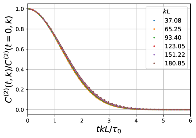
Figure 2: Time dependence of the normalized two-point correlation function $C^{(2)}(t,k)$ at different wavenumbers $k$ in the simulation at $R_{\lambda}=90$. Upper panel: data from the numerical simulation denoted with dots and its Gaussian fits denoted with continuous lines; bottom panel: the same data plotted as a function of the scaling variable $tk$, which results in the collapse of all the curves, as expected from Eq. (2). $L$ is the integral length scale, $\tau_{0}$ is the large eddy-turnover time scale.

According to the theoretical expression Eq. (2), we expect a Gaussian dependence in $t$ at small time delays, which we precisely observe in all our simulations. We show in the Fig. 2 an example of the numerical results for $C^{(2)}$ at various wavenumbers for $R_{\lambda}=90$. All curves display a Gaussian behavior, the fits are analyzed in details below. Prior to this, let us comment on the scaling. When plotted as a function of the variable $tk$, all the curves collapse onto a single Gaussian, as expected from the Eq. (2). This is illustrated in the bottom panel of Fig. 2. We emphasize that this $tk$ scaling of the correlation function is different from the $tk^{2/3}$ scaling that one would obtain from dimensional considerations based on the standard assumptions of Kolmogorov’s theory of turbulence, taking as the only relevant parameters the energy dissipation rate $\epsilon$ and the wavenumber $k$. As explained in Sec. II.2, the $tk$ scaling arises from dimensional analysis if the root-mean-square velocity $u_{RMS}\sim L/\tau_{0}$ is also included as a relevant parameter. This constitutes an explicit breaking of scale invariance, which originates in the random sweeping. $u_{RMS}$ is indeed the characteristic velocity scale of the random advection process of small-scale velocities by large vortices.

We now turn to the analysis of the Gaussian fits. The time correlation curves at various wavenumbers and various Reynolds numbers are fitted using the nonlinear least-square method (Levenberg–Marquardt algorithm), with the Gaussian fitting function: $f_{s}(t)=ce^{-(t/\tau_{s})^{2}}$ where $\tau_{s}$ and $c$ are the fitting parameters. Performing a nondimensionalization with parameter $L/\tau_{0}\approx u_{RMS}$ renders the correlation function plots at various Reynolds number comparable. The fitting range for all the data sets corresponds to the range of nondimensional variable $(tkL/\tau_{0})\in[0,2.5]$, within this range, all the correlation functions are accurately modelled by the Gaussian $f_{s}$.

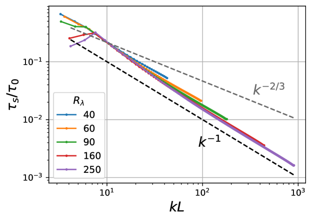
Figure 3: Dependence of the decorrelation time $\tau_{s}$ resulting from the Gaussian fit on the wavenumber in log-log scale for various $R_{\lambda}$. Times on the vertical axis are normalized by the large eddy turnover time scale $\tau_{0}$, the wavenumber on the horizontal axis is normalized by the integral length scale $L$.

The fitting parameter $\tau_{s}$ is the characteristic time scale of the correlation function, its dependence on the wavenumber $k$ is shown in Fig. 3 for various $R_{\lambda}$. While for small wavenumbers the dependence is not regular, at intermediate and large wavenumbers the decorrelation time clearly decays as $k^{-1}$. This result confirms that the collapse in the Fig. 2 occurs for the $tk$-scaling. It is also in plain agreement with a similar analysis performed in Ref. Favier, Godeferd, and Cambon, 2010.

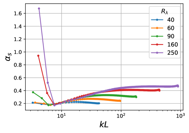
Figure 4: Estimation of the theoretical parameter $\alpha_{S}$ in the Eq. (2) from the results of the fit of numerical data.

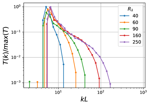
Figure 5: Rate of the direct energy transfer from the forcing range to the wavenumber $k$ normalized by the maximal value at various Reynolds numbers computed with the use of the shell-to-shell energy transfer method described in Ref. Verma, 2019.

One can estimate the coefficient $\alpha_{S}$ in the theoretical expression Eq. (2) from the fits: $\alpha_{S}\approx(\tau_{0}/\tau_{s}kL)^{2}$. Plotting $\alpha_{S}$ versus $k$ as in Fig. 4 shows that the numerical estimation of $\alpha_{S}$ reaches a plateau at large wavenumbers, which length increases with $R_{\lambda}$.

Whereas the Gaussian regime can be observed already at intermediate wavenumbers, the value of $kL$ at which $\alpha_{S}$ settles to this plateau appears to be dependent on $R_{\lambda}$. The deflection of $\alpha_{S}$ from the plateau value at the intermediate wavenumbers can be attributed to the effect of the forcing in the numerical scheme. This can be observed from the analysis of the direct energy transfers with the modes of the forcing range, as shown on the Fig. 5. The "ideal" numerical simulation would exhibit a single peak of energy transfers close to the forcing range itself, indicating the presence of the local modal interactions only, when the smaller scales receive energy only through the turbulent energy cascade. However, Fig. 5 shows that direct energy transfers occur not only in the closest vicinity of the forcing range, but also at a significant level over a band of wavenumbers, the width of which depends on $R_{\lambda}$. This means that the wavenumbers from this band are subjected not only to the local energy cascade, but also to nonlocal direct energy transfers from the forcing range. The occurrence of the nonlocal energy transfers in DNS can be a consequence of the velocity forcing concentrated in a narrow spectral band at large scales, as discussed in Ref. Kuczaj, Geurts, and McComb, 2006.

This additional non-local interaction process slows down the velocity decorrelation and results in lower values of $\alpha_{S}$. Matching the horizontal axes of the figures 4 and 5 shows that the parameter $\alpha_{S}$ reaches a constant value at wavenumbers where the direct energy exchanges with the forcing modes become negligible. We can draw from these observations that the ‘large wavenumber’ regime of the theory can be here identified as the values of $kL$ such that direct energy transfers from the forcing range are negligible.

Let us summarize this part. The data obtained from the DNS accurately confirm the theoretical expression (2) for the two-point spatio-temporal correlations of the turbulent velocity field for various scales at small time delays. In particular, the numerical data show that the theoretical parameter $\alpha_{S}$ reaches a plateau at large wavenumbers, in agreement with the theoretical result.

III.2 Three-point spatio-temporal correlations at small time delays

In this part, we estimate the three-point spatio-temporal correlations $C^{(3)}$ of the turbulent velocity field from the DNS data. The definition of $C^{(3)}$ involves a product of Fourier transforms of the velocity field $\hat{u}(t,\vec{k})$ at three different wavevectors:

$$C_{\alpha\beta\gamma}^{(3)}(t_{1},\vec{k}_{1},t_{2},\vec{k}_{2})\equiv$$

$$\left<\hat{u}_{\alpha}(t_{0}+t_{1},\vec{k}_{1})\hat{u}_{\beta}(t_{0}+t_{2},\vec{k}_{2})\hat{u}^{*}_{\gamma}(t_{0},\vec{k}_{1}+\vec{k}_{2})\right>$$ (20)

In contrast with the two-point correlation function $C^{(2)}$, the product in the expression (20) is not local in $\vec{k}$. When parallel computation and parallel memory distribution are used, the access to nonlocal quantities requires the implementation of additional communication operations between the processors during the simulation. This implies a great increase of computation time and memory. In order to avoid these additional implementation difficulties and computational costs, we study and exploit a local three-point velocity quantity naturally arising from the Navier-Stokes equation and already introduced in earlier works Kraichnan (1959).

Advection-velocity correlation function

The Navier-Stokes equation in the spectral space can be written as:

$$\partial_{t}\hat{u}_{\ell}(t,\vec{k})=\hat{N}_{\ell}(t,\vec{k})-\nu k^{2}\hat{u}_{\ell}(t,\vec{k})+\hat{f}_{\ell}(t,\vec{k})$$ (21)

where $\hat{N}_{\ell}(t,\vec{k})=-ik_{n}P_{\ell m}\sum_{k^{\prime}}\hat{u}_{m}(t,\vec{k}^{\prime})\hat{u}_{n}(t,\vec{k}-\vec{k}^{\prime})$ is the Fourier transform of the advection and pressure gradient terms of the Navier-Stokes equation, $P_{ij}=\delta_{ij}-k_{i}k_{j}/k^{2}$ is the projection tensor and $\hat{f}_{\ell}$ is the spectral forcing. Multiplying Eq. (21) by the conjugated velocity $\hat{u}^{*}_{\ell}(t_{0},\vec{k})$ at a fixed time $t_{0}$ and performing an ensemble average leads to the following equation for the two-point spatio-temporal correlation function $C^{(2)}(t,\vec{k})$:

$$(\partial_{t}+\nu k^{2})C^{(2)}(t,\vec{k})=\hat{T}(t,\vec{k})+\hat{F}(t,\vec{k})$$ (22)

where $\hat{T}(t,\vec{k})\equiv\left<\hat{N}_{i}(t+t_{0},\vec{k})\hat{u}^{*}_{i}(t_{0},\vec{k})\right>$ is the spatio-temporal correlation of the advection term and velocity, and $\hat{F}(t,\vec{k})=\left<\hat{f}_{i}(t+t_{0},\vec{k})\hat{u}^{*}_{i}(t_{0},\vec{k})\right>$ is the spatio-temporal correlation of the spectral forcing and velocity. Note that if the time delay is set to zero ($t=0$), then Eq. (22) simplifies to the equation of evolution of the average kinetic energy of a single spectral mode $E_{kin}(\vec{k})=\frac{1}{2}C^{(2)}(0,\vec{k})$. This energy splits into $\frac{1}{2}\hat{T}(0,\vec{k})$ (the average nonlinear energy transfer between modes) and $\frac{1}{2}\hat{F}(0,\vec{k})$ (the average forcing power input, which is assumed to be zero beyond the forcing range at large scales).

The advection-velocity correlation function $\hat{T}$ is a three-point statistical quantity, and its link with the three-point correlation function $C^{(3)}$ becomes clear if one develops the nonlinear term in the definition of $\hat{T}(t,\vec{k})$:

$$\hat{T}(t,\vec{k})\equiv\left<\hat{N}_{\ell}(t_{0}+t,\vec{k})\hat{u}^{*}_{\ell}(t_{0},\vec{k})\right>$$

$$=-ik_{n}P_{\ell m}\sum_{k^{\prime}}\left<\hat{u}_{m}(t+t_{0},\vec{k}^{\prime})\hat{u}_{n}(t+t_{0},\vec{k}-\vec{k}^{\prime})\hat{u}^{*}_{\ell}(t_{0},\vec{k})\right>$$

$$=-ik_{n}P_{\ell m}\sum_{k^{\prime}}C^{(3)}_{mn\ell}(t,\vec{k^{\prime}},t,\vec{k}-\vec{k}^{\prime})$$ (23)

Hence, the correlation function $\hat{T}$ actually provides a linear combination of three-point correlation functions. The theoretical prediction (6) suggests that this type of sum of $C^{(3)}$ must be Gaussian (at small times and large wavenumbers). Thus, if the theoretical prediction is valid, one would expect that the appropriately computed correlation function $\hat{T}$ is also a Gaussian of the variable $tk$:

$$\hat{T}(t,\vec{k})\sim\sum_{k^{\prime}}C^{(3)}_{mn\ell}(t,\vec{k^{\prime}},t,\vec{k}-\vec{k}^{\prime})\sim\exp\left\{-\alpha_{S}(L/\tau_{0})^{2}|\vec{k}|^{2}t^{2}\right\}$$ (24)

Another useful property of the correlation function $\hat{T}$ is its link with the two-point correlation function $C^{(2)}$. Considering a small time delay $t$, one can use the expression of the two-point correlation function $C_{s}^{(2)}(t,\vec{k})$ of Eq. (2). Inserting this result into Eq. (22) leads to an explicit expression for the function $\hat{T}$ at small time delays (and for wavenumbers outside the forcing range):

$$\hat{T}(t,\vec{k})=\nu k^{2}C^{(2)}(0,\vec{k})\left(1-\frac{2\alpha_{S}L^{2}}{\tau_{0}^{2}\nu}t\right)\exp\Big{\{}-\alpha_{S}(L/\tau_{0})^{2}k^{2}t^{2}\Big{\}}=$$

$$=\hat{D}(\vec{k})\left(1-2\alpha_{S}Re\cfrac{t}{\tau_{0}}\right)\exp\Big{\{}-\alpha_{S}(L/\tau_{0})^{2}k^{2}t^{2}\Big{\}}$$ (25)

where $\hat{D}(\vec{k})=\nu k^{2}C^{(2)}(0,\vec{k})$ is the spectral dissipation rate and $Re=\frac{U_{RMS}L}{\nu}$ is the Reynolds number. Eq. (25) indicates that the function $\hat{T}$ is in general not symmetric with respect to the origin of the $t$-axis, and that it can have a minimum and maximum at non-zero time delay $t$.

To sum up, the advection-velocity correlation function $\hat{T}$ is a local quantity in spectral space, as it implies the multiplication of the advection and velocity fields at the same wave vector $\vec{k}$, and it is related to a sum of three-point nonlocal velocity correlation functions. The equivalence of the function $\hat{T}$ at zero time delay to the spectral energy transfer function and its link with the two-point spatio-temporal correlation function Eq. (22) facilitate the testing of the numerical method and the interpretation of the results in the following. Note that an equation similar to Eq. (22) is also used in the Direct Interaction Approximation scheme (DIA) Kraichnan (1959), where a time dependent triple statistical moment similar to $\hat{T}$ is introduced.

Numerical method

In the numerical simulations, we compute the correlation function $\hat{T}(t,\vec{k})$ by point-wise multiplication of the Fourier transform of the nonlinear term $\hat{N}(t_{0}+t,\vec{k})$ by the velocity field $\hat{u}^{*}(t_{0},\vec{k})$. This quantity is local in spectral space and the computation does not require significantly more computational resources.

We use the method already described in the Sec. III.1 to collect and average the data. However, note that in this case it becomes necessary to take into account the sign of the time delay. The advection-velocity correlation function $\hat{T}$ at negative time delays can be computed just by switching the time instants of the fields in the following way:

$$\hat{T}(t,\vec{k})=\begin{cases}\left<\hat{N}_{i}(t_{0}+|t|,\vec{k})\hat{u}_{i}^{*}(t_{0},\vec{k})\right>,&t>0\\ \left<\hat{N}_{i}(t_{0},\vec{k})\hat{u}_{i}^{*}(t_{0}+|t|,\vec{k})\right>,&t<0\end{cases}$$ (26)

Hence, to compute the correlation $\hat{T}(t,\vec{k})$ at negative time delays during the simulation one only needs to store the spectral advection field at one reference time $t_{0}$.

Scale decomposition

Although the advection-velocity correlation function $\hat{T}$ provides a three-point statistical quantity that can be easily accessed in the numerical simulations, it contains a summation coming from the convolution in the advection term Eq. (23). Contributions from all possible wavevector triads $\{\vec{k}^{\prime},\vec{k}-\vec{k}^{\prime},\vec{k}\}$ of any scale are thus summed up. However, the FRG prediction Eq. (5) is valid in the limit where all three wavenumbers are large. One hence needs to refine this sum in order to eliminate contributions from the small wavenumbers.

The simplest way to solve this issue is to perform a scale decomposition of the velocity fields. We choose a threshold wavenumber $K_{c}$, so that all wavevectors of smaller norm $|\vec{k}|<K_{c}$ are considered as "large" scales and are denoted with a superscript $L$, whereas the modes with higher wavenumbers are considered as "small scales" and denoted with $S$. The velocity field is decomposed into small- and large-scale parts $\vec{u}=\vec{u}^{L}+\vec{u}^{S}$. In the spectral domain the decomposition is performed by a simple box-filtering operation:

$$\hat{u}^{L}_{i}(\vec{k},t)=\begin{cases}\hat{u}_{i}(\vec{k},t),&|\vec{k}|<K_{c}\\ 0,&|\vec{k}|\geq K_{c}\end{cases}\ \hat{u}^{S}_{i}(\vec{k},t)=\begin{cases}0,&|\vec{k}|<K_{c}\\ \hat{u}_{i}(\vec{k},t),&|\vec{k}|\geq K_{c}\\ \end{cases}$$ (27)

The velocity field scale decomposition leads to a decomposition of the advection-velocity correlation function $\hat{T}$ into four terms (here written as an example for a wavevector $\vec{k}$ belonging to the "small" scales):

$$\hat{T}(\vec{k},t)=\left[\hat{T}^{SSS}+\hat{T}^{SLS}+\hat{T}^{SSL}+\hat{T}^{SLL}\right](\vec{k},t)$$ (28)

with $\hat{T}^{XYZ}(\vec{k},t,t_{0})=-{[\hat{u}_{i}^{X}]^{*}}(\vec{k},t_{0})\ \text{FT}[u_{j}^{Y}\partial_{j}u_{i}^{Z}](\vec{k},t_{0}+t)$ where $X,Y,Z$ stand for $S\ \text{or}\ L$.

A similar decomposition at equal times has been used in studies of the energy transfer function (Ref. Frisch and Kolmogorov, 1995; Verma, 2019). Using the terminology of Ref. Verma, 2019 for energy transfers, the first superscript of a decomposition term is related to the mode receiving energy in a triadic interaction process (it is actually the mode $\vec{k}$ for which the equation (28) is written setting $t=0$), the intermediate superscript denotes the mediator mode and the last superscript is related to the giver mode that sends the energy to the receiver mode. The mediator mode does not loose nor receive energy in the interaction, it is related to the velocity field which comes as prefactor of the operator nabla in the nonlinear term of the Navier-Stokes equation, so one can term it the "advecting" field.

Let us give a physical interpretation of the terms of this decomposition. The term $\hat{T}^{SSS}$ gathers all triadic interactions where the three modes belong to the small scales. The term $\hat{T}^{SLS}$ is related to the energy transfers between two small scales mediated by large scale modes. Both energy transfers $\hat{T}^{SSS}$ and $\hat{T}^{SLS}$ occur between small scales, and are thus supposed to be local in spectral space, so they form the turbulent energy cascade. The terms $\hat{T}^{SSL}$ and $\hat{T}^{SLL}$ denote the direct energy transfers from large scale modes to small scale modes, thus non-local interactions that we expect to be small compared to the local interactions. Let us now focus on the all-small scale term $\hat{T}^{SSS}$, which corresponds to the limit of large wavenumbers on which the theoretical prediction relies.

The cut-off wavenumber $K_{c}$ of the filter in the Eq. (27) is chosen in such a way that at $k\gtrsim K_{c}$ the direct energy transfer between small scale modes and those of the forcing range (shown in the Fig. 5) becomes negligible. We expect that the dynamics of the modes at $k\gtrsim K_{c}$ does not depend directly on the forcing mechanism and we should observe an approach to the universal behavior predicted by the theory. The value of $K_{c}L$ used for each simulation is provided in Table 1. The wavenumbers $k\gtrsim K_{c}$ approximately correspond to the range of validity of the theoretical prediction for the two-point correlation function at large wavenumbers, as discussed in the Sec. III.1.

Results for the temporal correlations

The data presented in this section are obtained from the same set of simulations used for the analysis of the two-point correlation function at small time delays in Sec. III.1 and described in Table 1.

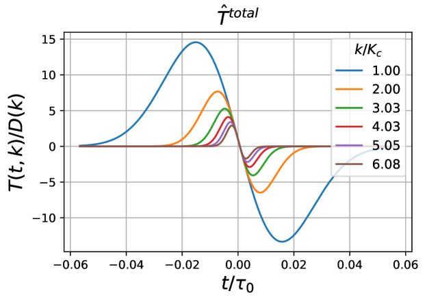
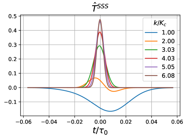
Figure 6: The advection-velocity spatio-temporal correlation function $\hat{T}(t,\vec{k})$ versus time at selected values of wavenumbers $k/K_{c}$: total one (top panel), small scale one $\hat{T}^{SSS}$ (bottom panel). The curves are normalized by the spectral dissipation rate $\hat{D}(k)=\nu k^{2}C^{(2)}(0,k)$.

The results for the time dependence of $\hat{T}$ at different wavenumbers $k\gtrsim K_{c}$ are shown in Fig. 6. One observes that the total advection-velocity correlation function $\hat{T}$ (top panel of Fig. 6) is not symmetric with respect to the time origin and takes negative values, in qualitative agreement with the form of the Eq. (25). However, the term $\hat{T}^{SSS}$, which only contains contributions from small scale modes to the correlation function $\hat{T}$, significantly changes shape (bottom panel of Fig. 6).

For the wavenumbers close to the cut-off wavenumber $K_{c}$, the curves are affected by the filter. To explain this, one should recall that at zero time delay $\hat{T}^{SSS}(t=0,\vec{k})$ is equal to the local nonlinear energy transfer between small scales modes. At wavenumbers close to the filter cut-off $K_{c}$, some spectral modes participating in the local energy transfers are suppressed by the filter. Thus, the modes close to the filter cut-off transmit the energy to smaller scales, but they do not receive energy from the nullified larger scales, which results in a negative energy balance.

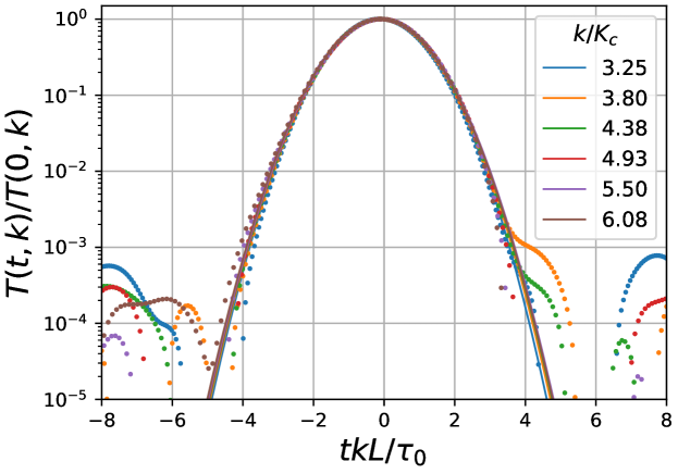
Figure 7: The small scale advection-velocity correlation function $\hat{T}^{SSS}$ versus $tk$ in semilog scale at various wavenumbers, for $R_{\lambda}=160$, $N=512$. The correlation functions are normalized by their value at $t=0$.

For the larger wavenumbers $k\gtrsim 2K_{c}$, the curves deform towards the expected Gaussian shape. This is further illustrated on Fig. 7, where the correlation function $\hat{T}^{SSS}$ is plotted versus the scaling variable $tk$ in semi logarithmic scale, inducing a collapse of all the curves onto a single Gaussian. This is in plain agreement with the theoretical result (5) for the three-point correlation function. This behavior is very similar to the one for the two-point correlation function presented in Fig. 2.

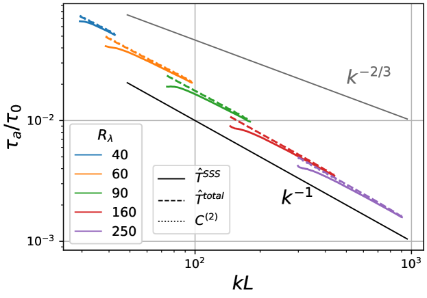
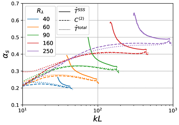
Figure 8: Numerical estimation of the parameter $\tau_{a}$ (upper panel) and $\alpha_{S}$ (bottom panel) obtained from the small scale advection-velocity correlation $\hat{T}^{SSS}$ (continuous lines), compared with the result for the two-point correlation function $C^{(2)}$ from Fig. 4 (dash-dotted lines). Both estimations converge to a similar value, as expected from the theory. The result of the fitting for the total advection-velocity correlation $\hat{T}$ is also indicated with dotted lines for completeness.

We fit the curves obtained for the advection-correlation function $\hat{T}$ with a function of the form of Eq. (25):

$$f(t)=c\left(1-\frac{t}{\tau_{b}}\right)e^{-(t/\tau_{a})^{2}}.$$ (29)

where $\tau_{a},\tau_{b}$ and $c$ are the parameters.

We find that both correlation functions $\hat{T}$ and $\hat{T}^{SSS}$ accurately fit (29). Moreover, we verify that the fitting parameter $\tau_{a}$ for both functions is proportional to $k^{-1}$, as displayed in Fig. 8 (upper panel), and in agreement with Eq. (5). We estimate from this parameter the value of the coefficient $\alpha_{S}$ in Eq. (6) as $\alpha_{S}=\tau_{0}/(\tau_{a}k^{2}L^{2})$. The result is shown in Fig. 8. At sufficiently large wavenumbers, the values of $\alpha_{S}$ extracted from the small scale function $\hat{T}^{SSS}$ and from the total $\hat{T}$ are comparable. They also match with the value obtained from $C^{(2)}$, as predicted by the theory. The small discrepancy visible between the values of $\alpha_{S}$ from $C^{(2)}$ and from $\hat{T}^{SSS}$ could be attributed to a loss of accuracy due to the decomposition: The magnitude of the filtered signal is much weaker, so it is more sensitive to the noise due to numerical errors.

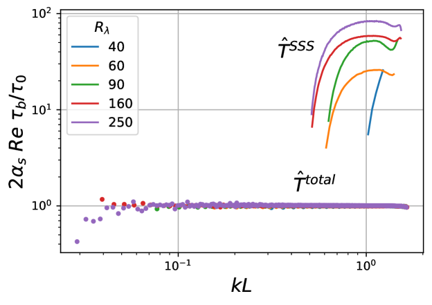
Figure 9: Dependence of the parameter $\tau_{b}$ of the fitting function Eq. (29) on the wavenumber for the small scale advection-velocity correlation $\hat{T}^{SSS}$ (continuous) and for the total one $\hat{T}$ (dotted lines). The values are normalized by $2\alpha_{s}Re/\tau_{0}$ to enable comparison with the Eq. (25).

Lastly, we examine the role of the parameter $\tau_{b}$ in the fitting function (29). To do this, we can refer to the Eq. (25) for the total correlation function $\hat{T}$, which was obtained from the Navier-Stokes equation assuming that the two-point correlation function $C^{(2)}$ has a Gaussian shape. Therefore, the fitting parameter time scale $\tau_{b}$ can be estimated as:

$$\tau_{b}=\frac{\tau_{0}}{2\alpha_{s}Re}$$ (30)

In the Fig. 9, we show the dependence of the nondimensional parameter $2\alpha_{S}Re\tau_{b}/\tau_{0}$ on the wavenumber. The values of $\alpha_{s}$ for the normalization are taken from the fit of the two-point correlation function $C^{(2)}$. As expected, for the total advection-correlation function $\hat{T}$ the values from all simulations are in the vicinity of unity independently from the wavenumber, which is consistent with the Eq. (30). Besides, one can observe from the Fig. 9 that for $\hat{T}^{SSS}$ the non-dimensionalized parameter $\tau_{b}$ is at least one order of magnitude larger than for the total $\hat{T}$. This means that for $\hat{T}^{SSS}$ the time scale of the linear part $\tau_{b}$ of the function (29) becomes much larger than the time scale $\tau_{a}$ of the Gaussian part. In other words, the Gaussian part decays fast and the function already approaches zero before the slower linear part comes into play, which results in the Gaussian-like shapes of $\hat{T}^{SSS}$ in the figures 6 and 7. On the contrary, for the total function $\hat{T}$ the time scale $\tau_{b}$ is smaller than $\tau_{a}$ and the shape of the total $\hat{T}$ is dominated by the linear part at short times, resulting in a non-symmetric shape.

An interpretation of this result can be proposed based on the identification of the advection-velocity correlation function $\hat{T}$ at $t=0$ as the spectral energy transfer function. We have observed that a significant part of the energy transfers between the small scales in 3D turbulence occurs in spectral triads with participation of a large scale mode as mediator (the term $\hat{T}^{SLS}$ in the decomposition (28)). The same conclusion can be found in Ref. Verma, 2019; Domaradzki and Rogallo, 1990; Ohkitani and Kida, 1992. However, as discussed in Ref. Aluie and Eyink, 2009, although these triads have significant individual contributions to energy transfer, they are much less numerous than the fully local triads formed of small-scale modes (the term $\hat{T}^{SSS}$ in the decomposition), because there are fewer large-scale modes. In the limit of large Reynolds numbers, the fully local triads become numerous and dominate in the turbulent energy cascade.

In addition, the detailed analysis of the contributions in the decomposition (28) shows that the nonsymmetric behavior in time of the total correlation $\hat{T}$ is also determined by the contribution of $\hat{T}^{SLS}$. The occurence of the maximal and minimal values of the advection-velocity correlation $\hat{T}$ at non-zero time delays (see the top panel of the Fig. 6) implies that there is some coherence between two small scale vortices simultaneously advected by a large scale, slowly varying, vortex. The origin of this coherence can be through an alignment of turbulent stress and large scale strain rate. The dynamics of the alignment between time-delayed filtered strain rate and the stress tensors, as well as its link with the energy flux between scales, has been recently analyzed in the Ref. Ballouz, Johnson, and Ouellette, 2020, where the alignment also displays an asymmetrical behavior in time and is peaked at scale dependent time delays. As the energy flux, which could be expressed as a product of stress and strain rate, also represents a triple statistical moment of the velocity field, it would be natural to expect that it exhibits a temporal behavior similar to the advection-velocity correlation $\hat{T}$.

In the case of the purely small scale correlation function $\hat{T}^{SSS}$, the characteristic time scales of all modes in the triad are comparable, and the mediator mode cannot impose any coherence on the interacting modes, as all three modes decorrelate faster before any alignment could occur. This results in the symmetric, close to Gaussian form of the small scale correlation functions $\hat{T}^{SSS}$. Note that all the three modes in $\hat{T}^{SSS}$ are still transported simultaneously by the random large scale velocity field. This mechanism is the same random sweeping effect that is reponsible for the Gaussian time dependence of $\hat{T}^{SSS}$ and of $C^{(2)}$.

To conclude, the spatio-temporal correlation between the velocity and advection fields constitutes a triple statistical moment easily accessible in numerical simulations. The application of the scale decomposition to this correlation is a necessary refinement to approach the regime of large wavenumbers of the theoretical result and gives an insight into the statistics of the three-point spatio-temporal correlation functions. We observe a Gaussian with the same time and wavenumber dependence as in the theoretical prediction. Moreover, this analysis provides also a nontrivial validation of the theoretical result, which predicts the parameter $\alpha_{S}$ to be the same for the two-point and the three-point correlations.

III.3 Two-point spatio-temporal correlation of the modulus of the velocity

The numerical analysis of the two-point correlation function at large time delays represents a more challenging task, as the values of the correlation functions become very low and are drowned into noise and numerical errors. Moreover, it requires larger observation times, and thus longer simulations and more computational resources. We did not succeed in resolving the large time regime from our numerical data for the two-point correlation function, due to both the lack of statistics in the time averaging and the weakness of the signal, comparable with numerical errors.

However, in order to increase the amplitude of the signal, we study the correlation function of the velocity modulus rather than the real part of the complex correlation function. For this quantity, the large time regime indeed turns out to be observable, as we now report. We thus introduce the connected two-point correlation function of velocity modulus in spectral space

$$\bar{C}_{n}^{(2)}(t,k)=\left<\lVert\hat{\vec{u}}({t_{0}},\vec{k})\rVert\ \lVert\hat{\vec{u}}({t_{0}}+t,\vec{k})\rVert\right>-$$

$$\left<\lVert\hat{\vec{u}}({t_{0}},\vec{k})\rVert\right>\left<\lVert\hat{\vec{u}}({t_{0}}+t,\vec{k})\rVert\right>$$ (31)

with spatial and time averaging identical to Eq. (18) $\left<...\right>=\frac{1}{N_{t}}\frac{1}{M_{n}}\sum_{j=1}^{N_{t}}\sum_{\vec{k}\in S_{n}}(...)$. This correlation function was computed in another set of simulations with larger width of the time window.

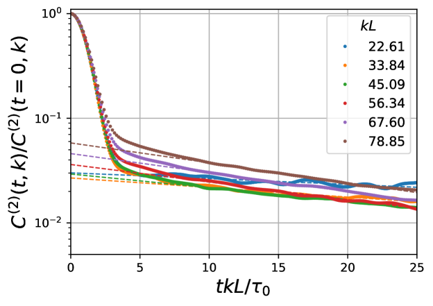
Figure 10: Time dependence of the normalized two-point correlation function of the velocity norms $\bar{C}_{n}^{(2)}(t,k)$ at $R_{\lambda}=60$ for different wavenumbers $k$ in semi-logarithmic scaling. The numerical data are denoted with dots, the exponential fit is denoted with the dashed lines.

An example of the correlation function computed according to Eq. (31) for $R_{\lambda}=60$ is presented in Fig. 10. Similarly to the two-point correlation studied in Sec. III.1, one observes at short time delays the Gaussian decay in time and the curves at different wavenumbers collapse in the $tk$-scaling. However, Fig. 10 reveals a crossover to another regime at larger time delays: a slower decorrelation in time, that can visually be estimated as exponential. The curves at various wavenumbers do not collapse anymore in the horizontal scaling $tk$, and the slope of the correlation function appears to be steeper for larger wavenumbers.

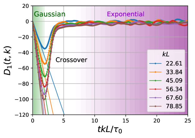
Figure 11: The normalized time derivative $D_{1}$ defined in Eq. (32) calculated numerically with the data from the simulation at $R_{\lambda}=60$. The linear part of $D_{1}$, highlighted by green shades, corresponds to the Gaussian decay at small time delays, and the approximately constant part of $D_{1}$, highlighted by purple shades, corresponds to the exponential time correlation at large time delays.

We compute the normalized time derivative of $\bar{C}_{n}^{(2)}(t,k)$ in order to study the transition between the two time regimes of the correlation function:

$$D_{1}(t,k)=\frac{\partial_{t}{\bar{C}_{n}^{(2)}}(t,k)}{\bar{C}_{n}^{(2)}(t,k)}.$$ (32)

If the correlation function $\bar{C}_{n}^{(2)}$ is a Gaussian, the time derivative $D_{1}$ is simply a line with a slope equal to $-2/{\tau_{s}^{2}}$, and if the correlation function is an exponential function, the function $D_{1}$ becomes a constant. The derivative $D_{1}$ is represented in Fig. 11 for $R_{\lambda}=60$. At small time delays, $D_{1}$ is a linear function with a negative slope. It then displays a non-monotonous transition before approximately reaching a constant value at large time delays. We can define the crossover time delay $t$ as the location of the minimum of the derivative $D_{1}$. This crossover time at different Reynolds numbers is shown in the Fig. 12. It depends on the wavenumber as $\tau_{c}\sim k^{-1}$. We checked that this $k^{-1}$ behavior does not depend on the precise definition chosen for the crossover time.

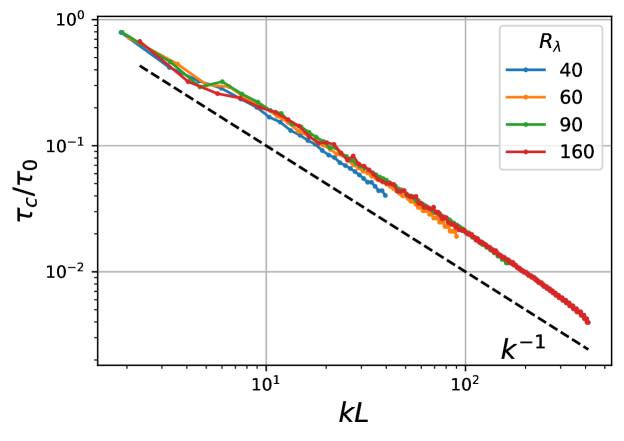
Figure 12: Crossover time for the two-point correlations of the velocity norms $\bar{C}^{(2)}_{n}$ between the small time and large time regimes as a function of the wavenumber $k$, estimated from the minimum of $D_{1}$.

Let us emphasize that the correlation function of the velocity norms introduced in Eq. (31) is not related in any simple way to the standard real part of the correlation function (1) computed theoretically in the FRG approach. Moreover, as the phases play no role for these correlations, the sweeping argument proposed in Sec. II.2 cannot explain this behavior. The decorrelation must ensue a priori from another physical mechanism, yet to be identified. However, the results of the numerical simulation show that the correlation of the velocity modulus and the real part of the complex velocity correlation function at small time delays (the Gaussian decay) are similar, and exhibit close values for the characteristic decorrelation time. In addition, at large time delays the correlations of the velocity modulus demonstrate a crossover to an exponential decay in time, analogous to the one expected for the real part of the correlation function.

While a complete understanding of these intriguing observations is lacking, some insight into the mechanisms at play in the regime of small time delays can be obtained from the expression valid to first-order in $t$

$$\vec{u}({t_{0}}+t,\vec{r})=\vec{u}({t_{0}},\vec{r}-\vec{u}({t_{0}},\vec{r})t)-\vec{\nabla}p({t_{0}},\vec{r})t+{\cal O}(t^{2}),$$

where the second term which is required to enforce incompressibility involves the pressure satisfying the Poisson equation $-\triangle p({t_{0}},\vec{r})={\rm tr}[(\vec{\nabla}\vec{u}({t_{0}},\vec{r}))^{2}].$ If one assumes that the $\vec{r}$-dependence can be ignored for the inner velocity field multiplied by $t,$ then this expression simplifies to

$$\vec{u}({t_{0}}+t,\vec{r})=\vec{u}({t_{0}},\vec{r}-\vec{u}({t_{0}},\vec{0})t)+{\cal O}(t^{2})$$

and one obtains $\hat{\vec{u}}({t_{0}}+t,\vec{k})=e^{-it\vec{k}\cdot\vec{u}({t_{0}},\vec{0})t}\hat{\vec{u}}({t_{0}},\vec{k}),$ so that sweeping is represented by a pure change of phase of the Fourier mode. However, it is clearly inconsistent to neglect the $\vec{r}$-dependence of $\vec{u}({t_{0}},\vec{r})$ in one instance and not in the other. Thus, the effects observed in Fig. 11 must presumably be due to the spatial inhomogeneity of sweeping and the associated long-range pressure forces arising from incompressibility, which decorrelate the moduli of the Fourier velocity amplitudes. If one furthermore plausibly assumes that the correlation $\bar{C}_{n}^{(2)}(t,k)$ is a maximum at $t=0$, then analyticity in $t$ requires in the regime of small time delays that $\bar{C}_{n}^{(2)}(t,k)\doteq\bar{C}_{n}^{(2)}(0,k)(1-t^{2}/\tau^{2}_{k})$ for some parameter $\tau_{k}$ with units of time and then immediately

$$D_{1}(t,k)\doteq 1-\frac{2t}{\tau^{2}_{k}},$$

as observed in Fig 11. These considerations do not explain the detailed observations, neither the $k$-dependence of $\tau_{k}$ nor the exponential decay in the regime of long time lags, but they do suggest some possible relevant physics for future theoretical and empirical exploration.

Interestingly, a very similar behavior has been observed in the air jet experiments described in Ref. Poulain et al., 2006. In these experiments, the temporal decay of the two-point correlation function of the amplitude of the vorticity field is measured, and it displays a crossover from a $tk$ Gaussian decay to a slower exponential one. The crossover time between these two regimes is found to scale as $k^{-1}$ as observed in our simulations Baudet (2020).

IV Summary and Perspective

In this paper, we use DNS to study the spatio-temporal dependence of two-point and three-point correlations of the velocity field in stationary, homogeneous and isotropic turbulence. The motivation underlying this work is to test a theoretical result obtained within the FRG framework, which gives the exact leading term at large wavenumbers of the spatio-temporal dependence of any $n$-point correlation function of the velocity field Tarpin, Canet, and Wschebor (2018). This result establishes that the two-point correlation function decays as a Gaussian in the variable $tk$ (or $|\sum_{i}t_{i}\vec{k_{i}}|$ for a $n$-point correlation) at small time delays $t_{i}$, while at large time delays, the decorrelation slows down to a simple exponential in $t_{i}$. While these results can in fact be interpreted quite simply by extending the analysis of the random sweeping effect, following the original arguments by Kraichnan, they are endowed through the FRG calculation with a rigorous and very general expression. In particular, these expressions show that for any fixed time delays, the correlation function as a function of any wavenumber is always Gaussian. Furthermore, the multiplicative constant in the exponential is the same for all the Gaussian decays and all the exponential decays as well, independently from the order $n$.

In the small time regime that we could access via DNS of the two-point and three-point correlation functions with an equal time delay, our numerical data confirm the theoretical prediction with great accuracy. In particular, we verify that the prefactors of time are proportional to $k^{2}$ (or $|\vec{k}_{1}+\vec{k}_{2}|^{2}$) and the numerical constants at small time delays are indeed equal for the two-point and three-point correlations. Furthermore, our analysis provides a deeper insight into the range of validity of the theory. All the theoretical results discussed here are derived under the assumption that all the wavenumbers (and their partial sums) are large. From the DNS data, we estimate the range of $k$ where this condition is fulfilled and show that it corresponds to the range where the direct energy transfer from the forcing modes is negligible. For the three-point correlations, we show that once the small wavenumbers $k<K_{c}$ are removed through an appropriate decomposition, the theoretical prediction is precisely recovered.

Our analysis of the correlation function of the modulus of the velocity shows a very similar behavior as the one expected for the velocity itself, although the theoretical results do not apply in this case. It would be desirable to understand the main physical mechanism at play for the decorrelation of the modulus, which cannot be attributed to convective dephasing. This calls for further theoretical developments. On the numerical side, it would be interesting to extend this analysis to higher-order correlations, and for more general configurations in time (since our approach restricts to equal and short time delays for the three-point correlations). A particularly challenging task is the access to the long-time regime. This would of course require important computing resources. The understanding of the temporal correlations for passive scalars in turbulent flows is also very important for many applications. This is work in progress.