Machine Learning for Auxiliary Sources

Abstract

We rewrite the numerical ansatz of the Method of Auxiliary Sources (MAS), typically used in computational electromagnetics, as a neural network, i.e. as a composed function of linear and activation layers. MAS is a numerical method for Partial Differential Equations (PDEs) that employs point sources, which are also exact solutions of the considered PDE, as radial basis functions to match a given boundary condition. In the framework of neural networks we rely on optimization algorithms such as Adam to train MAS and find both its optimal coefficients and positions of the central singularities of the sources. In this work we also show that the MAS ansatz trained as a neural network can be used, in the case of an unknown function with a central singularity, to detect the position of such singularity.

1 Introduction

Computational electromagnetics studies how to numerically solve Maxwell’s boundary value problems for engineering and scientific applications. An example is the simulation of plasmonic nanoparticles, which can exhibit an interesting behavior (such as scattering) with electromagnetic radiation at a wavelength far larger than the particle size, depending on, e.g., the particle geometry (Koch et al., 2018). This phenomenon is relevant for many applications, such as solar cells or cancer treatment.

For this kind of problems, several numerical methods have been developed based on a partition of the geometric domain: for example, the finite-difference time-domain method (Yee, 1966), using a regular grid, or the Finite Element Method (FEM) for frequency-domain Maxwell’s equations (Hiptmair, 2002), using an unstructured mesh typically made of triangles (2D) or tetrahedra (3D). These approaches employ basis functions locally supported on the entities of the partition and therefore lead to large, sparse linear systems to solve.

Conversely, another line of research in computational electromagnetics involves methods that do not need a mesh, as they make use of global basis functions (nonzero everywhere) that are exact solutions of the Partial Differential Equation (PDE) of interest. Given their nature, these basis functions do not need to be as many as the elements of FEM to achieve a good approximation, but, as we will see in a moment, require additional care. The numerical solution here is obtained by matching on a hypersurface either a boundary condition or interface conditions with another domain, discretized by 1) different basis functions, as the PDE may be different there, or 2) an entirely other method (Casati & Hiptmair, 2019).

More details on these so-called Trefftz methods (Hiptmair et al., 2016) are given in the next section. Here it suffices to say that a common choice of Trefftz basis functions are point sources, i.e. exact solutions that exhibit a central singularity. The centers of these singularities are placed in the complement of the respective domain of approximation, so that they are ignored by the computations.

Furthermore, one would like to position these singularities in a way that the unknown function is well approximated by a linear combination of the sources. This holds true even if it can be proven that Trefftz methods enjoy exponential convergence when the unknown function has an analytic continuation beyond its approximation domain (Casati & Hiptmair, 2019): as an example, please refer to the results in table 1 below. In a way, the goal here is similar to choosing a high-quality unstructured mesh for FEM (Brenner & Scott, 2008) before assemblying and solving the related linear system.

To find this “optimal” positioning of the sources, the state-of-the-art is based on elaborate heuristic rules developed over the years to support the user’s manual positioning, especially in the context of computational electromagnetics, where one Trefftz method is the Multiple Multipole Program (MMP) (Hafner, 1999). These heuristic rules are based on the curvature radius (Moreno et al., ) or on an unstructured surface mesh (Koch et al., 2018) of the hypersurface where the boundary condition needs to be imposed. Another line of research made use of genetic algorithms (Heretakis et al., 2005).

Here we propose an approach based on an optimization algorithm usually employed to train neural networks. As a numerical example for validation, let us consider for simplicity a Poisson’s problem in a 2D bounded domain $\Omega$ – in computational electromagnetics it can model, e.g., a vector magnetic potential orthogonal to the 2D plane – with a manufactured solution of the type

$$\rho_{x\sigma}^{-1}\sin(\theta_{x\sigma}){\color[rgb]{0,0,0},}$$ (1)

expressed in polar coordinates ($r\in[0,\infty)$, $\theta\in[0,2\pi)$) of ${\mathbf{x}}_{\sigma}\coloneqq{\mathbf{x}}-\bm{\sigma}$, with ${\mathbf{x}},\bm{\sigma}\in\mathbb{R}^{2}$ position vectors in Cartesian coordinates. Specifically, the center $\bm{\sigma}$ is taken in $\mathbb{R}^{2}\setminus\Omega$.

Let us then approximate this problem with 3 point sources, randomly placed in $\mathbb{R}^{2}\setminus\Omega$ not too far from the hypersurface $\Gamma\coloneqq\partial\Omega$, and obtain their coefficients in a least-squares sense by matching the values of 1 on selected points of $\Gamma$.

Table 1: Relative $L^{2}(\Omega)$-error of 3 point sources to approximate 1 for 10 different centers $\bm{\sigma}$ before and after the optimization ($5\cdot 10^{5}$ epochs).

Initial      positions	After      algorithm
51.19%	1.32%
32.07%	1.09%
44.83%	1.01%
10.70%	0.85%
78.28%	0.94%
15.37%	2.40%
28.23%	1.26%
32.15%	3.63%
10.11%	1.29%

Table 1 presents the corresponding $L^{2}(\Omega)$-error (given a bounded $\Omega$) of this ansatz with respect to 1, considering 10 different random centers $\bm{\sigma}$ not too far from $\Gamma$. The first column lists the relative errors (with respect to the $L^{2}(\Omega)$-norm of 1) for this random placement of the sources, which are as high as 78.28%. Conversely, as shown by the errors in the second column, placing the sources with the optimization algorithm proposed in this work allows to achieve a better approximation with the same ansatz.

1.1 Summary and Structure

Compared to the state-of-the-art of Trefftz methods, by using the approach proposed in this paper we claim

• a higher accuracy, as shown by the results of table 1, which can also improve the more epochs are considered for the optimization,

• at a low additional runtime, given the efficient implementations of the optimization algorithms for neural networks: it takes a matter of seconds for the $5\cdot 10^{5}$ epochs of table 1.

• This is also supported by the fact that the centers of the sources form a limited quantity of additional degrees of freedom for the optimization algorithm (on top of the coefficients of the sources). In fact, their number is not high (typically of an order of magnitude of 2) because of the exponential convergence of Trefftz methods. This allows to handle large system sizes for real-world engineering applications without particular restrictions.

The work is organized as follows: after this introduction, the fundamentals of Trefftz methods, specifically of MMP, are presented in Section 2. Next, details on how to use the optimization algorithms of neural networks for MMP are given in Section 3. This approach is then supported by the numerical results presented in Section 4. Finally, Section 5 concludes the paper.

2 Trefftz Methods

Trefftz methods employ exact solutions of the PDE as (global) basis functions. Hence, the main feature that characterizes a Trefftz method is its own discrete function space. As an example, for a 2D homogeneous Poisson’s problem on a bounded domain $\Omega$, we work with the continuous Trefftz space of functions

$$\mathcal{T}(\Omega)\coloneqq\Big{\{}f\in H_{\text{loc}}^{1}(\Omega)\!:\>\nabla^{2}v=0\Big{\}}{\color[rgb]{0,0,0}.}$$ (2)

The functional form of the corresponding discrete basis functions leads to different types of Trefftz methods:

• Plane waves (Griffiths, 2013) or (generalized) harmonic polynomials (Moiola, 2011) constitute the most common choice (Hiptmair et al., 2016).

• If Trefftz basis functions solve an inhomogeneous problem, then we obtain the method of fundamental solutions (Kupradze & Aleksidze, 1964).

• Conversely, if they are point sources solving homogeneous equations (the right-hand side can be expressed by a known offset function), we get the Method of Auxiliary Sources (MAS) (Zaridze et al., 2000).

Concretely, from now on let us focus on a special case of MAS, i.e. the Multiple Multipole Program already introduced in Section 1.

The concept of this method was proposed by Ch. Hafner in his dissertation (Hafner, 1980) and popularized by his free code OpenMaXwell (Hafner, 1999) for 2D axisymmetric problems based on Maxwell’s equations, especially in the fields of photonics and plasmonics. Hafner’s MMP is in turn based on the much older work of G. Mie and I. N. Vekua (Mie, 1900; Vekua, 1967). Essentially, the Mie–Vekua approach expands some scalar field in a 2D multiply-connected domain (Gamelin, 2001) by a multipole expansion supplemented with generalized harmonic polynomials. Extending these ideas, MMP introduces more basis functions (multiple multipoles) than required according to Vekua’s theory (Vekua, 1967) to span the Trefftz spaces 2.

More specifically, multipoles are potentials spawned by (anisotropic) point sources. These point sources are taken from the exact solutions of the homogeneous PDE, here Laplace’s equation, which are subject to a condition at infinity when they are used to approximate the solution in an unbounded domain.

A multipole can generally be written as $f({\mathbf{x}})\coloneqq g(\rho_{xc})\,h(\theta_{xc})$ or ${\mathbf{f}}({\mathbf{x}})\coloneqq g(\rho_{xc})\,{\mathbf{h}}(\theta_{xc},\varphi_{xc})$ in a polar/spherical coordinate system for ${\mathbf{x}}\in\mathbb{R}^{d}$, $d=2,3$ ($r\in[0,\infty)$, $\theta\in[0,2\pi)$, $\varphi\in[0,\pi]$) with respect to its center ${\mathbf{c}}\in\mathbb{R}^{d}$ (${\mathbf{x}},{\mathbf{c}}$ are position vectors in Cartesian coordinates). Here, $\left(\rho_{xc},\theta_{xc}\right)^{\top}$ and $\left(\rho_{xc},\theta_{xc},\varphi_{xc}\right)^{\top}$ are polar/spherical coordinates of the vector ${\mathbf{x}}_{c}\coloneqq{\mathbf{x}}-{\mathbf{c}}$.

The radial dependence $g(\rho_{xc})$ has a center that presents a singularity, $\left|{g(\rho)}\right|\to\infty$ for $\rho\to 0$, and, possibly, the desired condition at infinity. Given the central singularity, multipoles are centered outside the domain in which they are used for approximation.

On the other hand, the polar/spherical dependence $h$ or ${\mathbf{h}}$ is usually formulated in terms of trigonometric functions (Abramowitz & Stegun, 1964) or (vector) spherical harmonics (Carrascal et al., 1991).

For the 2D Poisson’s problem introduced in Section 1, multipoles can have the form

$$\left(r,\theta\right)\mapsto\left\{\begin{aligned} &\log\rho_{xc},&&\\ &\rho_{xc}^{-j}\cos(j\theta_{xc}),&j&=1,\dots,\infty,\\ &\rho_{xc}^{-j}\sin(j\theta_{xc}),&j&=1,\dots,\infty,\end{aligned}\right.$$ (3)

which also satisfy the condition at infinity

$$c\log\lVert{\mathbf{x}}\rVert+\mathcal{O}(\lVert{\mathbf{x}}\rVert^{-1}),\quad c\in\mathbb{R}{\color[rgb]{0,0,0}.}$$ (4)

Figure 1 shows three examples of multipoles according to 3 with center ${\mathbf{c}}=\mathbf{0}$.

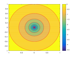
(a) $\log\rho$

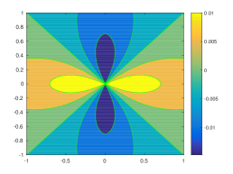
(b) $\rho^{-2}\cos(2\theta)$

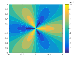
(c) $\rho^{-3}\cos(3\theta)$

Figure 1: Sample multipoles according to 3, i.e. discrete basis functions of the MMP Trefftz space 2.

Each multipole from 3 is characterized by a location, i.e. its center ${\mathbf{c}}$, and the parameter $j$ (its degree), which can be assumed 0 for the case $\log\rho_{xc}$. When we place several multipoles at a given location up to a certain order $p$, which is the maximum degree of multipoles with that center, we use the term multipole expansion. Summing the number of terms of all multipole expansions used for approximation (each with a different center) yields the total number of degrees of freedom of the discretized Trefftz space $\mathcal{T}^{n}(\Omega)$ from 2.

Once a discrete basis of multipoles has been chosen, there are several ways to find their coefficients such that the error with the boundary condition is minimized (Hiptmair et al., 2016): the most common is arguably collocation on selected matching points of the hypersurface (Hafner, 1980), which aims at minimizing the $\ell^{2}$-error at the matching points in a least-squares sense.

In this work we propose to use a gradient-based optimization algorithm, typically employed to train neural networks that have many degrees of freedom, to optimize with respect to both the coefficients of the multipoles and the centers of their singularities. In other words, we do not preselect the centers and then find the corresponding optimal coefficients, in a similar way to precomputing a finite-element mesh, but we optimize both at the same time. This is doable because the number of centers scales logarithmically with respect to the number of matching points used for collocation, considering the exponential convergence of MMP (Casati & Hiptmair, 2019).

3 MMP as a Neural Network

In this section we rewrite the numerical ansatz of MMP as a neural network, i.e. as a composed function of linear and activation layers. In this way, we are able to rely on efficient implementations of popular optimization algorithms for neural networks, such as the Adam algorithm (Kingma & Ba, 2015), as well as the automatic differentiation (Rall, 1981) component of these implementations.

The MMP ansatz approximates an unknown function as follows:

$$\sum\limits_{i=1}^{n}\sum\limits_{j=0}^{p_{i}}w_{ij}f_{ij}({\mathbf{x}}-{\mathbf{c}}_{i}){\color[rgb]{0,0,0},}$$ (5)

where

• $n$ is the number of multipole expansions,

• $p_{i}$ is the order of the $i$-th multipole expansion, i.e. we consider terms in 3 from $j=0$ (corresponding to $\log\rho_{xc}$) to $p_{i}$, and

• $w_{ij}\in\mathbb{R}$ is the coefficient of $f_{ij}({\mathbf{x}}-{\mathbf{c}}_{i})\in\mathcal{T}^{n}(\Omega)$, with ${\mathbf{x}},{\mathbf{c}}_{i}\in\mathbb{R}^{2}$ and ${\mathbf{c}}_{i}$ center of the $i$-th multipole expansion.

Following the formalism of neural networks (Haykin, 2008), we can rewrite 5 as a 3-layer neural network, given ${\mathbf{x}}\in\mathbb{R}^{2}$ as the input variable:

1. The first linear layer is represented by the following affine transformation with a nonzero shift:

   $${\mathbf{x}}\mapsto\begin{pmatrix}\left.\begin{array}[]{c}{\mathbf{I}}_{2,2}\\ \vdots\\ {\mathbf{I}}_{2,2}\end{array}\right\}p_{1}\\ \vdots\\ \left.\begin{array}[]{c}{\mathbf{I}}_{2,2}\\ \vdots\\ {\mathbf{I}}_{2,2}\end{array}\right\}p_{n}\end{pmatrix}{\mathbf{x}}-\begin{pmatrix}\left.\begin{array}[]{c}{\mathbf{c}}_{1}\\ \vdots\\ {\mathbf{c}}_{1}\end{array}\right\}p_{1}\\ \vdots\\ \left.\begin{array}[]{c}{\mathbf{c}}_{n}\\ \vdots\\ {\mathbf{c}}_{n}\end{array}\right\}p_{n}\end{pmatrix}={\mathbf{u}}\in\mathbb{R}^{2m}{\color[rgb]{0,0,0},}$$ (6)

   where $m\coloneqq\sum_{i=1}^{n}(p_{i}+1)$ and the shift (bias) is made of the centers of the multipoles, to be determined by the optimization.

2. The activation layer is composed of several “many-to-one” activation functions, as they map pairs of variables to a single one:

   $${\mathbf{f}}({\mathbf{u}})={\mathbf{v}}\in\mathbb{R}^{m}{\color[rgb]{0,0,0},}$$ (7)

   where each activation function $f_{ij}:\mathbb{R}^{2}\to\mathbb{R}$, $j=0,\dots,p_{i}$, $i=1,\dots,n$, is a multipole. Examples of “many-to-one” activation functions from the literature of neural networks include softmax, max pooling, maxout, and gating (Ramachandran et al., 2017).

3. Finally, the third layer is linear without bias:

   $${\mathbf{w}}^{\top}\cdot{\mathbf{v}}=y\in\mathbb{R}{\color[rgb]{0,0,0},}$$ (8)

   where the weights ${\mathbf{w}}\in\mathbb{R}^{m}$ are the coefficients of the multipole expansions.

Figure 2 schematizes the neural network representation of the MMP ansatz described above.

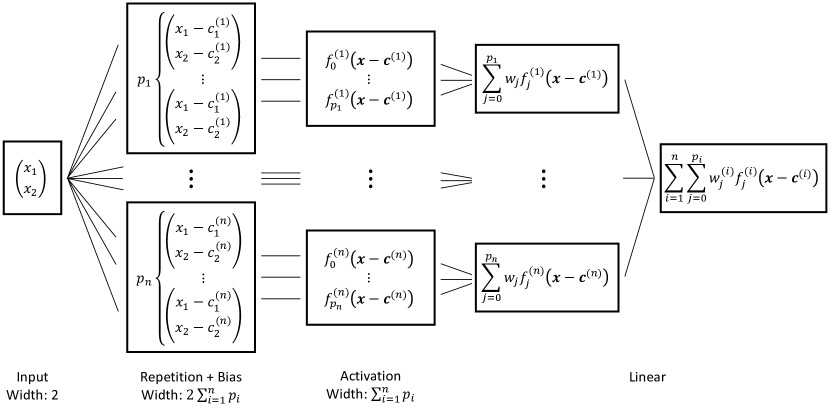
Figure 2: Neural network representation of the MMP ansatz.

Based on this representation, one can see that the centers of singularities ${\mathbf{c}}_{i}$, $i=1,\dots,n$, are, together with the coefficients $w_{ij}$, $j=0,\dots,p_{i}$, degrees of freedom of this neural network. The total number of degrees of freedom is $2n+\sum_{i=1}^{n}(p_{i}+1)$: note that, in case of few high-order multipole expansions, the additional degrees of freedom constituted by their centers ($2n$) do not have much impact on the total number.

For the loss function of this neural network we follow the collocation method, whose goal is to minimize the $\ell^{2}(\Gamma)$-error between the MMP ansatz 5 and the boundary condition on the chosen matching points:

$$L({\mathbf{c}},{\mathbf{w}})\coloneqq\sum\limits_{l=1}^{N}\left[\sum\limits_{i=1}^{n}\sum\limits_{j=0}^{p_{i}}w_{ij}f_{ij}({\mathbf{x}}_{l}-{\mathbf{c}}_{i})-y_{l}\right]^{2}{\color[rgb]{0,0,0},}$$ (9)

where $y_{l}$, $l=1,\dots,N$, are the evaluations of the unknown (assuming a Dirichlet boundary condition) on the $N$ matching points ${\mathbf{x}}_{l}$.

4 Numerical Results

As bounded domain $\Omega$ for a 2D Poisson’s problem we choose the interior region of a flower-shaped curve $\Gamma\coloneqq\partial\Omega$, parameterized by the formula

$$\left(R(\theta)\cos\theta,R(\theta)\sin\theta\right)^{\top},\quad R(\theta)=\alpha(\beta+\gamma\cos(K\theta))$$ (10)

in Cartesian coordinates, with $\theta\in[0,2\pi)$, $\alpha,\beta,\gamma\in\mathbb{R}$, and $K\in\mathbb{N}$. We set $\alpha=0.5$, $\beta=1$, $\gamma=0.5$, and $K=5$, and choose $N=100$ points of $\Gamma$ from equidistant values of $\theta\in[0,2\pi)$ to serve as matching points.

Figure 3a shows the flower-shaped curve according to 10, Figure 3b the meshed domain with triangles. This mesh is used to compute the $L^{2}(\Omega)$-error of the MMP approximation with respect to manufactured solutions of type 1 (see Section 1) with different centers $\bm{\sigma}\in\mathbb{R}^{2}\setminus\Omega$. For the numerical quadrature of the error, we employ the Gaussian quadrature rule of order 5 (polynomials up to the 5-th order are integrated exactly) on triangles.

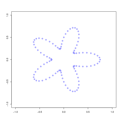
(a) Flower-shaped curve according to 10 (100 matching points).

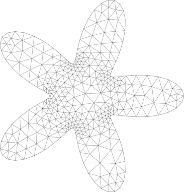
(b) Sample mesh of the flower-shaped domain.

Figure 3: Flower-shaped curve and sample mesh.

In the following we discuss two experiments solving this boundary value problem with MMP: first, we investigate the dependence of the Adam optimization on the number of multipole expansions used for approximation (Section 4.1), then on the order of a single multipole expansion (Section 4.2).

4.1 Dependence on the number of multipole expansions

With the Adam algorithm we find the coefficients and centers of singularities of the MMP expansions that minimize the boundary $\ell^{2}(\Gamma)$-error with a manufactured solution on selected matching points. The “dataset” to train the MMP ansatz as a neural network is made of coordinates of matching points as input observations and the corresponding evaluations of the manufactured solution as output.

To approximate 1, we choose an MMP ansatz made of several multipole expansions (we vary their number $n$), each of order 1. Before the Adam optimization, their centers are initially disposed on the unit circle, which is external to the bounded domain $\Omega$ of Figure 3 (see Figure 4a). The corresponding initial values for the multipole coefficients are obtained from the collocation method, given these centers.

The Adam algorithm is then run for a number of epochs until the training loss becomes smaller than 0.05, for at most $5\cdot 10^{5}$ epochs. The learning rate is 0.1 and the batch size is the full dataset (100 matching points): this is justified because the number of observations is equal to the number of matching points, set by the user, which must therefore be humanely manageable (here 100).

We perform this procedure for 100 manufactured solutions, each centered on an equidistant point of the curve 10 with parameters $\alpha=0.8$, $\beta=1$, $\gamma=0.2$, and $K=5$ (see Figure 4b).

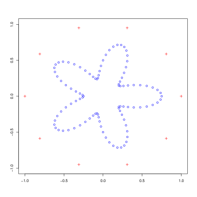
(a) In red, 10 initial centers of multipole expansions.

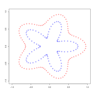
(b) In red, 100 centers of manufactured solutions.

Figure 4: Initial centers of multipoles and centers of manufactured solutions.

Figure 5 shows the $L^{2}(\Omega)$-error (normalized with the $L^{2}(\Omega)$-norm of the manufactured solution) produced by the initial positioning on the unit circle (see Figure 4a) and after the Adam optimization. The number of multipole expansions is in the range $[3,9]$ to investigate its impact on the optimization result.

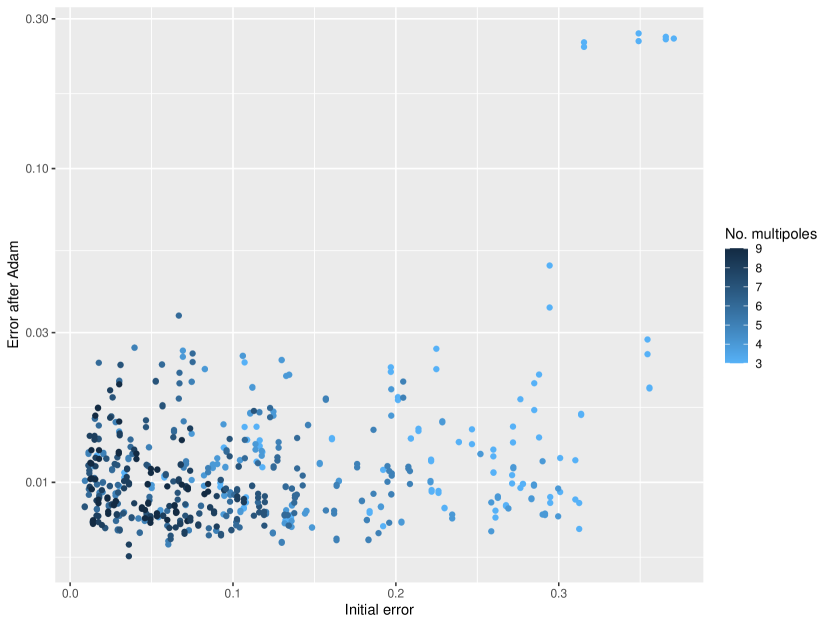
Figure 5: $L^{2}(\Omega)$-error before and after the Adam optimization (many multipole expansions with order $1$).

Notice that, while the initial relative error shows considerable variation, the final error tends to stabilize at a median value of $\approx$ 0.98%. At the same time, there are a few cases where the optimization fails and the final error is noticeably larger than the initial one: they take place when $5\cdot 10^{5}$ epochs are not enough for the loss to become smaller than 0.05. This happens in 2.17% of observations, especially for high numbers of considered expansions, as there are more degrees of freedom to optimize. Furthermore, 101 observations (out of 700) are excluded from Figure 5 because the optimization stopped at the first step: the training loss was already smaller than 0.05 with the initial positioning of the multipoles.

For a sample manufactured solution and 3 multipole expansions, Figure 6 reports the decay of the training loss of the Adam algorithm (the $\ell^{2}(\Gamma)$-error on matching points) over 1 000 epochs and the corresponding normalized $L^{2}(\Omega)$-error. The decay of the training loss is not monotone, even if we take the maximal batch size during the training process, i.e. the full dataset (so the gradient always points in the right direction), because of local minima. The $L^{2}(\Omega)$-error presents more pronounced spikes, as we are not optimizing with respect to this value.

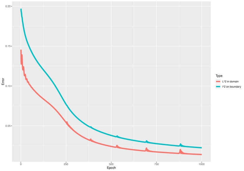
Figure 6: Training loss (i.e. $\ell^{2}(\Gamma)$-error) and $L^{2}(\Omega)$-error over 1 000 Adam epochs for a sample manufactured solution.

4.2 Dependence on the order of one multipole expansion

Instead of multiple multipole expansions, let us now train one expansion (one center) of a given order (which we vary). As initial position for the center we choose a random point outside $\Omega$ and inside the square centered in the origin with side length 4, while the initial coefficients of the expansion are obtained from the collocation method for this center.

The Adam algorithm is then run for a number of epochs until the training loss becomes smaller than 0.05, for at most $5\cdot 10^{5}$ epochs. The learning rate is 0.1 and the batch size is the full dataset.

We perform this procedure for 100 manufactured solutions, each centered on an equidistant point of the curve 10 with parameters $\alpha=0.8$, $\beta=1$, $\gamma=0.2$, and $N=5$ (see Figure 4b).

Figure 7 shows the normalized $L^{2}(\Omega)$-error produced by the initial position and after the Adam optimization. The order of the multipole expansion is in the range $[1,3]$.

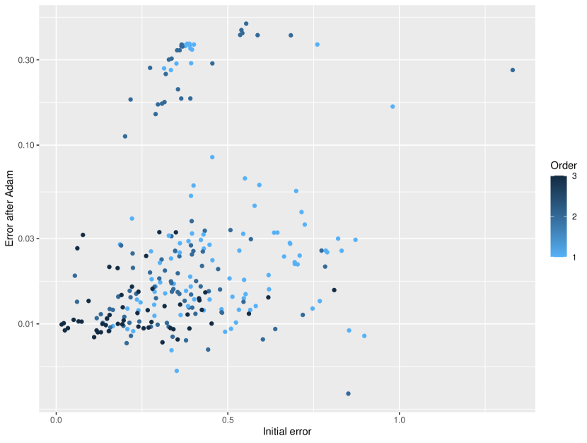
Figure 7: $L^{2}(\Omega)$-error before and after the Adam optimization (one multipole expansion with different orders).

Similarly to Figure 5, while the initial error shows considerable variation, the final relative error tends to stabilize at a median value of $\approx$ 1.62%. Contrarily to Figure 5, for no observation the final error is larger than the initial one.

Moreover, a single multipole expansion could also be used to find the center of the singularity of 1 itself. In fact, the best position for the multipole expansion to approximate 1 should be at the singularity itself. This could be proven by contradiction by taking a circle with radius $\rho$ and considering the $\ell^{2}(\Gamma)$-error for a multipole expansion centered at a point of this circle. This error will depend on $\rho$ and become minimal when $\rho=0$.

Figure 8 shows the $\ell^{2}$-distance between the singularity of the solution and the center of one multipole expansion before and after the Adam optimization. In 12.16% of observations the initial distance is smaller than the one after the Adam optimization: however, in all these cases the training loss did not become smaller than 0.05 in $5\cdot 10^{5}$ epochs.

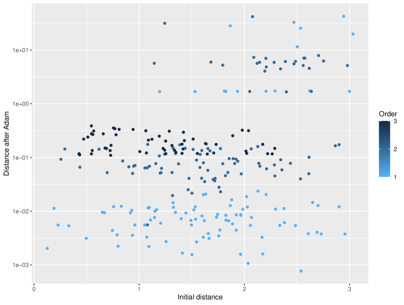
Figure 8: $\ell^{2}$-distance between solution and expansion before and after the Adam optimization (one multipole expansion with different orders).

4.3 Implementation

Our code is written in Python 3.

For meshing and numerical integration, we rely on Netgen/NGSolve (TU Wien, 2019). For the Adam optimization, we rely on PyTorch (Facebook AI Research, 2020). By defining a new torch.nn.Module for the first and second layer of the MMP ansatz as a neural network (Section 3), we can use the automatic differentiation tool of PyTorch for the Jacobians needed by the backpropagation step of the Adam algorithm. Furthermore, we exploit the PyTorch parallelization on GPUs when training each neural network and the Python multiprocessing module to parallelize over the manufactured solutions.

5 Conclusions

We have shown that gradient-based optimization algorithms commonly used to train neural networks, such as the Adam algorithm, can help with overcoming a flaw of MAS, namely the heuristics needed to place its point sources, by optimizing with respect to these positions (together with the coefficients of the point sources).

Future work will involve 1) applying this approach to other problems, i.e. with different boundaries, manufactured solutions, and PDEs, and 2) using a genetic algorithm to optimize also with respect to the number and orders of the multipole expansions (total number of degrees of freedom of MMP). These are the metaparameters of the MMP ansatz as a neural network, which now have to be chosen by the user. A too large number of degrees of freedom for MMP should be penalized by the genetic procedure.

References

- Abramowitz & Stegun (1964) Abramowitz, M. and Stegun, I. A. Handbook of Mathematical Functions with Formulas, Graphs, and Mathematical Tables. Dover, New York, NY, 9th edition, 1964.
- Alparslan & Hafner (2016) Alparslan, A. and Hafner, C. Current status of MMP analysis of photonic structures in layered media. In 2016 IEEE/ACES International Conference on Wireless Information Technology and Systems (ICWITS) and Applied Computational Electromagnetics (ACES), pp. 1–2, 2016. doi: 10.1109/ROPACES.2016.7465317.
- Brenner & Scott (2008) Brenner, S. C. and Scott, L. R. The Mathematical Theory of Finite Element Methods, volume 15 of Texts in Applied Mathematics. Springer, New York, NY, 3rd edition, 2008. doi: 10.1007/978-0-387-75934-0.
- Carrascal et al. (1991) Carrascal, B., Estevez, G., Lee, P., and Lorenzo, V. Vector spherical harmonics and their application to classical electrodynamics. European Journal of Physics, 12(4):184–191, 1991. doi: 10.1088/0143-0807/12/4/007.
- Casati & Hiptmair (2019) Casati, D. and Hiptmair, R. Coupling finite elements and auxiliary sources. Computers & Mathematics with Applications, 77(6):1513–1526, 2019.
- Facebook AI Research (2020) Facebook AI Research. PyTorch v17.0, 2020. URL https://pytorch.org.
- Gamelin (2001) Gamelin, T. W. Complex Analysis. Undergraduate Texts in Mathematics. Springer, New York, NY, 1st edition, 2001. doi: 10.1007/978-0-387-21607-2.
- Griffiths (2013) Griffiths, D. J. Introduction to Electrodynamics. Pearson, Boston, MA, 4th edition, 2013. Republished by Cambridge University Press in 2017.
- Hafner (1980) Hafner, C. Beiträge zur Berechnung der Ausbreitung elektromagnetischer Wellen in zylindrischen Strukturen mit Hilfe des “Point-Matching”-Verfahrens. PhD thesis, ETH Zurich, Switzerland, 1980. URL https://doi.org/10.3929/ethz-a-000220926.
- Hafner (1999) Hafner, C. Chapter 3 - The Multiple Multipole Program (MMP) and the Generalized Multipole Technique (GMT). In Wriedt, T. (ed.), Generalized Multipole Techniques for Electromagnetic and Light Scattering, pp. 21–38. Elsevier, Amsterdam, 1999. doi: 10.1016/B978-044450282-7/50015-4.
- Haykin (2008) Haykin, S. Neural Networks and Learning Machines. Pearson, 3rd edition, 2008.
- Heretakis et al. (2005) Heretakis, I. I., Papakanellos, P. J., and Capsalis, C. N. A stochastically optimized adaptive procedure for the location of mas auxiliary monopoles: the case of electromagnetic scattering by dielectric cylinders. IEEE Transactions on Antennas and Propagation, 53(3):938–947, 2005. doi: 10.1109/TAP.2004.842699.
- Hiptmair (2002) Hiptmair, R. Finite elements in computational electromagnetism. Acta Numerica, 11, 2002. doi: 10.1017/S0962492902000041.
- Hiptmair et al. (2016) Hiptmair, R., Moiola, A., and Perugia, I. A survey of Trefftz methods for the Helmholtz equation. In Barrenechea, G. R., Brezzi, F., Cangiani, A., and Georgoulis, E. H. (eds.), Building Bridges: Connections and Challenges in Modern Approaches to Numerical Partial Differential Equations, pp. 237–279. Springer, Cham, 2016. doi: 10.1007/978-3-319-41640-3˙8.
- Kingma & Ba (2015) Kingma, D. P. and Ba, J. Adam: A method for stochastic optimization. In Bengio, Y. and LeCun, Y. (eds.), 3rd International Conference on Learning Representations, ICLR 2015, San Diego, CA, USA, May 7–9, 2015, Conference Track Proceedings, 2015. URL http://arxiv.org/abs/1412.6980.
- Koch et al. (2018) Koch, U., Niegemann, J., Hafner, C., and Leuthold, J. MMP simulation of plasmonic particles on substrate under e-beam illumination. In Wriedt, T. and Eremin, Y. (eds.), The Generalized Multipole Technique for Light Scattering: Recent Developments, pp. 121–145. Springer, Cham, 2018. doi: 10.1007/978-3-319-74890-0˙6.
- Kupradze & Aleksidze (1964) Kupradze, V. D. and Aleksidze, M. A. The method of functional equations for the approximate solution of certain boundary value problems. USSR Computational Mathematics and Mathematical Physics, 4(4):82–126, 1964. doi: 10.1016/0041-5553(64)90006-0.
- Mie (1900) Mie, G. Elektrische Wellen an zwei parallelen Drähten. Annalen der Physik, 307:201–249, 1900. doi: 10.1002/andp.19003070602.
- Moiola (2011) Moiola, A. Trefftz-Discontinuous Galerkin Methods for Time-Harmonic Wave Problems. PhD thesis, Seminar for Applied Mathematics, ETH Zurich, Switzerland, 2011. URL https://www.doi.org/10.3929/ethz-a-006698757.
- (20) Moreno, E., Erni, D., Hafner, C., and Vahldieck, R. Multiple multipole method with automatic multipole setting applied to the simulation of surface plasmons in metallic nanostructures. Journal of the Optical Society of America A, 19(1):101–111. doi: 10.1364/JOSAA.19.000101.
- Rall (1981) Rall, L. B. Automatic differentiation: Techniques and applications, volume 120 of Lecture Notes in Computer Science. Springer, 1st edition, 1981. doi: 10.1007/3-540-10861-0.
- Ramachandran et al. (2017) Ramachandran, P., Zoph, B., and Le, Q. V. Searching for activation functions. Computing Research Repository, 2017. URL http://arxiv.org/abs/1710.05941.
- Sakakibara (2016) Sakakibara, K. Analysis of the dipole simulation method for two-dimensional Dirichlet problems in Jordan regions with analytic boundaries. BIT Numerical Mathematics, 56(4):1369–1400, 2016. doi: 10.1007/s10543-016-0605-1.
- TU Wien (2019) TU Wien. Netgen/NGSolve v6.2, 2019. URL https://ngsolve.org.
- Vekua (1967) Vekua, I. N. New Methods for Solving Elliptic Equations. North Holland Publishing Company, 1st edition, 1967.
- Yee (1966) Yee, K. Numerical solution of initial boundary value problems involving Maxwell’s equations in isotropic media. IEEE Transactions on Antennas and Propagation, 14(3):302–307, 1966. doi: 10.1109/TAP.1966.1138693.
- Zaridze et al. (2000) Zaridze, R. S., Bit-Babik, G., Tavzarashvili, K., Uzunoglu, N. K., and Economou, D. P. The Method of Auxiliary Sources (MAS) — Solution of propagation, diffraction and inverse problems using MAS. In Uzunoglu, N. K., Nikita, K. S., and Kaklamani, D. I. (eds.), Applied Computational Electromagnetics: State of the Art and Future Trends, volume 171 of NATO ASI Series, pp. 33–45. Springer, Berlin, Heidelberg, 2000. doi: 10.1007/978-3-642-59629-2˙3.