Semi-Synchronous Federated Learning for Energy-Efficient Training and Accelerated Convergence in Cross-Silo Settings
Abstract.
There are situations where data relevant to machine learning problems are distributed across multiple locations that cannot share the data due to regulatory, competitiveness, or privacy reasons. Machine learning approaches that require data to be copied to a single location are hampered by the challenges of data sharing. Federated Learning (FL) is a promising approach to learn a joint model over all the available data across silos. In many cases, the sites participating in a federation have different data distributions and computational capabilities. In these heterogeneous environments existing approaches exhibit poor performance: synchronous FL protocols are communication efficient, but have slow learning convergence and high energy cost; conversely, asynchronous FL protocols have faster convergence with lower energy cost, but higher communication. In this work, we introduce a novel energy-efficient Semi-Synchronous Federated Learning protocol that mixes local models periodically with minimal idle time and fast convergence. We show through extensive experiments over established benchmark datasets in the computer-vision domain as well as in real-world biomedical settings that our approach significantly outperforms previous work in data and computationally heterogeneous environments.
1. Introduction
Data useful for a machine learning problem is often generated at multiple, distributed locations. In many situations these data cannot be exported from their original location due to regulatory, competitiveness, or privacy reasons. A primary motivating example is health records, which are heavily regulated and protected, restricting the ability to analyze large datasets. Industrial data (e.g., accident or safety data) is also not shared due to competitiveness reasons. Additionally, given recent high-profile data leak incidents more strict data ownership laws have been enacted, such as the European Union’s General Data Protection Regulation (GDPR), China’s Cyber Security Law and General Principles of Civil Law, and the California Consumer Privacy Act (CCPA).
These situations bring data distribution, security, and privacy to the forefront of machine learning and impose new challenges on how data should be shared and analyzed. Federated Learning (FL) is a promising solution (McMahan et al., 2017a; Konečnỳ et al., 2016; Yang et al., 2019), which can help learn deep neural networks from data silos (Jain, 2003) by collaboratively training models that aggregate locally-computed updates (e.g., gradients) under a centralized (e.g., central parameter server) or a decentralized (e.g., peer-to-peer) learning topology (Li et al., 2020d; Bellavista et al., 2021), while providing strong privacy and security guarantees (e.g., (Bonawitz et al., 2017; Zhang et al., 2020)). Models trained using Federated Learning outperform the models that any individual participant in the federation could achieve by training solely on its local data (cf. Figure 12).
Our primary interest is to develop efficient Federated Learning training policies for the data center setting (Li et al., 2020d) that accelerate learning convergence while minimizing computational, communication, and energy costs. In particular, we target cross-silo Federated Learning environments (Kairouz and McMahan, 2021; Yang et al., 2019; Li et al., 2020d; Rieke et al., 2020; Zhang et al., 2020), such as a network of hospitals or a research consortium that wants to jointly learn a model without sharing any data. In these environments, participants often have different computational capabilities (system heterogeneity) and different local data distributions (statistical heterogeneity). Current Federated Learning approaches use either synchronous (McMahan et al., 2017a; Smith et al., 2017; Bonawitz et al., 2019) or asynchronous (Xie et al., 2020) communication protocols. However, these methods have poor performance in such heterogeneous environments. Synchronous protocols result in computationally fast learners being idle, underutilizing the available resources of the federation. Asynchronous protocols fully utilize the available resources, but incur higher network communication cost and potentially lower generalizability due to the effect of stale models (Cui et al., 2014; Dai et al., 2019).
To address these challenges, we introduce a new hybrid training scheme, Semi-Synchronous Federated Learning (SemiSync), which allows learners to continuously train on their local dataset up to a specific temporally specified synchronization point where the current local models of all learners are aggregated to compute the community model. This approach produces better utilization of the federation resources, while limiting communication costs. We empirically demonstrate the effectiveness of this new scheme in terms of convergence time, communication cost and energy efficiency on a variety of challenging learning environments with diverse computational resources, variable data amounts, and different target class distributions (IID and Non-IID example assignments) across learners. Our training scheme leads to faster convergence regardless of the optimizer used to train the local models. Our contributions are:
-
•
A new Semi-Synchronous communication protocol for cross-silo Federated Learning settings with accelerated convergence, and reduced communication, processing and energy cost.
-
•
A caching approach that enables computation of the community model in constant time in asynchronous Federated Learning environments.
-
•
A new asynchronous communication policy based on staleness, FedRec, which outperforms existing asynchronous learning policies.
-
•
A systematic evaluation of Federated Learning training policies on standard benchmarks and on a challenging neuroimaging dataset over diverse federated learning environments.
2. Related Work
Federated Learning was introduced by McMahan et al. ((2017a)) for user data in mobile phones. Their original algorithm, Federated Average, follows a synchronous communication protocol where each learner (phone) trains a neural network for a fixed number of epochs on its local dataset. Once all learners (or a subset) finish their locally assigned training, the system (i.e., federation controller) computes a community model that is a weighted average of each of the learners’ local models, with the weight of each learner in the federation being equal to the number of its local training examples. The new community model is then distributed to all learners and the process repeats. This approach, which we call SyncFedAvg, has catalyzed much of the recent work (Smith et al., 2017; Bonawitz et al., 2019; Li et al., 2020d).
SGD Optimization.
The FL settings that we investigate in this work are related to stochastic optimization in distributed and parallel systems (Bertsekas, 1983; Bertsekas and Tsitsiklis, 1989), as well as in synchronous distributed stochastic gradient descent (SGD) optimization (Chen et al., 2016). The problem of delayed (i.e., stale) gradient updates due to asynchronicity is well known (Lian et al., 2015; Recht et al., 2011; Agarwal and Duchi, 2011), with (Lian et al., 2015) providing theoretical support for nonconvex optimization functions under the IID assumption. In our work, we study FL in more general, Non-IID settings.
Periodic SGD
Our SemiSync policy is related to parallel training policies such as Elastic and Periodic SGD Averaging (Zhang et al., 2015; Wang and Joshi, 2018; Reisizadeh et al., 2020), where a central server aggregates the learners local gradient updates when a specific number of iterations is complete. This periodic aggregation controls the communication frequency between every learner and the server. Zhang et al. (Zhang et al., 2015) introduce an elastic update rule around an average global variable consensus for IID settings. Wang and Joshi (Wang and Joshi, 2018) provide a general analysis framework for different cooperative learning environments. FedPAQ (Reisizadeh et al., 2020) studies the convergence guarantees of periodic averaging in cross-device IID settings for strongly convex and non-convex functions with quantized message-passing. In contrast, we study time-based periodic averaging when the participating learners have highly diverse computational resources and data distributions. We define the synchronization time period based on the data amounts and computational power of the learners, as multiples/fractions of the time it takes for the slowest learner in the federation to complete a single epoch, instead of epoch-level (McMahan et al., 2017a) or iteration-level (Reisizadeh et al., 2020) synchronization, or performance tiers (Chai et al., 2020).
Global and Local Model Optimization.
In statistically heterogeneous FL settings clients can drift too far away from the global optimal model. An approach to tackle client drift is to decouple the SGD optimization into local (learner side) and global (server side) (Reddi et al., 2020; Hsu et al., 2019). Hsu et al. (Hsu et al., 2019) investigate a server-side momentum-based update rule (FedAvgM) between the previous community model and the newly computed weighted average of the clients’ models. Reddi et al. (Reddi et al., 2020) introduce a more generalized server-side optimization update rule (FedOpt) with support for adaptive SGD optimizers (FedAdagrad, FedYogi, FedAdam). FedProx (Li et al., 2020d) directly addresses client drift by introducing a regularization term in the clients local objective, which penalizes the divergence of the local solution from the global solution. FedAsync (Xie et al., 2020) weights the different local models based on their staleness with respect to the latest community model. Liu et al (Liu et al., 2020) show that using Momentum SGD as the local model solver leads to accelerated convergence compared to Vanilla SGD. In our setting, we study the effect of local models mixing strategies under different communication protocols, as well as the effect of local model solvers (i.e., Vanilla SGD, Momentum SGD and FedProx) on the convergence rate of the global model.
Federated Convergence Guarantees.
FedProx studied the convergence rate of FedAvg over dissimilar learners’ local solutions (Li et al., 2020d). Wang et al. (Wang et al., 2019) studied adaptive FL in mobile edge computing environments under resource budget constraints with arbitrary local updates between learners. Li et al. (Li et al., 2020b) provide convergence guarantees over full and partial device participation for FedAvg. Chen et al. (Chen et al., 2020) formulated a joint federated learning optimization problem targeting optimal resource allocation and client selection in wireless networks. FedAsync (Xie et al., 2020) provides convergence guarantees for asynchronous environments and a community model that is a weighted average of local models based on staleness. In our work, we empirically study the convergence of the different federated learning protocols on computationally heterogeneous environments on IID and Non-IID data distributions with full client participation in the cross-silo (data center) FL settings with the presence of stragglers (Dean and Barroso, 2013), instead of partial client participation (Li et al., 2020d; McMahan et al., 2017a), dropouts (Chai et al., 2020).
Federated Learning Energy Efficiency
Most of the recent work on energy consumption in FL settings focuses on the energy cost of decentralized training on wireless networks (Luo et al., 2020; Yang et al., 2020; Tran et al., 2019). Luo et al. (Luo et al., 2020) consider the problem of cost-effective FL design which jointly optimizes learning time and energy consumption on the edge with convergence guarantees. The works of (Tran et al., 2019; Yang et al., 2020) study the trade-off of computation and communication latency in decentralized FL and its effect on total energy consumption, system learning time and learning accuracy. In our work, however, we analyze the energy efficiency of federated learning training protocols in cross-silo (data center) settings. As it is also shown in (Shehabi et al., 2016) energy consumption in data centers is of notable importance due to its considerable environmental impact, while the work of (Masanet et al., 2020) stresses the need for additional energy consumption analysis tools that can monitor more accurately energy efficiency and help advance sustainability in data center settings.
Federated Learning in Healthcare.
Federated Learning holds great promise for the future of digital health and cross-institutional healthcare informatics (Rieke et al., 2020). FL has been used for phenotype discovery (Liu et al., 2019), for patient representation learning (Kim et al., 2017), and for identifying similar patients across institutions (Lee et al., 2018). FL has been applied to a variety of tasks in biomedical imaging, including whole-brain segmentation of MRI T1 scans (Roy et al., 2019), brain tumor segmentation (Sheller et al., 2018; Li et al., 2019), multi-site fMRI classification and identification of disease biomarkers (Li et al., 2020a), and for identification of brain structural relationships across diseases and clinical cohorts using (federated) dimensionality reduction from shape features (Silva et al., 2019). Silva et al. (Silva et al., 2020) present an open-source FL framework for healthcare that can support different machine learning models and optimization methods. COINSTAC (Plis et al., 2016) provides a distributed privacy-preserving computation framework for neuroimaging. We apply FL to brain age estimation from structural MRI scans that are distributed across different data silos (cf. Section 6).
Privacy.
Our proposed Semi-Synchronous training protocol can be run under standard privacy techniques such as differential privacy (Abadi et al., 2016b; McMahan et al., 2017b), secure multi-party computation (MPC) (Bonawitz et al., 2017; Mohassel and Zhang, 2017; Kilbertus et al., 2018), and homomorphic encryption (Rivest et al., 1978; Paillier, 1999a; Zhang et al., 2020; Stripelis et al., 2021b). Currently, we are actively working on a Paillier based additive homomorphic encryption scheme (Paillier, 1999b) that will encompass all the different training protocols we discuss in this work. We refer the reader to our current progress for additional details (Stripelis et al., 2021b). Further analysis of privacy techniques is out of scope, since our goal is to evaluate the performance of federated learning training policies in heterogeneous cross-silo settings (Stripelis et al., 2021b).
3. Federated Optimization
In Federated Learning the goal is to find the optimal set of parameters that minimize the global objective function:
| (1) |
where N denotes the number of participating learners, the contribution of learner in the federation, the normalization factor (), and the local objective function of learner . We refer to the model computed using Equation 1 as the community model . Every learner computes its local objective by minimizing the empirical risk over its local training set as , with being the loss function. For example, in the FedAvg weighting scheme, the contribution value for any learner is equal to its local training set size, . The contribution value can be static, or dynamically defined at run time (cf. Section 4).
In the original Federated Learning work (McMahan et al., 2017a) every learner aims to minimize its local function using Vanilla Stochastic Gradient Descent (SGD) as its local solver ( learning rate):
| (2) |
In SGD with Momentum (which can accelerate convergence (Liu et al., 2020)), the local solution at iteration is computed as ( momentum term, momentum attenuation factor):
| (3) |
FedProx (Li et al., 2020d) is a variant of the local SGD solver that introduces a proximal term in the update rule to regularize the local updates based on the divergence of the local solution from the global solution (i.e., the community model ). The local solution is computed as:
| (4) |
The proximal term controls the divergence of the local solution from the global. In this work, we study the effectiveness of the Semi-Synchronous protocol for all three local SGD solver variants.
4. Federated Learning Policies
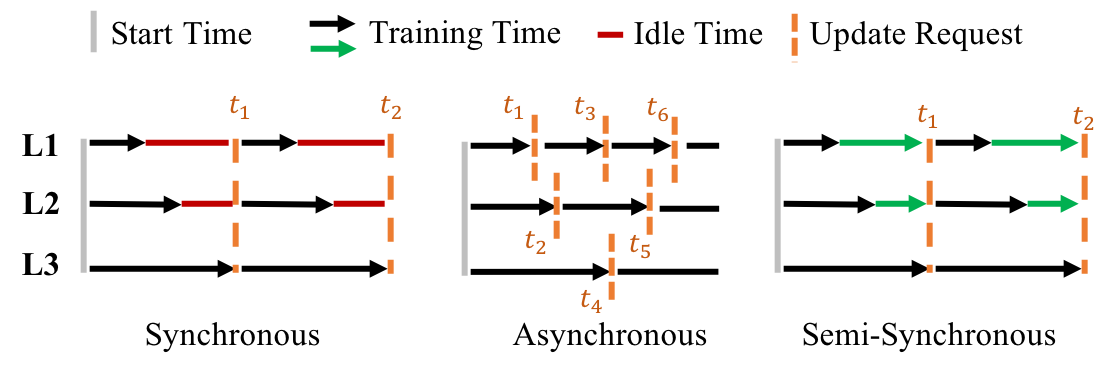
In this section we review the main characteristics of synchronous and asynchronous federated learning policies, and introduce our novel semi-synchronous policy. Figure 1 sketches their training execution flow. We compare these approaches under three evaluation criteria: convergence time, communication cost and energy cost. Rate of convergence is expressed in terms of parallel processing time, that is, the time it takes the federation to compute a community model of a given accuracy with all the learners running in parallel. Communication cost is measured in terms of update requests, that is, the number of local models sent from any learner to the controller during training. Each learner also receives a community model after each request, so the total number of models exchanged is twice the update requests. Energy cost is based on the cumulative processing time (total wall-clock time across learners required to compute the community model) and on the energy efficiency of each learner (e.g., GPU, CPU). Table 1 summarizes our findings (cf. Section 6).
| Protocol | processing cost | communication cost | energy cost | idle-free | stale-free |
|---|---|---|---|---|---|
| synchronous | high | low | high | x | ✓ |
| asynchronous | low | high | medium | ✓ | x |
| semi-synchronous | low | low | low | ✓ | ✓ |
4.1. Synchronous Federated Learning
Under a synchronous communication protocol, each learner performs a given number of local steps (usually expressed in terms of local epochs). After all learners have finished their local training, they share their local models with the centralized server (federation controller) and receive a new community model. This training procedure continues for a number of federation rounds (synchronization points). This is a well-established training approach with strong theoretical guarantees and robust convergence for both IID and Non-IID data (Li et al., 2020b; McMahan et al., 2017a).
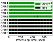
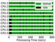
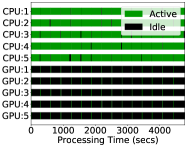
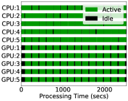
However, a limitation of synchronous policies is their slow convergence due to waiting for slow learners (stragglers (Dean and Barroso, 2013)). For a federation of learners with heterogeneous computational capabilities, fast learners remain idle most of the time, since they need to wait for the slow learners to complete their local training before a new community model can be computed (Figure 1). As we move towards larger networks, this resource underutilization is exacerbated. Figure 2(a,b) shows idle times of a synchronous protocol when training a 2-CNN (a) or a ResNet-50 (b) network in a federation with fast (GPU) and slow (CPU) learners. The fast learners are severely underutilized.
4.2. Asynchronous Federated Learning
In asynchronous Federated Learning no synchronization point exists and learners can request a community update from the controller whenever they complete their local assigned training. Asynchronous protocols have faster convergence speed since no idle time occurs for any of the participating learners. However, they incur higher communication cost and lower generalizability due to staleness (Cui et al., 2014; Dai et al., 2019). Figure 1(center) illustrates a typical asynchronous policy. The timestamps represent the update requests issued by the learners to the federation controller. No synchronization exists and every learner issues an update request at its own learning pace. All learners run continuously, so there is no idle time.
Since in asynchronous protocols, no strict consistency model (Lamport, 1979) exists, it is inevitable for learners to train on stale models. Community model updates are not directly visible to all learners and different staleness degrees may be observed (Ho et al., 2013; Cui et al., 2014). Recently, FedAsync (Xie et al., 2020) was proposed as an asynchronous training policy for Federated Learning by weighting every learner in the federation based on functions of model staleness. FedAsync defines staleness as the difference between the current global timestamp (vector clock (Mattern et al., 1988)) of the community model and the global timestamp associated with the committing model of a requesting learner. Specifically, for learner , its staleness value is equal to , (i.e., FedAsync Poly) with being the current global clock value and the global clock value of the committing model of the requesting learner.
Given that staleness can also be controlled by tracking the total number of iterations or number of steps (i.e., batches) applied on the community model, we propose a new asynchronous protocol, FedRec, which weights models based on recency, extending the notion of effective staleness in (Dai et al., 2019; Dai, 2018). For each model we define the number of steps that were performed in its computation. Assume a learner that receives a community model at time , which was computed over a cumulative number of steps (the sum of steps used by each of the local models involved in computing the community model). Learner then performs local steps starting from this community model, and requests a community update at time . By that time the current community model may contain steps, since other learners may have contributed steps between and . Therefore, the effective staleness weighting value of learner in terms of steps is (following the FedAsync + Poly function). When , is set to 1. As shown in Section 6, the step-based recency/staleness function of FedRec outperforms the time-based staleness function of FedAsync (cf. Figures 8, 9, 10).
4.3. Semi-Synchronous Federated Learning
We have developed a novel Semi-Synchronous training policy that seeks to balance resource utilization and communication costs111In our cross-silo settings, we do not consider delays due to learners’ transmission speed. In our experiments in Section 6 model transmission time is less than 0.5% of the computation time. (cf. Figure 2). In this policy every learner continues training up to a specific synchronization time point (cf. Figure 1(right)). The synchronization point is based on the maximum time it takes for any learner to perform a single epoch (). Specifically:
| (5) |
where refers to the local training data size of learner , to the batch size of learner and to the time it takes learner to perform a single step (i.e., process a single batch). The hyperparameter controls the number of local passes the slowest learner in the federation needs to perform before all learners synchronize. For example, refer to the slowest learner completing two epochs. The hyperparmeter can be fractional, that is, the slowest learner may only process part of its training set in a federation round. The term denotes the number of steps (batches) learner needs to perform before issuing an update request, which depends on its computational speed. A theoretical analysis of the weight divergence of our proposed Semi-Synchronous training scheme compared to the centralized model and a more detailed formulation of the federated optimization problem can be found in the Appendix.
To compute the necessary statistics (i.e. time-per-batch per learner), SemiSync performs an initial cold start federation round (see GPUs in Figure 2(b,d)) where every learner trains for a single epoch and the controller collects the statistics to synchronize the new SemiSync federation round. Here, the hyperparameter and the timings per batch are kept static throughout the federation training once defined, although others schedules are possible (cf. Section 7). To obtain a good estimate of the processing time per batch, in the cold start phase the system has every learner complete a full epoch. The system sets a maximum duration for cold start to prevent a very slow learner from disrupting the federation.
In our SemiSync approach, the learners’ synchronization point does not depend on the number of completed epochs, but on the synchronization period. Learners with different computational power and amounts of data perform a different number of epochs, including fractional epochs. There is no idle time. Since the basic unit of computation is the batch, this allows for a more fine-grained control on when a learner contributes to the community model. This policy is particularly beneficial in heterogeneous computational and data distribution environments.
4.4. Training Policies Cost Analysis
Parallel Processing Time
We are interested in the wall-clock time it takes the federation to reach a community model of a given accuracy, with all learners running in parallel. For synchronous and semi-synchronous protocols, this is simply the number of federation rounds () times the synchronization period () (Luo et al., 2020). For asynchronous protocols, this is the time at which a learner submits the last local model that makes the community model reach the desired accuracy (e.g., time in Figure 1). If denotes the processing time difference between update requests, and the number of update requests, then the total parallel processing time is computed as:
| (6) |
Communication Cost
We measure communication cost by the total number of update requests issued during training by the learners to the federation controller. Each update request accounts for two model exchanges: the learner sends its local model to the controller and receives the community model. In a federation of learners, for synchronous and semi-synchronous protocols with synchronization points, and for asynchronous with update requests:
| (7) |
Energy Cost
The energy cost is based on the cumulative processing time of all learners to complete their local training (Luo et al., 2020) weighted by the energy cost () of each learner’s processor (e.g., GPU or CPU). For asynchronous protocols, let denote the total number of local epochs performed by a learner k to reach a particular timestamp, then the cumulative energy cost is:
| (8) |
5. Federated Learning Environment
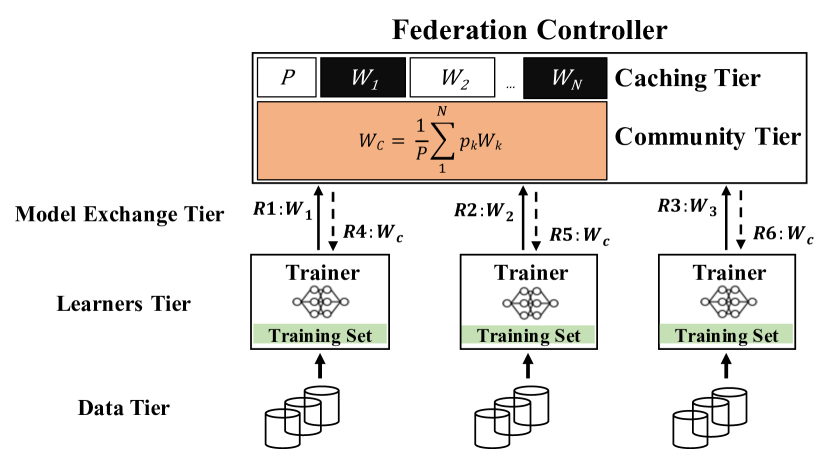
We have designed and developed a flexible Federated Learning system, called Metis, to explore different communication protocols and model aggregation weighting schemes (Figure 3). Metis uses Tensorflow (Abadi et al., 2016a) as its deep learning execution engine. In Figure 3, we decompose the federated learning environment into tiers in order to exemplify the data management and training procedures occurring in cross-silo settings.
Federation Controller
The centralized controller is a multi-threaded process with a modular design that integrates a collection of extensible microservices (e.g., caching and community tiers). The controller orchestrates the execution of the entire federation and is responsible to initiate the system pipeline, broadcast the initial community model and handle learners’ update requests. Every incoming update request is handled by the controller in a FIFO ordering through a mutual exclusive lock, ensuring system state linearizability (Herlihy and Wing, 1990). Essentially, the federation controller is a materialized version of the Parameter Server (Abadi et al., 2016a; Dean et al., 2012) concept, widely used in distributed learning applications. The centralized (star-shaped (Bellavista et al., 2021)) federated learning topology that we investigate in this work, i.e., a centralized coordinator and a collection of learning nodes, is considered a standard topology in cross-silo federated learning settings (Li et al., 2020c; Yang et al., 2019; Kairouz and McMahan, 2021). Compared to existing work (Bonawitz et al., 2019; Wang et al., 2020; Gao et al., 2020) that follows a hierarchical structure, where multiple coordinators may exist along with a set of master/cloud-networks and sub-aggregators/fog-networks, our learning environment consists of a single master coordinator (i.e., Federation Controller) that is responsible for coordinating the federated execution and aggregating the learners’ local models.
Community & Caching Tier.
The community tier computes a new community model as a weighted average of the most recent model that each learner has shared with the controller (Eq. 1). To facilitate this computation, it is natural to store the most recently received local model of every learner in-memory or on disk. Therefore, the memory and storage requirements of a community model depend on the number of learners contributing to the community model. Similarly to the computation of the community model in synchronous protocols, we extend this approach to asynchronous protocols by using our proposed caching scheme at every update request. For synchronous protocols we always need to perform a pass over the entire collection of stored local models, with a computational cost , where is the size of the model and is the number of participating learners. For asynchronous protocols where learners generate update requests at different paces and the total number of update requests is far greater than synchronous, such a repetitive complete pass is expensive and we can leverage the existing cached/stored local models to compute a new community model in time, independent of the number of learners.
Consider an unnormalized community model consisting of matrices, , and a community normalization weighting factor . Given a new request from learner , with new community contribution value , the new normalization value is , where is the learner’s previous contribution value. For every component matrix of the community model, the updated matrix is , where are the new and existing component matrices of learner . The new community model is . Using this caching approach, in asynchronous execution environments, the most recently contributed local model of every learner in the federation is always considered in the community model.
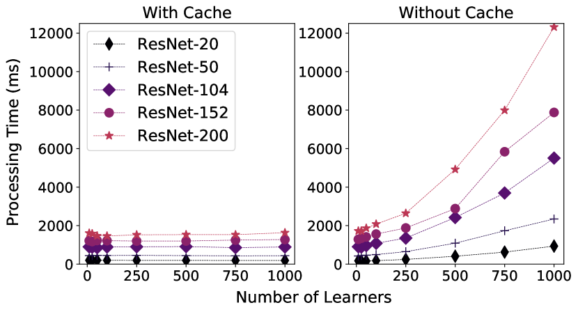
Some existing asynchronous community mixing approaches (Xie et al., 2020; Sprague et al., 2018) compute a weighted average using a mixing hyperparameter between the current community and the committing local model of a requesting learner. In contrast, our caching approach eliminates this mixing hyperparameter dependence and performs a weighted aggregation using all recently contributed local models. Figure 4 shows the computation cost for different sizes of a ResNet community model (from Resnet-20 to Resnet-200), in the CIFAR-100 domain, as the federation increases to 1000 learners. With our caching mechanism the time to compute a community model remains constant irrespective of the number of participating learners, while it significantly increases without it.
Model Exchange Tier.
This tier follows a stateful client-server communication architecture (Hauswirth and Jazayeri, 1999). Every learner in the federation contacts the controller for a community update once it completes its locally assigned training and shares its local model with the controller. Upon computing the new community model, in the synchronous and semi-synchronous cases, the controller broadcasts the new model to all learners, while in the asynchronous case, the controller sends the new model to the requesting learner. Figure 3 represents the model exchange of the semi/synchronous cases with requests R1 to R6.
Learners & Data Tier.
In the current work, all learners train on the same neural network architecture with identical hyperparameter values (learning rate, batch size, etc.), starting from the same initial (random) model state, and using the same local SGD optimizer (but see future work in Section 7). The number of local steps a learner performs before issuing an update request are defined either in terms of epochs/batches or the maximum scheduled time (see Eq. 5). Every learner trains on its own local training dataset and no data is shared.
Execution Pipeline.
Algorithm 1 describes the execution pipeline within Metis for synchronous, semi-synchronous and asynchronous communication protocols. In synchronous and semi-synchronous protocols, the controller waits for all the participating learners to finish their local training task before it computes a community model, distribute it to the learners, and proceed to the next global iteration. In asynchronous protocols, the controller computes a community model whenever a single learner finishes its local training, using the caching mechanism, and sends the new model to the learner. In all cases, the controller assigns a contribution value to the local model that a learner shares with the community. For synchronous and asynchronous FedAvg (SyncFedAvg and AsyncFedAvg), this value is statically defined and based on the size of the learner’s local training dataset, . For other weighting schemes, such as FedRec, the Staleness procedure computes it dynamically. The LearnerOpt procedure implements the local training of each learner. The local training task assignment information is passed to every learner through the metadata, , collection. Finally, a learner trains on its local model using either Vanilla SGD, Momentum SGD or FedProx as its local SGD solver.
6. Experiments
We conduct an extensive experimental evaluation of different training policies on a diverse set of federated learning environments with heterogeneous amounts of data per learner, local data distributions, and computational resources. We evaluate the protocols on the CIFAR-10, CIFAR-100 and ExtendedMNIST By Class (Cohen et al., 2017; Caldas et al., 2018) benchmark datasets with a federation consisting of 10 learners as well as on the BrainAge prediction task (Cole et al., 2017; Jónsson et al., 2019; Peng et al., 2020; Stripelis et al., 2021a; Gupta et al., 2021) with a federation of 8 learners. The asynchronous protocols (i.e., FedRec and AsyncFedAvg) were run using the caching mechanism described in Section 5 except for FedAsync. FedAsync was run using the polynomial staleness function, i.e., FedAsyncPoly, with mixing hyperparameter and model divergence regularization factor , which is reported to have the best performance (Xie et al., 2020).
Models Architecture.
The architecture of the deep learning networks for CIFAR-10 and CIFAR-100 come from the Tensorflow tutorials: for CIFAR-10 we train a 2-CNN222CIFAR-10: https://github.com/tensorflow/models/tree/r1.13.0/tutorials/image/cifar10 and for CIFAR-100 a ResNet-50333CIFAR-100: https://github.com/tensorflow/models/tree/r1.13.0/official/resnet. The 2-CNN model444ExtendedMNIST: https://github.com/TalwalkarLab/leaf/blob/master/models/femnist/cnn.py architecture for ExtendedMNIST comes from the LEAF benchmark (Caldas et al., 2018). The 5-CNN for BrainAge is from (Stripelis et al., 2021a). For all models, during training, we share all trainable weights (i.e., kernels and biases). For ResNet we also share the batch normalization, gamma and beta matrices. The random seed for all our experiments is set to 1990.
Models Hyperparameters.
For CIFAR-10 in homogeneous and heterogeneous environments the synchronous and semi-synchronous protocols were run with Vanilla SGD, Momentum SGD and FedProx; asynchronous protocols (FedRec, AsyncFedAvg) were run with Momentum SGD. For CIFAR-100 all the methods were run with Momentum (following the tutorial recommendation). For ExtendedMNIST By Class (following the benchmark recommendation) and BrainAge, we used Vanilla SGD. We originally performed a grid search, on the centralized model, over different combinations of learning rate , momentum factor , and mini batch size . For the proximal term in FedProx, we used the values from the original work (Li et al., 2020d). After identifying the optimal combination, we kept the hyperparameter values fixed throughout the federation training. In particular, for CIFAR-10 we used =0.05, =0.75, and =100, for CIFAR-100, =0.1, =0.9, =100, for ExtendedMNIST, =0.01 and =100, and for BrainAge = and =1. For both synchronous and asynchronous policies, we originally evaluated the convergence rate of the federation under different numbers of local epochs and we observed the best performance when assigning local epochs per learner. For the semi-synchronous case, we investigated the convergence of hyperparameter within the set .
Computational Environment.
Our homogeneous federation environment for CIFAR and ExtendedMNIST consists of 10 fast learners (GPUs) and our heterogeneous of 5 fast (GPU) and 5 slow (CPU) learners. For the BrainAge task our homogeneous environment consists of 8 fast learners. The fast learners were run on a dedicated GPU server equipped with 8 GeForce GTX 1080 Ti graphics cards of 10 GB RAM each, 40 Intel(R) Xeon(R) CPU E5-2630 v4 @ 2.20GHz, and 128GB DDR4 RAM. The slow learners were run on a separate server equipped with 48 Intel(R) Xeon(R) CPU E5-2650 v4 @ 2.20GHz and 128GB DDR4 RAM. For the 2-CNN used in CIFAR-10 the processing time per batch for fast learners is: , and for slow: , for the ResNet-50 used in CIFAR-100, for fast is: and for slow: , for the 2-CNN used in ExtendedMNIST for fast is: and for slow: and for the 5-CNN used in BrainAge for fast is: .
Data Distributions.
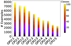
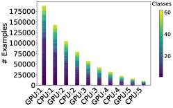
We evaluate the training policies over multiple environments with heterogeneous data sizes, data distributions, and learning problems (classification for CIFAR & ExtendedMNIST, regression for BrainAge).555CIFAR & ExtendedMNIST: https://dataverse.harvard.edu/dataset.xhtml?persistentId=doi%3A10.7910%2FDVN%2FPQ34F8 BrainAge: https://dataverse.harvard.edu/dataset.xhtml?persistentId=doi:10.7910/DVN/2RKAQP We consider three types of data size distributions: Uniform, where every learner has the same number of examples; Skewed, where each learner has a progressively smaller set of examples; and Power Law (exponent=1.5) to model extreme variations in the amount of data (intended to model the long tail of science). Learners train on all available local examples.
To model statistical heterogeneity in classification tasks, we assign a different number of examples per class per learner. Specifically, with IID we denote the case where all learners hold training examples from all the target classes, and with Non-IID(x) we denote the case where every learner holds training examples from only x classes. For example, Non-IID(3) in CIFAR-10 means that each learner only has training examples from 3 target classes (out of the 10 classes in CIFAR-10). For Power Law data sizes and Non-IID configurations, in order to preserve scale invariance, we needed to assign data from more classes to the learners at the head of the distribution. For example, for CIFAR-10 with Power Law and a goal of 5 classes per learner, the actual distribution is Non-IID(8x1,7x1,6x1,5x7), meaning that the first learner holds data from 8 classes, the second from 7 classes, the third from 6 classes, and all 7 subsequent learners hold data from 5 classes. For brevity, we refer to this distribution as Non-IID(5). Similarly for CIFAR-10 Power Law and Non-IID(3), the actual distribution is Non-IID(8x1,4x1,3x8). For CIFAR-100, Power Law and Non-IID(50), the actual distribution is Non-IID(84x1,76x1,68x1,64x1,55x1,50x5).
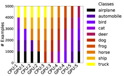
To model computational heterogeneity, we use fast (GPU) and slow (CPU) learners. In order to simulate realistic learning environments, we sort each configuration in descending data size order and assign the data to each learner in an alternating fashion (i.e., fast learner, slow learner, fast learner, etc.), except for the uniform distributions where the data size is identical for all learners. Due to space limitations, for every experiment we include the respective data distribution configuration as an inset in the convergence rate plots (Figures 7, 8, 9, 10, 11). Figure 5 shows three representative data distributions for the three classification domains.
The data distributions of the classification tasks that we investigate are based on the work of (Zhao et al., 2018), where the data are evenly (i.e, Uniform in our case) partitioned across 10 learners, and with different class distribution per learner (i.e., Non-IID(2) refers to examples from 2 classes per learner). We extend their work by also investigating the cases where the size of the partitions is not uniform, but follows a skewed or a power law distribution (called quantity skew/unbalanceness in (Kairouz and McMahan, 2021)).
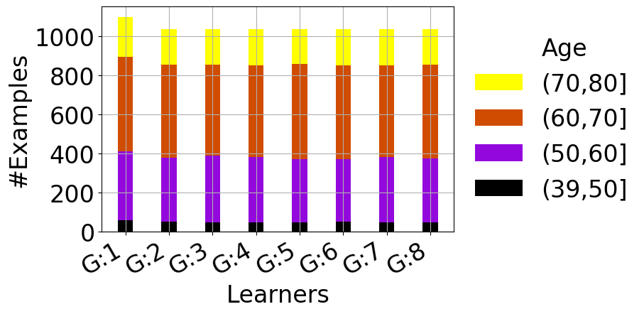
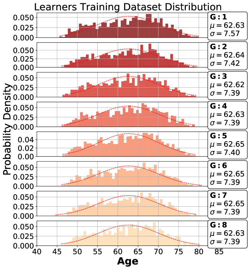
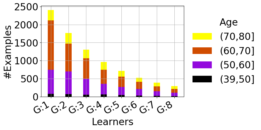
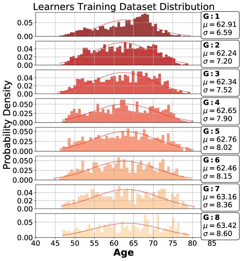
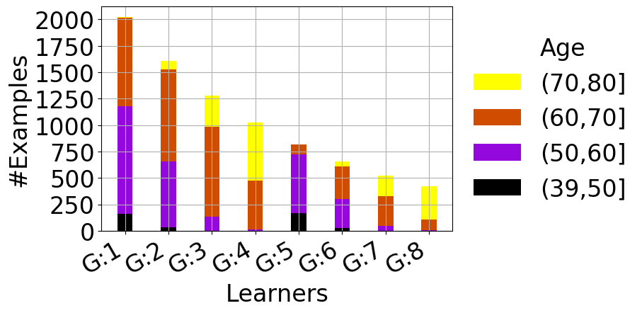
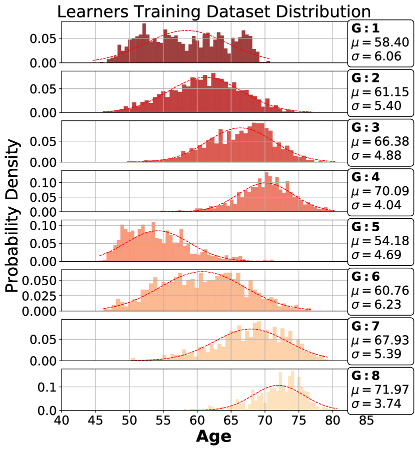
For the statistical heterogeneity of the regression task in BrainAge, we partition (following (Stripelis et al., 2021a)) the UKBB neuroimaging dataset (Miller et al., 2016) into training (8356 records) and test (2090 records) across a federation of 8 learners with skewed data amounts, and IID and Non-IID age distributions. In the IID case, every learner holds data examples from all possible age ranges, while in the Non-IID case learners hold examples from a subset of age ranges. Figure 6 shows the distribution of the training examples across the 8 learners over three different learning environments in BrainAge. Every environment is evaluated on the same test dataset representative of the global age distribution.
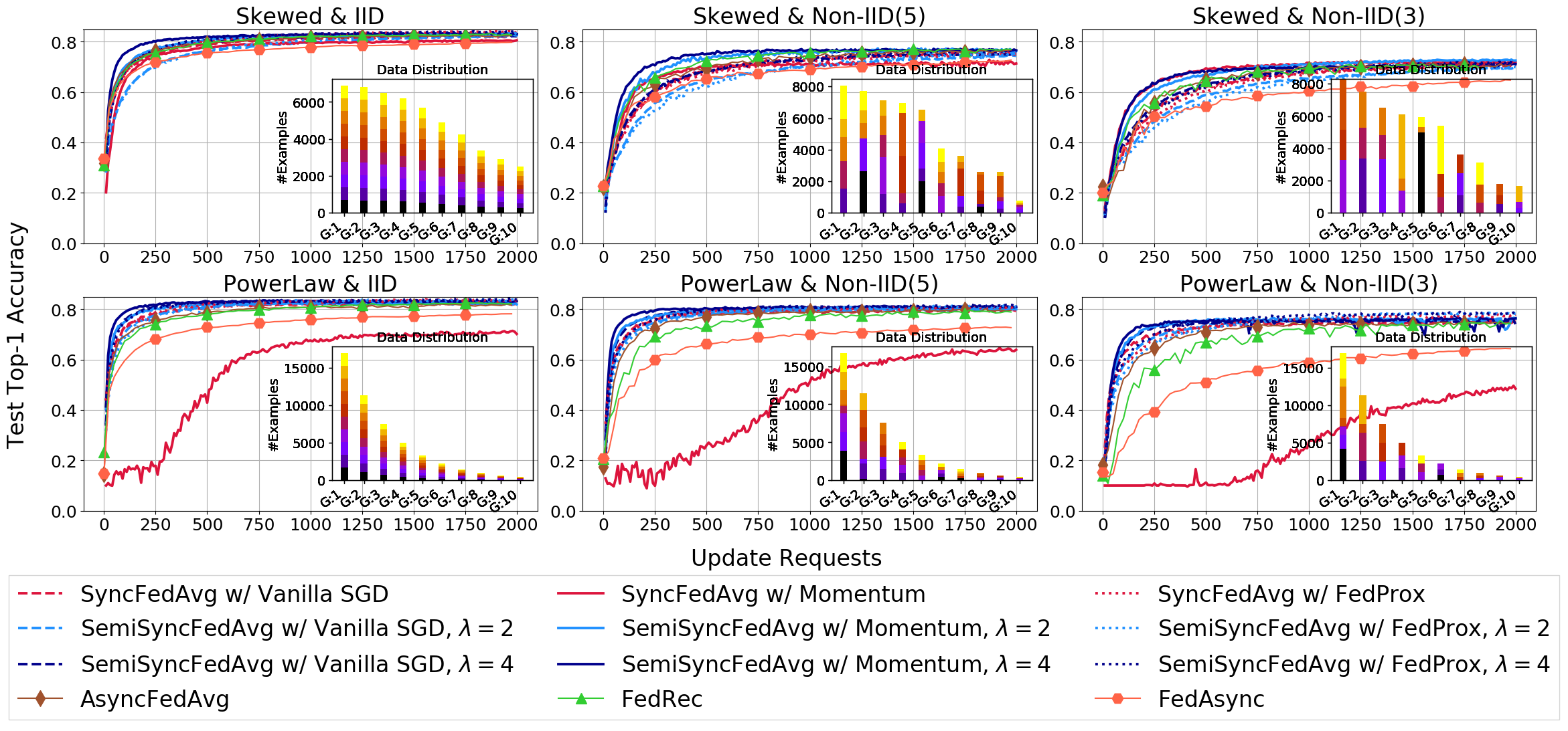
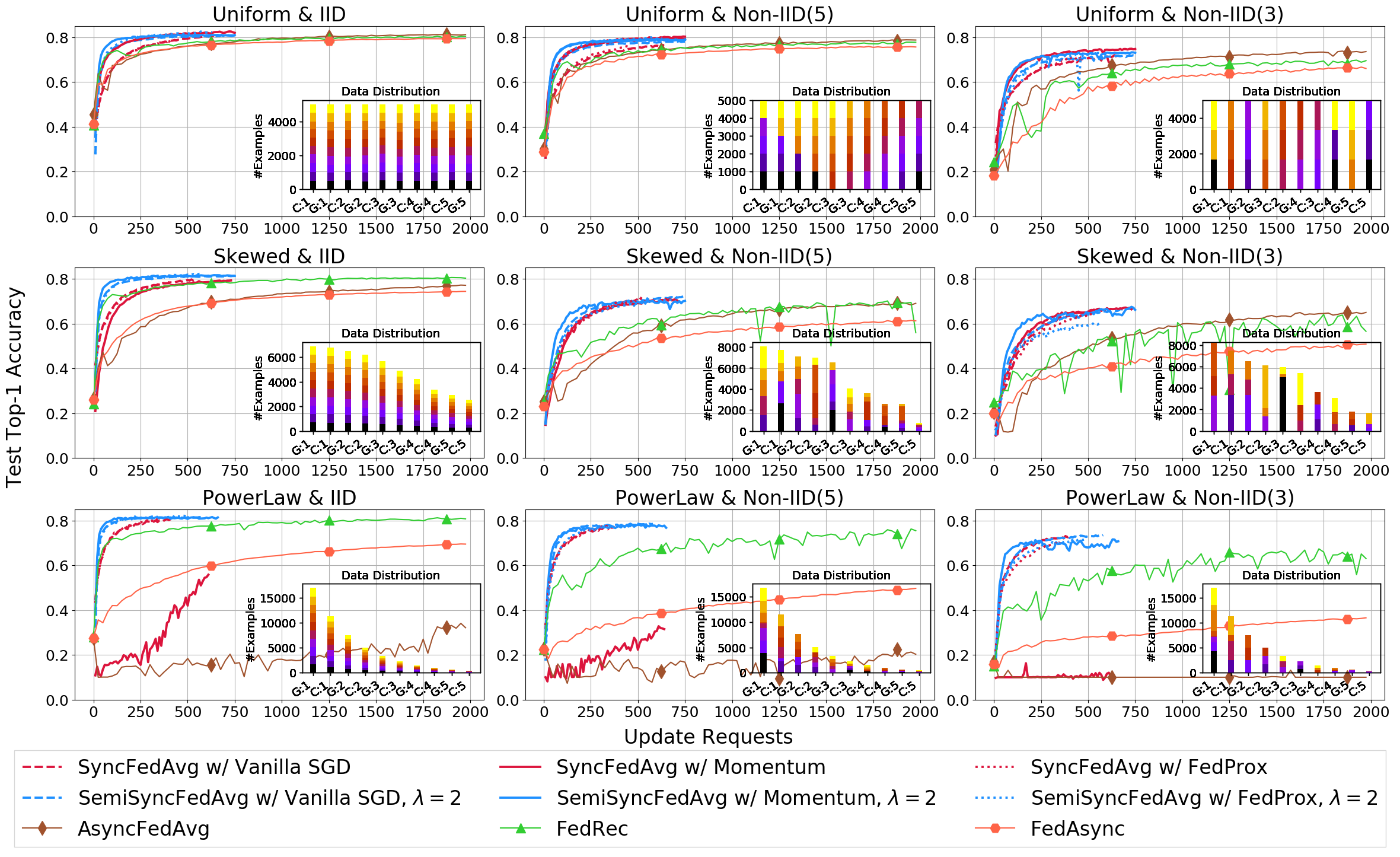
Within each learning domain, all training policies were run for the same amount of wall-clock time. In homogeneous computational environments (cf. Figure 7(b)), the total number of update requests for synchronous and asynchronous policies is similar, since any latency occurs only due to differences in the amount of training data. However, in heterogeneous computational environments, during asynchronous training, computationally fast learners issue many more update requests than slow learners. In synchronous and semi-synchronous policies, the update requests are substantially smaller and driven by the slowest learner in the federation. To highlight the differences in communication costs, Figures 8(b), 9(b) and 10(b) show the number of update requests issued by all learners for the same wall-clock time period (set in Figures 8(a), 9(a) and 10(a), respectively). Point markers in the asynchronous policies are just a visual aid to distinguish them from synchronous and semi-synchronous policies.
CIFAR-10 Results
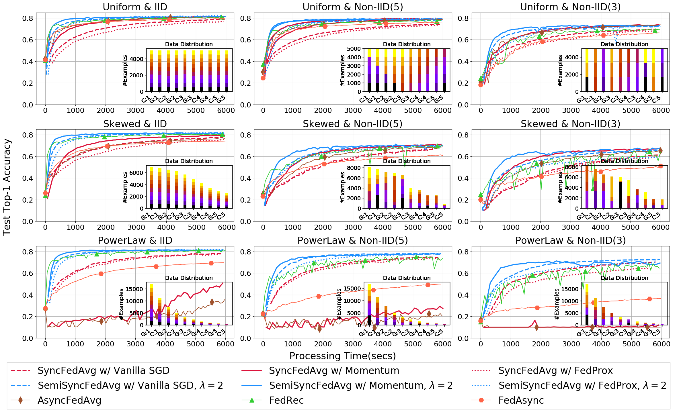
Figure 7 shows the performance of synchronous, semi-synchronous, and asynchronous policies in a homogeneous computational environment, where all learners have the same computational capabilities (10 GPUs). We compare the different policies on heterogeneous amounts of data per learner (Skewed, Power Law) since for a homogeneous computational environment with an equal number of data points (Uniform) across learners, all policies are equivalent. For the synchronous policies, idle time still occurs due to the different data amount in the Skewed and Power Law data distributions. For SemiSync and asynchronous policies, there is no idle time. We evaluate SyncFedAvg and SemiSyncFedAvg with Vanilla SGD, Momemtum SGD, and FedProx, and AsyncFedAvg, FedRec, and FedAsync with MomentumSGD. SyncFedAvg with Momentum converges very slowly in Power Law data distributions, but using FedProx as a local optimizer rescues it. SemiSync with Momentum and results in the fastest convergence across the experiments in Figure 7(a) (see also Table 2). Similar results hold for communication cost in terms of update requests as shown in Figure 7(b). When the amounts of data across learners is not too great (Skewed data distributions) AsyncFedAvg and FedRec have comparable performance, but as the difference in data increases (PowerLaw data distributions), AsyncFedAvg is more efficient compared to the staleness-aware weighting scheme of both FedRec and FedAsync.
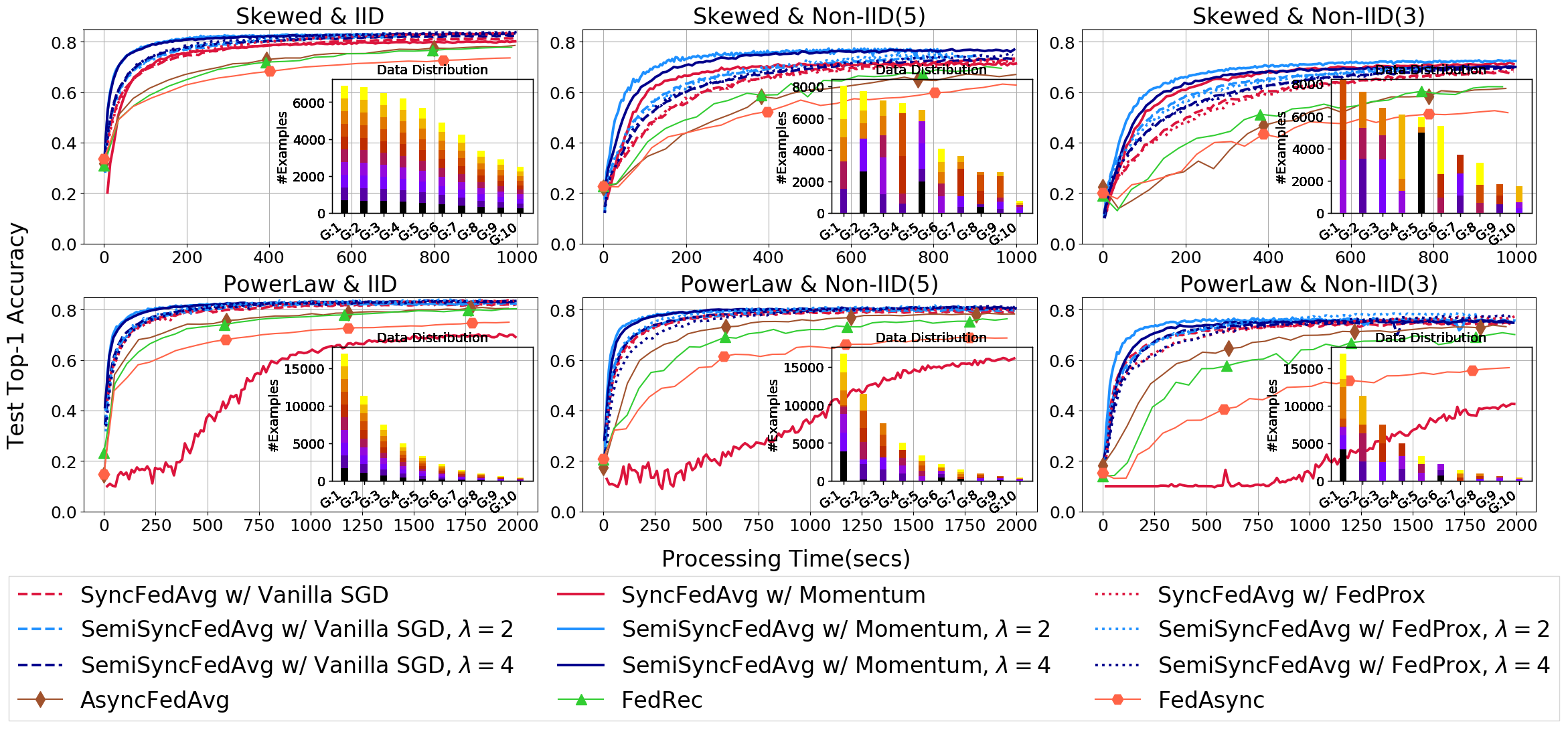
Figure 8 shows the performance on the CIFAR-10 domain of synchronous, asynchronous, and semi-synchronous policies in a heterogeneous computational environment (with 10 learners: 5 fast GPUs, and 5 slow CPUs; the CPUs’ batch processing is 10 times slower than the GPUs). Again, our SemiSync with Momentum () has the best performance with faster convergence (some other policies reach comparable accuracy levels eventually). As we move towards more challenging Non-IID learning environments, all methods show a reduction in the final performance (lower accuracy). SyncFedAvg with Momentum performs reasonably well with moderate levels of data heterogeneity (Skewed data amounts, with either IID or Non-IID distributions). However, in more extreme data distributions (Power Law), it learns very slowly, since the local models are more disparate and the momentum factor limits changes to the community model. In SemiSync the fast learners perform more local iterations and mix more frequently, which facilitates the convergence of the federation even for the same momentum factor that slowed learning for SyncFedAvg. This is exarcerbated in the heterogeneous case, compared to the homogeneous case, since the training speed differences are much greater. Interestingly, SyncFedAvg with FedProx performs much better in these cases, although still worse than the SemiSync policies. FedRec dominates other asynchronous policies on convergence rate, especially in IID environments and in Power Law distributions. In Uniform and Skewed Non-IID environments, its performance is comparable to AsyncFedAvg. Comparing the experiments based on data amounts, we can see that in some learning environments, such as Skewed & Non-IID(5) and Power Law & Non-IID(5) in Figures 7 and 8, the optimal accuracy is higher in the Power Law case compared to its Skewed counterpart. This is due to the fact that the head (G:1) of the Power Law distribution covers most of the domain data (8 classes) and therefore its local model is more valuable and has a greater contribution value in the community model.
The communication cost of SemiSync policies is comparable to synchronous policies reaching a high accuracy very quickly, while asynchronous policies require many more update requests to achieve the same (or worse) level of accuracy (Figure 8(b)). For Power Law data distributions SyncFedAvg with Momentum fails to learn, but SyncFedAvg with FedProx learns and efficiently uses communication. Similar to the homogeneous case, our semi-synchronous policies dominate in heterogeneous environments (see also Table 3).
CIFAR-100 Results
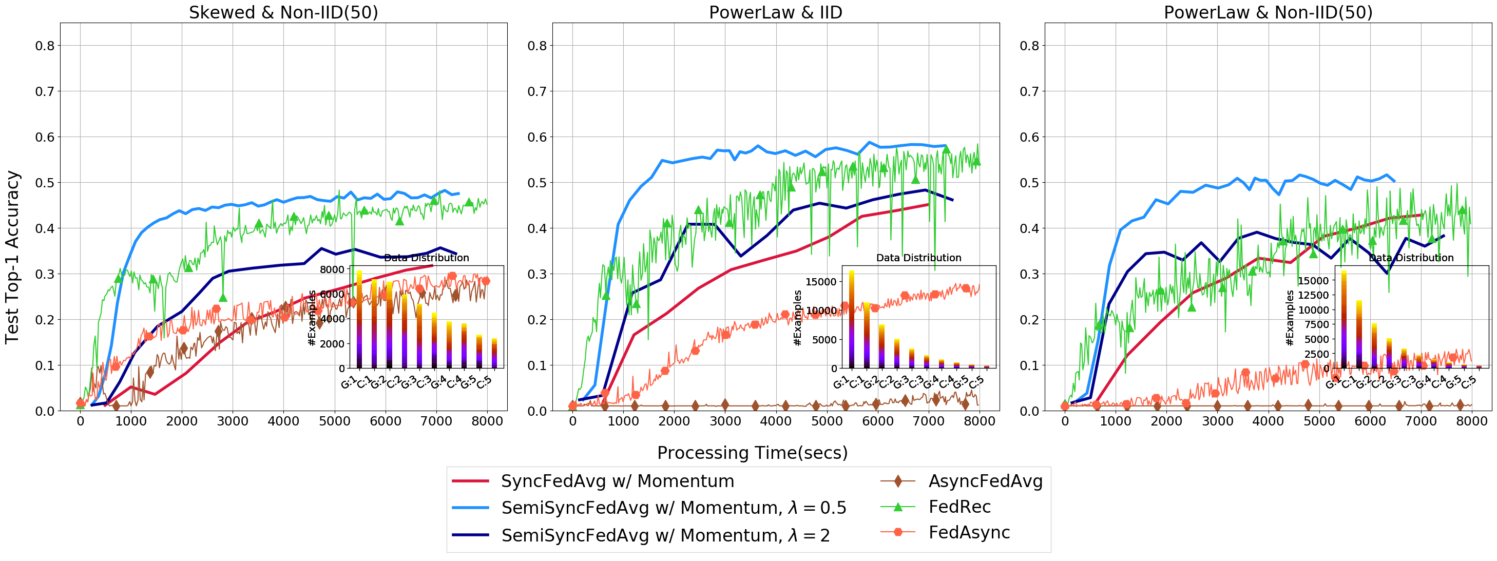
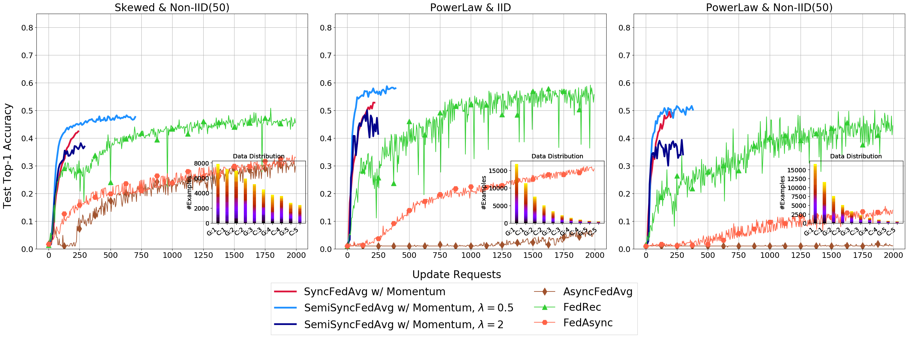
Figure 9 shows the performance on the CIFAR-100 domain of synchronous, asynchronous, and semi-synchronous policies in a heterogeneous computational environment (with 10 learners: 5 fast GPUs, and 5 slow CPUs). Due to the size and computational complexity of the ResNet-50 model used to train on the CIFAR-100 domain, the performance difference between fast and slow learners is large (CPUs batch processing is 33 times slower than the GPUs). Using a smaller value of leads to better results for the SemiSync policy. We use , which means that the slowest learner processes only half of its local dataset at each SemiSync synchronization point. However, since the batches are chosen randomly, after two synchronization points all the data is processed (on average). FedRec dominates alternative asynchronous policies, though is less stable. Our SemiSync with Momentum () policy yields the fastest convergence rate and final accuracy, while remaining communication efficient.
ExtendedMNIST Results
Figure 10 shows the results on the ExtendedMNIST By Class domain on heterogeneous environments (10 learners: 5 fast, 5 slow; slow learners (CPUs) are 16 times slower than fast learners (GPUs)). Extended MNIST By Class is a very challenging learning task due to its unbalanced distribution of target classes and large amount of data samples (731,668 training examples). As we empirically show, SemiSync performs considerably better compared to other policies both in terms of convergence speed and in terms of communication cost. Among the asynchronous policies, FedRec has faster convergence and better generalization. Interestingly, asynchronous policies have faster convergence at the beginning of the federated training, a behavior that is more pronounced for FedRec in the Power Law & IID environment. Given the large number of records allocated to the slow learners (e.g., C:1 owns 90,000 in Skewed and 140,000 examples in Power Law), the total processing time required to complete their local training task is much higher compared to fast. Moreover, since in asynchronous policies no idle time exists for the fast learners, the convergence of the community model is driven by their learning pace and more frequent communication, whereas in synchronous and semi-synchronous all learners need to complete their local training task before a new community model is computed; hence the delayed convergence of Sync and SemiSync at the start of training.
BrainAge Results
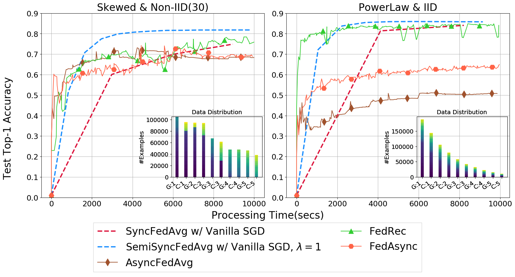
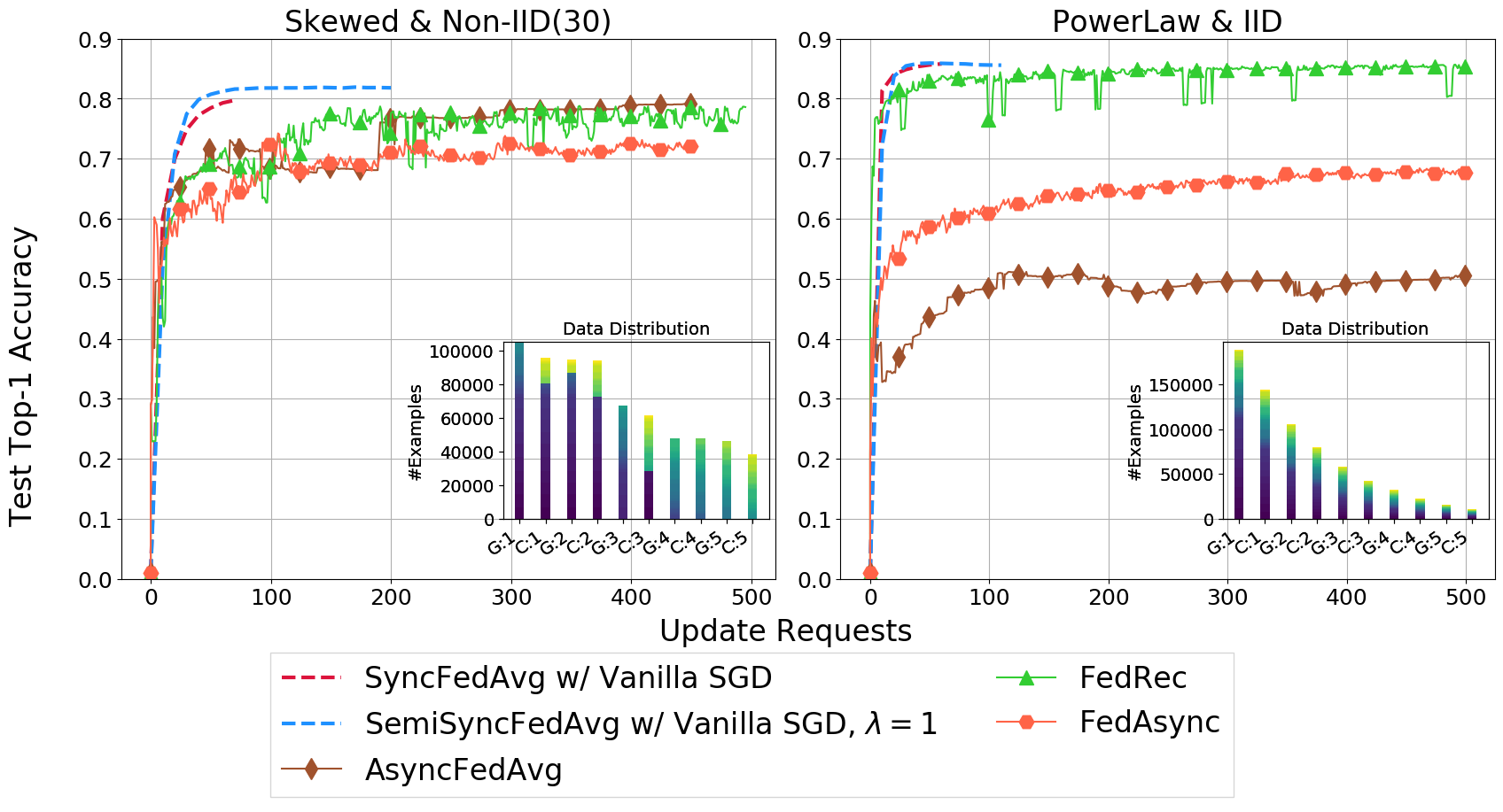
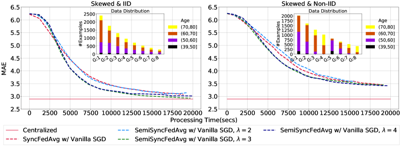
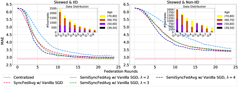
We evaluate the synchronous and SemiSync policies on a computationally homogeneous environment with Skewed IID and Non-IID data distributions (for Uniform data amounts both policies behave identically, see (Stripelis et al., 2021a) for results in this environment) on the BrainAge domain. In terms of parallel processing time, SemiSync with provides faster convergence for both Skewed IID and Non-IID distributions compared to the synchronous policy. In terms of communication cost, SemiSync with is more communication efficient for both data distributions, with being comparable to synchronous. For IID, SemiSync with leads to the smallest mean absolute error, which is very close to the error reached by the centralized model.
Models Performance: Time, Communication, and Energy
We analyze the performance of the different federated training policies in terms of time, communication,666We disregard model transmission costs. In heterogeneous environments for CIFAR-10, CIFAR-100 and ExtendedMNIST, the model size, average model transmission time, average processing time for SemiSync, and ratio of model transmission to computation are: (4MB, 0.4secs, 80secs , 0.005), (5MB, 0.4secs, 80secs , 0.003), and (50MB, 5secs, 1000secs , 0.005), respectively. Similarly, for the homogeneous environment of BrainAge we have (11MB, 0.9secs, 850secs , 0.001). and energy costs, in the CIFAR-10 domain in both homogeneous (Table 2) and heterogeneous (Table 3) environments. To compare the training policies, we pick a target accuracy that can be reached by (most of) the policies and calculate the different metrics as defined in Section 4.4. To compute the energy cost in the heterogeneous computational environment, we set for GPUs and for CPUs (see eq. 8). Since estimating the full energy consumption (network, storage, power conversion) is challenging, we compute the energy cost ratio between GPUs and CPUs based on their Thermal Design Power (TDP) value (Dayarathna et al., 2015), which accounts for the maximum amount of heat generated by a processor. For the GPU GeForce GTX 1080 Ti the TDP value is 180W, while for the Intel(R) Xeon(R) CPU the TDP value is 90W. In both homogeneous and heterogeneous domains, SemiSync with Momentum () performs best in terms of the (parallel/wall-clock) time to reach the desired target accuracy and in terms of the energy cost (with depends on the cumulative processing time across all learners needed to reach that accuracy). In heterogeneous domains, SemiSync with Momentum () is also the most efficient in terms of communication. In homogeneous domains SemiSync with Momentum () is more communication efficient, but with slightly slower convergence and larger energy cost, when compared to (). Remarkably, when our SemiSync strategy is combined with any local optimizer and compared to its synchronous counterpart, it yields significant energy savings close to an average 40% energy cost reduction in both homogeneous and heterogeneous computational environments (cf. Tables 2 and 3). Finally, comparing the performance of the different local optimizers, Momentum SGD provides accelerated convergence with a lower communication overhead compared to Vanilla SGD and FedProx. At the same time Momentum SGD is the most energy-efficient policy, compared to the Synchronous Vanilla SGD baseline, with a reduction of 3 to 9 times the energy cost.
|
|
|
|
|
|
|
|||||||||||
|---|---|---|---|---|---|---|---|---|---|---|---|---|---|---|---|---|---|
| Skewed & Non-IID(5) 0.7 | Sync w/ Vanilla | 123220 | 613 | 6133 | 610 | 12267 | |||||||||||
| SemiSync () w/ Vanilla | 156025 | 444 | 3541 | 970 | 7083 (1.7x) | ||||||||||||
| SemiSync () w/ Vanilla | 201385 | 551 | 4507 | 630 | 9014 (1.3x) | ||||||||||||
| Sync w/ Momentum | 92920 | 319 | 3190 | 460 | 6381 (1.9x) | ||||||||||||
| SemiSync () w/ Momentum | 47485 | 121 | 1005 | 300 | 2010 (6.1x) | ||||||||||||
| SemiSync () w/ Momentum | 58825 | 161 | 1324 | 190 | 2648 (4.6x) | ||||||||||||
| Sync w/ FedProx | 135340 | 630 | 6305 | 670 | 12610 (0.9x) | ||||||||||||
| SemiSync () w/ FedProx | 144685 | 380 | 3134 | 900 | 6268 (1.9x) | ||||||||||||
| SemiSync () w/ FedProx | 185185 | 481 | 3876 | 580 | 7752 (1.5x) | ||||||||||||
| FedRec | 61224 | 924 | 3830 | 358 | 7661 (1.6x) | ||||||||||||
| AsyncFedAvg | 78098 | 1166 | 4864 | 456 | 9729 (1.2x) | ||||||||||||
| FedAsync | 198990 | 3120 | 12709 | 1164 | 25419 (0.4x) | ||||||||||||
| Power Law & Non-IID(3) 0.65 | Sync w/ Vanilla | 24240 | 181 | 1811 | 120 | 3623 | |||||||||||
| SemiSync () w/ Vanilla | 54905 | 199 | 1347 | 170 | 2695 (1.3x) | ||||||||||||
| SemiSync () w/ Vanilla | 68505 | 208 | 1694 | 110 | 3389 (1.1x) | ||||||||||||
| Sync w/ Momentum | did not reach target accuracy | ||||||||||||||||
| SemiSync () w/ Momentum | 31105 | 86 | 667 | 100 | 1335 (2.7x) | ||||||||||||
| SemiSync () w/ Momentum | 48105 | 146 | 1181 | 80 | 2363 (1.5x) | ||||||||||||
| Sync w/ FedProx | 38380 | 287 | 2876 | 190 | 5752 | ||||||||||||
| SemiSync () w/ FedProx | 75305 | 208 | 1620 | 230 | 3241 (1.1x) | ||||||||||||
| SemiSync () w/ FedProx | 95705 | 291 | 2157 | 150 | 4315 (0.8x) | ||||||||||||
| FedRec | 45822 | 877 | 3360 | 365 | 6720 (0.5x) | ||||||||||||
| AsyncFedAvg | 30894 | 609 | 2357 | 255 | 4715 (0.7x) | ||||||||||||
| FedAsync | 247068 | 4727 | 18165 | 1981 | 36331 (0.1x) | ||||||||||||
|
|
|
|||||||||||||||||||||||
|
|
|
|
|
|
|
|
|
|
|
|
|
|||||||||||||
| Uniform & IID 0.75 | Sync w/ Vanilla | 24000 | 578 | 1157 | 24000 | 16129 | 16129 | 48000 | 3225 | 16707 | 240 | 17286 | |||||||||||||
| SemiSync () w/ Vanilla | 45250 | 1018 | 2036 | 4750 | 3045 | 3045 | 50000 | 631 | 4064 | 100 | 5082 (3.4x) | ||||||||||||||
| Sync w/ Momentum | 11000 | 185 | 371 | 11000 | 2700 | 2700 | 22000 | 540 | 2885 | 110 | 3071 (5.6x) | ||||||||||||||
| SemiSync () w/ Momentum | 20250 | 335 | 671 | 2250 | 1217 | 1217 | 22500 | 269 | 1553 | 50 | 1889 (9.1x) | ||||||||||||||
| Sync w/ FedProx | 24000 | 548 | 1097 | 24000 | 22015 | 22015 | 48000 | 4403 | 22564 | 240 | 23113 (0.7x) | ||||||||||||||
| SemiSync () w/ FedProx | 40250 | 817 | 1634 | 4250 | 4074 | 4074 | 44500 | 928 | 4891 | 90 | 5708 (3x) | ||||||||||||||
| FedRec | 50800 | 1588 | 3177 | 1600 | 1449 | 1449 | 52400 | 732 | 3038 | 261 | 4627 (3.7x) | ||||||||||||||
| AsyncFedAvg | 69200 | 2439 | 4879 | 8800 | 2870 | 2870 | 78000 | 1315 | 5310 | 389 | 7750 (2.2x) | ||||||||||||||
| FedAsync | 76600 | 2703 | 5406 | 8000 | 3147 | 3147 | 84600 | 1406 | 5850 | 422 | 8554 (2x) | ||||||||||||||
| Skewed & Non-IID(5) 0.65 | Sync w/ Vanilla | 28200 | 1010 | 2020 | 22300 | 22812 | 22812 | 50500 | 4562 | 23822 | 250 | 24832 | |||||||||||||
| SemiSync () w/ Vanilla | 164082 | 3585 | 7170 | 16603 | 10006 | 10006 | 180685 | 2153 | 13591 | 220 | 17176 (1.4x) | ||||||||||||||
| Sync w/ Momentum | 28200 | 670 | 1341 | 22300 | 10896 | 10896 | 50500 | 2179 | 11567 | 250 | 12238 (2x) | ||||||||||||||
| SemiSync () w/ Momentum | 93882 | 1446 | 2893 | 9583 | 4434 | 4434 | 103465 | 1059 | 5881 | 130 | 7328 (3.3x) | ||||||||||||||
| Sync w/ FedProx | 29328 | 1065 | 2130 | 23192 | 22998 | 22998 | 52520 | 4599 | 24063 | 260 | 25129 (0.9x) | ||||||||||||||
| SemiSync () w/ FedProx | 210882 | 4677 | 9354 | 21283 | 12872 | 12872 | 232165 | 2884 | 17549 | 280 | 22226 (1.1x) | ||||||||||||||
| FedRec | 155731 | 5205 | 10411 | 4378 | 4448 | 4448 | 160109 | 2431 | 9654 | 803 | 14860 (1.6x) | ||||||||||||||
| AsyncFedAvg | 183982 | 6185 | 12370 | 17361 | 7349 | 7349 | 201343 | 3346 | 13534 | 1021 | 19719 (1.2x) | ||||||||||||||
| FedAsync | did not reach target accuracy | ||||||||||||||||||||||||
| Power Law & Non-IID(3) 0.6 | Sync w/ Vanilla | 9664 | 600 | 1201 | 6496 | 10107 | 10107 | 16160 | 2021 | 10707 | 80 | 11308 | |||||||||||||
| SemiSync () w/ Vanilla | 80102 | 1831 | 3662 | 8183 | 4939 | 4939 | 88285 | 1103 | 6770 | 80 | 8601 (1.3x) | ||||||||||||||
| Sync w/ Momentum | did not reach target accuracy | ||||||||||||||||||||||||
| SemiSync () w/ Momentum | 34502 | 573 | 1147 | 3623 | 1723 | 1723 | 38125 | 438 | 2296 | 40 | 2870 (3.9x) | ||||||||||||||
| Sync w/ FedProx | 13288 | 863 | 1727 | 8932 | 16363 | 16363 | 22220 | 3272 | 17227 | 110 | 18091 (0.6x) | ||||||||||||||
| SemiSync () w/ FedProx | 102902 | 2084 | 4168 | 10463 | 7084 | 7084 | 113365 | 1719 | 9168 | 100 | 11252 (1x) | ||||||||||||||
| FedRec | 90458 | 3671 | 7343 | 2647 | 2922 | 2922 | 93105 | 1832 | 6594 | 664 | 10266 (1.1x) | ||||||||||||||
| AsyncFedAvg | did not reach target accuracy | ||||||||||||||||||||||||
| FedAsync | did not reach target accuracy | ||||||||||||||||||||||||
The Case for Federated Learning.
Federated Learning is an efficient distributed machine learning paradigm that can allow multiple learning sites (learners) to jointly train a machine learning model without the need to share data (i.e., move the data out of their original source to a central site). This is critical in many domains, particularly in health informatics and in biomedical/genetics research consortia, where it is hard to share data due to privacy protections.
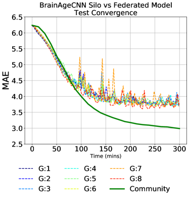
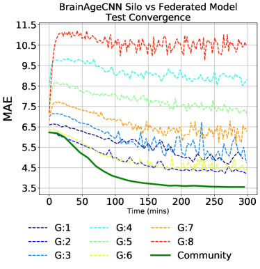
To demonstrate the benefits of Federated Learning in a realistic biomedical domain, we analyzed the performance of individual sites training on their local data versus training in a federation for the BrainAge domain under different data distributions. Figure 12(a) considers an Uniform & IID environment, where each site has the same amount of data and full representation of age ranges (cf. Figure6(a,b)). Even in this benign environment, the community model obtained by the federation significantly outperforms the model achieved by any single site. Figure 12(b) considers a Skewed & Non-IID environment, where different sites have different amounts of data and different age distributions (cf. Figure6(c,d)). This more realistic scenario would be typical of research consortia or federation of hospitals and clinics of different sizes and different disease prevalence. In this case, sites with smaller datasets or data distributions farther from the global distribution show very poor performance. Again, even the sites with larger datasets cannot match the community model. In summary, sites both small and large have strong incentives to join in Federated Learning.
7. Discussion
We have presented a novel Semi-Synchronous Federated Learning training policy, SemiSync, with fast convergence and low communication and energy costs, particularly in heterogeneous data and computational environments. SemiSync defines a synchronization time point where all learners share their current local model to compute the community model. Compared to synchronous policies, learners with different amounts of data and/or computational power do not remain idle. By choosing the synchronization point so that the amount of data processed by the learners does not become too dissimilar, we can achieve faster convergence without increasing communication costs and with less energy consumption. We performed extensive experiments comparing synchronous (FedAvg), asynchronous (FedAsync, FedRec), and semi-synchronous (SemiSync) policies in heterogeneous data and computational environments on standard benchmarks and on a challenging neuroimaging domain. We show experimentally that our SemiSync policy provides accelerated convergence and reaches better or comparable eventual accuracy than previous approaches. The effects are more pronounced the more challenging the domain is, such as the results on CIFAR-100 and BrainAge with different data amounts per learner and Non-IID distributions.
In future work, we plan to explore (1) adaptive hyperparameter (e.g., , ) schedules, (2) server-side model optimization update rules (Reddi et al., 2020; Wang et al., 2021; Hsu et al., 2019), and (3) federated learning policies under different homomorphic encryption schemes (Stripelis et al., 2021b). We also plan to adapt the SemiSync protocol to cross-device settings by considering connectivity and bandwidth limitations, and estimating hyperparameter lambda from a sample of learners and progressively fine-tuning it as more learners are sampled.
Acknowledgements.
This research was supported in part by the Defense Advanced Research Projects Activity (DARPA) under contract HR00112090104, and in part by the National Institutes of Health (NIH) under grants U01AG068057 and RF1AG051710. The views and conclusions contained herein are those of the authors and should not be interpreted as necessarily representing the official policies or endorsements, either expressed or implied, of DARPA, NIH, or the U.S. Government. This is a study of previously collected, anonymized, de-identified data, available in a public repository. Data access approved by UK Biobank under Application Number 11559.References
- (1)
- Abadi et al. (2016a) Martín Abadi, Paul Barham, Jianmin Chen, Zhifeng Chen, Andy Davis, Jeffrey Dean, Matthieu Devin, Sanjay Ghemawat, Geoffrey Irving, Michael Isard, et al. 2016a. Tensorflow: A system for large-scale machine learning. In 12th USENIX Symposium on Operating Systems Design and Implementation (OSDI 16). 265–283.
- Abadi et al. (2016b) Martin Abadi, Andy Chu, Ian Goodfellow, H Brendan McMahan, Ilya Mironov, Kunal Talwar, and Li Zhang. 2016b. Deep learning with differential privacy. In Proceedings of the 2016 ACM SIGSAC Conference on Computer and Communications Security. 308–318.
- Agarwal and Duchi (2011) Alekh Agarwal and John C Duchi. 2011. Distributed delayed stochastic optimization. In Advances in Neural Information Processing Systems. 873–881.
- Bellavista et al. (2021) Paolo Bellavista, Luca Foschini, and Alessio Mora. 2021. Decentralised learning in federated deployment environments: A system-level survey. ACM Computing Surveys (CSUR) 54, 1 (2021), 1–38.
- Bertsekas (1983) Dimitri P Bertsekas. 1983. Distributed asynchronous computation of fixed points. Mathematical Programming 27, 1 (1983), 107–120.
- Bertsekas and Tsitsiklis (1989) Dimitri P Bertsekas and John N Tsitsiklis. 1989. Parallel and distributed computation: numerical methods. Vol. 23. Prentice hall Englewood Cliffs, NJ.
- Bonawitz et al. (2019) Keith Bonawitz, Hubert Eichner, Wolfgang Grieskamp, Dzmitry Huba, Alex Ingerman, Vladimir Ivanov, Chloé Kiddon, Jakub Konečný, Stefano Mazzocchi, Brendan McMahan, Timon Van Overveldt, David Petrou, Daniel Ramage, and Jason Roselander. 2019. Towards Federated Learning at Scale: System Design. In Proceedings of Machine Learning and Systems, A. Talwalkar, V. Smith, and M. Zaharia (Eds.), Vol. 1. 374–388.
- Bonawitz et al. (2017) Keith Bonawitz, Vladimir Ivanov, Ben Kreuter, Antonio Marcedone, H Brendan McMahan, Sarvar Patel, Daniel Ramage, Aaron Segal, and Karn Seth. 2017. Practical secure aggregation for privacy-preserving machine learning. In proceedings of the 2017 ACM SIGSAC Conference on Computer and Communications Security. ACM, 1175–1191.
- Caldas et al. (2018) Sebastian Caldas, Peter Wu, Tian Li, Jakub Konečnỳ, H Brendan McMahan, Virginia Smith, and Ameet Talwalkar. 2018. Leaf: A benchmark for federated settings. arXiv preprint arXiv:1812.01097 (2018).
- Chai et al. (2020) Zheng Chai, Ahsan Ali, Syed Zawad, Stacey Truex, Ali Anwar, Nathalie Baracaldo, Yi Zhou, Heiko Ludwig, Feng Yan, and Yue Cheng. 2020. Tifl: A tier-based federated learning system. In Proceedings of the 29th International Symposium on High-Performance Parallel and Distributed Computing. 125–136.
- Chen et al. (2016) Jianmin Chen, Xinghao Pan, Rajat Monga, Samy Bengio, and Rafal Jozefowicz. 2016. Revisiting distributed synchronous SGD. arXiv preprint arXiv:1604.00981 (2016).
- Chen et al. (2020) Mingzhe Chen, Zhaohui Yang, Walid Saad, Changchuan Yin, H Vincent Poor, and Shuguang Cui. 2020. A joint learning and communications framework for federated learning over wireless networks. IEEE Transactions on Wireless Communications 20, 1 (2020), 269–283.
- Cohen et al. (2017) Gregory Cohen, Saeed Afshar, Jonathan Tapson, and Andre Van Schaik. 2017. EMNIST: Extending MNIST to handwritten letters. In 2017 International Joint Conference on Neural Networks (IJCNN). IEEE, 2921–2926.
- Cole et al. (2017) James H Cole, Rudra PK Poudel, Dimosthenis Tsagkrasoulis, Matthan WA Caan, Claire Steves, Tim D Spector, and Giovanni Montana. 2017. Predicting brain age with deep learning from raw imaging data results in a reliable and heritable biomarker. NeuroImage 163 (2017), 115–124.
- Cui et al. (2014) Henggang Cui, James Cipar, Qirong Ho, Jin Kyu Kim, Seunghak Lee, Abhimanu Kumar, Jinliang Wei, Wei Dai, Gregory R Ganger, Phillip B Gibbons, et al. 2014. Exploiting bounded staleness to speed up big data analytics. In 2014 USENIX Annual Technical Conference (USENIXATC 14). 37–48.
- Dai (2018) Wei Dai. 2018. Learning with Staleness. Ph.D. Dissertation. Carnegie Mellon University.
- Dai et al. (2019) Wei Dai, Yi Zhou, Nanqing Dong, Hao Zhang, and Eric Xing. 2019. Toward Understanding the Impact of Staleness in Distributed Machine Learning. In International Conference on Learning Representations.
- Dayarathna et al. (2015) Miyuru Dayarathna, Yonggang Wen, and Rui Fan. 2015. Data center energy consumption modeling: A survey. IEEE Communications Surveys & Tutorials 18, 1 (2015), 732–794.
- Dean and Barroso (2013) Jeffrey Dean and Luiz André Barroso. 2013. The tail at scale. Commun. ACM 56, 2 (2013), 74–80.
- Dean et al. (2012) Jeffrey Dean, Greg Corrado, Rajat Monga, Kai Chen, Matthieu Devin, Mark Mao, Marc’aurelio Ranzato, Andrew Senior, Paul Tucker, Ke Yang, et al. 2012. Large scale distributed deep networks. In Advances in neural information processing systems. 1223–1231.
- Gao et al. (2020) Zhifan Gao, Heye Zhang, Shizhou Dong, Shanhui Sun, Xin Wang, Guang Yang, Wanqing Wu, Shuo Li, and Victor Hugo C de Albuquerque. 2020. Salient object detection in the distributed cloud-edge intelligent network. IEEE Network 34, 2 (2020), 216–224.
- Gupta et al. (2021) Umang Gupta, Pradeep Lam, Greg Ver Steeg, and Paul Thompson. 2021. Improved Brain Age Estimation with Slice-based Set Networks. In IEEE International Symposium on Biomedical Imaging (ISBI).
- Hauswirth and Jazayeri (1999) Manfred Hauswirth and Mehdi Jazayeri. 1999. A component and communication model for push systems. In Software Engineering—ESEC/FSE’99. Springer, 20–38.
- Herlihy and Wing (1990) Maurice P Herlihy and Jeannette M Wing. 1990. Linearizability: A correctness condition for concurrent objects. ACM Transactions on Programming Languages and Systems (TOPLAS) 12, 3 (1990), 463–492.
- Ho et al. (2013) Qirong Ho, James Cipar, Henggang Cui, Seunghak Lee, Jin Kyu Kim, Phillip B Gibbons, Garth A Gibson, Greg Ganger, and Eric P Xing. 2013. More effective distributed ml via a stale synchronous parallel parameter server. In Advances in neural information processing systems. 1223–1231.
- Hsu et al. (2019) Tzu-Ming Harry Hsu, Hang Qi, and Matthew Brown. 2019. Measuring the effects of non-identical data distribution for federated visual classification. arXiv preprint arXiv:1909.06335 (2019).
- Jain (2003) Ramesh Jain. 2003. Out-of-the-box data engineering events in heterogeneous data environments. In Proceedings 19th International Conference on Data Engineering (Cat. No. 03CH37405). IEEE, 8–21.
- Jónsson et al. (2019) Benedikt Atli Jónsson, Gyda Bjornsdottir, TE Thorgeirsson, Lotta María Ellingsen, G Bragi Walters, DF Gudbjartsson, Hreinn Stefansson, Kari Stefansson, and MO Ulfarsson. 2019. Brain age prediction using deep learning uncovers associated sequence variants. Nature communications 10, 1 (2019), 1–10.
- Kairouz and McMahan (2021) Peter Kairouz and H. Brendan McMahan. 2021. Advances and Open Problems in Federated Learning. Foundations and Trends® in Machine Learning 14, 1 (2021), –. https://doi.org/10.1561/2200000083
- Kilbertus et al. (2018) Niki Kilbertus, Adrià Gascón, Matt J Kusner, Michael Veale, Krishna P Gummadi, and Adrian Weller. 2018. Blind justice: Fairness with encrypted sensitive attributes. arXiv preprint arXiv:1806.03281 (2018).
- Kim et al. (2017) Yejin Kim, Jimeng Sun, Hwanjo Yu, and Xiaoqian Jiang. 2017. Federated tensor factorization for computational phenotyping. In Proceedings of the 23rd ACM SIGKDD International Conference on Knowledge Discovery and Data Mining. 887–895.
- Konečnỳ et al. (2016) Jakub Konečnỳ, H Brendan McMahan, Felix X Yu, Peter Richtárik, Ananda Theertha Suresh, and Dave Bacon. 2016. Federated learning: Strategies for improving communication efficiency. arXiv preprint arXiv:1610.05492 (2016).
- Lamport (1979) Leslie Lamport. 1979. How to make a multiprocessor computer that correctly executes multiprocess progranm. IEEE transactions on computers 28, 9 (1979), 690–691.
- Lee et al. (2018) Junghye Lee, Jimeng Sun, Fei Wang, Shuang Wang, Chi-Hyuck Jun, and Xiaoqian Jiang. 2018. Privacy-preserving patient similarity learning in a federated environment: development and analysis. JMIR medical informatics 6, 2 (2018).
- Li et al. (2020c) Tian Li, Anit Kumar Sahu, Ameet Talwalkar, and Virginia Smith. 2020c. Federated learning: Challenges, methods, and future directions. IEEE Signal Processing Magazine 37, 3 (2020), 50–60.
- Li et al. (2020d) Tian Li, Anit Kumar Sahu, Manzil Zaheer, Maziar Sanjabi, Ameet Talwalkar, and Virginia Smith. 2020d. Federated Optimization in Heterogeneous Networks. In Proceedings of Machine Learning and Systems, I. Dhillon, D. Papailiopoulos, and V. Sze (Eds.), Vol. 2. 429–450. https://proceedings.mlsys.org/paper/2020/file/38af86134b65d0f10fe33d30dd76442e-Paper.pdf
- Li et al. (2019) Wenqi Li, Fausto Milletarì, Daguang Xu, Nicola Rieke, Jonny Hancox, Wentao Zhu, Maximilian Baust, Yan Cheng, Sébastien Ourselin, M Jorge Cardoso, et al. 2019. Privacy-preserving federated brain tumour segmentation. In International Workshop on Machine Learning in Medical Imaging. Springer, 133–141.
- Li et al. (2020a) Xiaoxiao Li, Yufeng Gu, Nicha Dvornek, Lawrence Staib, Pamela Ventola, and James S Duncan. 2020a. Multi-site fmri analysis using privacy-preserving federated learning and domain adaptation: Abide results. arXiv:2001.05647 (2020).
- Li et al. (2020b) Xiang Li, Kaixuan Huang, Wenhao Yang, Shusen Wang, and Zhihua Zhang. 2020b. On the Convergence of FedAvg on Non-IID Data. In International Conference on Learning Representations.
- Lian et al. (2015) Xiangru Lian, Yijun Huang, Yuncheng Li, and Ji Liu. 2015. Asynchronous parallel stochastic gradient for nonconvex optimization. In Advances in Neural Information Processing Systems. 2737–2745.
- Liu et al. (2019) Dianbo Liu, Dmitriy Dligach, and Timothy Miller. 2019. Two-stage federated phenotyping and patient representation learning. arXiv:1908.05596 (2019).
- Liu et al. (2020) Wei Liu, Li Chen, Yunfei Chen, and Wenyi Zhang. 2020. Accelerating federated learning via momentum gradient descent. IEEE Transactions on Parallel and Distributed Systems 31, 8 (2020), 1754–1766.
- Luo et al. (2020) Bing Luo, Xiang Li, Shiqiang Wang, Jianwei Huang, and Leandros Tassiulas. 2020. Cost-Effective Federated Learning Design. arXiv preprint arXiv:2012.08336 (2020).
- Masanet et al. (2020) Eric Masanet, Arman Shehabi, Nuoa Lei, Sarah Smith, and Jonathan Koomey. 2020. Recalibrating global data center energy-use estimates. Science 367, 6481 (2020), 984–986.
- Mattern et al. (1988) Friedemann Mattern et al. 1988. Virtual time and global states of distributed systems. Citeseer.
- McMahan et al. (2017a) Brendan McMahan, Eider Moore, Daniel Ramage, Seth Hampson, and Blaise Aguera y Arcas. 2017a. Communication-efficient learning of deep networks from decentralized data. In Artificial Intelligence and Statistics. PMLR, 1273–1282.
- McMahan et al. (2017b) H Brendan McMahan, Daniel Ramage, Kunal Talwar, and Li Zhang. 2017b. Learning differentially private recurrent language models. arXiv:1710.06963 (2017).
- Miller et al. (2016) Karla L Miller, Fidel Alfaro-Almagro, Neal K Bangerter, David L Thomas, Essa Yacoub, Junqian Xu, Andreas J Bartsch, Saad Jbabdi, Stamatios N Sotiropoulos, Jesper LR Andersson, et al. 2016. Multimodal population brain imaging in the UK Biobank prospective epidemiological study. Nature neuroscience 19, 11 (2016), 1523–1536.
- Mohassel and Zhang (2017) Payman Mohassel and Yupeng Zhang. 2017. Secureml: A system for scalable privacy-preserving machine learning. In 2017 IEEE Symposium on Security and Privacy (SP). IEEE, 19–38.
- Paillier (1999a) Pascal Paillier. 1999a. Public-Key Cryptosystems Based on Composite Degree Residuosity Classes. In Advances in Cryptology — EUROCRYPT ’99, Jacques Stern (Ed.). Springer Berlin Heidelberg.
- Paillier (1999b) Pascal Paillier. 1999b. Public-key cryptosystems based on composite degree residuosity classes. In International conference on the theory and applications of cryptographic techniques. Springer, 223–238.
- Peng et al. (2020) Han Peng, Weikang Gong, Christian F. Beckmann, Andrea Vedaldi, and Stephen M. Smith. 2020. Accurate brain age prediction with lightweight deep neural networks. Medical Image Analysis (2020), 101871. https://doi.org/10.1016/j.media.2020.101871
- Plis et al. (2016) Sergey M. Plis, Anand D. Sarwate, Dylan Wood, Christopher Dieringer, Drew Landis, Cory Reed, Sandeep R. Panta, Jessica A. Turner, Jody M. Shoemaker, Kim W. Carter, Paul Thompson, Kent Hutchison, and Vince D. Calhoun. 2016. COINSTAC: A Privacy Enabled Model and Prototype for Leveraging and Processing Decentralized Brain Imaging Data. Frontiers in Neuroscience 10 (2016), 365. https://doi.org/10.3389/fnins.2016.00365
- Recht et al. (2011) Benjamin Recht, Christopher Re, Stephen Wright, and Feng Niu. 2011. Hogwild: A lock-free approach to parallelizing stochastic gradient descent. In Advances in neural information processing systems. 693–701.
- Reddi et al. (2020) Sashank Reddi, Zachary Charles, Manzil Zaheer, Zachary Garrett, Keith Rush, Jakub Konečnỳ, Sanjiv Kumar, and H Brendan McMahan. 2020. Adaptive Federated Optimization. arXiv preprint arXiv:2003.00295 (2020).
- Reisizadeh et al. (2020) Amirhossein Reisizadeh, Aryan Mokhtari, Hamed Hassani, Ali Jadbabaie, and Ramtin Pedarsani. 2020. Fedpaq: A communication-efficient federated learning method with periodic averaging and quantization. In International Conference on Artificial Intelligence and Statistics. PMLR, 2021–2031.
- Rieke et al. (2020) Nicola Rieke, Jonny Hancox, Wenqi Li, Fausto Milletari, Holger Roth, Shadi Albarqouni, Spyridon Bakas, Mathieu N Galtier, Bennett Landman, Klaus Maier-Hein, et al. 2020. The future of digital health with federated learning. npj Digital Medicine 3, 119 (2020).
- Rivest et al. (1978) Ronald L Rivest, Len Adleman, Michael L Dertouzos, et al. 1978. On data banks and privacy homomorphisms. Foundations of secure computation 4, 11 (1978), 169–180.
- Roy et al. (2019) Abhijit Guha Roy, Shayan Siddiqui, Sebastian Pölsterl, Nassir Navab, and Christian Wachinger. 2019. Braintorrent: A peer-to-peer environment for decentralized federated learning. arXiv:1905.06731 (2019).
- Shehabi et al. (2016) Arman Shehabi, Sarah Smith, Dale Sartor, Richard Brown, Magnus Herrlin, Jonathan Koomey, Eric Masanet, Nathaniel Horner, Inês Azevedo, and William Lintner. 2016. United states data center energy usage report. (2016).
- Sheller et al. (2018) Micah J Sheller, G Anthony Reina, Brandon Edwards, Jason Martin, and Spyridon Bakas. 2018. Multi-institutional deep learning modeling without sharing patient data: A feasibility study on brain tumor segmentation. In International MICCAI Brainlesion Workshop. Springer, 92–104.
- Silva et al. (2020) Santiago Silva, Andre Altmann, Boris Gutman, and Marco Lorenzi. 2020. Fed-BioMed: A General Open-Source Frontend Framework for Federated Learning in Healthcare. In Domain Adaptation and Representation Transfer, and Distributed and Collaborative Learning. Springer, 201–210.
- Silva et al. (2019) Santiago Silva, Boris A Gutman, Eduardo Romero, Paul M Thompson, Andre Altmann, and Marco Lorenzi. 2019. Federated learning in distributed medical databases: Meta-analysis of large-scale subcortical brain data. In 2019 IEEE 16th international symposium on biomedical imaging (ISBI 2019). IEEE, 270–274.
- Smith et al. (2017) Virginia Smith, Chao-Kai Chiang, Maziar Sanjabi, and Ameet S Talwalkar. 2017. Federated multi-task learning. In Advances in Neural Information Processing Systems. 4424–4434.
- Sprague et al. (2018) Michael R Sprague, Amir Jalalirad, Marco Scavuzzo, Catalin Capota, Moritz Neun, Lyman Do, and Michael Kopp. 2018. Asynchronous federated learning for geospatial applications. In Joint European Conference on Machine Learning and Knowledge Discovery in Databases. Springer, 21–28.
- Stripelis et al. (2021a) Dimitris Stripelis, José Luis Ambite, Pradeep Lam, and Paul Thompson. 2021a. Scaling Neuroscience Research using Federated Learning. In IEEE International Symposium on Biomedical Imaging (ISBI).
- Stripelis et al. (2021b) Dimitris Stripelis, Hamza Saleem, Tanmay Ghai, Nikhil Dhinagar, Umang Gupta, Chrysovalantis Anastasiou, Greg Ver Steeg, Srivatsan Ravi, Muhammad Naveed, Paul M.Thompson, and José Luis Ambite. 2021b. Secure Neuroimaging Analysis using Federated Learning with Homomorphic Encryption. In 17th International Symposium on Medical Information Processing and Analysis (SIPAIM). Campinas, Brazil.
- Tran et al. (2019) Nguyen H Tran, Wei Bao, Albert Zomaya, Minh NH Nguyen, and Choong Seon Hong. 2019. Federated learning over wireless networks: Optimization model design and analysis. In IEEE INFOCOM 2019-IEEE Conference on Computer Communications. IEEE, 1387–1395.
- Wang et al. (2020) Chengjia Wang, Guang Yang, Giorgos Papanastasiou, Heye Zhang, Joel JPC Rodrigues, and Victor Hugo C de Albuquerque. 2020. Industrial cyber-physical systems-based cloud IoT edge for federated heterogeneous distillation. IEEE Transactions on Industrial Informatics 17, 8 (2020), 5511–5521.
- Wang et al. (2021) Jianyu Wang, Zachary Charles, Zheng Xu, Gauri Joshi, H Brendan McMahan, Maruan Al-Shedivat, Galen Andrew, Salman Avestimehr, Katharine Daly, Deepesh Data, et al. 2021. A field guide to federated optimization. arXiv preprint arXiv:2107.06917 (2021).
- Wang and Joshi (2018) Jianyu Wang and Gauri Joshi. 2018. Cooperative SGD: A unified framework for the design and analysis of communication-efficient SGD algorithms. arXiv preprint arXiv:1808.07576 (2018).
- Wang et al. (2019) Shiqiang Wang, Tiffany Tuor, Theodoros Salonidis, Kin K Leung, Christian Makaya, Ting He, and Kevin Chan. 2019. Adaptive federated learning in resource constrained edge computing systems. IEEE Journal on Selected Areas in Communications 37, 6 (2019), 1205–1221.
- Xie et al. (2020) Cong Xie, Sanmi Koyejo, and Indranil Gupta. 2020. Asynchronous federated optimization. (2020).
- Yang et al. (2019) Qiang Yang, Yang Liu, Tianjian Chen, and Yongxin Tong. 2019. Federated machine learning: Concept and applications. ACM Transactions on Intelligent Systems and Technology (TIST) 10, 2 (2019), 1–19.
- Yang et al. (2020) Zhaohui Yang, Mingzhe Chen, Walid Saad, Choong Seon Hong, and Mohammad Shikh-Bahaei. 2020. Energy efficient federated learning over wireless communication networks. IEEE Transactions on Wireless Communications (2020).
- Zhang et al. (2020) Chengliang Zhang, Suyi Li, Junzhe Xia, Wei Wang, Feng Yan, and Yang Liu. 2020. Batchcrypt: Efficient homomorphic encryption for cross-silo federated learning. In 2020 USENIX Annual Technical Conference. USENIX, 493–506.
- Zhang et al. (2015) Sixin Zhang, Anna E Choromanska, and Yann LeCun. 2015. Deep learning with elastic averaging SGD. In Advances in neural information processing systems. 685–693.
- Zhao et al. (2018) Yue Zhao, Meng Li, Liangzhen Lai, Naveen Suda, Damon Civin, and Vikas Chandra. 2018. Federated learning with non-iid data. arXiv preprint arXiv:1806.00582 (2018).
Appendix A Federated Problem Formulation
Global Loss. Our learning environment consists of learners, each owning local training examples (), for a total number of examples across the federation, . Every learner computes its local objective, by minimizing the empirical risk over its local training set as , with denoting the local loss function. The goal is to minimize the global function to find the optimal set of parameters such that:
| (9) |
Synchronization Period. For every participating learner , we denote as the computation time required to train the global model on its local dataset for a single epoch, the download transmission cost to receive the global model from the controller and the upload transmission cost to send its local model to the controller. Let , , , and , . The computational (processing power) heterogeneity across all participating learners in the federation is defined as , the download communication cost heterogeneity as , and the upload communication cost heterogeneity as . In our federated learning setting, where learners are servers located at geographically distributed datacenters with high speed inter-connectivity, we consider the communication cost to be negligible (and in addition , ). Therefore, we only analyze heterogeneity in terms of computational (training) cost (with ). For instance, in our empirical evaluation, the heterogeneity between CPUs and GPUs in the CIFAR-100 domain and ResNet-50 model has . The semi-synchronous protocol delegates more training steps () to computationally fast learners (i.e., ), which quickly improve the models, even when the slow learners / stragglers (i.e., ) cannot contribute much to the learning in the same period. By tuning the hyperparameter, SemiSync balances the work done by fast and slow learners to accelerate the model convergence rate.
Appendix B Convergence Analysis
In this section, we provide an analysis of the federated model performance by quantifying the weight divergence of the federated model to its centralized counterpart (Zhao
et al., 2018; Yang
et al., 2019). The smaller the weight divergence the better the model performance (e.g., improved accuracy)
Weight Divergence.
Following the theoretical analysis of (Zhao
et al., 2018; Yang
et al., 2019) we want to bound the federated model weight divergence computed using the semi-synchronous protocol compared to the centralized model.
Consider a classification problem with classes that follows a joint probability distribution where and . The probability of class in the dataset is
.
Let function map the input to a probability vector over the classes, with denoting the probability of belonging to the class . The neural network implements the map , which is parameterized over the weights of the network.
Let denote the community/global model of the federation at federation round and the centralized model. We define the population loss though the cross-entropy loss:
In a centralized setting, we want to optimize the loss function by performing consecutive iterations/steps over the training dataset. The update rule (using SGD) for a single step is:
In a federated setting, where N learners participate at every round (full client participation), with every learner having its own unique local training dataset and data distribution, , , , the update rule for a global iteration (using SGD) after every learner performed a single (local) step is given by:
Proposition B.1.
Given a classification problem with classes, a federation of learners, with each learner owning training samples following a non-IID data distribution , where . If is -Lipschitz for each class and every learner synchronizes its local model every local steps, then the weight divergence of SemiSync is bounded by:
Proof.
Let denote the local model of learner at federation round after local steps, the total number of iterations across all learners and the centralized model after iterations. To measure weights divergence when learners perform disproportional number of steps during local training, we analyze the federation model convergence by weighting the local model of each learner on the total number of local steps it performed during training, i.e., :
| (10) |
Inequality (1) holds because the global dataset population for any class is equal to the weighted average of the individual class populations within each learner, i.e., . Inequality (2) holds because we assume to be -Lipschitz. For equality (3) we set, . From equation 10, if we assign to every learner the maximum number of local steps within a single round (i.e., the steps that the fastest learner in the federation performs), we get the following inequality for the divergence of the federated model from the centralized model, with and :
| (11) |
Based on the proposition 3.1 from the work of (Zhao et al., 2018), it holds that the weight divergence of the local model of any client from the centralized model after iterations is:
| (12) |
where is equal to: