Disambiguation of Weak Supervision leading to Exponential Convergence rates

Abstract

Machine learning approached through supervised learning requires expensive annotation of data. This motivates weakly supervised learning, where data are annotated with incomplete yet discriminative information. In this paper, we focus on partial labelling, an instance of weak supervision where, from a given input, we are given a set of potential targets. We review a disambiguation principle to recover full supervision from weak supervision, and propose an empirical disambiguation algorithm. We prove exponential convergence rates of our algorithm under classical learnability assumptions, and we illustrate the usefulness of our method on practical examples.

1 Introduction

In many applications of machine learning, such as recommender systems, where an input $x$ characterizing a user should be matched with a target $y$ representing an ordering of a large number $m$ of items, accessing fully supervised data $(x,y)$ is not an option. Instead, one should expect weak information on the target $y$, which could be a list of previously taken (if items are online courses), watched (if items are plays), etc., items by a user characterized by the feature vector $x$. This motivates weakly supervised learning, aiming at learning a mapping from inputs to targets in such a setting where tools from supervised learning can not be applied off-the-shelves.

Recent applications of weakly supervised learning showcase impressive results in solving complex tasks such as action retrieval on instructional videos (Miech et al., 2019), image semantic segmentation (Papandreou et al., 2015), salient object detection (Wang et al., 2017), 3D pose estimation (Dabral et al., 2018), text-to-speech synthesis (Jia et al., 2018), to name a few. However, those applications of weakly supervised learning are usually based on clever heuristics, and theoretical foundations of learning from weakly supervised data are scarce, especially when compared to statistical learning literature on supervised learning (Vapnik, 1995; Boucheron et al., 2005; Steinwart & Christmann, 2008). We aim to provide a step in this direction.

In this paper, we focus on partial labelling, a popular instance of weak supervision, approached with a structured prediction point of view (Ciliberto et al., 2020). We detail this setup in Section 2. Our contributions are organized as follows.

• In Section 3, we introduce a disambiguation algorithm to retrieve fully supervised samples from weakly supervised ones, before applying off-the-shelf supervised learning algorithms to the completed dataset.

• In Section 4, we prove exponential convergence rates of our algorithm, in term of the fully supervised excess of risk, given classical learnability assumptions.

• In Section 5, we explain why disambiguation algorithms are intrinsically non-convex, and provide guidelines based on well-grounded heuristics to implement our algorithm.

We end this paper with a review of literature in Section 6, before showcasing the usefulness of our method on practical examples in Section 7, and opening on perspectives in Section 8.

2 Disambiguation of Partial Labelling

In this section, we review the supervised learning setup, introduce the partial labelling problem along with a principle to tackle this instance of weak supervision.

Algorithms can be formalized as mapping an input $x$ to a desired output $y$, respectively belonging to an input space $\mathcal{X}$ and an output space $\mathcal{Y}$. Machine learning consists in automating the design of the mapping $f:\mathcal{X}\to\mathcal{Y}$, based on a joint distribution $\mu\in\Delta_{\mathcal{X}\times\mathcal{Y}}$ over input/output pairings $(x,y)$ and a loss function $\ell:\mathcal{Y}\times\mathcal{Y}\to\mathbb{R}$, measuring the error cost of outputting $f(x)$ when one should have output $y$. The optimal mapping is defined as satisfying

$$f^{*}\in\operatorname*{arg\,min}_{f:\mathcal{X}\to\mathcal{Y}}\operatorname{\mathbb{E}}_{(X,Y)\sim\mu}\left[\ell(f(X),Y)\right].$$ (1)

In supervised learning, it is assumed that one does not have access to the full distribution $\mu$, but only to independent samples $(X_{i},Y_{i})_{i\leq n}\sim\mu^{\otimes n}$. In practice, accessing such samples means building a dataset of examples. While input data $(x_{i})$ are usually easily accessible, getting output pairings $(y_{i})$ generally requires careful annotation, which is both time-consuming and expensive. For example, in image classification, $(x_{i})$ can be collected by scrapping images over the Internet. Subsequently a “data labeller” might be ask to recognize a rare feline $y_{i}$ on an image $x_{i}$. While getting $y_{i}$ will be hard in this setting, recognizing that it is a feline and describing elements of color and shape is easy, and already helps to determine what outputs $f(x_{i})$ are acceptable. A second example is given when pooling a known population $(x_{i})$ to get estimation of their political orientation $(y_{i})$, one might get information from recent election of percentage of voters across the political landscape, leading to global constraints that $(y_{i})$ should verify. A supervision that gives information on $(y_{i})_{i\leq n}$ without giving its precise value is called weak supervision.

Partial labelling, also known as “superset learning”, is an instance of weak supervision, in which, for an input $x$, we do not access the precise label $y$ but only a set $s$ of potential labels, $y\in s\subset\mathcal{Y}$. For example, on a caracal image $x$, one might not get the label “caracal” $y$, but the set $s$ “feline”, containing all the labels $y$ corresponding to felines. It is modelled through a distribution $\nu\in\Delta_{\mathcal{X}\times 2^{\mathcal{Y}}}$ over $\mathcal{X}\times 2^{\mathcal{Y}}$ generating samples $(X,S)$, which should be compatible with the fully supervised distribution $\mu\in\Delta_{\mathcal{X}\times\mathcal{Y}}$ as formalized by the following definition.

Definition 1 (Compatibility, Cabannes et al. (2020)).

A fully supervised distribution $\mu\in\Delta_{\mathcal{X}\times\mathcal{Y}}$ is compatible with a weakly supervised distribution $\nu\in\Delta_{\mathcal{X}\times\mathcal{Y}}$, denoted by $\mu\vdash\nu$ if there exists an underlying distribution $\pi\in\Delta_{\mathcal{X}\times\mathcal{Y}\times 2^{\mathcal{Y}}}$, such that $\mu$, and $\nu$, are the respective marginal distributions of $\pi$ over $\mathcal{X}\times\mathcal{Y}$ and $\mathcal{X}\times 2^{\mathcal{Y}}$, and such that $y\in s$ for any tuple $(x,y,s)$ in the support of $\pi$ (or equivalently $\pi|_{s}\in\Delta_{s}$, with $\pi|_{s}$ denoting the conditional distribution of $\pi$ given $s$).

This definition means that a weakly supervised sample $(X,S)\sim\nu$ can be thought as proceeding from a fully supervised sample $(X,Y)\sim\mu$ after loosing information on $Y$ according to the sampling of $S\sim\pi|_{X,Y}$. The goal of partial labelling is still to learn $f^{*}$ from Eq. (1), yet without accessing a fully supervised distribution $\mu\in\Delta_{\mathcal{X}\times\mathcal{Y}}$ but only the weakly supervised distribution $\nu\in\Delta_{\mathcal{X}\times 2^{\mathcal{Y}}}$. As such, this is an ill-posed problem, since $\nu$ does not discriminate between all $\mu$ compatible with it. Following lex parsimoniae, Cabannes et al. (2020) have suggested to look for $\mu$ such that the labels are the most deterministic function of the inputs, which they measure with a loss-based “variance”, leading to the disambiguation

$$\mu^{*}\in\operatorname*{arg\,min}_{\mu\vdash\nu}\inf_{f:\mathcal{X}\to\mathcal{Y}}\operatorname{\mathbb{E}}_{(X,Y)\sim\mu}\left[\ell(f(X),Y)\right],$$ (2)

and to the definition of the optimal mapping $f^{*}:\mathcal{X}\to\mathcal{Y}$

$$f^{*}\in\operatorname*{arg\,min}_{f:\mathcal{X}\to\mathcal{Y}}\operatorname{\mathbb{E}}_{(X,Y)\sim\mu^{*}}\left[\ell(f(X),Y)\right].$$ (3)

This principle is motivated by Theorem 1 of Cabannes et al. (2020) showing that $f^{*}$ in Eq. (3) is characterized by $f^{*}\in\operatorname*{arg\,min}_{f:\mathcal{X}\to\mathcal{Y}}\operatorname{\mathbb{E}}_{(X,S)\sim\nu}\left[\inf_{y\in S}\ell(f(X),y)\right]$, matching a prior formulation based on infimum loss (Cour et al., 2011; Luo & Orabona, 2010; Hüllermeier, 2014). In practice, it means that if $(S|X=x)$ has probability 50% to be the set “feline” and 50% the set “orange with black stripes”, $(Y|X=x)$ should be considered as 100% “tiger”, rather than 20% “cat”, 30% “lion” and 50% “orange car with black stripes”, which could also explain $(S|X=x)$. In other terms, Eq. (2) creates consensus between the different information provided on a label. Similarly to supervised learning, partial labelling consists in retrieving $f^{*}$ without accessing $\nu$ but only samples $(X_{i},S_{i})_{i\leq n}\sim\nu^{\otimes n}$.

Remark 2 (Measure of determinism).

Eq. (2) is not the only variational way to push towards distribution where labels are deterministic function of the inputs. For example, one could minimize entropy (e.g., Berthelot et al., 2019; Lienen & Hüllermeier, 2021). However, a loss-based principle is appreciable since the loss usually encodes structures of the output space (Ciliberto et al., 2020), which will allow sample and computational complexity of consequent algorithms to scale with an intrinsic dimension of the space rather than the real one, e.g., $m$ rather than $m!$ when $\mathcal{Y}=\mathfrak{S}_{m}$ and $\ell$ is a suitable ranking loss (see Section 5.4 or Nowak-Vila et al., 2019).

3 Learning Algorithm

In this section, given weakly supervised samples, we present a disambiguation algorithm to retrieve fully supervised samples based on an empirical expression of Eq. (2), before learning a mapping from $\mathcal{X}$ to $\mathcal{Y}$ based on those fully supervised samples, according to Eq. (3).

Given a partially labelled dataset ${\cal D}_{n}=(x_{i},s_{i})_{i\leq n}$, sampled accordingly to $\nu^{\otimes n}$, we retrieve fully supervised samples, based on the following empirical version of Eq. (2), with $C_{n}=\prod_{i\leq n}s_{i}\subset\mathcal{Y}^{n}$

$$(\hat{y}_{i})_{i\leq n}\in\operatorname*{arg\,min}_{(y_{i})_{i\leq n}\in C_{n}}\inf_{(z_{i})_{i\leq n}\in\mathcal{Y}^{n}}\sum_{i,j=1}^{n}\alpha_{j}(x_{i})\ell(z_{i},y_{j}),$$ (4)

where $(\alpha_{i}(x))_{i\leq n}$ is a set of weights measuring how much one should base its prediction for $x$ on the observations made at $x_{i}$. This formulation is motivated by the Bayes approximate rule proposed by Stone (1977), which can be seen as the approximation of $\mu$ by $n^{-1}\sum_{i,j=1}^{n}\alpha_{j}(x_{i})\delta_{x_{i}}\otimes\delta_{y_{j}}$ in Eq. (2). In essence, $z_{i}$ (which corresponds to $f(x_{i})$) is likely to be $y_{i}$, although Eq. (4) allows for flexibility to avoid rigid interpolation. As such Eq. (4) should be understood as constraining $y_{i}\in s_{i}$ to be similar to $y_{j}\in s_{j}$ if $x_{i}$ and $x_{j}$ are close, with the measure of similarity defined by $\alpha_{i}(x_{j})$.

Once fully supervised samples $(x_{i},\hat{y_{i}})$ have been recollected, one can learn $f_{n}:\mathcal{X}\to\mathcal{Y}$, approximating $f^{*}$, with classical supervised learning techniques. In this work, we will consider the structured prediction estimator introduced by Ciliberto et al. (2016), defined as

$$f_{n}(x)\in\operatorname*{arg\,min}_{z\in\mathcal{Y}}\sum_{i=1}^{n}\alpha_{i}(x)\ell(z,\hat{y}_{i}).$$ (5)

Weighting scheme $\alpha$.

For the weighting scheme $\alpha$, several choices are appealing. Laplacian diffusion is one of them as it incorporates a prior on low density separation to boost learning (Zhu et al., 2003; Zhou et al., 2003; Bengio et al., 2006; Hein et al., 2007). Kernel ridge regression is another due to its theoretical guarantees (Ciliberto et al., 2020). In the theoretical analysis, we will use nearest neighbors. Assuming $\mathcal{X}$ is endowed with a distance $d$, and assuming, for readability sake, that ties to define nearest neighbors do not happen, it is defined as

$$\alpha_{i}(x)=\left\{\begin{array}[]{cc}k^{-1}&\text{if}\quad\sum_{j=1}^{n}\mathbf{1}_{d(x,x_{j})\leq d(x,x_{i})}\leq k\\ 0&\text{otherwise},\end{array}\right.$$

where $k$ is a parameter fixing the number of neighbors. Our analysis, leading to Theorem 4, also holds for other local averaging methods such as partitioning or Nadaraya-Watson estimators.

4 Consistency Result

In this section, we assume $\mathcal{Y}$ finite, and prove the convergence of $f_{n}$ towards $f^{*}$ as $n$, the number of samples, grows to infinity. To derive such a consistency result, we introduce a surrogate problem that we relate to the risk through a calibration inequality. We later assume that weights are given by nearest neighbors and review classical assumptions, that we work to derive exponential convergence rates.

In the following, we are interested in bounding the expected generalization error, defined as

$${\cal E}(f_{n})=\operatorname{\mathbb{E}}_{{\cal D}_{n}}{\cal R}(f_{n})-{\cal R}(f^{*}),$$ (6)

where ${\cal R}(f)=\operatorname{\mathbb{E}}_{(X,Y)\sim\mu^{*}}\left[\ell(f(X),Y)\right],$ by a quantity that goes to zero, when $n$ goes to infinity. This implies convergence in probability (the randomness being inherited from ${\cal D}_{n}$) of ${\cal R}(f_{n})$ towards $\inf_{f:\mathcal{X}\to\mathcal{Y}}{\cal R}(f)$, which is referred as consistency of the learning algorithm. We first introduce a few objects.

Disambiguation ground truth $(y_{i}^{*})$.

Introduce $\pi^{*}\in\Delta_{\mathcal{X}\times\mathcal{Y}\times 2^{\mathcal{Y}}}$ expressing the compatibility of $\mu^{*}$ and $\nu$ as in Definition 1. Given samples $(x_{i},s_{i})_{i\leq n}$ forming a dataset ${\cal D}_{n}$, we enrich this dataset by sampling $y_{i}^{*}\sim\pi^{*}|_{x_{i},s_{i}}$, which build an underlying dataset $(x_{i},y_{i}^{*},s_{i})$ sampled accordingly $(\pi^{*})^{\otimes n}$. Given ${\cal D}_{n}$, while a priori, $y_{i}^{*}$ are random variables, sampled accordingly to $\pi^{*}|_{x_{i},s_{i}}$, because of the definition of $\mu^{*}$ (2), under basic definition assumptions, they are actually deterministic, defined as $y_{i}^{*}=\operatorname*{arg\,min}_{y\in s_{i}}\ell(f^{*}(x_{i}),y)$. As such, they should be seen as ground truth for $\hat{y}_{i}$.

Surrogate estimates.

The approximate Bayes rule was successfully analyzed recently through the prism of plug-in estimators by Ciliberto et al. (2020). While we will not cast our algorithm as a plug-in estimator, we will leverage this surrogate approach, introducing two mappings $\varphi$ and $\psi$ from $\mathcal{Y}$ to an Hilbert space ${\cal H}$ such that

$$\forall\,z,y\in\mathcal{Y},\qquad\ell(z,y)=\left\langle\psi(z),\varphi(y)\right\rangle,$$ (7)

Such mappings always exist when $\mathcal{Y}$ is finite, and have been used to encode “problem structure” defined by the loss $\ell$ (Nowak-Vila et al., 2019). Note that many losses (e.g. Hamming, Spearman, Kendall in ranking) can be written as correlation losses which corresponds to $\psi=-\varphi$, yet Eq. (7) allows to model much more losses, especially asymmetric losses (e.g. discounted cumulative gain). We introduce three surrogate quantities that will play a major role in the following analysis, they map $\mathcal{X}$ to ${\cal H}$ as

$$g^{*}(x)=\operatorname{\mathbb{E}}_{\mu^{*}}\left[\varphi(Y)\,\middle|\,X=x\right],\qquad g_{n}(x)=\sum_{i=1}^{n}\alpha_{i}(x)\varphi(\hat{y}_{i}),$$

$$g_{n}^{*}(x)=\sum_{i=1}^{n}\alpha_{i}(x)\varphi(y^{*}_{i}).$$ (8)

It is known that $f^{*}$ and $f_{n}$ are retrieved from $g^{*}$ and $g_{n}$, through the decoding, retrieving $f:\mathcal{X}\to\mathcal{Y}$ from $g:\mathcal{X}\to{\cal H}$ as

$$f(x)=\operatorname*{arg\,min}_{z\in\mathcal{Y}}\left\langle\psi(z),g(x)\right\rangle,$$ (9)

which explains the wording of plug-in estimator (Ciliberto et al., 2020). We now introduce a calibration inequality, that relates the error between $f_{n}$ and $f^{*}$ with surrogate error quantities.

Lemma 3 (Calibration inequality).

When $\mathcal{Y}$ is finite, and the labels are a deterministic function of the input, i.e., when $\mu^{*}|_{x}$ is a Dirac for all $x\in\operatorname*{supp}\nu_{\mathcal{X}}$, for any weighting scheme that sums to one, i.e., $\sum_{i=1}^{n}\alpha_{i}(x)=1$ for all $x\in\operatorname*{supp}\nu_{\mathcal{X}}$,

$${\cal R}(f_{n})-{\cal R}(f^{*})\leq 4c_{\psi}\left\|g_{n}^{*}-g_{n}\right\|_{L^{1}}\hskip 56.9055pt$$

$$\hskip 28.45274pt\qquad+8c_{\psi}c_{\varphi}\operatorname{\mathbb{P}}_{X}\left(\left\|g_{n}^{*}(X)-g^{*}(X)\right\|>\delta\right),$$ (10)

with $c_{\psi}=\sup_{z\in\mathcal{Y}}\left\|\psi(z)\right\|$, $c_{\varphi}=\sup_{z\in\mathcal{Y}}\left\|\varphi(y)\right\|$, and $\delta$ a parameter that depend on the geometry of $\ell$ and its decomposition through $\varphi$.

This lemma, proven in Appendix A.1, separates a part reading in $\left\|g_{n}-g_{n}^{*}\right\|$, due to the disambiguation error between $(\hat{y}_{i})$ and $(y_{i}^{*})$ together with the stability of the learning algorithm when substituting $(\hat{y}_{i})$ for $(y_{i}^{*})$, and a part in $\left\|g_{n}^{*}-g^{*}\right\|$ due to the consistency of the fully supervised learning algorithm. The expression of the first part relates to Theorem 7 in Ciliberto et al. (2020) while the second part relates to Theorem 6 in Cabannes et al. (2021).

4.1 Classical learnability assumptions

In the following, we suppose that the weights $\alpha$ are given by nearest neighbors, that $\mathcal{X}$ is a compact metric space endowed with a distance $d$, that $\mathcal{Y}$ is finite and that $\ell$ is proper in the sense that it strictly positive except on the diagonal of $\mathcal{Y}\times\mathcal{Y}$ diagonal where it is zero. We now review classical assumptions to prove consistency. First, assume that $\nu_{\mathcal{X}}$ is regular in the following sense.

Assumption 1 ($\nu_{\mathcal{X}}$ well-behaved).

Assume that $\nu_{\mathcal{X}}$ is such that there exists $h_{1},c_{\mu},q>0$ satisfying, with ${\cal B}$ designing balls in $\mathcal{X}$,

$$\forall\,x\in\operatorname*{supp}\nu_{\mathcal{X}},\ \forall\,r<h_{1},\qquad\nu_{\mathcal{X}}({\cal B}(x,r))>c_{\mu}r^{q}.$$

Assumption 1 is useful to make sure that neighbors in ${\cal D}_{n}$ are closed with respect to the distance $d$, it is usually derived by assuming that $\mathcal{X}$ is a subset of $\mathbb{R}^{q}$; that $\nu_{\mathcal{X}}$ has a density $p$ against the Lebesgue measure $\lambda$ with minimal mass $p_{\min}$ in the sense that for any $x\in\operatorname*{supp}\nu_{\mathcal{X}}$, $p(x)>p_{\min}$; and that $\operatorname*{supp}\nu_{\mathcal{X}}$ has regular boundary in the sense that $\lambda({\cal B}(x,r)\cap\operatorname*{supp}\nu_{\mathcal{X}})\geq c\lambda({\cal B}(x,r)$ for any $x\in\operatorname*{supp}\nu_{\mathcal{X}}$ and $r<h$ (e.g., Audibert & Tsybakov, 2007).

We now switch to a classical assumption in partial labelling, allowing for population disambiguation.

Assumption 2 (Non ambiguity, Cour et al. (2011)).

Assume the existence of $\eta\in[0,1)$, such that for any $x\in\operatorname*{supp}\nu_{\mathcal{X}}$, there exists $y_{x}\in\mathcal{Y}$, such that $\operatorname{\mathbb{P}}_{\nu}\left(y_{x}\in S\,\middle|\,X=x\right)=1$, and

$$\forall\,z\neq y_{x},\quad\operatorname{\mathbb{P}}_{\nu}\left(z\in S\,\middle|\,X=x\right)\leq\eta.$$

Assumption 2 states that when given the full distribution $\nu$, there is one, and only one, label that is coherent with every observable sets for a given input. It is a classical assumption in literature about the learnability of the partial labelling problem (e.g., Liu & Dietterich, 2014). When $\ell$ is proper, this implies that $\mu^{*}|_{x}=\delta_{y_{x}}$, and $f^{*}(x)=y_{x}$.

Finally, we assume that $g^{*}$ is regular. As we are considering local averaging method, we will use Lipschitz-continuity, which is classical in such a setting.

Assumption 3 (Regularity of $g^{*}$).

Assume that there exists $c_{g}>0$, such that for any $x,x^{\prime}\in\mathcal{X}$, we have

$$\left\|g^{*}(x)-g^{*}(x^{\prime})\right\|_{\cal H}\leq c_{g}d(x,x^{\prime}).$$

It should be noted that regularity of $g^{*}$, Assumption 3, together with determinism of $\mu^{*}|_{x}$ inherited from Assumption 2 implies that classes $\mathcal{X}_{y}=\left\{x\,\middle|\,f^{*}(x)=y\right\}$ are separated in $\mathcal{X}$, in the sense that there exists $h_{2}>0$, such that for any $y,y^{\prime}\in\mathcal{Y}$ and $(x,x^{\prime})\in\mathcal{X}_{y}\times\mathcal{X}_{y^{\prime}}$, $d(x,x^{\prime})>h_{2}$, which is a classical assumption to derive consistency of semi-supervised learning algorithm (e.g., Rigollet, 2007). Those implications results from the fact that separation in $\mathcal{Y}$ (hard Tsybakov condition) plus Lipschitzness of $g^{*}$ implies separation of classes in $\mathcal{X}$, as we details in Appendix A.2.

4.2 Exponential convergence rates

We are now ready to state our convergence result. We introduce $h=\min(h_{1},h_{2})$ and $p=c_{\mu}h^{q}$, so that for any $x\in\operatorname*{supp}\nu_{\mathcal{X}}$, $\nu_{\mathcal{X}}({\cal B}(x,h))>p$.

Theorem 4 (Exponential convergence rates).

When the weights $\alpha$ are given by nearest neighbors, under Assumptions 1, 2 and 3, the excess of risk in Eq. (6) is bounded by

$${\cal E}(f_{n}) \leq 8c_{\psi}c_{\varphi}(n+1)\exp\left(-{\frac{np}{16}}\right)\hskip 56.9055pt$$

$$\hskip 28.45274pt\qquad+8c_{\psi}c_{\varphi}m\exp\left(-k\left|\log(\eta)\right|\right),$$ (11)

as soon as $k<np/4$, with $m=\#\mathcal{Y}$. By taking $k_{n}=k_{0}n$, for $k_{0}<p/4$, this implies exponential convergence rates ${\cal E}(f_{n})=O(n\exp(-n))$.

Sketch for Theorem 4.

In essence, based on Lemma 3, Theorem 4 can be understood as two folds.

• A fully supervised error between $g_{n}^{*}$ and $g^{*}$. This error can be controlled in $\exp(-np)$ as the non-ambiguity assumption implies a hard Tsybakov margin condition, a setting in which the fully supervised estimate $g_{n}^{*}$ is known to converge to the population solution $g^{*}$ with such rates (Cabannes et al., 2021).

• A weakly disambiguation error, that is exponential too, since, based on Assumption 2, disambiguating between $z\in\mathcal{Y}$ and $y_{x}$ from $k$ sets $S$ sampled accordingly to $\nu|_{x}$ can be done in $\eta^{k}$, and disambiguating between all $z\neq y_{x}$ and $y_{x}$ in $m\eta^{k}=m\exp(-k\left|\log(\eta)\right|)$.

Appendix A.3 provides details. ∎

Theorem 4 states that under a non-ambiguity assumption and a regularity assumption implying no-density separation, one can expect exponential convergence rates of $f_{n}$ learned with weakly supervised data to $f^{*}$ the solution of the fully supervised learning problem, measured with excess of fully supervised risk. Because of the exponential convergence, we could derive polynomial convergence rates for a broader class of problems that are approximated by problems satisfying assumptions of Theorem 4. The derived rates in $n\exp(-n)$ should be compared with rates in $n^{-1/2}$ and $n^{-1/4}$, respectively derived, under the same assumptions, by Cour et al. (2011); Cabannes et al. (2020).

4.3 Discussion on Assumptions

While we have retaken classical assumptions from literature, those assumptions are quite strong, which allows us, by understanding their strength, to derive exponential convergence rates. Assumptions 1 and 3 are classical in the nearest neighbor literature with full supervision. If we were using (reproducing) kernel methods to define the weighting scheme $\alpha$, those assumptions would be mainly replaced with “$g^{*}$ belonging to the RKHS”. Assumption 2 is the strongest assumption in our view, that we will now discuss.

How to check it in practice ?

First, for Assumption 2 to hold, the labels have to be a deterministic function of the inputs. In other words, a zero error is achievable. Finally, Assumption 2 is related to dataset collection. If dealing with images, weak supervision could take the form of some information on shape, color, or texture, etc., Assumption 2 supposes that the weak information potentially given on a specific image $x$, allows to retrieve the unique label $y$ of the image (e.g., a “pig” could be recognized from its shape and its color). This is a reasonable assumption, if, for a given $x$, we ask at random a data labeller to provide us information on shape, color, or texture, etc. However, it will not be the case, if for some reasons (e.g. the dataset is built from several weakly annotated datasets), in some regions of the input space, we only get shape information, and in other regions, we only get color information. In particular, it is not verified for semi-supervised learning when the support of the unlabelled data distribution is not the same as the support of the labelled input data distribution.

How to relax it and what results to expect?

Previous works used Assumption 2 to derive a calibration inequality between the infimum loss to the original loss (e.g., see Proposition 2 by Cabannes et al., 2020). In contrast, we relate the surrogate and original problem through a refined calibration inequality (3). This technical progress allows us to derive exponential convergence rates similarly to the work of Cabannes et al. (2021). Importantly, in comparison with previous work, our calibration inequality Lemma 3 can easily be extended without the determinism assumption provided by Assumption 2. Essentially, in our work, Assumption 2 is used to simplify the study of $(\hat{y}_{i})_{i\leq n}$ given by the disambiguation algorithm (4), and therefore the study of the disambiguation error in Eq. (3). The study of $(\hat{y}_{i})_{i\leq n}$ without Assumption 2 would requires other tools than the one presented in this paper. It could be studied in the realm of graphical model and message passing algorithm, or with Wasserstein distance and topological considerations on measures. With much milder forms of Assumption 2, we expect the rates to degrade smoothly with respect to a parameter defining the hardness of the problem, similarly to the works of Audibert & Tsybakov (2007); Cabannes et al. (2021).

5 Optimizaton Considerations

In this section, we focus on implementations to solve Eq. (4). We explain why disambiguation objectives, such as Eq. (2) are intrinsically non-convex and express a heuristic strategy to solve Eq. (4) besides non-convexity in classical well-behaved instances of partial labelling. Note that we do not study implementations to solve Eq. (5) as this study has already been done by Nowak-Vila et al. (2019). We end this section by considering a practical example to make derivations more concrete.

5.1 Non-convexity of disambiguation objectives

For readability, suppose that $\mathcal{X}$ is a singleton, justifying to remove the dependency on the input in the following. Consider $\nu\in\Delta_{2^{\mathcal{Y}}}$ a distribution modelling weak supervision. While the domain $\left\{\mu\in\Delta_{\mathcal{Y}}\,\middle|\,\mu\vdash\nu\right\}$ is convex, a disambiguation objective ${\cal E}:\Delta_{\mathcal{Y}}\to\mathbb{R}$ defining $\mu^{*}\in\operatorname*{arg\,min}_{\mu\vdash\nu}{\cal E}(\mu)$, similarly to Eq. (2), that is minimized for deterministic distributions, which correspond to $\mu$ a Dirac, i.e., minimized on vertices of its definition domain $\Delta_{\mathcal{Y}}$, can not be convex. In other terms, any disambiguation objective that pushes toward distributions where targets are deterministic function of the input, as mentioned in Remark 2, can not be convex.

Indeed, smooth disambiguation objectives such as entropy and our piecewise linear loss-based principle (2), reading pointwise ${\cal E}(\mu)=\inf_{z\in\mathcal{Y}}\operatorname{\mathbb{E}}_{Y\sim\mu}[\ell(z,Y)],$ are concave. Similarly, its quadratic variant ${\cal E}^{\prime}(\mu)=\operatorname{\mathbb{E}}_{Y,Y^{\prime}\sim\mu}[\ell(Y,Y^{\prime})],$ is concave as soon as $(\ell(y,y^{\prime}))_{y,y^{\prime}\in\mathcal{Y}}$ is semi-definite negative. We illustrate those considerations on a concrete example with graphical illustration in Appendix C. We should see how this translates on generic implementations to solve the empirical objective (4).

5.2 Generic implementation for Eq. (4)

Depending on $\ell$ and on the type of observed set $(s_{i})$, Eq. (4) might be easy to solve. In the following, however, we will introduce optimization considerations to solve it in a generic structured prediction fashion. To do so, we recall the decomposition of $\ell$ (7) and rewrite Eq. (4) as

$$(\hat{y}_{i})_{i\leq n}\in\operatorname*{arg\,min}_{(y_{i})\in C_{n}}\inf_{(z_{i})\in\mathcal{Y}^{n}}\sum_{i,j=1}^{n}\alpha_{j}(x_{i})\psi(z_{i})^{\top}\varphi(y_{j}).$$

Since, given $(y_{j})$, the objective is linear in $\psi(z_{j})$, the constraint $\psi(z_{j})\in\psi(\mathcal{Y})$ can be relaxed with $\zeta_{i}\in\operatorname{Conv}\psi(\mathcal{Y})$. Similarly, with respect to $\varphi(y_{j})$, this objective is the infimum of linear functions, therefore is concave, and the constraint $\varphi(y_{j})\in\varphi(s_{j})$, could be relaxed with $\xi_{i}\in\operatorname{Conv}\varphi(s_{j})$. Hence, with ${\cal H}_{0}=\operatorname{Conv}\psi(\mathcal{Y})$ and $\Gamma_{n}=\prod_{j\leq n}\operatorname{Conv}\varphi(s_{j})$, the optimization is cast as

$$(\hat{\xi}_{i})_{i\leq n}\in\operatorname*{arg\,min}_{(\xi_{i})\in\Gamma_{n}}\inf_{(\zeta_{i})\in{\cal H}_{0}^{n}}\sum_{i,j=1}^{n}\alpha_{j}(x_{i})\zeta_{i}^{\top}\xi_{j}.$$ (12)

Because of concavity, $(\hat{\xi}_{i})$ will be an extreme point of $\Gamma_{n}$, that could be decoded into $\hat{y}_{i}=\varphi^{-1}(\hat{\xi}_{i})$. However, it should be noted that if only interested in $f_{n}$ and not in the disambiguation $(\hat{y}_{i})$, this decoding can be avoided, since Eq. (5) can be rewritten as $f_{n}(x)\in\operatorname*{arg\,min}_{z\in\mathcal{Y}}\psi(z)^{\top}\sum_{i=1}^{n}\alpha_{i}(x)\hat{\xi}_{i}$.

5.3 Alternative minimization with good initialization

To solve Eq. (12), we suggest to use an alternative minimization scheme. The output of such an scheme is highly dependent to the variable initialization. In the following, we introduce well-behaved problem, where $(\xi_{i})_{i\leq n}$ can be initialized smartly, leading to an efficient implementation to solve Eq. (12).

Definition 5 (Well-behaved partial labelling problem).

A partial labelling problem $(\ell,\nu)$ is said to be well-behaved if for any $s\in\operatorname*{supp}\nu_{2^{\mathcal{Y}}}$, there exists a signed measure $\mu_{s}$ on $\mathcal{Y}$ such that the function from $\mathcal{Y}$ to $\mathbb{R}$ defined as $z\to\int_{\mathcal{Y}}\ell(z,y)\mathop{}\!\mathrm{d}\mu_{s}(y)$ is minimized for, and only for, $z\in s$.

We provide a real-world example of a well-behaved problem in Section 5.4 as well as a synthetic example with graphical illustration in Appendix C. On those problems, we suggest to solve Eq. (12) by considering the initialization $\xi^{(0)}_{i}=\operatorname{\mathbb{E}}_{Y\sim\mu_{s_{i}}}[\varphi(Y)]$, and performing alternative minimization of Eq. (12), until attaining $\xi^{(\infty)}$ as the limit of the alternative minimization scheme (which exists since each step decreases the value of the objective in Eq. (12) and there is a finite number of candidates for $(\xi_{i})$). It corresponds to a disambiguation guess $\tilde{y}_{i}=\varphi^{-1}(\xi_{i}^{(\infty)})$. Then we suggest to learn $\hat{f}_{n}$ from $(x_{i},\tilde{y}_{i})$ based on Eq. (5), and existing algorithmic tools for this problem (Nowak-Vila et al., 2019). To assert the well-groundedness of this heuristic, we refer to the following proposition, proven in Appendix A.4.

Proposition 6.

Under the non-ambiguity hypothesis, Assumption 2, the solution of Eq. (3) is characterized by $f^{*}\in\operatorname*{arg\,min}_{f:\mathcal{X}\to\mathcal{Y}}\operatorname{\mathbb{E}}_{(X,S)\sim\nu}\left[\operatorname{\mathbb{E}}_{Y\sim\mu_{S}}[\ell(f(X),Y)]\right].$ Moreover, if the surrogate function $g_{n}^{\circ}:\mathcal{X}\to{\cal H}$ defined as $g_{n}^{\circ}(x)=\sum_{i=1}^{n}\alpha_{i}(x)\xi_{s_{i}}$, with $\xi_{s}=\operatorname{\mathbb{E}}_{Y\sim\mu_{s}}[\varphi(Y)]$, converges towards $g^{\circ}(x)=\operatorname{\mathbb{E}}_{S\sim\nu|_{x}}[\xi_{S}]$ in $L^{1}$, $f_{n}^{\circ}$ defined through the decoding Eq. (9) converges in risk towards $f^{*}$.

Given that our algorithm scheme is initialized for $\xi_{i}^{(0)}=\xi_{s_{i}}$ and $\zeta_{i}^{(0)}=f_{n}^{\circ}(x_{i})$ and stopped once having attained $\xi_{i}^{(\infty)}$ and $\zeta_{i}^{(\infty)}=\hat{f}_{n}(x_{i})$, $\hat{f}_{n}$ is arguably better than $f_{n}^{\circ}$, which given consistency result exposed in Proposition 6, is already good enough.

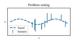
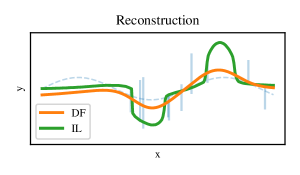
Figure 1: Interval regression. See Appendix D for the exact reproducible experimental setup (Left) Setup. The goal is to learn $f^{*}:\mathcal{X}\to\mathbb{R}$ represented by the dashed line, given samples $(x_{i},s_{i})$, where $(s_{i})$ are intervals represented by the blue segments. (Right) We compare the Infimum Loss (IL) baseline (13) shown in green, with our Disambiguation Framework (DF), Eqs. (4) and (5), shown in orange; with weights $\alpha$ given by kernel ridge regression. (DF) retrieves $\hat{y_{i}}$ before learning a smooth $f_{n}$ based on $(x_{i},\hat{y}_{i})$, while (IL) implicitly retrieves $\hat{y}_{i}(x)$ differently for each input, leading to irregularity of the consequent estimator of $f^{*}$.

Remark 7 (IQP implementation for Eq. (4)).

Other heuristics to solve Eq. (4) are conceivable. For example, considering $z_{i}=y_{i}$ in this equation, we remark that the resulting problem is isomorphic to an integer quadratic program (IQP). Similarly to integer linear programming, this problem can be approached with relaxation of the “integer constraint” to get a real-valued solution, before “thresholding” it to recover an integer solution. This heuristic can be seen as a generalization of the Diffrac algorithm (Bach & Harchaoui, 2007; Joulin et al., 2010). we present it in details in Appendix B.

Remark 8 (Link with EM, (Dempster et al., 1977)).

Arguably, our alternative minimization scheme, optimizing respectively the targets $\xi_{i}=\varphi(y_{i})$ and the function estimates $\zeta_{i}=\psi(f_{n}(x_{i}))$ can be seen as the non-parametric version of the Expectation-Maximization algorithm, popular for parametric model (Dempster et al., 1977).

5.4 Application: Ranking with partial ordering

Ranking is a problem consisting, for an input $x$ in an input space $\mathcal{X}$, to learn a total ordering $y$, belonging to $\mathcal{Y}=\mathfrak{S}_{m}$, modelling preference over $m$ items. It is usually approach with the Kendall loss $\ell(y,z)=-\varphi(y)^{\top}\varphi(z)$, with $\varphi(y)=(\operatorname{sign}\left(y(i)-y(j)\right))_{i,j\leq m}\in\left\{-1,1\right\}^{m^{2}}$ (Kendall, 1938). Full supervision corresponds, for a given $x$, to be given a total ordering of the $m$ items. This is usually not an option, but one could expect to be given partial ordering that $y$ should follow (Cao et al., 2007; Hüllermeier et al., 2008; Korba et al., 2018). Formally, this equates to the observation of some, but not all, coordinates $\varphi(y)_{i}$ of the vector $\varphi(y)$ for some $i\in I\subset\left\llbracket 1,m\right\rrbracket^{2}$.

In this setting, $s\subset\mathcal{Y}$ is a set of total orderings that match the given partial ordering. It can be represented by a vector $\xi_{s}\in{\cal H}$, that satisfies the partial ordering observation, $(\xi_{s})_{I}=\varphi(y)_{I}$, and that is agnostic on unobserved coordinates, $(\xi_{s})_{{}^{c}I}=0$. This vector satisfies that $z\to\psi(z)^{\top}\xi_{s}$ is minimized for, and only for, $z\in s$. Hence, it constitutes a good initialization for the alternative minimization scheme detailed above. We provide details in Appendix A.5, where we also show that $\xi_{s}$ can be formally translated in a $\mu_{s}$ to match the Definition 5, proving that ranking with partial labelling is a well-behaved problem.

Many real world problems can be formalized as a ranking problem with partial ordering observations. For example, $x$ could be a social network user, and the $m$ items could be posts of her connection that the network would like to order on her feed accordingly to her preferences. One might be told that the user $x$ prefer posts from her close rather than from her distant connections, which translates formally as the constraint that for any $i$ corresponding to a post of a close connection and $j$ corresponding to a post of a distant connection, we have $\varphi(y)_{ij}=1$. Nonetheless, designing non-parametric structured prediction models that scale well when the intrinsic dimension $m$ of the space $\mathcal{Y}$ is very large (such as the number of post on a social network) remains an open problem, that this paper does not tackle.

6 Related work

Weakly supervised learning has been approached through parametric and non-parametric methods. Parametric models are usually optimized through maximum likelihood (Heitjan & Rubin, 1991; Jin & Ghahramani, 2002). Hüllermeier (2014) show that this approach, as formalized by Denoeux (2013), equates to disambiguating sets by averaging candidates, which was shown inconsistent by Cabannes et al. (2020) when data are not missing at random. Among non-parametric models, Xu et al. (2004); Bach & Harchaoui (2007) developed an algorithm for clustering, that has been cast for weakly supervised learning problem (Joulin et al., 2010; Alayrac et al., 2016), leading to a disambiguation algorithm similar than ours, yet without consistency results. More recently, half-way between theory and practice, Gong et al. (2018) derived an algorithm geared towards classification, based on a disambiguation objective, incorporating several heuristics, such as class separation, and Laplacian diffusion. Those heuristics could be incorporated formally in our model.

The infimum loss principle has been considered by several authors, among them Cour et al. (2011); Luo & Orabona (2010); Hüllermeier (2014). It was recently analyzed through the prism of structured prediction by Cabannes et al. (2020), leading to a consistent non-parametric algorithm that will constitute the baseline of our experimental comparison. This principle is interesting as it does not assume knowledge on the corruption process $(S|Y)$ contrarily to the work of Cid-Sueiro et al. (2014) or van Rooyen & Williamson (2017).

The non-ambiguity assumption has been introduced by Cour et al. (2011) and is a classical assumption of learning with partial labelling (Liu & Dietterich, 2014). Assumptions of Lipschitzness and minimal mass are classical assumptions to prove convergence of local averaging method (Audibert & Tsybakov, 2007; Biau & Devroye, 2015). Those assumptions imply class separation in $\mathcal{X}$, which has been leverage in semi-supervised learning, justifying Laplacian regularization (Rigollet, 2007; Zhu et al., 2003).

Note that those assumptions might not hold on raw representation of the data, but with appropriate metrics, which could be learned through unsupervised (Duda et al., 2000) or self-supervised learning (Doersch & Zisserman, 2017). Indeed, Wei et al. (2021) provide an analysis akin ours based on such an assumption. As such, the practitioner might consider weights $\alpha$ given by similarity metrics derived through such techniques, before computing the disambiguation (4) and learning $f_{n}$ from the recollected fully supervised dataset with deep learning.

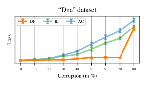
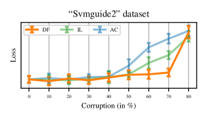
Figure 2: Testing errors as function of the supervision corruption on real dataset corresponding to classification with partial labels. We split fully supervised LIBSVM datasets into training and testing dataset. We corrupt training data in order to get partial labels. Corruption is managed through a parameter, represented by the $x$-axis, that relates to the ambiguity degree $\eta$ of Assumption 2. For each methods (our algorithm (DF), the baseline (IL), and the baseline of the baseline (AC, consisting of averaging candidates $y_{i}$ in sets $S_{i}$)), we consider weights $\alpha$ given by kernel ridge regression with Gaussian kernel, for which we optimized hyperparameters with cross-validation on the training set. We then learn an estimate $f_{n}$ that we evaluate on the testing set, represented by the $y$-axis, on which we have full supervision. The figure show the superiority of our method, that achieves error similar to baseline when full supervision ($x=0$) or no supervision ($x=100\%$) is given, but performs better when only in presence of partial supervision. See Appendix D for reproducibility specifications, where we also provide Figure 6 showcasing similar empirical results in the case of ranking with partial ordering.

7 Experiments

In this section, we review a baseline, and experiments that showcase the usefulness of our algorithm Eqs. (4) and (5).

Baseline.

We consider as a baseline the work of Cabannes et al. (2020), which is a consistent structured prediction approach to partial labelling through the infimum loss. It is arguably the state-of-the-art of partial labelling approached through structured prediction. It follow the same loss-based variance disambiguation principle, yet in an implicit fashion, leading to the inference algorithm, $f_{n}:\mathcal{X}\to\mathcal{Y}$,

$$f_{n}(x)\in\operatorname*{arg\,min}_{z\in\mathcal{Y}}\inf_{(y_{i})\in C_{n}}\sum_{i=1}^{n}\alpha_{i}(x)\ell(z,y_{i}).$$ (13)

Note that with our proof technique, which overcome the sub-optimality of calibration inequality (Audibert & Tsybakov, 2007; Cabannes et al., 2021), exponential convergence rates similar to Theorem 4 could be derived for the baseline. Yet, as we will see, our algorithm outperforms this state-of-the-art baseline. This could be explained by the fact that our algorithm introduce an intrinsically smaller surrogate space (in essence, Cabannes et al. (2020) introduced surrogate functions from inputs in $\mathcal{X}$ to powersets represented in $\mathbb{R}^{2^{\mathcal{Y}}}$, while we look at functions from input in $\mathcal{X}$ to output represented in $\mathbb{R}^{\mathcal{Y}}$).

Disambiguation coherence - Interval regression.

The baseline Eq. (13) implicitly requires to disambiguate $(\hat{y}_{i}(x))$ differently for every $x\in\mathcal{X}$. This is counter intuitive since $(y_{i}^{*})$ does not depend on $x$. It means that $(\hat{y}_{i})$ could be equal to some $(\hat{y}_{i}^{(0)})$ on a subset $\mathcal{X}_{0}$ of $\mathcal{X}$, and to another $(\hat{y}_{i}^{(1)})$ on a disjoint subset $\mathcal{X}_{1}\subset\mathcal{X}$, leading to irregularity of $f_{n}$ between $\mathcal{X}_{0}$ and $\mathcal{X}_{1}$. We illustrate this graphically on Figure 1. This figure showcases an interval regression problem, which corresponds to the regression setup ($\mathcal{Y}=\mathbb{R}$, $\ell(y,z)=\left|y-z\right|^{2}$) of partial labelling, where one does not observed $y\in\mathbb{R}$ but an interval $s\subset\mathbb{R}$ containing $y$. Among others, this problem appears in physics (Sheppard, 1897) and economy (Tobin, 1958).

Computation attractiveness - Ranking.

Computationally, the baseline requires to solve a disambiguation problem, recovering $(\hat{y_{i}}(x))\in C_{n}$ for every $x\in\mathcal{X}$ for which we want to infer $f_{n}(x)$. This is much more costly, than doing the disambiguation of $(\hat{y_{i}})\in C_{n}$ once, and solving the supervised learning inference problem Eq. (5), for every $x\in\mathcal{X}$ for which we want to infer $f_{n}(x)$. To illustrate the computation attractiveness of our algorithm, consider the case of ranking, defined in Section 5.4. Fully supervised inference scheme (5) corresponds to solving a NP-hard problem, equivalent to the minimum feedback arcset problem (Duchi et al., 2010). While disambiguation approaches with alternative minimization implied by Eq. (4) and Eq. (13) require to solve this NP-hard problem for each minimization step. In other terms, the baseline ask to solve multiple NP-hard problem every time one wants to infer $f_{n}$ given by Eq. (13) on an input $x\in\mathcal{X}$. Meanwhile, our disambiguation approach asks to solve multiple NP-hard problem upfront to solve Eq. (4), yet only require to solve one NP-hard problem to infer $f_{n}$ given by Eq. (5) on an input $x\in\mathcal{X}$.

Better empirical results - Classification.

Finally, we compare our algorithm, our baseline (13) and the baseline considered by Cabannes et al. (2020) on real datasets from the LIBSVM dataset (Chang & Lin, 2011). Those datasets $(x_{i},y_{i})$ correspond to fully supervised classification problem. In this setup, $\mathcal{Y}=\left\llbracket 1,m\right\rrbracket$ for $m$ a number of classes, and $\ell(y,z)=\mathbf{1}_{y\neq z}$. We “corrupt” labels in order to create a synthetic weak supervision datasets $(x_{i},s_{i})$. We consider skewed corruption, in the sense that $(s_{i})$ is generated by a probability such that $\sum_{z\in\mathcal{Y}}\operatorname{\mathbb{P}}_{S_{i}}(z\in S_{i}|y_{i})$ depends on the value of $y_{i}$. This corruption is parametrized by a parameter that related with the ambiguity parameter $\eta$ of Assumption 2. Results on Figure 2 show that, in addition to having a lower computation cost, our algorithm performs better in practice than the state-of-the-art baseline.

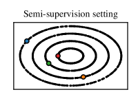
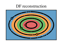
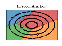
Figure 3: Semi-supervised learning, “concentric circle” instance with four classes (red, green, blue, yellow). Reproducibility details provided in Appendix D. (Left) We represent points $x_{i}\in\mathcal{X}\subset\mathbb{R}^{2}$, there is many unlabelled points (represented by black dots and corresponding to $S_{i}=\mathcal{Y}$), and one labelled point for each class (represented in color, corresponding to $S_{i}=\left\{y_{i}\right\}$). (Middle) Reconstruction $f_{n}:\mathcal{X}\to\mathcal{Y}$ given by our algorithm Eqs. (4) and (5). Our algorithm succeeds to comprehend the concentric circle structure of the input distribution and clusters classes accordingly. (Right) Reconstruction $f_{n}:\mathcal{X}\to\mathcal{Y}$ given by the baseline Eq. (13). The baseline performs as if only the four supervised data points where given.

Beyond Eq. (2) - Semi-supervised learning.

The main limitation of Eq. (2) is that it is a pointwise principle that decorrelates inputs, in the sense that the optimization of $\mu^{*}|_{x}$, for $x\in\mathcal{X}$, only depends on $\nu|_{x}$ and not on what is happening on $\mathcal{X}\backslash\left\{x\right\}$. As such, this principle failed to tackle semi-supervised learning, where $\nu|_{x}$ is equal to $\mu|_{x}$ (in the sense that $\pi|_{x,y}=\delta_{\left\{y\right\}}$) for $x\in\mathcal{X}_{l}$ and is equal to $\delta_{\mathcal{Y}}$ for $x\in\mathcal{X}_{u}:=\mathcal{X}\backslash\mathcal{X}_{l}$. In such a setting, for $x\in\mathcal{X}_{u}$, $\mu^{*}|_{x}$ can be set to any $\delta_{y}$ for $y\in\mathcal{Y}$. Interestingly, in practice, while the baseline suffer the same limitation, for our algorithm, weighting schemes have a regularization effect, that contrasts with those considerations. We illustrate it on Figure 3.

Real real-world applications.

There is a real lack of clean datasets to experiment with partial labelling. Most theoretical papers consist in synthetic corruption of fully supervised dataset (e.g., Korba et al., 2018) as we did. Empirical papers are built on highly complex datasets that require skilled pre-processing and tricks beside theoretically-grounded principle (e.g., action recognition on Youtube videos). However, note that the state-of-the-art work of Miech et al. (2019) is built on heuristics from the Diffrac algorithm, which we generalized (see Alayrac et al., 2016, for details). We hope that, by providing theoretical understanding of the problem, our paper could help to design powerful heuristics in practice, even though this is out of scope of the present paper.

8 Conclusion

In this work, we have introduced a structured prediction algorithm Eqs. (4) and (5), to tackle partial labelling. We have derived exponential convergence rates for the nearest neighbors instance of this algorithm under classical learnability assumptions. We provided optimization considerations to implement this algorithm in practice, and have successfully compared it with the state-of-the-art. Several open problems offer prospective follow-up of this works.

• Semi-supervised learning and beyond. While we only proved convergence in situation where $\mu^{*}$ of Eq. (2) is uniquely defined, therefore excluding semi-supervised learning, Figure 3 suggests that our algorithm (4) could be analyzed in a broader setting than the one considered in this paper. Among others, the non-ambiguity assumption could be replaced by a cluster assumption (Rigollet, 2007) together with a non-ambiguity assumption cluster-wise in Theorem 4.

• Hard-coded weak supervision. Variational principles Eqs. (2) and (3) could be extended beyond partial labelling to any type of hard-coded weak supervision, which is when weak supervision can be cast as a set of hard constraint that $\mu$ should satisfy, formally written as a set of fully supervised distributions compatible with weak information. Hard-coded weak supervision includes label proportion (Quadrianto et al., 2009; Dulac-Arnold et al., 2019), but excludes supervision of the type “80% of the experts say this nose is broken, and 20% say it is not”. Providing a unifying framework for those problems would make an important step in the theoretical foundation of weakly supervised learning.

• Missing input data. While weak supervision assumes that only $y$ is partially known, in many applications of machine learning, $x$ is also only partially known, especially when the feature vector $x$ is built from various source of information, leading to missing data. While we only considered a principle to fill missing output information, similar principles could be formalized to fill missing input information. This would be particularly valuable when data are not missing at random (Rubin, 1976; Muzellec et al., 2020).

Appendix A Proofs

Mathematical assumptions.

To make formal what should be seen as implicit assumptions heretofore, we consider $\mathcal{X}$ and $\mathcal{Y}$ Polish spaces, $\mathcal{Y}$ compact, $\ell:\mathcal{Y}\times\mathcal{Y}\to\mathbb{R}$ continuous, ${\cal H}$ a separable Hilbert space, $\varphi$ measurable, and $\psi$ continuous. We also assume that for $\nu_{x}$-almost every $x\in\mathcal{X}$, and any $\mu\vdash\nu$, that the pushforward measure $\varphi_{*}\mu|_{x}$ has a second moment. This is the sufficient setup in order to be able to define formally objects and solutions considered all along the paper.

Notations.

Beside standard notations, we use $\#\mathcal{Y}$ to design the cardinality of $\mathcal{Y}$, and $2^{\mathcal{Y}}$ to design the set of subsets of $\mathcal{Y}$. Regarding measures, we use $\mu_{\mathcal{X}}$ and $\mu|_{x}$ respectively the marginal over $\mathcal{X}$ and the conditional accordingly to $x$ of $\mu\in\Delta_{\mathcal{X}\times\mathcal{Y}}$. We denote by $\mu^{\otimes n}$ the distribution of the random variable $(Z_{1},\cdots,Z_{n})$, where the $Z_{i}$ are sampled independently according to $\mu$. For $A$ a Polish space, we consider $\Delta_{A}$ the set of Borel probability measures on this space. For $\varphi:\mathcal{Y}\to{\cal H}$ and $S\subset\mathcal{Y}$, we denote by $\varphi(S)$ the set $\left\{\varphi(y)\,\middle|\,y\in S\right\}$. For a family of sets $(S_{i})$, we denote by $\prod S_{i}$ the Cartesian product $S_{1}\times S_{2}\times\cdots$, also defined as the set of points $(y_{i})$ such that $y_{i}\in S_{i}$ for all index $i$, and by $\mathcal{Y}^{n}$ the Cartesian product $\prod_{i\leq n}\mathcal{Y}$. Finally, for $E$ a subset of a vector space $E^{\prime}$, $\operatorname{Conv}E$ denotes the convex hull of $E$ and $\operatorname{Span}(E)$ its span.

Abuse of notations.

For readability sake, we have abused notations. For a signed measure $\mu$, we denote by $\operatorname{\mathbb{E}}_{\mu}[X]$ the integral $\int x\mathop{}\!\mathrm{d}\mu(x)$, extending this notation usually reserved to probability measure. More importantly, when considering $2^{\mathcal{Y}}$, we should actually restrict ourselves to the subspace ${\cal S}\subset 2^{\mathcal{Y}}$ of closed subsets of $\mathcal{Y}$, as ${\cal S}$ is a Polish space (metrizable by the Hausdorff distance) while $2^{\mathcal{Y}}$ is not always. However, when $\mathcal{Y}$ is finite, those two spaces are equals, $2^{\mathcal{Y}}={\cal S}$.

A.1 Proof of Lemma 3

From Lemma 3 in Cabannes et al. (2021), we pulled the calibration inequality

$${\cal R}(f_{n})-{\cal R}(f^{*})\leq 2c_{\psi}\operatorname{\mathbb{E}}\left[\mathbf{1}_{\left\|g_{n}(X)-g^{*}(X)\right\|>d(g^{*}(X),F)}\left\|g_{n}(X)-g^{*}(X)\right\|\right].$$

Where $F$ is defined as the set of points $\xi\in\operatorname{Conv}\varphi(\mathcal{Y})$ leading to two decodings

$$F=\left\{\xi\in\operatorname{Conv}\varphi(\mathcal{Y})\,\middle|\,\#\operatorname*{arg\,min}_{z\in\mathcal{Y}}\left\langle\psi(z),\xi\right\rangle>1\right\},$$

and $d$ is defined as the extension of the norm distance to sets, for $\xi\in{\cal H}$

$$d(\xi,F)=\inf_{\xi^{\prime}\in F}\left\|\xi-\xi^{\prime}\right\|_{\cal H}.$$

Using that $\left\|g_{n}(X)-g^{*}(X)\right\|\leq\left\|g_{n}(X)-g_{n}^{*}(X)\right\|+\left\|g_{n}^{*}(X)-g^{*}(X)\right\|$ and that, if $a\leq b+c$,

$$\mathbf{1}_{a>\delta}a\leq\mathbf{1}_{b+c>\delta}b+c\leq\mathbf{1}_{2\sup(b,c)>\delta}2\sup{b,c}=2\sup_{e\in{b,c}}\mathbf{1}_{e>\delta}e\leq 2\mathbf{1}_{b>\delta}b+2\mathbf{1}_{c>\delta}c.$$

We get the refined inequality

$${\cal R}(f_{n})-{\cal R}(g^{*})\leq 4c_{\psi}\operatorname{\mathbb{E}}\left[\mathbf{1}_{2\left\|g_{n}(X)-g_{n}^{*}(X)\right\|>d(g^{*}(X),F)}\left\|g_{n}(X)-g_{n}^{*}(X)\right\|+\mathbf{1}_{2\left\|g_{n}^{*}(X)-g^{*}(X)\right\|>d(g^{*}(X),F)}\left\|g_{n}^{*}(X)-g^{*}(X)\right\|\right].$$

The first term is bounded with

$$\operatorname{\mathbb{E}}\left[\mathbf{1}_{2\left\|g_{n}(X)-g_{n}^{*}(X)\right\|>d(g^{*}(X),F)}\left\|g_{n}(X)-g_{n}^{*}(X)\right\|\right]\leq\left\|g_{n}-g_{n}^{*}\right\|_{L^{1}}.$$

While for the second term, we proceed with

$$\operatorname{\mathbb{E}}\left[\mathbf{1}_{2\left\|g_{n}^{*}(X)-g^{*}(X)\right\|>d(g^{*}(X),F)}\left\|g_{n}^{*}(X)-g^{*}(X)\right\|\right]\leq\left\|g_{n}^{*}-g^{*}\right\|_{L^{\infty}}\operatorname{\mathbb{P}}_{X}\left(2\left\|g_{n}^{*}(X)-g^{*}(X)\right\|>\inf_{x\in\operatorname*{supp}\nu_{\mathcal{X}}}d(g^{*}(X),F)\right).$$

When weights sum to one, that is $\sum_{i=1}^{n}\alpha_{i}(X)=1$, both $g_{n}^{*}(X)$ and $g^{*}(X)$ are averaging of $\varphi(y)$ for $y\in\mathcal{Y}$, therefore

$$\left\|g_{n}^{*}-g^{*}\right\|_{L^{\infty}}\leq 2c_{\varphi}.$$

Finally, when the labels are a deterministic function of the input, $g^{*}(X)=\varphi(f^{*}(X))$, and $d(g^{*}(X),F)\leq\sup_{y\in\mathcal{Y}}d(\varphi(y),F)$. Defining $\delta:=\sup_{y\in\mathcal{Y}}d(\varphi(y),F)/2$, and adding everything together leads to Lemma 3.

A.2 Implication of Assumptions 2 and 3

Assume that Assumption 2 holds, consider $x\in\operatorname*{supp}\nu_{\mathcal{X}}$, let us show that $f^{*}(x)=y_{x}$ and $\mu^{*}|_{x}=\delta_{y_{x}}$. First of all, notice that $\bigcap_{S;S\in\operatorname*{supp}\nu|_{x}}=\left\{y_{x}\right\}$; that $\delta_{y_{x}}\vdash\nu|_{x}$, as it corresponds to $\pi|_{x,S}=\delta_{y_{x}}\in\Delta_{S}$, for all $S$ in the support of $\nu|_{x}$; and that, because $\ell$ is well-behaved,

$$\inf_{z\in\mathcal{Y}}\ell(z,y_{x})=\ell(y_{x},y_{x})=0.$$

This infimum is only achieved for $z=y_{x}$, hence if we prove that $\mu^{*}|_{x}=\delta_{y_{x}}$, we directly have that $f^{*}(x)=y_{x}$. Finally, suppose that $\mu|_{x}\vdash\nu|_{x}$ charges $y\neq y_{x}$. Because $y$ does not belong to all sets charged by $\nu|_{x}$, $\mu|_{x}$ should charge an other $y^{\prime}\in\mathcal{Y}$, and therefore

$$\inf_{z\in\mathcal{Y}}\operatorname{\mathbb{E}}_{Y\sim\mu|_{x}}[\ell(z,y)]\geq\inf_{z\in\mathcal{Y}}\mu|_{x}(y)\ell(z,y)+\mu|_{x}(y^{\prime})\ell(z,y^{\prime})>0.$$

Which shows that $\mu^{*}|_{x}=\delta_{y_{x}}$. We deduce that $g^{*}(x)=y_{x}$.

Now suppose that Assumption 3 holds too, and consider two $x,x^{\prime}\in\operatorname*{supp}\nu_{\mathcal{X}}$ belonging to two different classes $f(x)=y$ and $f(x^{\prime})=y^{\prime}$. We have that $g^{*}(x)=\varphi(y)$ and $g^{*}(x^{\prime})=\varphi(y^{\prime})$, therefore,

$$d(x,x^{\prime})\geq c^{-1}\left\|\varphi(y)-\varphi(y^{\prime})\right\|_{\cal H}.$$

Define $h_{2}=\inf_{y\neq y^{\prime}}c^{-1}\left\|\varphi(y)-\varphi(y^{\prime})\right\|_{\cal H}$. Let us now show that $h_{2}>0$. When $\mathcal{Y}$ is finite, this infimum is a minimum, therefore, $h_{2}=0$, only if there exists a $y\neq y^{\prime}$, such that $\varphi(y)=\varphi(y^{\prime})$, which would implies that $\ell(\cdot,y)=\ell(\cdot,y^{\prime})$ and therefore $\ell(y,y^{\prime})=\ell(y,y)$ which is impossible when $\ell$ is proper.

A.3 Proof of Theorem 4

Reusing Lemma 3, we have

$${\cal E}(f_{n})\leq 4c_{\psi}\operatorname{\mathbb{E}}_{{\cal D}_{n},X}\left[\left\|g_{n}^{*}(X)-g_{n}(X)\right\|_{\cal H}\right]+8c_{\psi}c_{\varphi}\operatorname{\mathbb{E}}_{{\cal D}_{n},X}\left[\mathbf{1}_{\left\|g_{n}^{*}(X)-g^{*}(X)\right\|>\delta}\right].$$

We will first prove that

$$\operatorname{\mathbb{E}}_{{\cal D}_{n}}\left[\mathbf{1}_{\left\|g_{n}^{*}(X)-g^{*}(X)\right\|>\delta}\right]\leq\exp\left(-\frac{np}{8}\right)$$

as long as $k<np/2$. The error between $g^{*}$ and $g_{n}$ relates to classical supervised learning of $g^{*}$ from samples $(X_{i},Y_{i})\sim\mu^{*}$. We invite the reader who would like more insights on this fully supervised part of the proof to refer to the several monographs written on local averaging methods and, in particular, nearest neighbors, such as Biau & Devroye (2015). Because of class separation, we know that, if $k$ points fall at distance at most $h$ of $x\in\operatorname*{supp}\nu_{\mathcal{X}}$, $g_{n}^{*}(x)=k^{-1}\sum_{i;X_{i}\in{\cal N}(x)}\varphi(y_{i})=\varphi(y_{x})=g^{*}(x)$, where ${\cal N}(x)$ designs the $k$-nearest neighbors of $x$ in $(X_{i})$. Because the probability of falling at distance $h$ of $x$ for each $X_{i}$ is lower bounded by $p$, we have that

$$\operatorname{\mathbb{P}}_{{\cal D}_{n}}(g_{n}^{*}(x)\neq g^{*}(x))\leq\operatorname{\mathbb{P}}(\text{Bernouilli}(n,p)<k).$$

This can be upper bound by $\exp(-np/8)$ as soon as $k<np/2$, based on Chernoff multiplicative bound (see Biau & Devroye, 2015, for a reference), meaning

$$\operatorname{\mathbb{E}}_{{\cal D}_{n},X}\left[\mathbf{1}_{\left\|g_{n}^{*}(X)-g^{*}(X)\right\|\geq\delta}\right]\leq\exp(-np/8).$$

For the disambiguation part in $\left\|g_{n}-g_{n}^{*}\right\|_{L^{1}}$, we distinguish two types of datasets, the ones where for any input $X_{i}$ its $k$-neighbors at are distance at least $h$, ensuring that disambiguation can be done by clusters, and datasets that does not verify this property. Consider the event

$$\mathbb{D}=\left\{(X_{i})_{i\leq n}\,\middle|\,\sup_{i}d(X_{i},X_{(k)}(X_{i}))<h\right\}$$

where $X_{(k)}(x)$ design the $k$-th nearest neighbor of $x$ in $(X_{i})_{i\leq n}$. We proceed with

$$\operatorname{\mathbb{E}}_{{\cal D}_{n},X}\left[\left\|g_{n}^{*}(X)-g_{n}(X)\right\|_{\cal H}\right]\leq\sup_{X\in\mathcal{X}}\left\|g_{n}^{*}-g_{n}\right\|_{\infty}\operatorname{\mathbb{P}}_{{\cal D}_{n}}((X_{i})\notin\mathbb{D})+\operatorname{\mathbb{E}}_{{\cal D}_{n},X}\left[\left\|g_{n}^{*}(X)-g_{n}(X)\right\|_{\cal H}\,\middle|\,(X_{i})\in\mathbb{D}\right],$$

Which is based on $E[Z]=\operatorname{\mathbb{P}}(Z\in A)\operatorname{\mathbb{E}}[Z|A]+\operatorname{\mathbb{P}}(Z\notin A)\operatorname{\mathbb{E}}[Z|^{c}A]$. For the term corresponding to bad datasets, we can bound the disambiguation error with the maximum error. Similarly to the derivation for Lemma 3, because $g_{n}^{*}(x)$ and $g_{n}^{*}(X)$, are averaging of $\varphi(y)$, we have that

$$\sup_{x\in\operatorname*{supp}\nu_{\mathcal{X}}}\left\|g_{n}(x)-g_{n}^{*}(x)\right\|\leq 2c_{\varphi}.$$

Indeed, we allow ourselves to pay the worst error on those datasets as their probability is really small, which can be proved based on the following derivation.

$$\operatorname{\mathbb{P}}_{{\cal D}_{n}}((X_{i})_{i\leq n}\notin\mathbb{D}) =\operatorname{\mathbb{P}}_{(X_{i})}(\sup_{i}d(X_{i},X_{(k)}(X_{i}))\geq h)=\operatorname{\mathbb{P}}_{(X_{i})}\left(\cup_{i\leq n}\left\{d(X_{i},X_{(k)}(X_{i}))\geq h\right\}\right)$$

$$\leq\sum_{i=1}^{n}\operatorname{\mathbb{P}}_{(X_{i})}\left(d(X_{i},X_{(k)}(X_{i}))\geq h\right)=n\operatorname{\mathbb{P}}_{X,{\cal D}_{n-1}}\left(d(X,X_{(k)}(X))\geq h\right).$$

This last probability has already been work out when dealing with the fully supervised part, and was bounded as

$$\operatorname{\mathbb{P}}_{X,{\cal D}_{n-1}}\left(d(X,X_{(k)}(X))\geq h\right)\leq\exp\left(-(n-1)p/8\right).$$

as long as $k<(n-1)p/2$. Finally we have

$$\sup_{X\in\mathcal{X}}\left\|g_{n}^{*}-g_{n}\right\|_{\infty}\operatorname{\mathbb{P}}_{{\cal D}_{n}}((X_{i})_{i\leq n}\notin\mathbb{D})\leq 2c_{\varphi}n\exp\left(-(n-1)p/8\right).$$

For the expectation term, corresponding to datasets, ${\cal D}_{n}\in\mathbb{D}$, that cluster data accordingly to classes, we have to make sure that $\hat{y}_{i}=y_{i}^{*}$ is the only acceptable solution of Eq. (4), which is true as soon as the intersection of $S_{j}$, for $x_{j}$ the neighbors of $x_{i}$, only contained $y_{i}^{*}$. To work out the disambiguation algorithm, notice that

$$\left\|g_{n}-g_{n}^{*}\right\|_{L^{1}} =\int_{\mathcal{X}}\left\|\sum_{i=1}^{n}\alpha_{i}(x)\varphi(\hat{y}_{i})-\varphi(y^{*}_{i})\right\|\mathop{}\!\mathrm{d}\nu_{\mathcal{X}}(x)\leq\int_{\mathcal{X}}k^{-1}\sum_{i=1}^{n}\mathbf{1}_{X_{i}\in{\cal N}(x)}\left\|\varphi(\hat{y}_{i})-\varphi(y^{*}_{i})\right\|\mathop{}\!\mathrm{d}\nu_{\mathcal{X}}(x)$$

$$=k^{-1}\sum_{i=1}^{n}\operatorname{\mathbb{P}}_{X}\left(X_{i}\in{\cal N}(X)\right)\left\|\varphi(\hat{y}_{i})-\varphi(y^{*}_{i})\right\|\leq 2c_{\varphi}k^{-1}\sum_{i=1}^{n}\operatorname{\mathbb{P}}_{X}\left(X_{i}\in{\cal N}(X)\right)\mathbf{1}_{\varphi(\hat{y}_{i})\neq\varphi(y^{*}_{i})}.$$

Finally we have, after proper conditionning, considering the variability in $S_{i}$ while fixing $X_{i}$ first,

$$\operatorname{\mathbb{E}}_{{\cal D}_{n},X}\left[\left\|g_{n}^{*}(X)-g_{n}(X)\right\|_{\cal H}\,\middle|\,(X_{i})\in\mathbb{D}\right] =2c_{\varphi}k^{-1}\operatorname{\mathbb{E}}_{(X_{i})}\left[\sum_{i=1}^{n}\operatorname{\mathbb{P}}_{X}\left(X_{i}\in{\cal N}(X)\right)\operatorname{\mathbb{E}}_{(S_{i})}\left[\mathbf{1}_{\varphi(\hat{y}_{i})\neq\varphi(y^{*}_{i})}\,\middle|\,(X_{i})\right]\,\middle|\,(X_{i})\in\mathbb{D}\right]$$

$$=2c_{\varphi}k^{-1}\operatorname{\mathbb{E}}_{(X_{i}),X}\left[\sum_{i=1}^{n}\mathbf{1}_{X_{i}\in{\cal N}(X)}\operatorname{\mathbb{P}}_{(S_{i})}\left(\varphi(\hat{y}_{i})\neq\varphi(y^{*}_{i})\,\middle|\,(X_{i})\right)\,\middle|\,(X_{i})\in\mathbb{D}\right].$$

We design $\mathbb{D}$, because when this event holds, we know that the $k$-th nearest neighbor of any input $X_{i}$ is at distance at most $h$ of $X_{i}$, meaning the because of class separation, $y_{x_{i}}\in S_{j}$ for any $X_{j}\in{\cal N}(X_{i})$. This mean that outputting $(\hat{y}_{i})=(y^{*}_{i})$ and $z_{j}=y_{j}$, will lead to an optimal error in Eq. (4). Now suppose that there is an other solution for Eq. (4) such that $\hat{y}_{i}\neq y_{i}^{*}$, it should also achieve an optimal error, therefore it should verify $z_{j}=\hat{y}_{j}$ for all $j$ as well as $\hat{y}_{j}=\hat{y}_{i}$ for all $j$ such that $X_{j}$ is one of the $k$ nearest neighbors of $X_{i}$. This implies that $\hat{y}_{i}\in\cap_{j;X_{j}\in{\cal N}(X_{i})}S_{j}$, which happen with probability

$$\operatorname{\mathbb{P}}_{(S_{j})_{j;X_{j}\in{\cal N}(X_{i})}}(\exists z\neq y_{i},z\in\cap_{j}S_{j})\leq m\operatorname{\mathbb{P}}_{S_{j}}(z\in S_{j})^{k}\leq m\eta^{k}=m\exp(-k\left|\log(\eta)\right|).$$

With $m=\#\mathcal{Y}$ the number of element in $\mathcal{Y}$. We deduce that

$$\operatorname{\mathbb{P}}_{(S_{i})}\left(\varphi(\hat{y}_{i})\neq\varphi(y^{*}_{i})\,\middle|\,(X_{i})\right)\leq m\exp(-k\left|\log(\eta)\right|).$$

And because $\sum_{i=1}^{n}\mathbf{1}_{X_{i}\in{\cal N}(X)}=k$, we conclude that

$$\operatorname{\mathbb{E}}_{{\cal D}_{n},X}\left[\left\|g_{n}^{*}(X)-g_{n}(X)\right\|_{\cal H}\,\middle|\,(X_{i})\in\mathbb{D}\right]\leq 2c_{\varphi}m\exp(-k\left|\log(\eta)\right|).$$

Finally, adding everything together we get

$${\cal E}(f_{n})\leq 8c_{\varphi}c_{\psi}\exp\left(-\frac{np}{8}\right)+8c_{\varphi}c_{\psi}n\exp\left(-\frac{(n-1)p}{8}\right)+8c_{\varphi}c_{\psi}m\exp\left(-k\left|\log(\eta)\right|\right).$$

as long as $k<(n-1)p/2$, which implies Theorem 4 as long as $n\geq 2$.

Remark 9 (Other approaches).

While we have proceed with analysis based on local averaging methods, other paths could be explored to prove convergence results of the algorithm provided Eq. (4) and (5). For example, one could prove Wasserstein convergence of $\sum_{i=1}^{n}\delta_{(x_{i},\hat{y}_{i})}$ towards $\sum_{i=1}^{n}\delta_{(x_{i},\hat{y}^{*}_{i})}$, together with some continuity of the learning algorithm as a function of those distributions. This analysis could be understood as tripartite:

• A disambiguation error, comparing $\hat{y}_{i}$ to $y_{i}^{*}$.

• A stability / robustness measure of the algorithm to learn $f_{n}$ from data when substituting $y_{i}^{*}$ by $\hat{y}_{i}$.

• A consistency result regarding $f_{n}^{*}$ learnt on $(x_{i},y_{i}^{*})$.

Our analysis followed a similar path, yet with the first two parts tackled jointly.

A.4 Proof of Proposition 6

Under the non-ambiguity hypothesis (Assumption 2), the solution of Eq. (3) is characterized pointwise by $f^{*}(x)=y_{x}$ for all $x\in\operatorname*{supp}\nu_{\mathcal{X}}$. Similarly under Assumption 2, we have the characterization $f^{*}(x)\in\cap_{S\in\operatorname*{supp}\nu|_{x}}S$. With the notation of Definition 5, since $f^{*}(x)$ minimizes $z\to\operatorname{\mathbb{E}}_{Y\sim\mu_{S}}[\ell(z,Y)]$ for all $S\in\operatorname*{supp}\nu|_{x}$, it also minimizes $z\to\operatorname{\mathbb{E}}_{S\sim\nu|_{x}}\operatorname{\mathbb{E}}_{Y\sim\mu_{S}}[\ell(z,Y)]$.

For the second part of the proposition, we use the structured prediction framework of Ciliberto et al. (2020). Define the signed measure $\mu^{\circ}$ defined as $\mu^{\circ}_{\mathcal{X}}:=\nu_{\mathcal{X}}$ and $\mu^{\circ}|_{x}:=\operatorname{\mathbb{E}}_{S\sim\nu|_{x}}\operatorname{\mathbb{E}}_{Y\sim\mu_{S}}[\delta_{Y}]$, and $f^{\circ}:\mathcal{X}\to\mathcal{Y}$ the solution $f^{\circ}\in\operatorname*{arg\,min}_{f:\mathcal{X}\to\mathcal{Y}}\operatorname{\mathbb{E}}_{(X,Y)\sim\mu^{\circ}}[\ell(f(X),Y)]=\operatorname*{arg\,min}_{f:\mathcal{X}\to\mathcal{Y}}\operatorname{\mathbb{E}}_{(X,Y)\sim\nu}\left[\operatorname{\mathbb{E}}_{Y\sim\mu_{S}}[\ell(f(X),Y)]\right]$. The first part of the proposition tells us that $f^{\circ}=f^{*}$ under Assumption 2. The framework of Ciliberto et al. (2020), tells us that $f^{\circ}$ is obtained after decoding, Eq. (9), of $g^{\circ}:\mathcal{X}\to{\cal H}$, and that if $g_{n}^{\circ}$ converges to $g^{\circ}$ with the $L^{1}$ norm, $f_{n}^{\circ}$ converges to $f^{\circ}$ in term of the $\mu^{\circ}$-risk. Under Assumption 2 and mild hypothesis on $\mu^{\circ}$, it is possible to prove that convergence in term of the $\mu^{\circ}$-risk implies convergence in term of the $\mu$-risk (for example through calibration inequality similar to Proposition 2 of Cabannes et al. (2020)).

A.5 Ranking with Partial ordering is a well behaved problem

Here, we discuss about building directly $\xi_{S}$ to initialize our alternative minimization scheme or considering $\mu_{S}$ given by the definition of well-behaved problem (Definition 5). Since the existence of $\mu_{S}$ implying $\xi_{S}$ defined as $\operatorname{\mathbb{E}}_{Y\sim\mu_{S}}[\varphi(Y)]$, we will only study when $\xi_{S}$ can be cast as a $\mu_{S}$.

In ranking, we have that $\psi=-\varphi$, which corresponds to “correlation losses”. In this setting, we have that $\operatorname{Span}(\varphi(\mathcal{Y}))=\operatorname{Span}(\psi(\mathcal{Y}))$. More generally, looking at a “minimal” representation of $\ell$, one can always assume the equality of those spans, as what happens on the orthogonal of the intersection of those spans, does not modify the scalar product $\varphi(y)^{\top}\psi(z)$. Similarly, $\xi_{S}$ can be restricted to $\operatorname{Span}(\psi(\mathcal{Y}))$, and therefore $\operatorname{Span}(\varphi(\mathcal{Y}))$, which exactly the image by $\mu\to\operatorname{\mathbb{E}}_{Y\sim\mu}[\varphi(Y)]$ of the set of signed measures, showing the existence of a $\mu_{S}$ matching Definition 5.

Appendix B IQP implementation for Eq. (4)

In this section, we introduce an IQP implementation to solve for Eq. (4). We first mention that our alternative minimization scheme is not restricted to well-behaved problem, before motivating the introduction of the IQP algorithm in two different ways, and finally describing its implementation.

B.1 Initialization of alternative minimization for non well-behaved problem

Before describing the IQP implementation to solve Eq. (12), we would like to stress that, even for non well-behaved partial labelling problems, it is possible to search for smart ways to initialize variables of the alternative minimization scheme. For example, one could look at $z_{i}^{(0)}\in\cap_{j;x_{j}\in{\cal N}_{k_{i}}}S_{j}$, where ${\cal N}_{k}$ designs the $k$ nearest neighbors of $x_{i}$ in $(x_{j})_{j\leq n}$, and $k_{i}$ is chosen such that this intersection is a singleton.

B.2 Link with Diffrac and empirical risk minimization

Our IQP algorithm is similar to an existing disambiguation algorithm known as the Diffrac algorithm (Bach & Harchaoui, 2007; Joulin et al., 2010). This algorithm was derived by implicitly following empirical risk minimization of Eq. (2). This approach leads to algorithms written as

$$(y_{i})\in\operatorname*{arg\,min}_{(y_{i})\in C_{n}}\inf_{f\in{\cal F}}\sum_{i=1}^{n}\ell(f(x_{i}),y_{i})+\lambda\Omega(f),$$

for ${\cal F}$ a space of functions, and $\Omega:{\cal F}\to\mathbb{R}_{+}$ a measure of complexity. Under some conditions, it is possible to simplify the dependency in $f$ (e.g., Xu et al., 2004; Bach & Harchaoui, 2007). For example, if $\ell(y,z)$ can be written as $\left\|\varphi(y)-\varphi(z)\right\|^{2}$ for a mapping $\varphi:\mathcal{X}\to\mathcal{Y}$, e.g. the Kendall loss detailed in Section 5.4, and the search of $\varphi(f):\mathcal{X}\to\varphi(\mathcal{Y})$ is relaxed as a $g:\mathcal{X}\to{\cal H}$. With $\Omega$ and ${\cal F}$ linked with kernel regression on the surrogate functional space $\mathcal{X}\to{\cal H}$, it is possible to solve the minimization with respect to $g$ as $g(x_{i})=\sum_{j=1}^{n}\alpha_{j}(x_{i})\varphi(y_{i})$, with $\alpha$ given by kernel ridge regression (Ciliberto et al., 2016), and to obtain a disambiguation algorithm written as

$$\operatorname*{arg\,min}_{y_{i}\in S_{i}}\sum_{i=1}^{n}\big{\|}\sum_{j=1}^{n}\alpha_{j}(x_{i})\varphi(y_{j})-\varphi(y_{i})\big{\|}^{2}.$$

This IQP is a special case of the one we will detail. As such, our IQP is a generalization of the Diffrac algorithm, and this paper provides, to our knowledge, the first consistency result for Diffrac.

B.3 Link with an other determinism measure

While we have considered the measure of determinism given by Eq. (2), we could have considered its quadratic variant

$$\mu^{\star}\in\operatorname*{arg\,min}_{\mu\vdash\nu}\inf_{f:\mathcal{X}\to\mathcal{Y}}\operatorname{\mathbb{E}}_{X\sim\nu_{\mathcal{X}}}\left[\operatorname{\mathbb{E}}_{Y,Y^{\prime}\sim\mu|_{x}}\left[\ell(Y,Y^{\prime})\right]\right].$$

This correspond to the right drawing of Figure 4. We could arguably translate it experimentally as

$$(\hat{y}_{i})\in\operatorname*{arg\,min}_{(y_{i})\in C_{n}}\sum_{i,j=1}^{n}\alpha_{i}(x_{j})\ell(y_{i},y_{j}),$$ (14)

and still derive Theorem 4 when substituting Eq. (4) by Eq. (14). When the loss is a correlation loss $\ell(y,z)=-\varphi(y)^{\top}\varphi(z)$. This leads to the quadratic problem

$$(\hat{y}_{i})\in\operatorname*{arg\,min}_{(y_{i})\in C_{n}}-\sum_{i,j=1}^{n}\alpha_{i}(x_{j})\varphi(y_{i})^{\top}\varphi(y_{j}).$$

B.4 IQP Implementation

In order to make our implementation possible for any symmetric loss $\ell:\mathcal{Y}\times\mathcal{Y}\to\mathbb{R}$, on a finite space $\mathcal{Y}$, we introduce the following decomposition.

Proposition 10 (Quadratic decomposition).

When $\mathcal{Y}$ is finite, any proper symmetric loss $\ell$ admits a decomposition with two mappings $\varphi:\mathcal{Y}\to\mathbb{R}^{m}$, $\psi:\mathcal{Y}\to\mathbb{R}^{m}$, for a $m\in\mathbb{N}$ and a $c\in\mathbb{R}$, reading

$$\forall\,y,z\in\mathcal{Y},\quad\ell(y,z)=\psi(y)^{\top}\psi(z)-\varphi(y)^{\top}\varphi(z)\qquad\text{with}\qquad\left\|\varphi(y)\right\|=\left\|\psi(y)\right\|=c$$ (15)

Proof.

Consider $\mathcal{Y}={y_{1},\cdot,y_{m}}$ and $L=(\ell(y_{i},y_{j}))_{i,j\leq m}\in\mathbb{R}^{m\times m}$. $L$ is a symmetric matrix, diagonalizable as $L=\sum_{i=1}^{m}\lambda_{i}u_{i}\otimes u_{i},$ with $(u_{i})$ a orthonormal basis of $\mathbb{R}^{m}$, and $\lambda_{i}\in\mathbb{R}$ its eigen values. We have, with $(e_{i})$ the Cartesian basis of $\mathbb{R}^{m}$,

$$\ell(y_{j},y_{k})=L_{jk}=\left\langle e_{j},Le_{k}\right\rangle=\sum_{i=1}^{m}(\lambda_{i})_{+}\left\langle e_{j},u_{i}\right\rangle\left\langle e_{k},u_{i}\right\rangle-\sum_{i=1}^{m}(\lambda_{i})_{-}\left\langle e_{j},u_{i}\right\rangle\left\langle e_{k},u_{i}\right\rangle.$$

We build the decomposition

$$\tilde{\psi}(y_{k})=\left(\sqrt{(\lambda_{i})_{+}}\left\langle e_{k},u_{i}\right\rangle\right)_{i\leq m},\qquad\text{and}\qquad\tilde{\varphi}(y_{k})=\left(\sqrt{(\lambda_{i})_{-}}\left\langle e_{k},u_{i}\right\rangle\right)_{i\leq m}.$$

It satisfies $\ell(y_{j},y_{k})=\tilde{\psi}(y)^{\top}\tilde{\psi}(z)-\tilde{\varphi}(y)^{\top}\tilde{\varphi}(z).$ We only need to show that we can consider $\varphi$ of constant norm. For this, first consider $C=\max_{i}\left|\lambda_{i}\right|$, we have $\left\|\tilde{\psi}(y_{k})\right\|^{2}=\sum_{i=1}^{m}(\lambda_{i})_{+}\left\langle u_{i},e_{k}\right\rangle^{2}\leq C\sum_{i=1}^{m}\left\langle u_{i},e_{k}\right\rangle^{2}=C\left\|e_{k}\right\|^{2}=C$ The last equalities being due to the fact that $(u_{i})$ is orthonormal. Now, introduce the correction vector $\xi:\mathcal{Y}\to\mathbb{R}^{m}$, $\xi(y_{i})=\sqrt{C-\left\|\tilde{\psi}(y)\right\|^{2}}e_{i}.$ And consider $\varphi=\binom{\tilde{\varphi}}{\xi}$, $\psi=\binom{\tilde{\psi}}{\xi}$. By construction, $\psi$ is of constant norm being equal to $C$ and that $\ell(y,z)=\psi(y)^{T}\psi(z)-\varphi(y)^{T}\varphi(z)$. Finally, because $\ell(y,z)=0$, we also have $\varphi$ of constant norm. ∎

Using the decomposition Eq. (15), Eq. (14) reads, with $\textbf{y}=(y_{i})$

$${\bf\hat{y}}\in\operatorname*{arg\,min}_{{\bf y}\in C_{n}}\sum_{i=1}^{n}\alpha_{i}(x_{j})\psi(y_{i})\psi(y_{j})-\sum_{i=1}^{n}\alpha_{i}(x_{j})\varphi(y_{i})\varphi(y_{j}).$$

By defining the matrix $A=(\alpha_{i}(x_{j}))_{ij\leq n}\in\mathbb{R}^{n\times n}$, $\Psi({\bf y})=(\psi(y_{i}))_{i\leq n}\in\mathbb{R}^{n\times m}$ and $\Phi({\bf y})=(\varphi(y_{i}))_{i\leq n}\in\mathbb{R}^{n\times m}$, we cast it as

$${\bf\hat{y}}\in\operatorname*{arg\,min}_{{\bf y}\in C_{n}}\operatorname{Tr}\left(A\Psi({\bf y})\Psi({\bf y})^{\top}\right)-\operatorname{Tr}\left(A\Phi({\bf y})\Phi({\bf y})^{\top}\right).$$

Objective convexification.

As $\alpha_{i}(x_{j})$ is a measure of similarity between $x_{i}$ and $x_{j}$, $A$ is usually symmetric positive definite, making this objective convex in $\Psi$ and concave in $\Phi$. However, recalling Eq. (15), we have $\operatorname{Tr}\Phi\Phi^{\top}=\operatorname{Tr}{\Psi\Psi^{\top}}=nc$, therefore considering the spectral norm of $A$, we convexify the objective as

$${\bf\hat{y}}\in\operatorname*{arg\,min}_{{\bf y}\in C_{n}}\operatorname{Tr}\left((\left\|A\right\|_{*}I+A)\Psi({\bf y})\Psi({\bf y})^{\top}\right)+\operatorname{Tr}\left((\left\|A\right\|_{*}I-A)\Phi({\bf y})\Phi({\bf y})^{\top}\right).$$

Considering

$$B=\left(\begin{array}[]{cc}\left\|A\right\|_{*}I+A&0\\ 0&\left\|A\right\|_{*}I-A\end{array}\right)\qquad\text{and}\quad\Xi({\bf y})=\binom{\Psi({\bf y})}{\Phi({\bf y})},$$

allow to simplify this objective as

$${\bf\hat{y}}\in\operatorname*{arg\,min}_{{\bf y}\in C_{n}}\operatorname{Tr}\left(B\Xi({\bf y})\Xi({\bf y})^{\top}\right).$$

When parametrized by $\xi=\Xi({\bf y})$, this is an optimization problem with a convex quadratic objective and “integer-like” constraint $\xi\in\Xi(C_{n})$, identifying to an integer quadratic program (IQP).

Relaxation.

IQP are known to be NP-hard, several tools exists in literature and optimization library implementing them. The most classical approach consists in relaxing the integer constraint $\xi\in\Xi(C_{n})$ into the convex constraint $\xi\in\operatorname{Conv}(\Xi(C_{n}))$, solving the resulting convex quadratic program, and projecting back the solution towards an extreme of the convex set. Arguably, our alternative minimization approach is a better grounded heuristic to solve our specific disambiguation problem.

Appendix C Example with graphical illustrations

Figure 4: Exposition of a pointwise problem in the simplex $\Delta_{\mathcal{Y}}$, with $\mathcal{Y}=\left\{a,b,c\right\}$ and a proper symmetric loss defined by $\ell(a,b)=\ell(a,c)=\ell(b,c)/2$. (Left) Representation of the decision regions $R_{z}=\left\{\mu\in\Delta_{\mathcal{Y}}\,\middle|\,z\in\operatorname*{arg\,min}_{z^{\prime}\in\mathcal{Y}}\operatorname{\mathbb{E}}_{Y\sim\mu}[\ell(z,y)]\right\}.$ for $z\in\mathcal{Y}$. (Middle Left) Representation of $R_{\nu}=\left\{\mu\in\Delta_{\mathcal{Y}}\,\middle|\,\mu\vdash\nu\right\}$ for $\nu=(5\delta_{\left\{a,b,c\right\}}+\delta_{\left\{c\right\}}+\delta_{\left\{a,c\right\}}+\delta_{\left\{b,c\right\}})/8$ (Middle Right) Level curves of the piecewise function $\Delta_{\mathcal{Y}}\to\mathbb{R};\mu\to\min_{z\in\mathcal{Y}}\operatorname{\mathbb{E}}_{Y\sim\mu}[\ell(z,Y)]$ corresponding to Eq. (2). (Right) Level curves of the quadratic function $\Delta_{\mathcal{Y}}\to\mathbb{R};\mu\to\operatorname{\mathbb{E}}_{Y,Y^{\prime}\sim\mu}[\ell(Y,Y^{\prime})]$. Our disambiguation (2) corresponds to minimizing the concave function represented on the middle right drawing on the convex domain represented on the middle left drawing.

To ease the understanding of the disambiguation principle (2), we provide a toy example with a graphical illustration, Figure 4. Since Eq. (2) decorrelates inputs, we will consider $\mathcal{X}$ to be a singleton, in order to remove the dependency to $\mathcal{X}$. In the following, we consider $\mathcal{Y}=\left\{a,b,c\right\}$, with the loss given by

$$L=(\ell(y,z))_{y,z\in\mathcal{Y}}=\left(\begin{array}[]{ccc}0&1&1\\ 1&0&2\\ 1&2&0\end{array}\right).$$

This problem can be represented on a triangle through the embedding of probability measures reading $\xi:\Delta_{\mathcal{Y}}\to\mathbb{R}^{3};\mu\to\mu(a)e_{1}+\mu(b)e_{2}+\mu(c)e_{3}$, and onto the triangle $\left\{z\in\mathbb{R}_{+}^{3}\,\middle|\,z^{\top}1=1\right\}$. Note that $\xi$ can be extended from any signed measure of total mass normalized to one onto the plane $\left\{z\in\mathbb{R}^{3}\,\middle|\,z^{\top}1=1\right\}$, as well as the drawings Figure 4 can be extended onto the affine span of the represented triangles. The objective (2) reads pointwise as $\Delta_{\mathcal{Y}}\to\mathbb{R};\mu\to\min_{i\leq 3}e_{i}^{\top}L\xi(\mu)$, while its quadratic version reads $\Delta_{\mathcal{Y}}\to\mathcal{Y};\mu\to\xi(\mu)^{\top}L\xi(\mu)$. Note that while $L$ is not definite negative, one can check that the restriction of $\mathbb{R}^{3}\to\mathbb{R};z\to z^{\top}Lz$ to the definition domain $\left\{z\in\mathbb{R}^{3}\,\middle|\,z^{\top}1=1\right\}$ is concave, as suggested by the right drawing of Figure 4.

It should be noted that $(\ell,\nu)$ being a well-behaved partial labelling problem can be understood graphically, as having the intersection of the decision regions $\cap_{z\in S}R_{z}$ non-empty for any set $S$ in the support of $\nu$. As such, it is easy to see that our toy problem is well-behaved for any distribution $\nu$. Formally, to match Definition 5, we can define $\mu_{\left\{e\right\}}=\delta_{e}$ for $e\in\left\{a,b,c\right\}$ and

$$\mu_{\left\{a,b\right\}}=.5\delta_{a}+.5\delta_{b},\quad\mu_{\left\{a,c\right\}}=.5\delta_{b}+.5\delta_{c},\quad\mu_{\left\{b,c\right\}}=\delta_{b}+\delta_{c}-\delta_{a},\quad\mu_{\left\{a,b,c\right\}}=.5\delta_{b}+.5\delta_{c}.$$

Graphically $\xi(\mu_{\left\{a,b\right\}})$ can be chosen as any points on the horizontal dashed line on the middle right drawing of Figure 4 (similarly for $\xi\mu_{\left\{a,c\right\}}$), while $\xi(\mu_{\left\{a,b,c\right\}})$ has to be chosen has the intersection $.5e_{2}+.5e_{3}$, and while $\xi(\mu_{\left\{b,c\right\}})$ has to be chosen outside the simplex on the half-line leaving $.5e_{2}+.5e_{3}$ supported by the perpendicular bisector of $[e_{2},e_{3}]$ and not containing $e_{1}$.

Appendix D Experiments

While our results are much more theoretical than experimental, out of principle, as well as for reproducibility, comparison and usage sake, we detail our experiments.

D.1 Interval regression - Figure 1

Figure 1 corresponds to the regression setup consisting of learning $f^{*}:[0,1]\to\mathbb{R};x\to\sin(\omega x)$, with $\omega=10\approx 3\pi$. The dataset represented on Figure 1 is collected in the following way. We sample $(x_{i})_{i\leq n}$ with $n=10$, uniformly at random on $\mathcal{X}=[0,1]$, after fixing a random seed for reproducibility. We collect $y_{i}=f(x_{i})$. We create $(s_{i})$ by sampling $u_{i}$ uniformly on $[0,1]$, defining $r_{i}=r-\gamma\log(u_{i})$, with $r=1$ and $\gamma=3^{-1}$, sampling $c_{i}$ uniformly at random on $[0,r_{i}]$, and defining $s_{i}=y_{i}+\operatorname{sign}(y_{i})\cdot c_{i}+[-r_{i},r_{i}]$. The corruption is skewed on purpose to showcase disambiguation instability of the baseline (13) compared to our method. We solve Eq. (4) with alternative minimization, initialized by taking $y_{i}^{(0)}$ at the center of $s_{i}$, and stopping the minimization scheme when $\sum_{i\leq n}|y_{i}^{(t+1)}-y_{i}^{(t)}|<\varepsilon$ for $\varepsilon$ a stopping criterion fixed to $10^{-6}$. For $x\in\mathcal{X}$, the inference Eqs. (5) and (13) is done through grid search, considering, for $f_{n}(x)$, 1000 guesses dividing uniformly $[-6,6]\subset\mathcal{Y}=\mathbb{R}$. We consider weights $\alpha$ given by kernel ridge regression with Gaussian kernel, defined as

$$\alpha(x)=(K+n\lambda I)^{-1}K_{x}\in\mathbb{R}^{n},\quad K=(k(x_{i},x_{j}))_{i,j\leq n}\in\mathbb{R}^{n\times n},\quad K_{x}=(k(x_{i},x))_{i\leq n}\in\mathbb{R}^{n},\quad k(x,x^{\prime})=\exp\left(-\frac{\left\|x-x^{\prime}\right\|^{2}}{2\sigma^{2}}\right),$$

with $\lambda$ a regularization parameter, and $\sigma$ a standard deviation parameter. In our simulation, we fix $\sigma=.1$ based on simple considerations on the data, while we consider $\lambda\in[10^{-1},10^{-3},10^{-6}]$. The evaluation of the mean square error between $f_{n}$ and $f^{*}$, which is equivalent to evaluating the risk with the regression loss $\ell(y,z)=\left\|y-z\right\|^{2}$, is done by considering 200 points dividing uniformly $\mathcal{X}=[0,1]$ and evaluating $f_{n}$ and $f^{*}$ on it. The best hyperparameter $\lambda$ is chosen by minimizing this error. It leads to $\lambda=10^{-1}$ for the baseline (13), and $\lambda=10^{-6}$ for our algorithm (4) and (5). This difference in $\lambda$ is normal since both methods are not estimating the same surrogate quantities. The fact that $\lambda$ is smaller for our algorithm is natural as our disambiguation objective (4) already has a regularization effect on the solution. Note that we used the same weights $\alpha$ for Eq. (4) and Eq. (5), which is suboptimal, but fair to the baseline, as, consequently, both methods have the same number of hyperparameters.

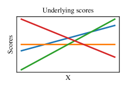
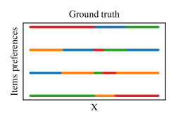
Figure 5: Ranking setting. We consider $\mathcal{X}$ an interval of $\mathbb{R}$, and $\mathcal{Y}=\mathfrak{S}_{m}$ with $m=4$ on the figure. (Right) To create a ranking dataset, we sample randomly $m$ lines in $\mathbb{R}^{2}$, embedding a value, or equivalently a score, associated to each items as a function of the input $x$. (Left) By ordering those lines, we create preferences between items as a function of $x$. On the figure, when $x$ is small, the “red” item is prefered over the “orange” item, itself prefered over the “blue” item, itself prefered over the “green” item. While when $x$ is big, “green” is prefered over “blue”, prefered over “orange”, prefered over “red”. We create a partial labelling dataset by sampling $(x_{i})\in\mathcal{X}^{n}$, and providing only partial ordering that the $(y_{i})$ follow. For example, for a small $x$, we might only give the partial information that “red” is prefered over “blue”.

D.2 Classification - Figure 2

Figure 2 corresponds to classification problems, based on real dataset from the LIBSVM datasets repository. At the time of writing, the datasets are available at https://www.csie.ntu.edu.tw/~cjlin/libsvmtools/datasets/multiclass.html. We present results on the “Dna” and “Svmguide2” datasets, that both have 3 classes ($m=3$), and respectively have 4000 samples with 180 features ($n=4000$,$d=180$) and 391 samples with 20 features ($n=391$, $d=20$).

In term of complexity, when $\mathcal{Y}=\left\llbracket 1,m\right\rrbracket=\left\{1,2,\cdots,m\right\}$, and weights based on kernel ridge regression with Gaussian kernel as described in the last paragraph the complexity of performing inference for Eqs. (5) and (13) can be done in $O(nm)$ in time and $O(n+m)$ in space, where $n$ is the number of training samples (Nowak-Vila et al., 2019; Cabannes et al., 2020). The disambiguation (4) performed with alternative minimization is done in $O(cn^{2}m)$ in time and in $O(n(n+m))$ in space, with $c$ the number of steps in the alternative minimization scheme. In practice, $c$ is really small, which can be understood since we are minimizing a concave function and each step leads to a guess on the border of the constraint domain.

Based on the dataset $(x_{i},y_{i})$, we create $(s_{i})$ by sampling it accordingly to $\gamma\delta_{\left\{y_{i}\right\}}+1-\gamma\delta_{\left\{y,y_{i}\right\}}$, with $y$ the most present labels in the dataset (indeed we choose the two datasets because they were not too big and presenting unequal labels proportion), and $\gamma\in[0,1]$ the corruption parameter represented in percentage on the $x$-axis of Figure 2. This skewed corruption allows to distinguish methods and invalidate the simple approach consisting to averaging candidate (AC) in set to recover $y_{i}$ from $s_{i}$, which works well when data are missing at random (Heitjan & Rubin, 1991). We separate $(x_{i},s_{i})$ in 8 folds, consider $\sigma\in d\cdot[1,.1,.01]$, where $d$ is the dimension of $\mathcal{X}$, and $\lambda\in n^{-1/2}\cdot[1,10^{-3},10^{-6}]$, where $n$ is the number of data. We test the different hyperparameter setup and reported the best error for each corruption parameter on Figure 2. Those errors are measured with the 0-1 loss, computed as averaged over the 8 folds, i.e. cross-validated, which standard deviation represented as errorbars on the figure. The best hyperparameter generally corresponds to $\sigma=.1$ and $\lambda=10^{-3}$ when the corruption is small and $\sigma=1$, $\lambda=10^{-3}$ when the corruption is big. Differences between cross-validated error and testing error were small, and we presented the first one out of simplicity.

In term of energy cost, the experiments were run on a personal laptop that has two processors, each of them running 2.3 billion instructions per second. During experiments, all the data were stored on the random access memory of 8GB. Experiments were run on Python, extensively relying on the NumPy library (Harris et al., 2020). The heaviest computation is Figure 2. Its total runtime, cross-validation included, was around 70 seconds. This paper is the results of experimentations, we evaluate the total cost of our experimentations to be three orders of magnitude higher than the cost of reproducing the final computations presented on Figure 1, 2 and 3. The total computational energy cost is very negligible.

D.3 Semi-supervised learning - Figure 3

On Figure 3, we review a semi-supervised classification problem with $\mathcal{Y}=\left\llbracket 1,4\right\rrbracket$, $\mathcal{X}=[-4.5,4.5]^{2}$, $\mu_{\mathcal{X}}$ only charging $\left\{x=(x_{1},x_{2})\in\mathbb{R}^{2}\,\middle|\,x_{1}^{2}+x_{2}^{2}\in\mathbb{N}^{*}\right\}$ and the solution $f^{*}:\mathcal{X}\to\mathcal{Y}$ being defined almost everywhere as $f^{*}(x)=x_{1}^{2}+x_{2}^{2}$. We collect a dataset $(x_{i},s_{i})$, by sampling 2000 points $\theta_{i}$ uniformly at random on $[0,1]$, as well as $r_{i}$ uniformly at random in $\left\llbracket 1,4\right\rrbracket=\left\{1,2,3,4\right\}$, before building $x_{i}=r_{i}\cdot(\cos(2\pi\theta_{i}),\sin(2\pi\theta_{i}))\in\mathcal{X}$, and $s_{i}=\mathcal{Y}$. We add four labelled points to this dataset $x_{2001}=(-2\sqrt{3},2)$ with $s_{2001}=\left\{4\right\}$, $x_{2001}=(1,-2\sqrt{2})$ with $s_{2002}=\left\{3\right\}$, $x_{2001}=(-\sqrt{3},-1)$ with $s_{2003}=\left\{2\right\}$ and $x_{2001}=(-1,0)$ with $s_{2004}=\left\{1\right\}$. We designed the weights $\alpha$ in Eq. (4) with $k$-nearest neighbors, with $k=20$, and solve this equation with a variant of alternative minimization, leading to the optimal solution $\tilde{y}_{i}=y_{i}^{*}$. In order to be able to compute the baseline (13), we design weights $\alpha$ for the inference task based on Nadaraya-Watson estimators with Gaussian kernel, defined as $\alpha_{i}(x)=\exp\left(\left\|x-x_{i}\right\|^{2}/h\right)$, with $h=.08$. We solve the inference task on a grid of $\mathcal{X}$ composed of 2500 points, and artificially recreate the observation to make them neat and reduce the resulting pdf size. Note that it is possible to design weights $\alpha$ that capture the cluster structure of the data, which, in this case, will lead to a nice behavior of the baseline as well as our algorithm. Arguably, this experiment showcase a regularization property of our algorithm (4).

D.4 Ranking with partial ordering

To conclude this experiment section, we look at ranking with partial ordering. We refer to Section 5.4 for a clear description of this instance of partial labelling. We provide to the reader eager to use our method, an implementation of our algorithm, available online at https://github.com/VivienCabannes/partial_labelling. It is based on LP relaxation of the NP-hard minimum feedback arcset problem. This relaxation was proven exact when $m\leq 6$ by Cabannes et al. (2020). The LP implementation relies on CPLEX (IBM, 2017). As complementary experiments, we will not provide much reproducibility details, those details would be really similar to the previous paragraphs, and the curious reader could run our code instead. We present our ranking setup on Figure 5 and our results on Figure 6.

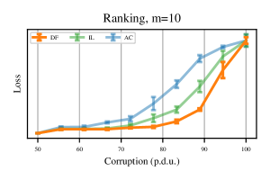
Figure 6: Performance of our algorithm for ranking with partial ordering. This figure is similar to Figure 2, but is based on the ranking problem illustrated on Figure 5. For this figure, we consider $m=10$, as it is arguably the limit where the LP relaxation provided by Cabannes et al. (2020) of the NP-hard minimum feedback arcset problem still performs well. The corruption parameter corresponds to the proportion of coordinates lost in the Kendall embedding when creating $s_{i}$ from $y_{i}$. Because the Kendall embedding satisfies transitivity constraints, a corruption smaller than 50% is almost ineffective to remove any information. In this figure, we observe a similar behavior for ranking to the one observed for classification on Figure 2, suggesting that those empirical findings are not spurious.

References

- Alayrac et al. (2016) Alayrac, J., Bojanowski, P., Agrawal, N., Sivic, J., Laptev, I., and Lacoste-Julien, S. Unsupervised learning from narrated instruction videos. In Conference on Computer Vision and Pattern Recognition, 2016.
- Audibert & Tsybakov (2007) Audibert, J.-Y. and Tsybakov, A. Fast learning rates for plug-in classifiers. Annals of Statistics, 2007.
- Bach & Harchaoui (2007) Bach, F. and Harchaoui, Z. DIFFRAC: a discriminative and flexible framework for clustering. In Neural Information Processing Systems 20, 2007.
- Bengio et al. (2006) Bengio, Y., Delalleau, O., and Roux, N. L. Label propagation and quadratic criterion. In Semi-Supervised Learning. MIT Press, 2006.
- Berthelot et al. (2019) Berthelot, D., Carlini, N., Goodfellow, I. J., Papernot, N., Oliver, A., and Raffel, C. Mixmatch: A holistic approach to semi-supervised learning. In Neural Information Processing Systems, 2019.
- Biau & Devroye (2015) Biau, G. and Devroye, L. Lectures on the Nearest Neighbor Method. Springer International Publishing, 2015.
- Boucheron et al. (2005) Boucheron, S., Bousquet, O., and Lugosi, G. Theory of classification: a survey of some recent advances. ESAIM: Probability and Statistics, 2005.
- Cabannes et al. (2020) Cabannes, V., Rudi, A., and Bach, F. Structured prediction with partial labelling through the infimum loss. In International Conference on Machine Learning, 2020.
- Cabannes et al. (2021) Cabannes, V., Rudi, A., and Bach, F. Fast rates in structured prediction. In Conference on Learning Theory, 2021.
- Cao et al. (2007) Cao, Z., Qin, T., Liu, T.-Y., Tsai, M.-F., and Li, H. Learning to rank: from pairwise approach to listwise approach. In International Conference of Machine Learning, 2007.
- Chang & Lin (2011) Chang, C. and Lin, C. LIBSVM: A library for support vector machines. ACM TIST, 2011.
- Cid-Sueiro et al. (2014) Cid-Sueiro, J., García-García, D., and Santos-Rodríguez, R. Consistency of losses for learning from weak labels. Lecture Notes in Computer Science, 2014.
- Ciliberto et al. (2016) Ciliberto, C., Rosasco, L., and Rudi, A. A consistent regularization approach for structured prediction. In Neural Information Processing Systems 29, 2016.
- Ciliberto et al. (2020) Ciliberto, C., Rosasco, L., and Rudi, A. A general framework for consistent structured prediction with implicit loss embeddings. Journal of Machine Learning Research, 2020.
- Cour et al. (2011) Cour, T., Sapp, B., and Taskar, B. Learning from partial labels. Journal of Machine Learning Research, 2011.
- Dabral et al. (2018) Dabral, R., Mundhada, A., Kusupati, U., Afaque, S., Sharma, A., and Jain, A. Learning 3D human pose from structure and motion. In European Conference on Computer Vision, 2018.
- Dempster et al. (1977) Dempster, A., Laird, N., and Rubin, D. Maximum likelihood from incomplete data via the EM algorithm. Journal of the Royal Statistical Society, 1977.
- Denoeux (2013) Denoeux, T. Maximum likelihood estimation from uncertain data in the belief function framework. IEEE Transactions on Knowledge and Data Engineerin, 2013.
- Doersch & Zisserman (2017) Doersch, C. and Zisserman, A. Multi-task self-supervised visual learning. In International Conference on Computer Vision, 2017.
- Duchi et al. (2010) Duchi, J. C., Mackey, L. W., and Jordan, M. I. On the consistency of ranking algorithms. In International Conference on Machine Learning, 2010.
- Duda et al. (2000) Duda, R., Hart, P., and Stork, D. Pattern Classification, 2nd Edition. Wiley, 2000.
- Dulac-Arnold et al. (2019) Dulac-Arnold, G., Zeghidour, N., Cuturi, M., Beyer, L., and Vert, J.-P. Deep multiclass learning from label proportions. In ArXiv, 2019.
- Gong et al. (2018) Gong, C., Liu, T., Tang, Y., Yang, J., Yang, J., and Tao, D. A regularization approach for instance-based superset label learning. IEEE Transactions on Cybernetics, 2018.
- Harris et al. (2020) Harris, C., Millman, J., van der Walt, S., et al. Array programming with NumPy. Nature, 2020.
- Hein et al. (2007) Hein, M., Audibert, J.-Y., and von Luxburg, U. Graph Laplacians and their convergence on random neighborhood graphs. Journal of Machine Learning Research, 2007.
- Heitjan & Rubin (1991) Heitjan, D. and Rubin, D. Ignorability and coarse data. The Annals of Statistics, 1991.
- Hüllermeier (2014) Hüllermeier, E. Learning from imprecise and fuzzy observations: Data disambiguation through generalized loss minimization. International Journal of Approximate Reasoning, 2014.
- Hüllermeier et al. (2008) Hüllermeier, E., Fürnkranz, J., Cheng, W., and Brinker, K. Label ranking by learning pairwise preferences. Artificial Intelligence, 2008.
- IBM (2017) IBM. IBM ILOG CPLEX 12.7 User’s Manual. IBM ILOG CPLEX Division, 2017.
- Jia et al. (2018) Jia, Y., Zhang, Y., Weiss, R., Wang, Q., Shen, J., Ren, F., Chen, Z., Nguyen, P., Pang, R., Lopez-Moreno, I., and Wu, Y. Transfer learning from speaker verification to multispeaker text-to-speech synthesis. In Neural Information Processing Systems, 2018.
- Jin & Ghahramani (2002) Jin, R. and Ghahramani, Z. Learning with multiple labels. In Neural Information Processing Systems, 2002.
- Joulin et al. (2010) Joulin, A., Bach, F., and Ponce, J. Discriminative clustering for image co-segmentation. In Conference on Computer Vision and Pattern Recognition, 2010.
- Kendall (1938) Kendall, M. A new measure of rank correlation. Biometrika, 1938.
- Korba et al. (2018) Korba, A., Garcia, A., and d’Alché-Buc, F. A structured prediction approach for label ranking. In Neural Information Processing Systems, 2018.
- Lienen & Hüllermeier (2021) Lienen, J. and Hüllermeier, E. From label smoothing to label relaxation. In AAAI Conference on Artificial Intelligence, 2021.
- Liu & Dietterich (2014) Liu, L.-P. and Dietterich, T. Learnability of the superset label learning problem. In International Conference on Machine Learning, 2014.
- Luo & Orabona (2010) Luo, J. and Orabona, F. Learning from candidate labeling sets. In Neural Information Processing Systems, 2010.
- Miech et al. (2019) Miech, A., Zhukov, D., Alayrac, J.-B., Tapaswi, M., Laptev, I., and Sivic, J. Howto100m: Learning a text-video embedding by watching hundred million narrated video clips. In International Conference on Computer Vision, 2019.
- Muzellec et al. (2020) Muzellec, B., Josse, J., Boyer, C., and Cuturi, M. Missing data imputation using optimal transport. In International Conference of Machine Learning, 2020.
- Nowak-Vila et al. (2019) Nowak-Vila, A., Bach, F., and Rudi, A. Sharp analysis of learning with discrete losses. In Artificial Intelligence and Statistics, 2019.
- Papandreou et al. (2015) Papandreou, G., Chen, L.-C., Murphy, K., and Yuille, A. Weakly- and semi-supervised learning of a deep convolutional network for semantic image segmentation. In International Conference on Computer Vision, 2015.
- Perchet & Quincampoix (2015) Perchet, V. and Quincampoix, M. On a unified framework for approachability with full or partial monitoring. Mathematics of Operations Research, 2015.
- Quadrianto et al. (2009) Quadrianto, N., Smola, A., Caetano, T., and Le, Q. V. Estimating labels from label proportions. Journal of Machine Learning Research, 2009.
- Rigollet (2007) Rigollet, P. Generalization error bounds in semi-supervised classification under the cluster assumption. Journal of Machine Learning Research, 2007.
- Rubin (1976) Rubin, D. Inference and missing data. Biometrika, 1976.
- Sheppard (1897) Sheppard, W. On the calculation of the most probable values of frequency constants, for data arranged according to equidistant division of a scale. Proceedings of the London Mathematical Society, 1897.
- Steinwart & Christmann (2008) Steinwart, I. and Christmann, A. Support vector machines. Springer Science & Business Media, 2008.
- Stone (1977) Stone, C. Consistent nonparametric regression. The Annals of Statistics, 1977.
- Tobin (1958) Tobin, J. Estimation of relationships for limited dependent variables. Econometrica, 1958.
- van Rooyen & Williamson (2017) van Rooyen, B. and Williamson, R. C. A theory of learning with corrupted labels. Journal of Machine Learning Research, 2017.
- Vapnik (1995) Vapnik, V. The Nature of Statistical Learning Theory. Springer-Verlag, 1995.
- Wang et al. (2017) Wang, L., Lu, H., Wang, Y., Feng, M., Wang, D., Yin, B., and Ruan, X. Learning to detect salient objects with image-level supervision. In Conference on Computer Vision and Pattern Recognition, 2017.
- Wei et al. (2021) Wei, C., Shen, K., Chen, Y., and Ma, T. Theoretical analysis of self-training with deep networks on unlabeled data. In International Conference on Learning Representations, 2021.
- Xu et al. (2004) Xu, L., Neufeld, J., Larson, B., and Schuurmans, D. Maximum margin clustering. Neural Information Processing Systems, 2004.
- Zhou et al. (2003) Zhou, D., Bousquet, O., Lal, T. N., Weston, J., and Schölkopf, B. Learning with local and global consistency. In Neural Information Processing Systems, 2003.
- Zhu et al. (2003) Zhu, X., Ghahramani, Z., and Lafferty, J. D. Semi-supervised learning using Gaussian fields and harmonic functions. In International Conference of Machine Learning, 2003.