Abstract

We study the temporal evolution of the circuit complexity for a subsystem in harmonic lattices after a global quantum quench of the mass parameter, choosing the initial reduced density matrix as the reference state. Upper and lower bounds are derived for the temporal evolution of the complexity for the entire system. The subsystem complexity is evaluated by employing the Fisher information geometry for the covariance matrices. We discuss numerical results for the temporal evolutions of the subsystem complexity for a block of consecutive sites in harmonic chains with either periodic or Dirichlet boundary conditions, comparing them with the temporal evolutions of the entanglement entropy. For infinite harmonic chains, the asymptotic value of the subsystem complexity is studied through the generalised Gibbs ensemble.

1 Introduction

The complexity of a quantum circuit is a quantity introduced in quantum information theory [1, 2, 3, 4, 5, 6] which has been studied also in the context of the holographic correspondence during the past few years [7, 8, 9, 10, 11, 12, 13, 14, 15, 16]; hence it provides an insightful way to explore a connection between quantum information theory and quantum gravity.

A quantum circuit allows to construct a target state starting from a reference state through a sequence of gates. The circuit complexity quantifies the difficulty to obtain the target state from the reference state by counting the minimum number of allowed gates that is necessary to construct the circuit in an optimal way. Besides the reference state, the target state and the set of allowed gates, the circuit complexity can depend also on the tolerance parameter for the target state. Many results have been obtained for the complexity of quantum circuits made by pure states constructed through lattice models [17, 18, 19, 20, 21, 22, 23, 24, 25] and in the gravitational side of the holographic correspondence. Some proposals have been done also to study the circuit complexity in quantum fields theories [26, 27, 28, 29, 30, 31, 32, 33, 34, 35, 36, 37, 38].

Quantum quenches are insightful ways to explore the dynamics of isolated quantum systems out of equilibrium (see [39, 40] for recent reviews). Given a quantum system prepared in the ground state $|\psi_{0}\rangle$ of the hamiltonian $\widehat{H}_{0}$, at $t=0$ a sudden change is performed such that the evolution Hamiltonian of the initial state $|\psi_{0}\rangle$ becomes $\widehat{H}\neq\widehat{H}_{0}$. Since $\widehat{H}$ and $\widehat{H}_{0}$ do not commute in general, the unitary evolution $|\psi(t)\rangle=e^{-\textrm{i}\widehat{H}t}|\psi_{0}\rangle$ for $t>0$ is highly non trivial. In the typical global quench, a parameter occurring in the Hamiltonian is suddenly changed from its value $\omega_{0}$ in $\widehat{H}_{0}$ to the value $\omega$ in $\widehat{H}$ [41, 42, 43, 39]. Insightful results have been obtained about the asymptotic regime $t\to\infty$ of this unitary evolution by employing the generalised Gibbs ensemble (GGE) (see the reviews [44, 45, 46]).

It is worth studying the circuit complexity with the target state given by the time-evolved pure state of certain unitary evolution and the reference state by another pure state along the same evolution [47, 48, 49, 18, 50]. In particular, considering a global quench protocol, we are interested in the optimal circuit and in the corresponding complexity where $|\psi(t)\rangle$ and $|\psi_{0}\rangle$ are respectively the target and the reference states. Within the gauge/gravity correspondence, the temporal evolution of complexity for pure states has been explored in [51, 52, 53].

Entanglement of spatial bipartitions plays a crucial role both in quantum information theory and in quantum gravity, hence it is a fundamental tool to understand the connections between them (see [54, 55, 56, 57, 58, 59, 60] for reviews). The entanglement dynamics after global quantum quenches has been largely explored by considering the temporal evolutions of various entanglement quantifiers. The entanglement entropy has been mainly investigated through various methods [61, 62, 63, 40, 64, 65], but also other entanglement quantifiers like the entanglement spectra [66, 67, 68], the entanglement Hamiltonians [66, 69, 67], the entanglement negativity [70] and the entanglement contours [71, 72, 67] have been explored.

In order to understand the relation between entanglement and complexity, it is useful to study the optimal circuits and the corresponding circuit complexity when both the reference and the target states are mixed states [73, 74, 75, 76]. The approach to the complexity of mixed states based on the purification complexity [77, 73, 76] is general, but evaluating this quantity for large systems is technically complicated. Some explicit results for large systems can be found by restricting to the simple case of bosonic Gaussian states and by employing the methods of the information geometry [78, 79, 80]. In our analysis we adopt the approach to the complexity of mixed states based on the Fisher information geometry [74], which allows to study large systems numerically. The crucial assumption underlying this approach is that all the states involved in the construction of the circuit are Gaussian. We consider the important special case given by the subsystem complexity, namely the circuit complexity corresponding to a circuit where both the reference and the target states are the reduced density matrices associated to a subsystem.

Within the gauge/gravity correspondence, the subsystem complexity has been evaluated both in static [12, 16, 81, 77, 82, 83] and in time dependent gravitational backgrounds [84, 85, 86, 87]. In static backgrounds, it is given by the volume identified by the minimal area hypersurface anchored to the boundary of the subsystem, whose area provides the holographic entanglement entropy [88] (for static black holes, this hypersurface does not cross the horizon [89, 90, 91]), while, in time dependent gravitational spacetimes, the extremal hypersurface occurring in the covariant proposal for the holographic entanglement entropy [64] must be employed.

In this manuscript we study the temporal evolution of the subsystem complexity after a global quantum quench in harmonic lattices where the mass parameter is suddenly changed from $\omega_{0}$ to $\omega$. Considering a ground state as the initial state, the Gaussian nature of the state is preserved during the temporal evolution. In these bosonic systems, the reduced density matrices are characterised by the corresponding reduced covariance matrices [92]. By employing the approach to the complexity of bosonic mixed Gaussian states based on the Fisher information geometry [74], we evaluate numerically the subsystem complexity for one-dimensional harmonic lattices (i.e. harmonic chains) and subsystems $A$ given by blocks of consecutive sites. We consider harmonic chains where either periodic boundary conditions (PBC) or Dirichlet boundary conditions (DBC) are imposed. This allows to study the role of the zero mode. The temporal evolution of the subsystem complexity at a generic time after the global quench w.r.t. the initial state is compared with the temporal evolution of the corresponding increment of the entanglement entropy.

This manuscript is organised as follows. In Sec. 2 we introduce the main expressions to evaluate the circuit complexity after the global quench of the mass parameter through the covariance matrices of the reference and the target states for harmonic lattices in a generic number of dimensions. In the special case where the entire system is considered, these states are pure and bounds are obtained for the temporal evolution of the circuit complexity w.r.t. the initial state. In Sec. 3 we specify this analysis to harmonic chains with either PBC or DBC. The main results of this manuscript are discussed in Sec. 4 and Sec. 5, where the temporal evolution of the subsystem complexity for a block of consecutive sites is investigated. In Sec. 4, finite harmonic chains with either PBC or DBC are studied, while in Sec. 5 we consider infinite harmonic chains either on the line or on the semi-infinite line with DBC at the origin. In the cases of infinite chains, we employ known results about the GGE to determine the asymptotic regime of the subsystem complexity. In Sec. 6 we draw some conclusions. Some technical details and supplementary results are discussed in the appendices A, B, C and D.

2 Complexity from the covariance matrix after the quench

In this section we discuss the expressions that allow to evaluate the temporal evolution of the circuit complexity based on the Fisher-Rao geometry for the harmonic lattices in a generic number of spatial dimensions when both the reference and the target states are pure. Analytic expressions that bound this temporal evolution are also derived.

2.1 Covariance matrix after the quench

The Hamiltonian of the harmonic lattice made by $N$ sites with nearest neighbour spring-like interaction reads

$$\widehat{H}\,=\,\sum_{i=1}^{N}\left(\frac{1}{2m}\,\hat{p}_{i}^{2}+\frac{m\omega^{2}}{2}\,\hat{q}_{i}^{2}\right)+\sum_{\langle i,j\rangle}\frac{\kappa}{2}(\hat{q}_{i}-\hat{q}_{j})^{2}\,=\,\frac{1}{2}\,\hat{\boldsymbol{r}}^{\textrm{t}}H^{\textrm{\tiny phys}}\,\hat{\boldsymbol{r}}$$ (2.1)

where the position and the momentum operators $\hat{q}_{i}$ and $\hat{p}_{i}$ are hermitean operators satisfying the canonical commutation relations $[\hat{q}_{i},\hat{q}_{j}]=[\hat{p}_{i},\hat{p}_{j}]=0$ and $[\hat{q}_{i},\hat{p}_{j}]=\textrm{i}\delta_{i,j}$. The matrix $H^{\textrm{\tiny phys}}$ in (2.1) has been defined by collecting the position and the momentum operators into the vector $\hat{\boldsymbol{r}}\equiv(\hat{q}_{1},\dots,\hat{q}_{N},\hat{p}_{1},\dots,\hat{p}_{N})^{\textrm{t}}$.

In the Heisenberg picture, the unitary temporal evolution of the position and the momentum operators $\hat{q}_{j}(t)$ and $\hat{p}_{j}(t)$ through the evolution Hamiltonian $\widehat{H}$ reads

$$\hat{q}_{j}(t)=e^{\textrm{i}\widehat{H}t}\hat{q}_{j}(0)e^{-\textrm{i}\widehat{H}t}\qquad\hat{p}_{j}(t)=e^{\textrm{i}\widehat{H}t}\hat{p}_{j}(0)e^{-\textrm{i}\widehat{H}t}\,.$$ (2.2)

In order to study the temporal evolution of the harmonic lattices after the global quantum quench of the mass parameter that we are considering, we need to introduce the $N\times N$ correlation matrices for operators (2.2) whose elements read

$$\begin{array}[]{l}Q_{i,j}(t)\equiv\langle\psi_{0}|\,\hat{q}_{i}(t)\,\hat{q}_{j}(t)\,|\psi_{0}\rangle\\ \rule{0.0pt}{17.07182pt}P_{i,j}(t)\equiv\langle\psi_{0}|\,\hat{p}_{i}(t)\,\hat{p}_{j}(t)\,|\psi_{0}\rangle\\ \rule{0.0pt}{17.07182pt}M_{i,j}(t)\equiv\textrm{Re}\big{[}\langle\psi_{0}|\,\hat{q}_{i}(t)\,\hat{p}_{j}(t)\,|\psi_{0}\rangle\big{]}\end{array}$$ (2.3)

where $|\psi_{0}\rangle$ is the ground state of the Hamiltonian $\widehat{H}_{0}$, defined by (2.1) with $\omega$ replaced by $\omega_{0}$.

At any time $t>0$ after the quench, the system is completely characterised by its covariance matrix $\gamma(t)$, which is the following $2N\times 2N$ real, symmetric and positive definite matrix

$$\gamma(t)=\,\bigg{(}\begin{array}[]{cc}Q(t)&M(t)\\ M(t)^{\textrm{t}}&P(t)\\ \end{array}\bigg{)}$$ (2.4)

where the elements of the $N\times N$ block matrices are given by (2.3). This covariance matrix has been already used to study the entanglement dynamics e.g. in [61, 70, 62].

In the appendix A.1 we discuss the fact that, for the global quench we are exploring, the blocks of the covariance matrix (2.4) can be decomposed as

$$Q(t)=\widetilde{V}\,\mathcal{Q}(t)\,\widetilde{V}^{\textrm{t}}\,\,\qquad\rule{0.0pt}{17.07182pt}P(t)=\widetilde{V}\,\mathcal{P}(t)\,\widetilde{V}^{\textrm{t}}\,\,\qquad\rule{0.0pt}{17.07182pt}M(t)=\widetilde{V}\,\mathcal{M}(t)\,\widetilde{V}^{\textrm{t}}$$ (2.5)

where $\widetilde{V}$ is a real orthogonal $N\times N$ matrix, while $\mathcal{Q}(t)$, $\mathcal{P}(t)$ and $\mathcal{M}(t)$ are $N\times N$ diagonal matrices whose $k$-th element along the diagonal is [43]

$$\begin{array}[]{l}\displaystyle Q_{k}(t)\equiv\mathcal{Q}_{k,k}(t)=\frac{1}{2m\Omega_{k}}\left(\,\frac{\Omega_{k}}{\Omega_{0,k}}\,[\cos(\Omega_{k}t)]^{2}+\frac{\Omega_{0,k}}{\Omega_{k}}\,[\sin(\Omega_{k}t)]^{2}\right)\\ \displaystyle\rule{0.0pt}{25.6073pt}P_{k}(t)\equiv\mathcal{P}_{k,k}(t)=\frac{m\Omega_{k}}{2}\left(\,\frac{\Omega_{k}}{\Omega_{0,k}}\,[\sin(\Omega_{k}t)]^{2}+\frac{\Omega_{0,k}}{\Omega_{k}}\,[\cos(\Omega_{k}t)]^{2}\right)\\ \displaystyle\rule{0.0pt}{25.6073pt}M_{k}(t)\equiv\mathcal{M}_{k,k}(t)=\frac{1}{2}\left(\frac{\Omega_{0,k}}{\Omega_{k}}-\,\frac{\Omega_{k}}{\Omega_{0,k}}\right)\sin(\Omega_{k}t)\cos(\Omega_{k}t)\end{array}$$ (2.6)

in terms of the dispersion relations $\Omega_{0,k}$ and $\Omega_{k}$ of the Hamiltonians $\widehat{H}_{0}$ and $\widehat{H}$ respectively, which depend both on the dimensionality of the lattice and on the boundary conditions.

At $t=0$, the expressions in (2.6) simplify respectively to

$$Q_{k}(0)=\frac{1}{2m\,\Omega_{0,k}}\;\;\qquad\;\;P_{k}(0)=\frac{m\,\Omega_{0,k}}{2}\;\;\qquad\;\;M_{k}(0)=0\,.$$ (2.7)

From the above discussion, one realises that $\gamma(t)$ is a function of $t$ determined by the set of parameters given by $\{m,\kappa,\omega,\omega_{0}\}$.

When the dispersion relation vanishes for certain value of $k$, e.g. $k=N$, the corresponding mode is a zero mode. The relations (2.6) and (2.7) are well defined when $\Omega_{0,k}$ does not vanish; hence $\Omega_{k}$ can have a zero mode, while $\Omega_{0,k}$ cannot. This highlights the asymmetric role of $\Omega_{0,k}$ and $\Omega_{k}$.

2.2 Complexity for the system

The circuit complexity is proportional to the length of the optimal quantum circuit that creates a target state from a reference state. In this manuscript we evaluate the complexity through the Fisher-Rao distance between two bosonic Gaussian states with vanishing first moments [92, 93, 94]. This approach allows to study also the circuits made by mixed states [74].

Denoting by $\gamma_{\textrm{\tiny R}}$ and $\gamma_{\textrm{\tiny T}}$ the covariance matrices with vanishing first moments of the reference and of the target state respectively, the Fisher-Rao distance between them [79, 95] provides the following definition of complexity

$$\mathcal{C}\,\equiv\,\frac{1}{2\sqrt{2}}\;\sqrt{\,\textrm{Tr}\,\Big{\{}\big{[}\log\big{(}\gamma_{\textrm{\tiny T}}\,\gamma_{\textrm{\tiny R}}^{-1}\big{)}\big{]}^{2}\Big{\}}}\;.$$ (2.8)

When both $\gamma_{\textrm{\tiny R}}$ and $\gamma_{\textrm{\tiny T}}$ characterise pure states, this complexity corresponds to the one defined through the $F_{2}$ cost function [18].

The analysis of the circuits made by bosonic Gaussian states based on the Fisher-Rao metric provides also the optimal circuit between $\gamma_{\textrm{\tiny R}}$ and $\gamma_{\textrm{\tiny T}}$. It reads [95]

$$G_{s}(\gamma_{\textrm{\tiny R}}\,,\gamma_{\textrm{\tiny T}})\,\equiv\,\gamma_{\textrm{\tiny R}}^{1/2}\Big{(}\gamma_{\textrm{\tiny R}}^{-1/2}\,\gamma_{\textrm{\tiny T}}\,\gamma_{\textrm{\tiny R}}^{-1/2}\Big{)}^{s}\gamma_{\textrm{\tiny R}}^{1/2}\;\;\qquad\;\;0\leqslant s\leqslant 1$$ (2.9)

which gives $\gamma_{\textrm{\tiny R}}$ when $s=0$ and $\gamma_{\textrm{\tiny T}}$ when $s=1$. The length of the optimal circuit (2.9) evaluated through the Fisher-Rao distance is proportional to the circuit complexity (2.8), which has been explored both for pure states [18] and for mixed states [74].

In this manuscript we are interested in the temporal evolution of the circuit complexity after a global quench. In the following discussion and in Sec. 3 we consider first the case where both the reference and the target states are pure states, while in Sec. 4 and Sec. 5 we study the case where both the reference and the target states are mixed states.

Denoting by $t_{\textrm{\tiny R}}$ and $t_{\textrm{\tiny T}}$ the values of $t$ corresponding to the reference state and to the target state respectively, let us adopt the following notation

$$\gamma_{\textrm{\tiny R}}=\gamma(t_{\textrm{\tiny R}})\;\;\qquad\;\;\gamma_{\textrm{\tiny T}}=\gamma(t_{\textrm{\tiny T}})\,.$$ (2.10)

In the most general setup, $\gamma_{\textrm{\tiny R}}$ is a function of $t_{\textrm{\tiny R}}$ characterised by the set of parameters $\{m_{\textrm{\tiny R}},\kappa_{\textrm{\tiny R}},\omega_{\textrm{\tiny R}},\omega_{0,\textrm{\tiny R}}\}$, while $\gamma_{\textrm{\tiny T}}$ is a function of $t_{\textrm{\tiny T}}$ parameterised by $\{m_{\textrm{\tiny T}},\kappa_{\textrm{\tiny T}},\omega_{\textrm{\tiny T}},\omega_{0,\textrm{\tiny T}}\}$. This means that the reference and target states are obtained as the time-evolved states at $t=t_{\textrm{\tiny R}}\geqslant 0$ and $t=t_{\textrm{\tiny T}}\geqslant t_{\textrm{\tiny R}}$ respectively, through two different global quenches determined by $\{\kappa_{\textrm{\tiny R}},m_{\textrm{\tiny R}},\omega_{\textrm{\tiny R}},\omega_{0,\textrm{\tiny R}}\}$ and $\{\kappa_{\textrm{\tiny T}},m_{\textrm{\tiny T}},\omega_{\textrm{\tiny T}},\omega_{0,\textrm{\tiny T}}\}$ respectively.

The covariance matrix (2.4) at a generic value of $t$ can be written as follows

$$\gamma(t)=V^{\textrm{t}}\,\Gamma(t)\,V\,\,\qquad\,\,V=\widetilde{V}\oplus\widetilde{V}$$ (2.12)

where $V$ is an orthogonal and symplectic matrix because $\widetilde{V}$ is orthogonal and the block decomposition of $\Gamma(t)$ reads

$$\Gamma(t)=\bigg{(}\begin{array}[]{cc}\mathcal{Q}(t)&\!\,\,\mathcal{M}(t)\\ \mathcal{M}(t)&\!\,\,\mathcal{P}(t)\end{array}\bigg{)}$$ (2.13)

in terms of the diagonal matrices whose elements have been defined in (2.6).

Hereafter we enlighten the expressions by avoiding to indicate explicitly the dependence on $t$, wherever this is possible. The inverse of (2.13) is

$$\Gamma^{-1}=\big{(}\mathcal{Q}\,\mathcal{P}-\mathcal{M}^{2}\big{)}^{-1}\bigg{(}\begin{array}[]{cc}\mathcal{P}\!&-\,\mathcal{M}\\ -\,\mathcal{M}\!&\mathcal{Q}\end{array}\bigg{)}\,.$$ (2.15)

Since $\gamma$ in (2.4) describes a pure state, the condition $(\textrm{i}J\gamma)^{2}=\tfrac{1}{4}\,\boldsymbol{1}$ holds; hence the blocks $\mathcal{Q}$, $\mathcal{P}$ and $\mathcal{M}$ are not independent. More explicitly, this constraint reads

$$(\textrm{i}J\gamma)^{2}=\bigg{(}\begin{array}[]{cc}PQ-(M^{\textrm{t}})^{2}&PM-M^{\textrm{t}}P\\ QM^{\textrm{t}}-MQ&QP-M^{2}\end{array}\bigg{)}=\,V^{\textrm{t}}\,\bigg{(}\begin{array}[]{cc}\mathcal{P}\mathcal{Q}-\mathcal{M}^{2}&\mathcal{P}\mathcal{M}-\mathcal{M}^{\textrm{t}}\mathcal{P}\\ \mathcal{Q}\mathcal{M}^{\textrm{t}}-\mathcal{M}\mathcal{Q}&\mathcal{Q}\,\mathcal{P}-\mathcal{M}^{2}\end{array}\bigg{)}\,V=\frac{1}{4}\,\boldsymbol{1}$$ (2.16)

which implies

$$\mathcal{Q}\,\mathcal{P}-\mathcal{M}^{2}=\frac{1}{4}\,\boldsymbol{1}\qquad\Longleftrightarrow\qquad Q_{k}P_{k}-M_{k}^{2}=\frac{1}{4}\;\qquad\;1\leqslant k\leqslant N\,.$$ (2.17)

This result allows to further simplify (2.15), which becomes

$$\Gamma^{-1}=\,4\,\bigg{(}\begin{array}[]{cc}\mathcal{P}&-\mathcal{M}\\ -\mathcal{M}&\mathcal{Q}\end{array}\bigg{)}\,.$$ (2.18)

In this manuscript we restrict to cases where a symplectic matrix $V$ exists such that

$$\gamma_{\textrm{\tiny R}}=V^{\textrm{t}}\,\Gamma_{\textrm{\tiny R}}\,V\;\;\qquad\;\;\gamma_{\textrm{\tiny T}}=V^{\textrm{t}}\,\Gamma_{\textrm{\tiny T}}\,V$$ (2.19)

where both $\Gamma_{\textrm{\tiny R}}$ and $\Gamma_{\textrm{\tiny T}}$ have the form (2.13), in terms of the corresponding diagonal matrices. When (2.19) holds, the matrix occurring in the argument of the logarithm in (2.8) becomes

$$\gamma_{\textrm{\tiny T}}\,\gamma_{\textrm{\tiny R}}^{-1}=V^{\textrm{t}}\,\Gamma_{\textrm{\tiny T}}\,\Gamma_{\textrm{\tiny R}}^{-1}\,V^{-\textrm{t}}$$ (2.20)

which tells us that the complexity (2.8) is provided by the eigenvalues of $\Gamma_{\textrm{\tiny T}}\,\Gamma_{\textrm{\tiny R}}^{-1}$. Thus, the matrix $V$ does not influence the temporal evolution of the complexity after the global quench when both the reference and the target states are pure states. Instead, they play a crucial role for the temporal evolution of the subsystem complexity discussed in Sec. 4 and Sec. 5.

By using (2.13) for $\Gamma_{\textrm{\tiny T}}$ and (2.18) for $\Gamma^{-1}_{\textrm{\tiny R}}$, we obtain the following block matrix

$$\Gamma_{\textrm{\tiny T}}\,\Gamma^{-1}_{\textrm{\tiny R}}=4\,\bigg{(}\begin{array}[]{cc}\mathcal{P}_{\textrm{\tiny R}}\mathcal{Q}_{\textrm{\tiny T}}-\mathcal{M}_{\textrm{\tiny R}}\mathcal{M}_{\textrm{\tiny T}}&\;\;\mathcal{Q}_{\textrm{\tiny R}}\mathcal{M}_{\textrm{\tiny T}}-\mathcal{M}_{\textrm{\tiny R}}\mathcal{Q}_{\textrm{\tiny T}}\\ \mathcal{P}_{\textrm{\tiny R}}\mathcal{M}_{\textrm{\tiny T}}-\mathcal{M}_{\textrm{\tiny R}}\mathcal{P}_{\textrm{\tiny T}}&\;\;\mathcal{Q}_{\textrm{\tiny R}}\mathcal{P}_{\textrm{\tiny T}}-\mathcal{M}_{\textrm{\tiny R}}\mathcal{M}_{\textrm{\tiny T}}\end{array}\bigg{)}$$ (2.21)

whose blocks are diagonal matrices. By using also (2.17), for the eigenvalues of (2.21) we find

$$g_{\textrm{\tiny TR},k}^{(\pm)} \equiv 2\bigg{(}P_{\textrm{\tiny R},k}Q_{\textrm{\tiny T},k}+Q_{\textrm{\tiny R},k}P_{\textrm{\tiny T},k}-2M_{\textrm{\tiny R},k}M_{\textrm{\tiny T},k}$$

$$\hskip 17.07182pt\pm\,\sqrt{\big{(}P_{\textrm{\tiny R},k}Q_{\textrm{\tiny T},k}-Q_{\textrm{\tiny R},k}P_{\textrm{\tiny T},k}\big{)}^{2}+4\big{(}Q_{\textrm{\tiny R},k}M_{\textrm{\tiny T},k}-M_{\textrm{\tiny R},k}Q_{\textrm{\tiny T},k}\big{)}\big{(}P_{\textrm{\tiny R},k}M_{\textrm{\tiny T},k}-M_{\textrm{\tiny R},k}P_{\textrm{\tiny T},k}\big{)}}\;\bigg{)}$$

labelled by $1\leqslant k\leqslant N$, which can be written as

$$g_{\textrm{\tiny TR},k}^{(\pm)}=C_{\textrm{\tiny TR},k}\pm\sqrt{C_{\textrm{\tiny TR},k}^{2}-1}$$ (2.25)

where

$$C_{\textrm{\tiny TR},k}\equiv 2\big{(}Q_{\textrm{\tiny T},k}\,P_{\textrm{\tiny R},k}+P_{\textrm{\tiny T},k}\,Q_{\textrm{\tiny R},k}-2\,M_{\textrm{\tiny T},k}\,M_{\textrm{\tiny R},k}\big{)}$$ (2.26)

in terms of the expressions in (2.6) specialised to the reference and the target states.

From (2.25) and (2.26), one observes that

$$g_{\textrm{\tiny TR},k}^{(+)}\,g_{\textrm{\tiny TR},k}^{(-)}=16\big{(}Q_{\textrm{\tiny R},k}P_{\textrm{\tiny R},k}-M_{\textrm{\tiny R},k}^{2}\big{)}\big{(}Q_{\textrm{\tiny T},k}P_{\textrm{\tiny T},k}-M_{\textrm{\tiny T},k}^{2}\big{)}\,.$$ (2.27)

By employing (2.17) in this result, we find $g_{\textrm{\tiny TR},k}^{(+)}=1/g_{\textrm{\tiny TR},k}^{(-)}$ for pure states, for any $1\leqslant k\leqslant N$.

From (2.21), (2.25) and (2.27), for the complexity (2.8) one obtains

$$\mathcal{C}\,=\,\frac{1}{2}\,\sqrt{\sum_{k=1}^{N}\!\big{[}\log(g_{\textrm{\tiny TR},k}^{(+)})\big{]}^{2}}\,=\,\frac{1}{2}\,\sqrt{\sum_{k=1}^{N}\!\big{[}\log(g_{\textrm{\tiny TR},k}^{(-)})\big{]}^{2}}\,=\,\frac{1}{2}\,\sqrt{\sum_{k=1}^{N}\!\big{[}\textrm{arccosh}(C_{\textrm{\tiny TR},k})\big{]}^{2}}\;.$$ (2.28)

In the most general setup described below (2.10), the complexity can be found by writing (2.6) for the reference and the target states first and then and plugging the results into (2.26) and (2.28). The final result is a complicated expressions which can be seen as a function of $t_{\textrm{\tiny R}}$ and $t_{\textrm{\tiny T}}$ parameterised by $\{\kappa_{\textrm{\tiny R}},m_{\textrm{\tiny R}},\omega_{\textrm{\tiny R}},\omega_{0,\textrm{\tiny R}}\}$ and $\{\kappa_{\textrm{\tiny T}},m_{\textrm{\tiny T}},\omega_{\textrm{\tiny T}},\omega_{0,\textrm{\tiny T}}\}$. We remark that (2.28) can be employed when (2.19) holds. Furthermore, we consider only cases where the matrix $V$ in (2.19) depends on the geometric parameters of the system and of the subsystem but it is independent of the physical parameters occurring in the Hamiltonians (see Sec. 3.1).

In the appendix A.2, the expression (2.28) is obtained through the Williamson’s decomposition [96] of the covariance matrices (2.10).

A remarkable simplification occurs when the reference and the target states are pure states along the time evolution of a given quench. In this case, the parameters to fix in (2.6) are $m_{\textrm{\tiny R}}=m_{\textrm{\tiny T}}=m$, $\kappa_{\textrm{\tiny R}}=\kappa_{\textrm{\tiny T}}=\kappa$, $\omega_{\textrm{\tiny R}}=\omega_{\textrm{\tiny T}}=\omega$, and $\omega_{0,\textrm{\tiny R}}=\omega_{0,\textrm{\tiny T}}=\omega_{0}$; hence (2.26) simplifies to

$$C_{\textrm{\tiny TR},k}=1+\frac{1}{2}\Bigg{(}\frac{\Omega_{k}^{2}-\Omega^{2}_{0,k}}{\Omega_{k}\,\Omega_{0,k}}\,\sin[\Omega_{k}(t_{\textrm{\tiny R}}-t_{\textrm{\tiny T}})]\Bigg{)}^{2}$$ (2.29)

which must be plugged into (2.28) to get the complexity of pure states after the global quench. Notice that (2.29) is not invariant under the exchange $\Omega_{k}\leftrightarrow\Omega_{0,k}$ for a given $k$. We remark that (2.29) and the corresponding complexity depend on $|t_{\textrm{\tiny R}}-t_{\textrm{\tiny T}}|$. This is not the case for the most generic choice of the parameters.

2.3 Complexity with respect to the initial state

A very natural choice for the reference state is the initial state $|\psi_{0}\rangle$, which is a crucial ingredient of the quench protocol. This corresponds to choose $t_{\textrm{\tiny R}}=0$ in (2.10). In this case, from (2.7) and (2.17) we have that $\mathcal{M}_{\textrm{\tiny R}}=\boldsymbol{0}$ and $\mathcal{Q}_{\textrm{\tiny R}}\mathcal{P}_{\textrm{\tiny R}}=\frac{1}{4}\boldsymbol{1}$, which allow to write (2.26) as

$$C_{\textrm{\tiny TR},k}\,\equiv\,\frac{1}{2}\left(\frac{Q_{\textrm{\tiny T},k}}{Q_{\textrm{\tiny R},k}}+\frac{P_{\textrm{\tiny T},k}}{P_{\textrm{\tiny R},k}}\right).$$ (2.30)

Setting $m_{\textrm{\tiny R}}=m_{\textrm{\tiny T}}=m$ for simplicity and $t_{\textrm{\tiny T}}=t$ and $t_{\textrm{\tiny R}}=0$ in the most general setup described below (2.10) and then using (2.6) and (2.7), this expression becomes

$$C_{\textrm{\tiny TR},k}=\frac{\big{(}\Omega_{0,\textrm{\tiny T},k}^{2}+\Omega_{0,\textrm{\tiny R},k}^{2}\big{)}\,\Omega_{\textrm{\tiny T},k}^{2}\,[\cos(\Omega_{\textrm{\tiny T},k}t)]^{2}+\big{(}\Omega_{\textrm{\tiny T},k}^{4}+\Omega_{0,\textrm{\tiny T},k}^{2}\,\Omega_{0,\textrm{\tiny R},k}^{2}\big{)}[\sin(\Omega_{\textrm{\tiny T},k}t)]^{2}}{2\,\Omega_{\textrm{\tiny T},k}^{2}\,\Omega_{0,\textrm{\tiny R},k}\,\Omega_{0,\textrm{\tiny T},k}}$$ (2.31)

in terms of the dispersion relations $\Omega_{0,\textrm{\tiny S},k}$ (with $\textrm{S}\in\{\textrm{R},\textrm{T}\}$) before the quenches providing the reference and the target states and of the dispersion relations $\Omega_{\textrm{\tiny T},k}$ after the quench ($\Omega_{\textrm{\tiny R},k}$ does not occur because $t_{\textrm{\tiny R}}=0$, hence (2.7) must be employed).

The expression (2.30) is consistent with the result reported in [48], where the temporal evolution of the complexity of this free bosonic system has been also studied through a different quench profile that does not include the quench protocol that we are considering. In many studies the reference state is the unentangled product state [17, 18, 19, 47]. In appendix B we briefly discuss the temporal evolution of the complexity given by (2.28) and (2.31) in the case where the initial state is the unentangled product state.

When the same quench is employed to construct the reference and the target states $\Omega_{0,\textrm{\tiny R},k}=\Omega_{0,\textrm{\tiny T},k}=\Omega_{0,k}$ for any $k$ and (2.31) simplifies. This choice corresponds to evaluate the complexity between the initial state and the state at time $t$ after the quench. Specialising (2.31) to this case and renaming $\Omega_{\textrm{\tiny T},k}\equiv\Omega_{k}$, we obtain

$$C_{\textrm{\tiny TR},k}=1+\frac{1}{2}\Bigg{(}\frac{\Omega_{k}^{2}-\Omega^{2}_{0,k}}{\Omega_{k}\,\Omega_{0,k}}\,\sin(\Omega_{k}t)\Bigg{)}^{2}$$ (2.32)

which coincides with (2.29) for $t_{\textrm{\tiny R}}=0$ and $t_{\textrm{\tiny T}}=t$, as expected. Plugging (2.32) into (2.28) and using the identity $|\textrm{arccosh}(1+x^{2}/2)|=2\,|\textrm{arcsinh}(x/2)|$, one finds

$$\mathcal{C}\,=\,\sqrt{\,\sum_{k=1}^{N}\!\left[\textrm{arcsinh}\!\left(\,\frac{\Omega_{k}^{2}-\Omega_{0,k}^{2}}{2\,\Omega_{k}\,\Omega_{0,k}}\,\sin(\Omega_{k}t)\right)\right]^{2}}\,.$$ (2.33)

In this expression the dispersion relations $\Omega_{k}$ and $\Omega_{0,k}$ (which depend on the number of spatial dimensions and on the boundary conditions of the lattice) do not occur in a symmetric way.

We find it worth highlighting the contribution of the $N$-th mode by denoting

$$c_{0}\equiv\bigg{[}\,\textrm{arcsinh}\!\,\bigg{(}\,\frac{\Omega_{N}^{2}-\Omega_{0,N}^{2}}{2\,\Omega_{N}\,\Omega_{0,N}}\,\sin(\Omega_{N}t)\bigg{)}\bigg{]}^{2}\;\qquad\;\mathcal{C}_{0}^{2}\equiv\sum_{k=1}^{N-1}\!\left[\textrm{arcsinh}\!\left(\,\frac{\Omega_{k}^{2}-\Omega_{0,k}^{2}}{2\,\Omega_{k}\,\Omega_{0,k}}\,\sin(\Omega_{k}t)\right)\right]^{2}$$ (2.34)

which lead to write (2.33) as

$$\mathcal{C}^{2}=\eta\,c_{0}+\mathcal{C}_{0}^{2}$$ (2.35)

where either $\eta=1$ or $\eta=0$, depending on whether the $N$-th mode plays a particular role, as one can read from the dispersion relation. This is the case e.g. for the zero mode in the harmonic lattices that are invariant under spatial translations, which is briefly discussed also at the end of Sec. 2.1; hence hereafter we refer to $c_{0}$ as the zero mode contribution. For instance, $\eta=1$ in the harmonic chains with PBC, while $\eta=0$ when DBC are imposed, as discussed later in Sec. 3.1. The result (2.33), which can be applied for harmonic lattices in generic number of dimensions and for diverse boundary conditions, has been already reported in [49] for harmonic chains with PBC.

It is interesting to determine the initial growth of the complexity by considering the series expansion of (2.33) as $t\to 0$. The function $\mathcal{C}^{2}$ obtained from (2.33) is an even function of $t$, hence its expansion for $t\to 0$ contains only even powers of $t$. Since $\mathcal{C}|_{t=0}=0$, we have

$$\mathcal{C}^{2}=b_{1}\,t^{2}+b_{2}\,t^{4}+b_{3}\,t^{6}+O(t^{8})\quad\Longrightarrow\quad\mathcal{C}=\sqrt{b_{1}}\;t\,\bigg{(}1+\frac{b_{2}}{2b_{1}}\,t^{2}+\frac{4\,b_{1}b_{3}-b_{2}^{2}}{8b_{1}^{2}}\,t^{4}+O(t^{6})\bigg{)}$$ (2.36)

where the coefficients $b_{1}$, $b_{2}$ and $b_{3}$ are

$$b_{1}=\frac{1}{4}\sum_{k=1}^{N}\left(\frac{\Omega_{k}^{2}-\Omega_{0,k}^{2}}{\Omega_{0,k}}\right)^{2}\;\;\qquad\;\;b_{2}=-\frac{1}{48}\sum_{k=1}^{N}\left(\frac{\Omega_{k}^{4}-\Omega_{0,k}^{4}}{\Omega_{0,k}^{2}}\right)^{2}$$ (2.37)

and

$$b_{3}=\frac{1}{360}\sum_{k=1}^{N}\frac{(\Omega_{k}^{4}-\Omega_{0,k}^{4})^{2}(\Omega_{k}^{4}+\Omega_{0,k}^{4}-\Omega_{k}^{2}\,\Omega_{0,k}^{2})}{\Omega_{0,k}^{6}}\,.$$ (2.38)

Since $b_{1}>0$, the expansion (2.36) tells us that the initial growth of the complexity (2.33) is linear in $t$.

The temporal evolution of the circuit complexity for a bosonic system after a global quench has been studied also in [47], by employing a smooth quench and the unentangled product state as the reference state. This smooth quench becomes the one that we are considering in the limit of sudden quench but it is different from the quench considered in [48]. In appendix B, where the unentangled product state is considered as the initial state, we find a different result with respect to [47] because of the different sets of allowed gates.

2.3.1 Bounds and the zero mode contribution

We find it worth studying some bounds for the complexity with respect to the initial state. From (2.33), it is straightforward to observe that $\eta\,c_{0}\leqslant\mathcal{C}^{2}\leqslant\widetilde{\mathcal{C}}^{2}$, where $c_{0}$ is the time dependent expression defined in (2.34) and

$$\widetilde{\mathcal{C}}^{2}\,\equiv\,\eta\,c_{0}+\sum_{k=1}^{N-1}\!\left[\textrm{arcsinh}\!\left(\,\frac{\Omega_{k}^{2}-\Omega_{0,k}^{2}}{2\,\Omega_{k}\,\Omega_{0,k}}\,\right)\right]^{2}$$ (2.39)

hence for the complexity (2.33) we find

$$\sqrt{\eta\,c_{0}}\,\leqslant\,\mathcal{C}\,\leqslant\,\widetilde{\mathcal{C}}\,.$$ (2.40)

The zero mode contribution determines the behaviour of these bounds for large $t$.
The occurrence of a zero mode in the dispersion relation $\Omega_{k}$ e.g. for $k=N$ means that $\Omega_{N}=0$. In the absence of a zero mode, $\Omega_{k}$ is non vanishing for any value of $k$; hence $c_{0}$ and $\widetilde{\mathcal{C}}$ are finite for any $t$ and (2.40) tells us that the complexity (2.33) is always finite after the quench. Instead, when a zero mode for $k=N$ occurs, the time dependent zero mode contribution $c_{0}$ in (2.34) becomes

$$c_{0}=\big{[}\textrm{arcsinh}(\Omega_{0,N}\,t/2)\big{]}^{2}$$ (2.41)

which diverges at large $t$ because $\textrm{arcsinh}(x)\sim\log(2x)$ as $x\to+\infty$. The terms labelled by $1\leqslant k\leqslant N-1$ in the sum in (2.39) are bounded functions of $t$ because $\Omega_{k}$ is non vanishing. Thus, in the presence of a zero mode, the bounds (2.40) tell us that the complexity for pure states in (2.33) diverges logarithmically when $t\to\infty$.

The bounds (2.40) can be significantly improved by employing the decomposition (2.35). The following integral representation

$$\textrm{arcsinh}(x)\,=\int_{0}^{1}\frac{x}{\sqrt{1+x^{2}s^{2}}}\,ds$$ (2.42)

leads to rewrite $\mathcal{C}_{0}^{2}$ in (2.34) as

$$\mathcal{C}_{0}^{2}\,=\sum_{k=1}^{N-1}\Bigg{[}\int_{0}^{1}\!\frac{1}{\sqrt{1+\tilde{x}_{k}^{2}\sin^{2}(\Omega_{k}t)s^{2}}}\,ds\Bigg{]}^{2}\tilde{x}_{k}^{2}\,\big{[}\sin(\Omega_{k}t)\big{]}^{2}\;\;\qquad\;\;\tilde{x}_{k}\equiv\frac{\Omega_{k}^{2}-\Omega_{0,k}^{2}}{2\,\Omega_{k}\,\Omega_{0,k}}\,.$$ (2.43)

Then, by using (2.42), one observes that

$$\frac{\textrm{arcsinh}(\tilde{x}_{k})}{\tilde{x}_{k}}\,\leqslant\int_{0}^{1}\!\frac{1}{\sqrt{1+\tilde{x}_{k}^{2}\sin^{2}(\Omega_{k}t)s^{2}}}\,ds\,\leqslant\,1$$ (2.44)

which can be employed to bound (2.43) as follows

$$\sum_{k=1}^{N-1}\big{[}\textrm{arcsinh}(\tilde{x}_{k})\,\sin(\Omega_{k}t)\big{]}^{2}\,\leqslant\,\mathcal{C}_{0}^{2}\,\leqslant\sum_{k=1}^{N-1}\tilde{x}_{k}^{2}\,\big{[}\sin(\Omega_{k}t)\big{]}^{2}\,.$$ (2.45)

This result, combined with (2.34), provides the following bounds for the complexity (2.33)

$$\mathcal{C}^{2}_{\textrm{\tiny L}}\,\leqslant\,\mathcal{C}^{2}\,\leqslant\,\mathcal{C}^{2}_{\textrm{\tiny U}}$$ (2.46)

where we have introduced

$$\mathcal{C}^{2}_{\textrm{\tiny B}}\,\equiv\,\eta\,c_{0}+\!\sum_{k=1}^{N-1}f_{\textrm{\tiny B}}(\tilde{x}_{k})\big{[}\sin(\Omega_{k}t)\big{]}^{2}=\Bigg{(}\eta\,c_{0}+\frac{1}{2}\sum_{k=1}^{N-1}f_{\textrm{\tiny B}}(\tilde{x}_{k})\Bigg{)}-\frac{1}{2}\sum_{k=1}^{N-1}f_{\textrm{\tiny B}}(\tilde{x}_{k})\cos(2\Omega_{k}\,t)$$ (2.47)

with $\textrm{B}\in\{\textrm{L},\textrm{U}\}$ and

$$f_{\textrm{\tiny L}}(x)=\big{[}\textrm{arcsinh}(x)\big{]}^{2}\;\;\qquad\;\;f_{\textrm{\tiny U}}(x)=x^{2}$$ (2.48)

in terms of $\tilde{x}_{k}$ defined in (2.43), of the time dependent zero mode contribution $c_{0}$ introduced in (2.34) and of the parameter $\eta$, which is either $\eta=1$ or $\eta=0$, depending on whether the zero mode contribution occurs or not respectively.

The bounds (2.46) can be employed to improve the bounds reported in (2.40). Indeed, in the presence of a zero mode, $\mathcal{C}^{2}_{\textrm{\tiny L}}\geqslant c_{0}$ and therefore $\mathcal{C}^{2}_{\textrm{\tiny L}}$ provides a better lower bound than (2.34). Instead, the relation between $\mathcal{C}^{2}_{\textrm{\tiny U}}$ in (2.47) and $\widetilde{\mathcal{C}}^{2}$ in (2.39) depends on the parameters; hence the optimal upper bound is given by $\min\!\big{[}\mathcal{C}_{\textrm{\tiny U}}(t)^{2},\widetilde{\mathcal{C}}(t)^{2}\big{]}$.

3 Complexity for harmonic chains

In this section we apply the results discussed in Sec. 2 to the harmonic chains where either PBC or DBC are imposed. The numerical data reported in all the figures of the manuscript have been obtained by setting $\kappa=1$ and $m=1$.

3.1 Complexity

The Hamiltonian of the harmonic chain made by $N$ oscillators with the same frequency $\omega$, the same mass $m$ and coupled through the elastic constant $\kappa$ is (2.1) specialised to one spatial dimension, i.e.

$$\widehat{H}\,=\,\sum_{i=1}^{N}\left(\,\frac{1}{2m}\,\hat{p}_{i}^{2}+\frac{m\omega^{2}}{2}\,\hat{q}_{i}^{2}+\frac{\kappa}{2}(\hat{q}_{i}-\hat{q}_{i-1})^{2}\right)\,=\,\frac{1}{2}\,\hat{\boldsymbol{r}}^{\textrm{t}}H^{\textrm{\tiny phys}}\,\hat{\boldsymbol{r}}$$ (3.1)

where the vector $\hat{\boldsymbol{r}}\equiv(\hat{q}_{1},\dots,\hat{q}_{N},\hat{p}_{1},\dots,\hat{p}_{N})^{\textrm{t}}$ collects the position and momentum operators. Imposing PBC means that $\hat{q}_{0}=\hat{q}_{N}$, while DBC are satisfied when $\hat{q}_{0}=\hat{q}_{N}=0$ and $\hat{p}_{N}=0$.

When PBC hold, the orthogonal matrix $\widetilde{V}$ defined in (2.5), when $N$ is even, is [94]

$$\widetilde{V}_{i,k}\equiv\left\{\begin{array}[]{ll}\sqrt{2/N}\;\cos(2\pi\,i\,k/N)&1\leqslant k<N/2\\ \rule{0.0pt}{14.22636pt}(-1)^{i}/\sqrt{N}&k=N/2\\ \rule{0.0pt}{14.22636pt}\sqrt{2/N}\;\sin(2\pi\,i\,k/N)&N/2+1\leqslant k<N-1\\ \rule{0.0pt}{14.22636pt}1/\sqrt{N}&k=N\end{array}\right.$$ (3.2)

while, when $N$ is odd, it reads

$$\widetilde{V}_{i,k}\equiv\left\{\begin{array}[]{ll}\sqrt{2/N}\;\cos(2\pi\,i\,k/N)&1\leqslant k<(N-1)/2\\ \rule{0.0pt}{14.22636pt}\sqrt{2/N}\;\sin(2\pi\,i\,k/N)&(N-1)/2+1\leqslant k<N-1\\ \rule{0.0pt}{14.22636pt}1/\sqrt{N}&k=N\,.\end{array}\right.$$ (3.3)

The dispersion relations of $\hat{H}_{0}$ and $\hat{H}$ for PBC are respectively

$$\Omega_{0,k}=\sqrt{\omega_{0}^{2}+\frac{4\kappa}{m}[\sin(\pi k/N)]^{2}}\,\,\qquad\,\,\Omega_{k}=\sqrt{\omega^{2}+\frac{4\kappa}{m}[\sin(\pi k/N)]^{2}}\,\,\qquad\,\,1\leqslant k\leqslant N\,.$$ (3.4)

When DBC hold, only $N-1$ sites display some dynamics because the ones labelled by $i=0$ and $i=N$ are fixed by the boundary conditions; hence the vector $\hat{\boldsymbol{r}}$ contains $2(N-1)$ operators and, correspondingly, the covariance matrix $\gamma(t)$ is the $(2N-2)\times(2N-2)$ symmetric matrix given by (2.4), where $Q$, $P$ and $R$ are $(N-1)\times(N-1)$ matrices. For DBC and independently of the parity of $N$, the matrix $\widetilde{V}$ defined in (2.5) becomes

$$\widetilde{V}_{i,k}=\sqrt{\frac{2}{N}}\,\sin(i\,k\,\pi/N)\,\,\qquad\,\,1\leqslant i,k\leqslant N-1\,.$$ (3.5)

The dispersion relations of $\hat{H}_{0}$ and $\hat{H}$ for DBC read respectively

$$\Omega_{0,k}=\sqrt{\omega_{0}^{2}+\frac{4\kappa}{m}\,[\sin(\pi k/(2N))]^{2}}\qquad\Omega_{k}=\sqrt{\omega^{2}+\frac{4\kappa}{m}\,[\sin(\pi k/(2N))]^{2}}\,\qquad\,1\leqslant k\leqslant N-1\,.$$ (3.6)

We remark that, both for PBC and DBC, the matrix $V=\widetilde{V}\oplus\widetilde{V}$ defined in (2.12) depends only on $N$; hence the corresponding harmonic chains can be studied as special cases of the harmonic lattices considered in Sec. 2.2 because the condition (2.19) is satisfied. Since $\eta=1$ for PBC and $\eta=0$ for DBC, the complexity (2.33) for these harmonic chains becomes

$$\mathcal{C} = \sqrt{\sum_{k=1}^{N-1+\eta}\!\left[\textrm{arcsinh}\!\left(\,\frac{\omega^{2}-\omega_{0}^{2}}{2\,\Omega_{k}\,\Omega_{0,k}}\,\sin(\Omega_{k}t)\right)\right]^{2}}$$ (3.7)

$$= \sqrt{\eta\left[\textrm{arcsinh}\!\left(\,\frac{\omega^{2}-\omega_{0}^{2}}{2\,\omega\,\omega_{0}}\,\sin(\omega t)\right)\right]^{2}+\sum_{k=1}^{N-1}\!\left[\textrm{arcsinh}\!\left(\,\frac{\omega^{2}-\omega_{0}^{2}}{2\,\Omega_{k}\,\Omega_{0,k}}\,\sin(\Omega_{k}t)\right)\right]^{2}}$$

where the dispersion relations $\Omega_{0,k}$ and $\Omega_{k}$ are given by (3.4) for PBC and by (3.6) for DBC.

When PBC are imposed, the first term under the square root in the last expression of (3.7) comes from the zero mode $k=N$ and it does not occur for DBC. This crucial difference between the two models leads to different qualitative behaviours for the complexity.

The dispersion relations of the harmonic chain with PBC given in (3.4) are invariant under the exchange $k\leftrightarrow N-k$. This symmetry leads to an expression for the complexity which is simpler to evaluate numerically. Indeed, by introducing

$$c_{0}\equiv\left[\textrm{arcsinh}\!\left(\,\frac{\omega^{2}-\omega_{0}^{2}}{2\,\omega\,\omega_{0}}\,\sin(\omega t)\right)\right]^{2}$$ (3.8)

and

$$c_{N/2}\equiv\left\{\begin{array}[]{l l}\displaystyle\left[\textrm{arcsinh}\!\left(\,\frac{\omega^{2}-\omega_{0}^{2}}{2\,\Omega_{N/2}\,\Omega_{0,N/2}}\,\sin(\Omega_{N/2}\,t)\right)\right]^{2}&\textrm{even $N$}\\ \rule{0.0pt}{19.91684pt}\;0&\textrm{odd $N$}\end{array}\right.$$ (3.9)

one observes that (3.7) for PBC can be written as

$$\mathcal{C}\,=\,\sqrt{\;c_{0}+2\sum_{k=1}^{\lfloor\frac{N-1}{2}\rfloor}\!\left[\textrm{arcsinh}\!\left(\,\frac{\omega^{2}-\omega_{0}^{2}}{2\,\Omega_{k}\,\Omega_{0,k}}\,\sin(\Omega_{k}t)\right)\right]^{2}+c_{N/2}}$$ (3.10)

where $\lfloor x\rfloor$ denotes the integer part of $x$. Notice that $c_{N/2}$ in (3.9), as function of $t$, is bounded by a constant.

We find it worth considering the small quench regime, defined by setting $\omega_{0}=\omega+\delta\omega$ and taking $|\delta\omega|\ll 1$ in (3.7). As $\delta\omega\to 0$, the leading term of the expansion reads

$$\mathcal{C}\,=\,\omega\,\delta\omega\;\sqrt{\eta\;\frac{[\sin(\omega t)]^{2}}{\omega^{4}}+\sum_{k=1}^{N-1}\frac{[\sin(\Omega_{k}t)]^{2}}{\Omega_{k}^{4}}}+O\big{(}\delta\omega^{2}\big{)}$$ (3.11)

This result simplifies to $\mathcal{C}=\eta\,\delta\omega\,t+O(\delta\omega^{2})$ when $\omega\to 0$; which tells us that the $O(\delta\omega)$ term does not occur in this limit when DBC hold.

3.2 Critical evolution

An important case that we find worth emphasising is the global quench where the evolution Hamiltonian is gapless, i.e. when $\omega=0$.

When PBC are imposed, by specialising (2.32) and (3.4) to $\omega=0$, we obtain

$$C_{\textrm{\tiny TR},k}\,=\,1+\frac{\omega_{0}^{4}\,\big{[}\sin\!\big{(}2\sqrt{\kappa/m}\;t\,\sin(\pi k/N)\big{)}\big{]}^{2}}{8\,(\kappa/m)\,[\sin(\pi k/N)]^{2}\,\big{(}\omega_{0}^{2}+4(\kappa/m)[\sin(\pi k/N)]^{2}\big{)}}$$ (3.12)

which satisfies the following bounds

$$1\,<\,C_{\textrm{\tiny TR},k}\,<\,1+\frac{\omega_{0}^{4}}{8\,(\kappa/m)\,[\sin(\pi k/N)]^{2}\,\big{(}\omega_{0}^{2}+4(\kappa/m)[\sin(\pi k/N)]^{2}\big{)}}\;\qquad\;1\leqslant k\leqslant N-1\,.$$ (3.13)

For $k=N$, the expression (3.12) simplifies to $C_{\textrm{\tiny TR},N}=1+\tfrac{\omega_{0}^{2}}{2}\,t^{2}$, which diverges as $t\to\infty$.

Instead, when DBC hold and therefore the zero mode does not occur, by using (3.6) and (2.32) with $\omega=0$, we obtain

$$C_{\textrm{\tiny TR},k}\,=\,1+\frac{\omega_{0}^{4}\,\big{[}\sin\!\big{(}2\sqrt{\kappa/m}\,t\,\sin(\pi k/(2N))\big{)}\big{]}^{2}}{8\,(\kappa/m)[\sin(\pi k/(2N))]^{2}\,\big{(}\omega_{0}^{2}+4\kappa/m[\sin(\pi k/(2N))]^{2}\big{)}}$$ (3.14)

which is finite when $t\to\infty$, for any allowed value of $k$.

Plugging the expressions discussed above for $C_{\textrm{\tiny TR},k}$ into (2.28), we find that, when the evolution Hamiltonian is critical, the complexity of the pure state at time $t$ with respect to the initial state can be written by highlighting the zero mode contribution as follows

$$\mathcal{C}^{2}\,=\,\frac{\eta}{4}\left[\,\log\!\left(1+\frac{(\omega_{0}\,t)^{2}}{2}+\frac{\omega_{0}\,t}{2}\,\sqrt{(\omega_{0}\,t)^{2}+4}\,\right)\right]^{2}+\frac{1}{4}\sum_{k=1}^{N-1}\!\big{[}\textrm{arccosh}\big{(}C_{\textrm{\tiny TR},k}\big{)}\big{]}^{2}$$ (3.15)

where either $\eta=1$ for PBC or $\eta=0$ for DBC (see the text above (3.7)) and $C_{\textrm{\tiny TR},k}$ is given by (3.12) for PBC and by (3.14) for DBC. In particular, (3.15) tells us that, for PBC and finite $N$, the complexity diverges logarithmically as $t\to\infty$ because of the zero mode contribution. Instead, for DBC (i.e. $\eta=0$) and finite $N$, all the terms in (3.15) are finite as $t\to\infty$.

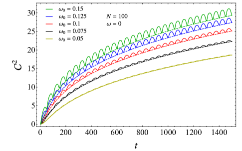
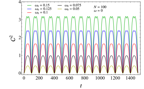
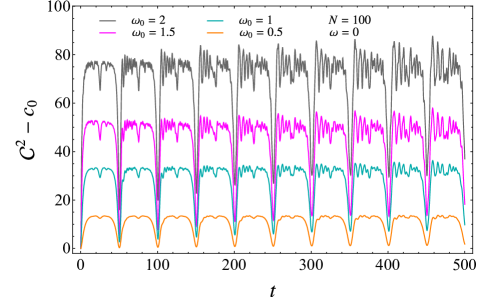
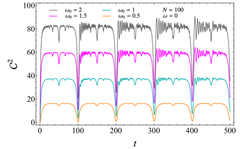
Figure 1: Temporal evolution of the complexity after the global quench w.r.t. the initial state at $t=0$ for harmonic chains with either PBC (left panels) or DBC (right panels) made by $N=100$ sites. The solid lines correspond to the complexity (3.15). In the top left panel, the dashed lines show the zero mode term $c_{0}$ (i.e. the expression multiplyed by $\eta$ in (3.15), which has been subtracted to obtain the bottom left panel), with the same colour code for the corresponding value of $\omega_{0}$.

In Fig. 1 we show the temporal evolution of the complexity (3.15) for various $\omega_{0}$’s, when either PBC (left panels) or DBC (right panels) are imposed. Since $N$ is finite, the revivals already studied in the temporal evolutions of other quantities [97] are observed also in the temporal evolution of the complexity, with a period given by $N/2$ for PBC and by $N$ for DBC. The most important qualitative difference between PBC and DBC is the overall growth observed for PBC, which does not occur for DBC. This growth is due to the zero mode contribution occurring in the complexity (3.15) for PBC. Indeed, when the corresponding term is subtracted, as done in the bottom left panel of Fig. 1, the resulting curve is similar to the temporal evolution of the complexity when DBC hold.

Finally, let us remark that the effect of the decoherence as $t$ increases is more evident for higher values of $\omega_{0}$. For PBC this is observed once the zero mode contribution has been subtracted (see the bottom left panel of Fig. 1).

In [18] the temporal evolution of the complexity of a thermofield double state is considered by taking the unentangled product state as the reference state (in this setup, the choice $\omega=0$ is not allowed). Despite this temporal evolution is different from the one investigated in this manuscript, it also exhibits an overall logarithmic growth due to the zero mode contribution.

3.3 Bounds

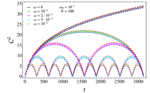
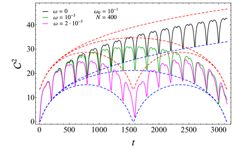
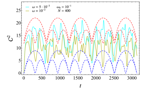
Figure 2: Temporal evolution of the complexity (3.7) (solid lines) and of the corresponding bounds in (2.40) for PBC. The blue and red dashed lines show the lower and the upper bounds, from (2.34) and (2.39) respectively.

It is instructive to discuss further the bounds for the complexity introduced in Sec. 2.3.1 in the special cases of the harmonic chains with either PBC or DBC.

In Fig. 2 we show the complexity (3.7) and the corresponding bounds (2.40) for harmonic chains with PBC. In this case the zero mode term influences the bounds in a crucial way. In Fig. 2, the bounds (2.40) correspond to the red and blue dashed lines, while in the top left panel of Fig. 1, where $\omega=0$, the lower bound in (2.40) is shown through the dashed curves.

In the temporal evolutions of the complexity for PBC displayed in the top panel of Fig. 2, we can identify two periods approximatively given by $\pi/\omega$ and $N/2$. Considering also the bottom panels of Fig. 2, the revivals observed for the critical evolution in Fig. 1 for PBC and $\omega=0$ occur also when $\omega>0$ whenever $\frac{\pi}{\omega}\gg\frac{N}{2}$. The bottom panels in Fig. 2 highlight that the revivals are not observed when $\omega$ is large enough with respect to $1/N$.

For PBC, by comparing the top panel with the bottom ones in Fig. 2, which differ for the size $N$ of the chain, we notice that the bounds (2.40) are very efficient when $\frac{\pi}{\omega}\gg\frac{N}{2}$, while they become not useful away from this regime. In our numerical investigations we have also observed that the bounds (2.40) are not useful when $\omega>\omega_{0}$.

When DBC hold, the lower bound in (2.40) is trivial and the upper bound is a constant.

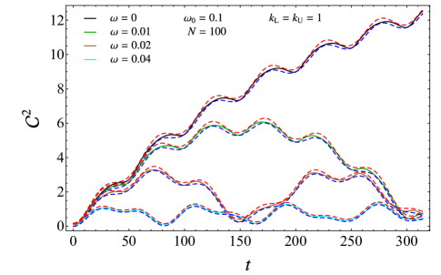
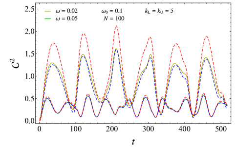
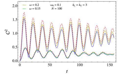
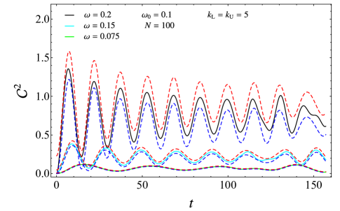
Figure 3: Temporal evolution of the complexity (3.7) (solid lines) and of the corresponding bounds in (3.16) for harmonic chains with either PBC (left panels) or DBC (right panels) and $N=100$. The blue (red) dashed lines correspond to the lower (upper) bound (see (3.18) and (3.17) for the left panels and (3.19) for the right panels). In all the panels $\omega_{0}=0.1$.

The bounds (2.46) can be written explicitly for the harmonic chains that we are considering by setting either $\eta=1$ or $\eta=0$ and employing either (3.4) or (3.6) for the dispersion relations when either PBC or DBC respectively are imposed. The resulting expressions for these bounds require to sum either $N$ or $N-1$ terms and we can obtain less constraining but still insightful bounds by keeping only few terms in these sums, i.e.

$$\mathcal{C}^{2}_{\textrm{\tiny L},k_{\textrm{\tiny L}}}\,\leqslant\,\mathcal{C}^{2}\,\leqslant\,\mathcal{C}^{2}_{\textrm{\tiny U},k_{\textrm{\tiny U}}}$$ (3.16)

where $k_{\textrm{\tiny L}}$ and $k_{\textrm{\tiny U}}$ are independent parameters related to the number of terms in the sum kept to define the corresponding bound. Since the explicit expressions of the dispersion relations are important to write explicitly the bounds in (3.16), the cases of PBC and DBC must be studied separately.

Considering PBC first, one observes that the corresponding $f_{\textrm{\tiny L}}(\tilde{x}_{k})$ as function of $k$ (that can be constructed from (2.48), (2.43) and (3.4)) is large when $k\simeq 1$ and $k\simeq N-1$, while it becomes negligible in the middle of the interval $[1,N-1]$. This leads to sum just over $k=1,\dots,k_{\textrm{\tiny L}}$ and $k=N-k_{\textrm{\tiny L}},\dots,N-1$, for some $k_{\textrm{\tiny L}}$. Thus, by employing also the symmetry $k\leftrightarrow N-k$ of the dispersion relations (3.4), the lower bound in (3.16) for PBC reads

$$\mathcal{C}^{2}_{\textrm{\tiny L},k_{\textrm{\tiny L}}}=c_{0}+2\sum_{k=1}^{k_{\textrm{\tiny L}}}f_{\textrm{\tiny L}}(\tilde{x}_{k})\,[\sin(\Omega_{k}t)]^{2}\,.$$ (3.17)

The upper bound $\mathcal{C}^{2}_{\textrm{\tiny U},k_{\textrm{\tiny U}}}$ can be found through similar considerations applied to the function $f_{\textrm{\tiny U}}(\tilde{x}_{k})$ introduced in (2.48). This leads to sum the terms whose $k$ is close to the boundary of $[1,N-1]$ keeping their dependence on $t$ and to set $\sin^{2}(\Omega_{k}t)=1$ in the remaining ones, which must not be discarded. The resulting bound is

$$\mathcal{C}^{2}_{\textrm{\tiny U},k_{\textrm{\tiny U}}}\,=\,c_{0}+2\sum_{k=1}^{k_{\textrm{\tiny U}}}f_{\textrm{\tiny U}}(\tilde{x}_{k})\,[\sin(\Omega_{k}t)]^{2}+\!\!\sum_{k=k_{\textrm{\tiny U}}+1}^{\lfloor\frac{N-1}{2}\rfloor}\!\!2\,f_{\textrm{\tiny U}}(\tilde{x}_{k})+f_{\textrm{\tiny U}}(\tilde{x}_{N/2})\,\big{|}\cos(\pi N/2)\big{|}\,.$$ (3.18)

The bounds (2.46) are recovered when $k_{\textrm{\tiny L}}=k_{\textrm{\tiny U}}=\lfloor\frac{N-1}{2}\rfloor$, by setting to zero the second sum in the r.h.s. of (3.18) and by restoring the time dependence in the term having $k=N/2$ when $N$ is even, both in (3.17) and (3.18).

When DBC are imposed, a similar analysis can be carried out, with the crucial difference that the symmetry $k\leftrightarrow N-k$ in the dispersion relations (3.6) does not occur in this case. Setting $\eta=0$ and employing the dispersion relations (3.6), one obtains (3.16) with

$$\mathcal{C}^{2}_{\textrm{\tiny L},k_{\textrm{\tiny L}}}\equiv\sum_{k=1}^{k_{\textrm{\tiny L}}}f_{\textrm{\tiny L}}(\tilde{x}_{k})\,[\sin(\Omega_{k}t)]^{2}\;\;\qquad\;\;\mathcal{C}^{2}_{\textrm{\tiny U},k_{\textrm{\tiny U}}}\equiv\sum_{k=1}^{k_{\textrm{\tiny U}}}f_{\textrm{\tiny U}}(\tilde{x}_{k})\,[\sin(\Omega_{k}t)]^{2}+\!\!\sum_{k=k_{\textrm{\tiny U}}+1}^{N-1}\!\!f_{\textrm{\tiny U}}(\tilde{x}_{k})$$ (3.19)

where $1\leqslant k_{\textrm{\tiny L}},k_{\textrm{\tiny U}}\leqslant N-1$. In order to recover (2.46) from (3.16), we have to choose $k_{\textrm{\tiny L}}=k_{\textrm{\tiny U}}=N-1$ and set to zero the last sum in the second expression of (3.19).

By construction, we have $\mathcal{C}^{2}_{\textrm{\tiny L},k_{\textrm{\tiny L}}}\leqslant\mathcal{C}^{2}_{\textrm{\tiny L}}$ and $\mathcal{C}^{2}_{\textrm{\tiny U},k_{\textrm{\tiny U}}}\geqslant\mathcal{C}^{2}_{\textrm{\tiny U}}$, but $\mathcal{C}^{2}_{\textrm{\tiny L},k_{\textrm{\tiny L}}}$ and $\mathcal{C}^{2}_{\textrm{\tiny U},k_{\textrm{\tiny U}}}$ contain less terms than $\mathcal{C}^{2}_{\textrm{\tiny L}}$ and $\mathcal{C}^{2}_{\textrm{\tiny U}}$ respectively, hence they are easier to evaluate and to study analytically. For both PBC and DBC, considering either the lower or the upper bound in (3.16), it improves as either $k_{\textrm{\tiny L}}$ or $k_{\textrm{\tiny U}}$ respectively increases.

In Fig. 3 we show the bounds (3.16) when either PBC (left panels) or DBC (right panels) are imposed and small values of $k_{\textrm{\tiny L}}$ and $k_{\textrm{\tiny U}}$ are considered. For given values of $k_{\textrm{\tiny L}}$ and $k_{\textrm{\tiny U}}$, the agreement between the bounds and the exact curve improves as $|\omega_{0}-\omega|$ decreases. Notice that higher values of $k_{\textrm{\tiny L}}$ and $k_{\textrm{\tiny U}}$ are needed for DBC to reach an agreement with the exact curve comparable with the one obtained for PBC.

3.4 Large $N$

It is important to study approximate expressions for the temporal evolution of the complexity when large values of $N$ are considered.

In our numerical analysis, we noticed that, for finite but large enough values of $N\gtrsim 10$ the complexity (3.7) is well described by a function of $\omega N$, $\omega_{0}N$ and $t/N$. This function, which depends on whether PBC or DBC are imposed, can be written by introducing the approximation $\sin(x)\simeq x$ into the dispersion relations and keeping only the leading term (see appendix C.1 for a more detailed discussion). For PBC we find

$$\mathcal{C}_{\textrm{\tiny approx}}\,=\,\sqrt{c_{0}(t)+2\!\!\sum_{k=1}^{\lfloor\frac{N-1}{2}\rfloor}\!\left[\textrm{arcsinh}\!\left(\,\frac{(\omega N)^{2}-(\omega_{0}N)^{2}}{2\,\widetilde{\Omega}^{\textrm{\tiny(P)}}_{k}\,\widetilde{\Omega}^{\textrm{\tiny(P)}}_{0,k}}\,\sin\!\big{(}\widetilde{\Omega}^{\textrm{\tiny(P)}}_{k}t/N\big{)}\right)\right]^{2}}$$ (3.20)

where $c_{0}(t)$ is (3.8); while for DBC we get

$$\mathcal{C}_{\textrm{\tiny approx}}=\sqrt{\,\sum_{k=1}^{N-1}\left[\textrm{arcsinh}\!\left(\,\frac{(\omega N)^{2}-(\omega_{0}N)^{2}}{2\,\widetilde{\Omega}^{\textrm{\tiny(D)}}_{k}\widetilde{\Omega}^{\textrm{\tiny(D)}}_{0,k}}\,\sin\!\big{(}\widetilde{\Omega}^{\textrm{\tiny(D)}}_{k}t/N\big{)}\right)\right]^{2}}$$ (3.21)

where

$$\widetilde{\Omega}^{\textrm{\tiny(P)}}_{k}=\sqrt{(\omega N)^{2}+\frac{4\pi^{2}\kappa}{m}\,k^{2}}\,\,\qquad\,\,\widetilde{\Omega}^{\textrm{\tiny(D)}}_{k}=\sqrt{(\omega N)^{2}+\frac{\pi^{2}\kappa}{m}\,k^{2}}$$ (3.22)

while $\widetilde{\Omega}^{\textrm{\tiny(P)}}_{0,k}$ and $\widetilde{\Omega}^{\textrm{\tiny(D)}}_{0,k}$ are obtained by replacing $\omega$ with $\omega_{0}$ in these expressions. Notice that both (3.20) and (3.21) depend on $\omega N$, $\omega_{0}N$ and $t/N$. These approximate expressions have been used to plot the dashed light grey curves in the top panels of Fig. 4, which nicely agree with the corresponding solid coloured curves.

The thermodynamic limit $N\to\infty$ of the complexity can be studied through the standard procedure. Introducing $\theta\equiv\pi k/N$ and substituting $\sum_{k}\to\frac{N}{\pi}\int_{0}^{\pi}d\theta$ in (3.7), at the leading order we find

$$\mathcal{C}_{\textrm{\tiny TD}}=\sqrt{\frac{N}{\pi}}\;\sqrt{\int_{0}^{\pi}\left[\textrm{arcsinh}\!\left(\,\frac{\omega^{2}-\omega_{0}^{2}}{2\,\Omega_{\theta}\,\Omega_{0,\theta}}\,\sin(\Omega_{\theta}\,t)\right)\right]^{2}\!d\theta}$$ (3.23)

where the dispersion relations for PBC and DBC become respectively

$$\Omega_{0,\theta}=\sqrt{\omega_{0}^{2}+\frac{4\kappa}{m}\,(\sin\theta)^{2}}\,\,\qquad\,\,\Omega_{\theta}=\sqrt{\omega^{2}+\frac{4\kappa}{m}\,(\sin\theta)^{2}}$$ (3.24)

and

$$\Omega_{0,\theta}=\sqrt{\omega_{0}^{2}+\frac{4\kappa}{m}\,[\sin(\theta/2)]^{2}}\,\,\qquad\,\,\Omega_{\theta}=\sqrt{\omega^{2}+\frac{4\kappa}{m}\,[\sin(\theta/2)]^{2}}\;.$$ (3.25)

Notice that, for PBC, the zero mode does not contribute because $c_{0}/N\to 0$ as $N\to\infty$. When DBC hold, by using the dispersion relations (3.25), changing of variable $\tilde{\theta}=\theta/2$ in (3.23) and exploiting the symmetry of the function $\sin(x)$ in the interval $[0,\pi]$, one finds that (3.23) with (3.24) holds for both PBC and DBC. Thus, the leading order of this limit is independent of the boundary conditions. This means that the complexity does not distinguish the boundary conditions in this regime. Indeed, in the left and right panels of Fig. 4, the same function (just described) has been used to plot the dashed black curves.

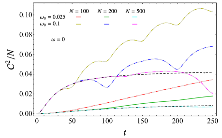
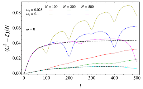
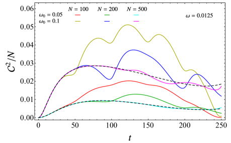
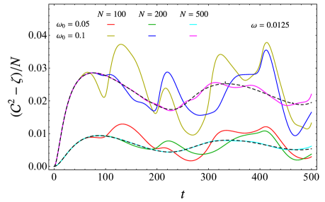
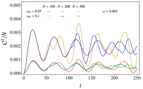
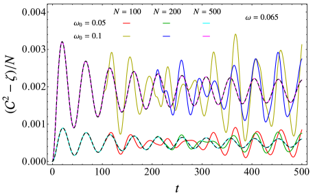
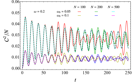
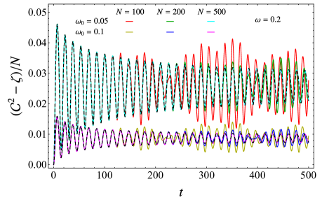
Figure 4: Temporal evolutions of the complexity for harmonic chains with either PBC (left panels) or DBC (right panels). The solid lines show $\mathcal{C}^{2}/N$ for PBC and $(\mathcal{C}^{2}-\zeta)/N$ for DBC, with $\mathcal{C}$ given by (3.7) and $\zeta$ by (C.2). The dashed black lines represent $\mathcal{C}_{\textrm{\tiny TD}}^{2}/N$, from (3.23).

The boundary conditions become crucial in the subleading term of the expansion of (3.7) as $N\to\infty$, which can be studied through the Euler-Maclaurin formula [98]. The details of this analysis are discussed in appendix C.2 and the final result is

$$\mathcal{C}^{2}-\mathcal{C}_{\textrm{\tiny TD}}^{2}=R_{1,\infty}^{\textrm{\tiny(B)}}\;\;\qquad\;\;\textrm{B}\in\big{\{}\textrm{P},\textrm{D}\big{\}}\;\;\qquad\;\;R_{1,\infty}^{\textrm{\tiny(B)}}=\left\{\begin{array}[]{ll}R_{1,\infty}^{\textrm{\tiny(P)}}&\textrm{PBC}\\ \rule{0.0pt}{19.91684pt}\displaystyle R_{1,\infty}^{\textrm{\tiny(D)}}=\frac{R_{1,\infty}^{\textrm{\tiny(P)}}}{2}+\zeta&\textrm{DBC}\end{array}\right.$$ (3.26)

where $R_{1,\infty}^{\textrm{\tiny(P)}}$ and $\zeta$ are the time-dependent functions given in (C.17) and in (C.2) respectively. Numerical checks for these results are shown in Fig. 4. In the top panels of this figure we have displayed also $\mathcal{C}_{\textrm{\tiny approx}}/N$ from (3.20) (left panel) and $(\mathcal{C}_{\textrm{\tiny approx}}-\zeta)/N$ from (3.21) (right panel) through dashed light grey lines.

In the continuum limit, $N\to\infty$ and the lattice spacing $a\equiv\sqrt{m/\kappa}\to 0$ is vanishing while $Na\equiv\ell$ is kept fixed. In this limit, the expression (3.7) for the complexity (which holds for both PBC and DBC) becomes

$$\mathcal{C}_{\textrm{\tiny cont}}=\sqrt{\frac{\ell}{2\pi}}\,\sqrt{\int_{-\infty}^{\infty}\left[\textrm{arcsinh}\!\left(\,\frac{\omega^{2}-\omega_{0}^{2}}{2\,\Omega_{p}\,\Omega_{0,p}}\,\sin(\Omega_{p}t)\right)\right]^{2}\!dp}$$ (3.27)

(see appendix C.3 for a detailed discussion) where

$$\Omega_{0,p}=\sqrt{\omega_{0}^{2}+p^{2}}\,\,\qquad\,\,\Omega_{p}=\sqrt{\omega^{2}+p^{2}}\,.$$ (3.28)

Since $\Omega_{p}\simeq p$ when $p\gg\omega$, the vanishing of the integrand in (3.27) as $p\to\pm\infty$ is such that the complexity is UV finite. We remark that, instead, when the reference state is the unentangled product state, the continuum limit of the complexity is UV divergent, as discussed in appendix C.3; hence a UV cutoff in the integration domain over $p$ must be introduced.

3.5 Initial growth

It is worth discussing the initial growth of the complexity for the harmonic chains that we are considering. Since the complexity (3.7) is a special case of (2.33), its expansion as $t\to 0$ can be found by specialising the expansion (2.36) and its coefficients (2.37) and (2.38) to the harmonic chains with either PBC or DBC. For the sake of simplicity, in the following we discuss only the leading term (i.e. only the coefficient $b_{1}$ in (2.37)), which provides the linear growth, but a similar analysis can be applied straightforwardly to the coefficients of the higher order terms in the $t\to 0$ expansion.

For the harmonic chains with either PBC or DBC, the linear growth in (2.36) becomes

$$\mathcal{C}\,=\,\frac{|\omega^{2}-\omega^{2}_{0}|}{2}\,\Bigg{(}\sum_{k=1}^{N-1+\eta}\!\Omega_{0,k}^{-2}\Bigg{)}^{1/2}t\,+O(t^{3})$$ (3.29)

where $\eta=1$ and (3.4) must be used for PBC, while $\eta=0$ and (3.6) must be employed for DBC. We remark that the slope of the initial linear growth in (3.29) is proportional to $|\omega-\omega_{0}|$.

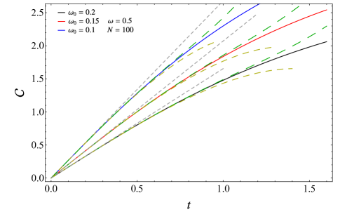
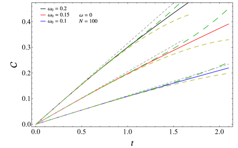
Figure 5: Initial growth of the complexity for harmonic chains with PBC and $N=100$. The evolution Hamiltonian is either massive (left panel) or massless (right panel), for three values $\omega_{0}$. The solid lines show the complexity (3.7) (with (3.4)) and the dashed lines represent its expansion (2.36) up to the $O(t)$ (grey), $O(t^{3})$ (yellow) and $O(t^{5})$ (green) term included.

In Fig. 5, we consider the initial growth of the complexity (3.7) when PBC are imposed, comparing the exact curve against its expansion (2.36). The corresponding analysis for DBC provides curves that are very similar to the ones displayed in Fig. 5; hence it has not been reported in this manuscript.

Let us conclude our discussion about the temporal evolution of the complexity of pure states with a brief qualitative comparison between the results discussed above and the corresponding ones for the temporal evolution of the holographic complexity [10, 8, 13, 14, 9, 51, 52, 53].

The Vaidya spacetimes are the typical backgrounds employed as the gravitational duals of global quantum quenches in the conformal field theory on their boundary. They describe the formation of a black hole through the collapse of a matter shell. In Vaidya spacetimes, the temporal evolution of the holographic entanglement entropy has been largely studied [64, 65, 99, 100, 101, 102, 103, 104] and the temporal evolutions of the holographic complexity for the entire spatial section of the conformal field theory on the boundary has been investigated in [51, 52, 53, 105]. Considering the temporal evolution of the rate $\frac{d\mathcal{C}}{dt}$ allows to avoid the problem of choosing the reference state, which deserves further clarifications for the holographic complexity, even for static gravitational backgrounds. The analysis of $\frac{d\mathcal{C}}{dt}$ in Vaidya spacetimes, both for the CV and for the CA prescriptions, shows that these temporal evolutions are linear in time both at very early and at late time [51, 52]. While also the initial growth of the complexity that we have explored is linear (see (3.29)), the late time growth is at most logarithmic. This disagreement, which deserves further analysis, has been discussed in [18].

We find it worth observing also that the coefficient of the initial growth (3.29) is proportional to $|\omega^{2}-\omega_{0}^{2}|$ and that the corresponding coefficient for the holographic complexity is proportional to the mass of the final black hole [52, 51].

4 Subsystem complexity in finite harmonic chains

In this section we study the temporal evolution of the subsystem complexity after a global quench. The reference and the target states are the reduced density matrices associated to a given subsystem. We focus on the simple cases where the subsystem $A$ is a block made by consecutive sites in harmonic chains with either PBC or DBC.

4.1 Subsystem complexity

In the harmonic lattices that we are considering, the reduced density matrix associated to $A$ characterises a Gaussian state which can be described equivalently through its reduced covariance matrix $\gamma_{A}$. This matrix is constructed by considering the reduced correlation matrices $Q_{A}$, $P_{A}$ and $M_{A}$, whose elements are respectively given by $(Q_{A})_{i,j}=\langle\psi_{0}|\,\hat{q}_{i}(t)\,\hat{q}_{j}(t)\,|\psi_{0}\rangle$, $(P_{A})_{i,j}=\langle\psi_{0}|\,\hat{p}_{i}(t)\,\hat{p}_{j}(t)\,|\psi_{0}\rangle$ and $(M_{A})_{i,j}=\textrm{Re}\big{[}\langle\psi_{0}|\,\hat{q}_{i}(t)\,\hat{p}_{j}(t)\,|\psi_{0}\rangle\big{]}$ with $i,j\in A$, which depend also on the time after the global quench. These matrices provide the following block decomposition of the reduced covariance matrix

$$\gamma_{A}(t)=\,\bigg{(}\begin{array}[]{cc}Q_{A}(t)&M_{A}(t)\\ M_{A}(t)^{\textrm{t}}&P_{A}(t)\\ \end{array}\bigg{)}\,.$$ (4.1)

For the harmonic chains with either PBC or DBC introduced in Sec. 3 and $A$ made by $L$ consecutive sites, $Q_{A}$ and $P_{A}$ are $L\times L$ symmetric matrices and $\gamma_{A}$ is a real, symmetric and positive definite $2L\times 2L$ matrix.

Adapting the analysis made in Sec. 3 for pure states to the mixed states described by the reduced covariance matrices $\gamma_{A}(t)$, we have that the reference state is given by the reduced density matrix for the interval $A$ at time $t_{\textrm{\tiny R}}\geqslant 0$ obtained through the quench protocol characterised by $\big{(}\kappa_{\textrm{\tiny R}},m_{\textrm{\tiny R}},\omega_{\textrm{\tiny R}},\omega_{0,\textrm{\tiny R}}\big{)}$ and the target state by the reduced density matrix for the same interval at time $t_{\textrm{\tiny T}}\geqslant t_{\textrm{\tiny R}}$ constructed through the quench protocol described by $\big{(}\kappa_{\textrm{\tiny T}},m_{\textrm{\tiny T}},\omega_{\textrm{\tiny T}},\omega_{0,\textrm{\tiny T}}\big{)}$. The corresponding reduced covariance matrices are denoted by $\gamma_{\textrm{\tiny R},A}(t_{\textrm{\tiny R}})$ and $\gamma_{\textrm{\tiny T},A}(t_{\textrm{\tiny T}})$ respectively. These reduced covariance matrices are decomposed in terms of the correlation matrices of the subsystem like in (4.1).

The approach to the circuit complexity of mixed states based on the Fisher information geometry [74] allows to construct the optimal circuit between $\gamma_{\textrm{\tiny R},A}(t_{\textrm{\tiny R}})$ and $\gamma_{\textrm{\tiny T},A}(t_{\textrm{\tiny T}})$. The covariance matrices along this optimal circuit are

$$G_{s}(\gamma_{\textrm{\tiny R},A}(t_{\textrm{\tiny R}})\,,\gamma_{\textrm{\tiny T},A}(t_{\textrm{\tiny T}}))\,\equiv\,\gamma_{\textrm{\tiny R},A}(t_{\textrm{\tiny R}})^{1/2}\Big{(}\gamma_{\textrm{\tiny R},A}(t_{\textrm{\tiny R}})^{-1/2}\,\gamma_{\textrm{\tiny T},A}(t_{\textrm{\tiny T}})\,\gamma_{\textrm{\tiny R},A}(t_{\textrm{\tiny R}})^{-1/2}\Big{)}^{s}\gamma_{\textrm{\tiny R},A}(t_{\textrm{\tiny R}})^{1/2}$$ (4.2)

where $0\leqslant s\leqslant 1$ parameterises the optimal circuit. The length of this optimal circuit is proportional to its complexity

$$\mathcal{C}_{A}\,=\,\frac{1}{2\sqrt{2}}\;\sqrt{\,\textrm{Tr}\,\Big{\{}\big{[}\log\!\big{(}\gamma_{\textrm{\tiny T},A}(t_{\textrm{\tiny T}})\,\gamma_{\textrm{\tiny R},A}(t_{\textrm{\tiny R}})^{-1}\big{)}\big{]}^{2}\Big{\}}}\;.$$ (4.3)

Considering harmonic chains made by $N$ sites where PBC are imposed, by using (2.5), (2.6) and either (3.2) or (3.3), one obtains the elements of the correlation matrices whose reduction to $A$ provides (4.1). They read

$$Q_{i,j}(t) = \frac{1}{N}\sum_{k=1}^{N}Q_{k}(t)\,\cos\!\big{[}(i-j)\,2\pi k/N\big{]}$$

$$\rule{0.0pt}{22.76228pt}P_{i,j}(t) = \frac{1}{N}\sum_{k=1}^{N}P_{k}(t)\,\cos\!\big{[}(i-j)\,2\pi k/N\big{]}$$ (4.4)

$$\rule{0.0pt}{22.76228pt}M_{i,j}(t) = \frac{1}{N}\,\sum_{k=1}^{N}M_{k}(t)\,\cos\!\big{[}(i-j)\,2\pi k/N\big{]}$$

where $1\leqslant i,j\leqslant N$; while for DBC, by using (3.5), one obtains the following correlators

$$Q_{i,j}(t) = \frac{2}{N}\sum_{k=1}^{N}Q_{k}(t)\,\sin\!\big{(}i\,\pi k/N\big{)}\,\sin\!\big{(}j\,\pi k/N\big{)}$$

$$\rule{0.0pt}{22.76228pt}P_{i,j}(t) = \frac{2}{N}\sum_{k=1}^{N}P_{k}(t)\,\sin\!\big{(}i\,\pi k/N\big{)}\,\sin\!\big{(}j\,\pi k/N\big{)}$$ (4.5)

$$\rule{0.0pt}{22.76228pt}M_{i,j}(t) = \frac{2}{N}\,\sum_{k=1}^{N}M_{k}(t)\,\sin\!\big{(}i\,\pi k/N\big{)}\,\sin\!\big{(}j\,\pi k/N\big{)}$$

where $1\leqslant i,j\leqslant N-1$. In these correlators, the functions $Q_{k}(t)$, $P_{k}(t)$ and $M_{k}(t)$ are given by (2.6), with either (3.4) for PBC or (3.6) for DBC.

The reduced covariance matrices $\gamma_{\textrm{\tiny R},A}(t_{\textrm{\tiny R}})$ and $\gamma_{\textrm{\tiny T},A}(t_{\textrm{\tiny T}})$ for the block $A$ providing the optimal circuit (4.2) and its complexity (4.3) are constructed as in (4.1), through the reduced correlation matrices $Q_{A}$, $P_{A}$ and $M_{A}$, obtained by restricting to $i,j\in A$ the indices of the correlation matrices whose elements are given in (4.1) and (4.1).

We remark that the matrix $\widetilde{V}$ in (2.5) (given in (3.2) or (3.3) for PBC and in (3.5) for DBC) is crucial to write (4.1) and (4.1); hence it enters in a highly non-trivial way in the evaluation of the subsystem complexity. Instead, it does not affect the complexity for the entire system, where both the reference and the target states are pure states, as remarked below (2.20).

4.2 Numerical results

Considering the global quench that we are exploring, in the following we discuss some numerical results for the temporal evolution of the subsystem complexity of a block $A$ made by $L$ consecutive sites in harmonic chains made by $N$ sites, where either PBC or DBC are imposed. We focus on the simplest setup where the reference state is the initial state (hence $t_{\textrm{\tiny R}}=0$) and the target state corresponds to a generic value of $t_{\textrm{\tiny T}}=t\geqslant 0$ after the quench. The remaining parameters are fixed to $\omega_{0,\textrm{\tiny R}}=\omega_{0,\textrm{\tiny T}}\equiv\omega_{0}$, $\omega_{\textrm{\tiny R}}=\omega_{\textrm{\tiny T}}\equiv\omega$, $\kappa_{\textrm{\tiny R}}=\kappa_{\textrm{\tiny T}}=1$ and $m_{\textrm{\tiny R}}=m_{\textrm{\tiny T}}=1$. In the case of DBC, we consider both $A$ adjacent to the boundary and separated from it.

In this setup, the subsystem complexity (4.3) can be written as

$$\mathcal{C}_{A}\,=\,\frac{1}{2\sqrt{2}}\;\sqrt{\,\textrm{Tr}\,\Big{\{}\big{[}\log\!\big{(}\gamma_{A}(t)\,\gamma_{A}(0)^{-1}\big{)}\big{]}^{2}\Big{\}}}\;.$$ (4.6)

It is natural to introduce also the entanglement entropy $S_{A}(t)$ and its initial value $S_{A}(0)$, which lead to define the increment of the entanglement entropy w.r.t. its initial value, i.e.

$$\Delta S_{A}\equiv S_{A}(t)-S_{A}(0)$$ (4.7)

where $S_{A}(t)$ and $S_{A}(0)$ can be evaluated from the symplectic spectrum of $\gamma_{A}(t)$ and of $\gamma_{A}(0)$ respectively in the standard way [57, 54, 92, 106, 107, 108, 109, 110, 62, 111].

In all the figures discussed in this section we show the temporal evolutions of the subsystem complexity $\mathcal{C}_{A}$ in (4.6) or of the increment $\Delta S_{A}$ of the entanglement entropy in (4.7) after the global quench. In particular, we show numerical results corresponding to $N=100$ and $N=200$, finding nice collapses of the data when $L/N$, $\omega_{0}N$ and $\omega N$ are kept fixed, independently of the boundary conditions. The data reported in all the left panels have been obtained in harmonic chains with PBC, whose dispersion relations are (3.4), while the ones in all the right panels correspond to a block adjacent to a boundary of harmonic chains where DBC are imposed, whose dispersion relations are (3.6), if not otherwise indicated (like in Fig.12). The evolution Hamiltonian is gapless in Fig. 6, Fig. 7, Fig. 8 and Fig. 12, while it is gapped in Fig. 9 and Fig. 10, with $\omega N=5$. In Fig. 11, where the initial growth is explored, both gapless and gapped evolution Hamiltonians have been employed. When $L=N$, the complexity (3.7) for pure states has been evaluated with either $N=100$ (black solid lines) or $N=200$ (dashed green lines).

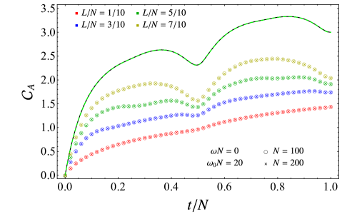
Figure 6: Temporal evolution of $\mathcal{C}_{A}$ in (4.6) after the global quench with gapless evolution Hamiltonian and $\omega_{0}N=20$, for a block $A$ made by $L$ consecutive sites in harmonic chains with either PBC (left panels) or DBC (right panels) made by $N$ sites (in the latter case $A$ is adjacent to a boundary). When $L=N$, the complexity (3.7) is shown for $N=100$ (solid black lines) and $N=200$ (dashed green lines).

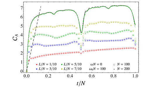
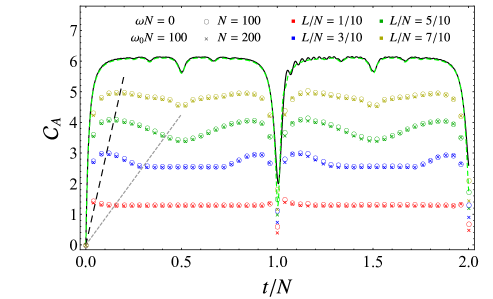
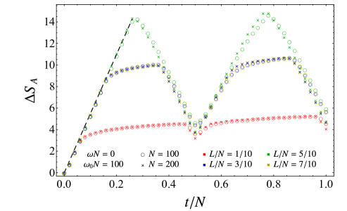
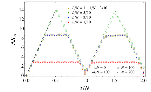
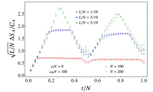
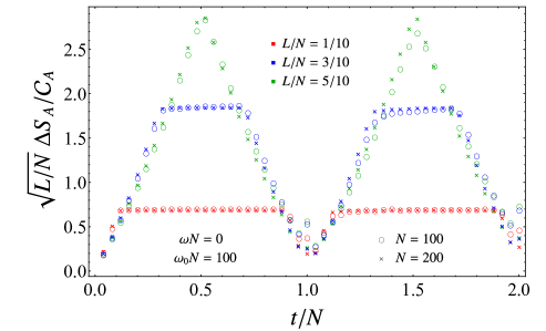
Figure 7: Temporal evolution of $\mathcal{C}_{A}$ in (4.6) (top panels), of $\Delta S_{A}$ in (4.7) (middle panels) and of $\sqrt{L/N}\,\Delta S_{A}/\mathcal{C}_{A}$ (bottom panels) after the global quench with gapless evolution Hamiltonian and $\omega_{0}N=100$, for a block $A$ made by $L$ consecutive sites in a harmonic chains with either PBC (left panels) or DBC (right panels) made by $N$ sites (in the latter case $A$ is adjacent to a boundary). When $L=N$ the complexity (3.7) is shown for $N=100$ (solid black lines) and $N=200$ (dashed green lines).

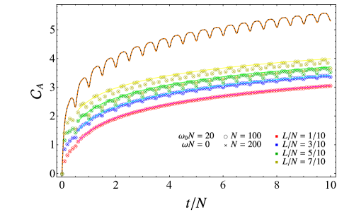
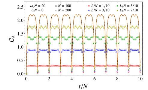
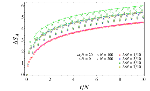
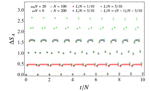
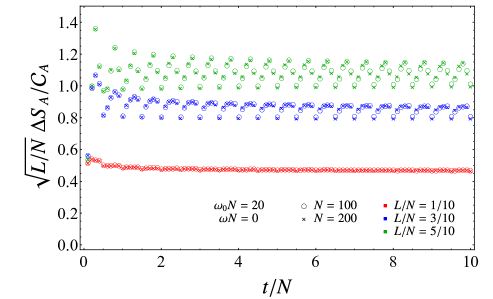
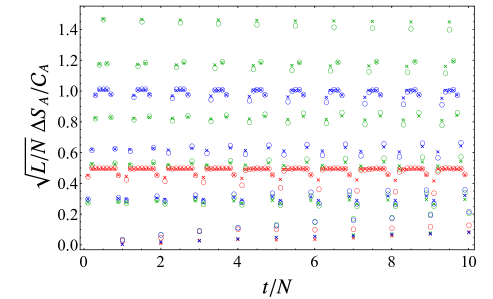
Figure 8: Temporal evolution of $\mathcal{C}_{A}$ in (4.6) (top panels), of $\Delta S_{A}$ in (4.7) (middle panels) and of $\sqrt{L/N}\,\Delta S_{A}/\mathcal{C}_{A}$ (bottom panels) after the global quench with a gapless evolution Hamiltonian and $\omega_{0}N=20$, for harmonic chains with either PBC (left panels) or DBC (right panels), in the same setups of Fig. 6 are considered.

In Fig. 6, Fig. 7 and Fig. 8 all the data have been obtained with $\omega N=0$ and either $\omega_{0}N=20$ (Fig. 6 and Fig. 8) or $\omega_{0}N=100$ (Fig. 7). Revivals are observed and the different cycles correspond to $p<2t/N<p+1$ for PBC and to $p<t/N<p+1$ for DBC, where $p$ is a non-negative integer.

The qualitative behaviour of the temporal evolution of the subsystem complexity crucially depends on the boundary conditions of the harmonic chain. For DBC, considering the data having $L/N<1/2$ when $t/N<1/2$, we can identify three regimes: an initial growth until a local maximum is reached, a decrease and then a thermalisation regime after certain value of $t/N$, where the subsystem complexity remains constant. For PBC and $L/N<1/2$, the latter regime is not observed and $\mathcal{C}_{A}$ keeps growing. Comparing the right panel in Fig. 6 with the top right panel in Fig. 7, one realises that, for DBC, the height of the plateaux increases as either $L/N$ or $\omega_{0}N$ increases, as expected. The absence of thermalisation regimes for PBC could be related to the occurrence of the zero mode, as suggested by the fact that, for pure states, the zero mode contribution provides the logarithmic growth of the complexity (3.15). However, we are not able to identify explicitly the zero mode contribution in the subsystem complexity, hence we cannot subtract it as done in the bottom left panel of Fig. 1 for the temporal evolution of the complexity of pure states.

For DBC, the plateau in the thermalisation regime is not observed when $L/N\geqslant 1/2$ and, considering the interval $t/N\in[\nu,\nu+1]$ with $\nu=\{0,1\}$, it approximately begins at $t-\nu N\simeq L$ and ends at $t-\nu N\simeq N-L+1$. The straight dashed grey lines approximatively indicate the beginning of the plateaux for different $L/N<1/2$ (in particular, they are obtained by joining the origin with the point of the curve made by the blue data points at $t/N=0.3$).

We remark that the temporal evolution of $\mathcal{C}_{A}$ in infinite chains is made by the three regimes mentioned above (see Fig. 14, Fig. 15 and Fig. 16), as largely discussed in Sec. 5.

Comparing the temporal evolutions of $\mathcal{C}_{A}$ and $\Delta S_{A}$ for the same quench protocol and the same subsystem in Fig. 7, we observe that the initial growth of $\mathcal{C}_{A}$ in the first revival is faster than the linear initial growth of $\Delta S_{A}$, as highlighted by the straight dashed black lines in Fig. 7. Within the first revival, we do not observe a long range of $t/N$ where the evolution of $\mathcal{C}_{A}$ is linear. Nonetheless, the straight line characterising the initial growth of $\Delta S_{A}$ intersects the first local maximum corresponding to the end of the initial growth of $\mathcal{C}_{A}$ when $L/N<1/2$. Considering the data points for $L/N<1/2$ and the initial regime of $t/N$ corresponding to half of the first revival, we notice that, while the temporal evolution of $\Delta S_{A}$ displays a linear growth followed by a saturation regime, the temporal evolution of $\mathcal{C}_{A}$ is characterised by the three regimes described above. The saturation regimes of $\mathcal{C}_{A}$ and $\Delta S_{A}$ are qualitatively very similar and begin approximatively at the same value of $t/N$. Notice that the amplitude of the decrease of $\mathcal{C}_{A}$ at the end of the first revival is smaller than the one of $\Delta S_{A}$.

The temporal evolutions of $\mathcal{C}_{A}$ and $\Delta S_{A}$ can be compared for $L/N\leqslant 1/2$. Indeed, for a bipartite system in a pure state the entanglement entropy of a subsystem is equal to the entanglement entropy of the complementary subsystem. This property, which does not hold for $\mathcal{C}_{A}$, implies the overlap between the data for $\Delta S_{A}$ corresponding to $L/N=3/10$ and to $L/N=7/10$. Furthermore, $\Delta S_{A}=0$ identically when $L=N$.

In the bottom panels of Fig. 7 we have reported the temporal evolutions of the ratio $\Delta S_{A}/\mathcal{C}_{A}$ for the data reported in the other panels of the figure. The curves of $\Delta S_{A}/\mathcal{C}_{A}$ corresponding to PBC (left panel) and DBC (right panel) are very similar. For instance, the curves for $\sqrt{L/N}\,\Delta S_{A}/\mathcal{C}_{A}$ have the same initial growth for different values of $L/N$. However, we remark that a mild logarithmic decrease occurs in the thermalisation regime for PBC.

In Fig. 8 the range $0\leqslant t/N\leqslant 10$ is considered, which is made by 20 revivals for PBC and by 10 cycles for DBC. The temporal evolutions of $\mathcal{C}_{A}$ in the top panels show that, up to oscillations due to the revivals, after the initial growth $\mathcal{C}_{A}$ keeps growing logarithmically for PBC (the solid coloured lines in the top left panel are two-parameter fits through the function $a+b\log(t/N)$ of the corresponding data), while it remains constant for DBC. This feature is observed also in the corresponding temporal evolutions of $\Delta S_{A}$ (middle panels of Fig. 8). These two logarithmic growths for PBC are very similar, as shown by the temporal evolution of $\Delta S_{A}/\mathcal{C}_{A}$ displayed in the bottom left panel of Fig. 8.

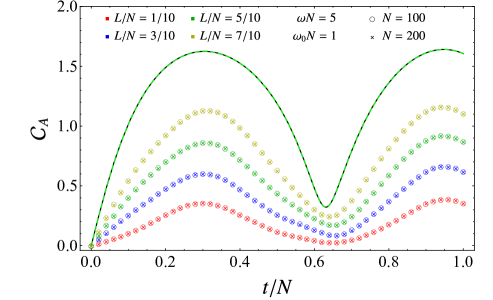
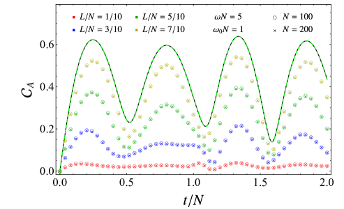
Figure 9: Temporal evolution of $\mathcal{C}_{A}$ in (4.6) after the global quench with a gapped evolution Hamiltonian for a block $A$ made by $L$ consecutive sites in harmonic chains with either PBC (left panels) or DBC (right panels) made by $N$ sites (in the latter case $A$ is adjacent to a boundary of the segment). When $L=N$ the complexity (3.7) is shown for $N=100$ (solid black lines) and $N=200$ (dashed green lines).

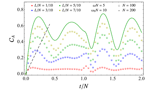
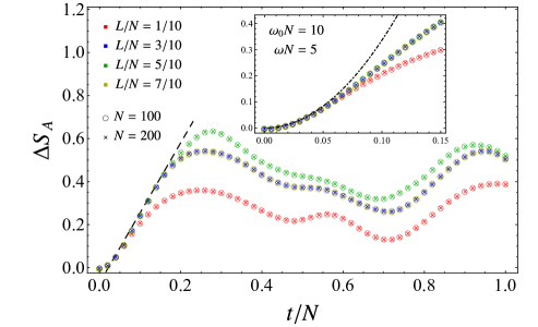
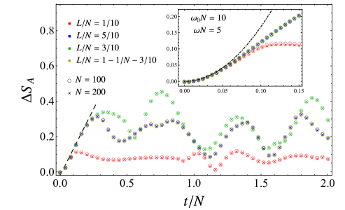
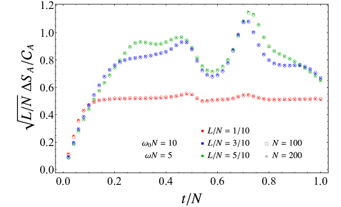
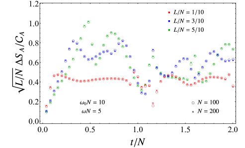
Figure 10: Temporal evolution after the global quench with a gapped evolution Hamiltonian of $\mathcal{C}_{A}$ in (4.6) (top panels), of $\Delta S_{A}$ in (4.7) (middle panels) and of $\sqrt{L/N}\,\Delta S_{A}/\mathcal{C}_{A}$ (bottom panels) for a block $A$ made by $L$ consecutive sites in harmonic chains with either PBC (left panels) or DBC (right panels) made by $N$ sites (in the latter case $A$ is adjacent to a boundary of the segment). When $L=N$, the complexity (3.7) is shown for $N=100$ (solid black lines) and $N=200$ (dashed green lines).

In Fig. 9 and Fig. 10 we show some temporal evolutions of $\mathcal{C}_{A}$ when the evolution Hamiltonian is massive ($\omega_{0}<\omega$ in Fig. 9 and $\omega_{0}>\omega$ in Fig. 10, with $\omega N=5$ in both the figures). In these temporal evolutions one observes that the local extrema of the curves for $\mathcal{C}_{A}$ having different $L/N$ roughly occur at the same values of $t/N$. It is insightful to compare these temporal evolutions with the corresponding ones characterised by $\omega=0$ in Fig. 6 and Fig. 7. For PBC, the underlying growth observed when $\omega=0$ does not occur if $\omega>0$. For DBC, the plateaux observed in the saturation regime when $\omega=0$ are replaced by oscillatory behaviours if $\omega>0$.

In Fig. 10, we report the temporal evolutions of $\mathcal{C}_{A}$, of $\Delta S_{A}$ and of $\Delta S_{A}/\mathcal{C}_{A}$ for the same global quench. The evolutions of $\mathcal{C}_{A}$ and of $\Delta S_{A}$ are qualitatively similar when $L/N<1/2$. An important difference is the initial growth at very small values of $t/N$: for $\mathcal{C}_{A}$ is linear (see also Fig. 11 and the corresponding discussion), while for $\Delta S_{A}$ is quadratic, as highlighted in the insets of the middle panels (the coefficient of this quadratic growth for PBC is twice the one obtained for DBC) and also observed in [103, 112, 110, 113]. Comparing the bottom panels of Fig. 10 against the bottom panels of Fig. 7, one notices that the similarity observed for PBC and DBC when $\omega=0$ does not occur when $\omega\neq 0$. It is important to perform a systematic analysis considering many other values of $\omega N$ and $\omega_{0}N$, in order to understand the effect of a gapped evolution Hamiltonian in the temporal evolution of $\mathcal{C}_{A}$.

In Fig. 11 we consider the initial regime of the temporal evolution of $\mathcal{C}_{A}$ w.r.t. the initial state for various choices of $\omega_{0}N$ and $\omega N$ (in particular, $\omega=0$ in the first and in the second lines of panels, while $\omega>0$ in the third and in the fourth ones). Very early values of $t$ are considered with respect to the ones explored in the previous figures. In this regime, data collapses are observed for different values of $L/N$ when $\mathcal{C}_{A}/\sqrt{\omega_{0}L}$ is reported as function of $t/N$. In the special case of $L=N$, the complexity of pure states (3.7) discussed in Sec. 3 is recovered, as shown in Fig. 11 by the black solid lines ($N=100$) and by the green dashed lines ($N=200$).

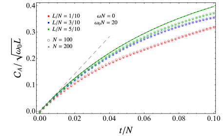
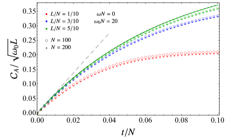
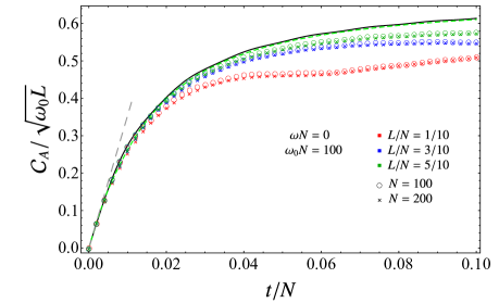
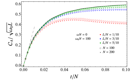
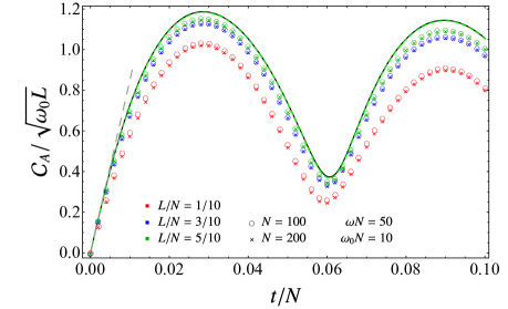
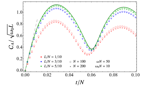
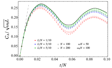
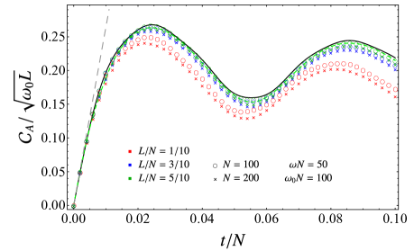
Figure 11: Initial growth of $\mathcal{C}_{A}$ in (4.6) for a block $A$ made by $L$ consecutive sites in harmonic chains with either PBC (left panels) or DBC (right panels) made by $N$ sites (in the latter case $A$ is adjacent to a boundary). When $L=N$, the complexity (3.7) is shown for $N=100$ (solid black lines) and $N=200$ (dashed green lines).

Each panel on the left in Fig. 11 is characterised by the same $\omega_{0}N$ and $\omega N$ of the corresponding one on the right. From their comparison, one realises that the qualitative behaviour of the initial growth at very early times is not influenced by the choice of the boundary conditions. Moreover, the linear growth of $\mathcal{C}_{A}/\sqrt{\omega_{0}L}$ is independent of $L/N$ for very small values of $t/N$; hence the slope of the initial growth can be found by considering the case $L=N$ (discussed in Sec. 3) and the approximation described in Sec. 3.4 and in appendix C.1. Combining these observations with (C.4) and (C.5), we obtain the initial linear growth $a_{\textrm{\tiny(B)}}\,t/N+\dots$ where the dots represent higher order in $t/N$ and the slope depends on the boundary conditions labelled by $\textrm{B}\in\{\textrm{P},\textrm{D}\}$ as follows

$$a_{\textrm{\tiny(P)}} = \frac{\big{|}(\omega N)^{2}-(\omega_{0}N)^{2}\big{|}}{2\omega_{0}N}\;\sqrt{\sqrt{\frac{m}{4\kappa}}\;\omega_{0}N\coth\!\bigg{(}\sqrt{\frac{m}{4\kappa}}\;\omega_{0}N\bigg{)}}$$ (4.8)

$$\rule{0.0pt}{31.2982pt}a_{\textrm{\tiny(D)}} = \frac{\big{|}(\omega N)^{2}-(\omega_{0}N)^{2}\big{|}}{2\sqrt{2}\omega_{0}N}\;\sqrt{\sqrt{\frac{m}{\kappa}}\;\omega_{0}N\coth\!\bigg{(}\sqrt{\frac{m}{\kappa}}\;\omega_{0}N\bigg{)}-1}\;.$$ (4.9)

The grey dashed lines in Fig. 11 represent $a_{\textrm{\tiny(P)}}\,t/N$ (left panels) and $a_{\textrm{\tiny(D)}}\,t/N$ (right panels).

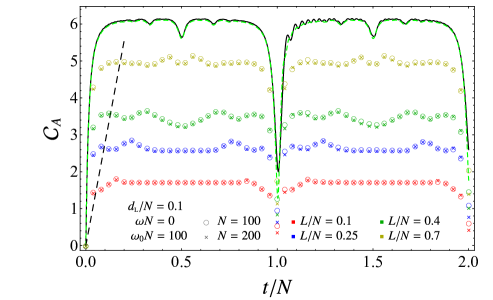
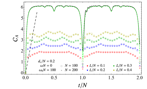
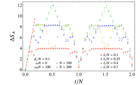
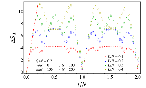
Figure 12: Temporal evolution after the global quench with a gapless evolution Hamiltonian of $\mathcal{C}_{A}$ in (4.6) (top panels) and of $\Delta S_{A}$ in (4.7) (bottom panels) for a block $A$ made by $L$ consecutive sites and separated by $d_{\textrm{\tiny L}}$ sites from the left boundary of harmonic chains with DBC made by $N$ sites. When $L=N$, the complexity (3.7) is shown for $N=100$ (solid black lines) and $N=200$ (dashed green lines).

Since for DBC and $\omega=0$ the temporal evolution of $\mathcal{C}_{A}$ displays a thermalisation regime after the initial growth and the subsequent decrease when the block $A$ with $L/N<1/2$ is adjacent to a boundary, we find it worth investigating also the case where $A$ is separated from the boundary. Denoting by $d_{\textrm{\tiny L}}$ the number of sites separating $A$ from the left boundary of the chain (hence $d_{\textrm{\tiny R}}=N-L-d_{\textrm{\tiny L}}$ sites occur between $A$ and the right boundary), $\mathcal{C}_{A}$ must be invariant under a spatial reflection w.r.t. the center of the chain, i.e. when $d_{\textrm{\tiny L}}$ and $d_{\textrm{\tiny R}}$ are replaced by $d_{\textrm{\tiny R}}-1$ and $d_{\textrm{\tiny L}}+1$ respectively.

In Fig. 12 we show the temporal evolutions of $\mathcal{C}_{A}$ and of $\Delta S_{A}$ for this bipartition of the segment when the evolution Hamiltonian is gapless and $\omega_{0}N=100$, for four different values of $L/N$ and fixed values of $d_{\textrm{\tiny L}}/N$ given by $d_{\textrm{\tiny L}}/N=0.1$ (left panels) or $d_{\textrm{\tiny L}}/N=0.2$ (right panels). Once these parameters have been chosen, the data points corresponding to $N=100$ and $N=200$ nicely collapse on the same curve.

When $d_{\textrm{\tiny L}}\neq 0$, a thermalisation regime where both the curves of $\mathcal{C}_{A}$ and $\Delta S_{A}$ are constant occurs if $b/N<1/2$, with $b=\textrm{min}[d_{\textrm{\tiny L}}+L,d_{\textrm{\tiny R}}+L-1]$ (see the red and blue curves in Fig. 12). The plateau is observed approximatively for $t/N\in[b/N,1-b/N]$ and its height depends on $\omega_{0}L$, on $L/N$ and also on $d_{\textrm{\tiny L}}/N$. A remarkable feature of the temporal evolution of $\mathcal{C}_{A}$ when $d_{\textrm{\tiny L}}>0$ is the occurrence of two local maxima for $t/N<1/2$, while only one maximum is observed when $d_{\textrm{\tiny L}}=0$ for $t/N<1/2$ (see the top panels in Fig. 7). For any given value of $L/N\leqslant 1/2$ in the top panels of Fig. 12, the subsystem complexity grows in the temporal regime between the two local maxima, for $t/N<1/2$. The occurrence of two local maxima in the temporal evolution of $\mathcal{C}_{A}$ when $A$ is separated from the boundary is observed also when $N\to\infty$. This is shown in Fig. 14 and Fig. 16, where we also highlight the logarithmic nature of the growth of $\mathcal{C}_{A}$ in the temporal regime between the two local maxima, which can be compared with a logarithmic growth occurring in $\Delta S_{A}$ (see e.g. Fig. 15).

Comparing each top panel with the corresponding bottom panel in Fig. 12, we observe that the black dashed straight line (it is the same in the two top panels) captures the first local maximum of $\mathcal{C}_{A}$. The slope of this line is twice the slope of the red dashed straight line in the bottom panels, which identifies the initial linear growth of $\Delta S_{A}$.

5 Subsystem complexity and the generalised Gibbs ensemble

In this section we consider infinite harmonic chains, either on the infinite line or on the semi-infinite line with DBC at the origin, and discuss that the asymptotic value of $\mathcal{C}_{A}$ for a block made by consecutive sites can be found through the generalised Gibbs ensemble (GGE).

5.1 Complexity of the GGE

An isolated system prepared in a pure state and then suddenly driven out of equilibrium through a global quench does not relax. Instead, relaxation occurs for a subsystem [114, 115, 116] (see also the review [39] and the references therein).

Consider a spatial bipartition of a generic harmonic chain given by a finite subsystem $A$ and its complement. Denoting by $\hat{\rho}(t)$ the density matrix of the entire system and by $\hat{\rho}_{A}(t)$ the reduced density matrix of $A$, a quantum system relaxes locally to a stationary state if the limit $\lim_{t\to\infty}\lim_{N\to\infty}\hat{\rho}_{A}(t)\equiv\hat{\rho}_{A}(t=\infty)$ exists for any $A$, where $N$ is the number of sites in the harmonic chain. This stationary state is described by the time independent density matrix $\hat{\rho}_{\textrm{\tiny E}}$ describing a statistical ensemble if $\lim_{N\to\infty}\hat{\rho}_{\textrm{\tiny E},A}=\hat{\rho}_{A}(t=\infty)$, for any $A$, where $\hat{\rho}_{\textrm{\tiny E},A}$ is obtained by tracing $\hat{\rho}_{\textrm{\tiny E}}$ over the degrees of freedom of the complement of $A$. For the global quench of the mass parameter that we are investigating in infinite harmonic chains, the stationary state is described by a GGE [44, 117, 45, 118] (see the review [46] for an extensive list of references).

In terms of the creation and annihilation operators (A.8), the evolution Hamiltonian reads

$$\widehat{H}=\sum_{k=1}^{N}\Omega_{k}\!\left(\hat{\mathfrak{b}}_{k}^{\dagger}\,\hat{\mathfrak{b}}_{k}+\frac{1}{2}\,\right).$$ (5.1)

The GGE that provides the stationary state reads [43]

$$\hat{\rho}_{\textrm{\tiny GGE}}=\frac{e^{-\sum_{k=1}^{N}\lambda_{k}\hat{\mathfrak{b}}_{k}^{\dagger}\hat{\mathfrak{b}}_{k}}}{\mathcal{Z}_{\textrm{\tiny GGE}}}\;\;\qquad\;\;\mathcal{Z}_{\textrm{\tiny GGE}}=\textrm{Tr}(\hat{\rho}_{\textrm{\tiny GGE}})=\prod_{k=1}^{N}\frac{1}{1-e^{-\lambda_{k}}}$$ (5.2)

where $\hat{\rho}_{\textrm{\tiny GGE}}$ is normalised through the condition $\textrm{Tr}(\hat{\rho}_{\textrm{\tiny GGE}})=1$. The conservation of the number operators $\hat{\mathfrak{b}}_{k}^{\dagger}\hat{\mathfrak{b}}_{k}$ tells us that the relation between their expectation values and $\lambda_{k}$ reads [43]

$$n_{k}\,\equiv\,\textrm{Tr}\big{(}\hat{\mathfrak{b}}_{k}^{\dagger}\,\hat{\mathfrak{b}}_{k}\,\hat{\rho}_{\textrm{\tiny GGE}}\big{)}=\frac{1}{e^{\lambda_{k}}-1}\,=\,\langle\psi_{0}|\,\hat{\mathfrak{b}}_{k}^{\dagger}\,\hat{\mathfrak{b}}_{k}\,|\psi_{0}\rangle$$ (5.3)

which is strictly positive because $\lambda_{k}>0$ for any value of $k$.

Since the GGE in (5.2) is a bosonic Gaussian state, it is characterised by its covariance matrix $\gamma_{\textrm{\tiny GGE}}$, which can be decomposed as follows

$$\gamma_{\textrm{\tiny GGE}}=\,\bigg{(}\begin{array}[]{cc}Q_{\textrm{\tiny GGE}}&\,M_{\textrm{\tiny GGE}}\\ M_{\textrm{\tiny GGE}}^{\textrm{t}}&\,P_{\textrm{\tiny GGE}}\end{array}\bigg{)}$$ (5.4)

where (see the appendix A.3)

$$(Q_{\textrm{\tiny GGE}})_{i,j}=\textrm{Tr}\big{(}\hat{q}_{i}\,\hat{q}_{j}\,\hat{\rho}_{\textrm{\tiny GGE}}\big{)}\qquad(P_{\textrm{\tiny GGE}})_{i,j}=\textrm{Tr}\big{(}\hat{p}_{i}\,\hat{p}_{j}\,\hat{\rho}_{\textrm{\tiny GGE}}\big{)}\qquad(M_{\textrm{\tiny GGE}})_{i,j}=\textrm{Re}\big{[}\textrm{Tr}\big{(}\hat{q}_{i}\,\hat{p}_{j}\,\hat{\rho}_{\textrm{\tiny GGE}}\big{)}\big{]}\,.$$ (5.5)

By adapting the computation reported in appendix A.1 to this case, the operators $\hat{\boldsymbol{\mathfrak{q}}}$ and $\hat{\boldsymbol{\mathfrak{p}}}$ can be introduced as in (A.7) and for (5.4) one finds

$$Q_{\textrm{\tiny GGE}} = \widetilde{V}\,S^{-1}_{\textrm{\tiny phys}}\,\textrm{Tr}\big{(}\hat{\boldsymbol{\mathfrak{q}}}\,\hat{\boldsymbol{\mathfrak{q}}}^{\textrm{t}}\hat{\rho}_{\textrm{\tiny GGE}}\big{)}\,S^{-1}_{\textrm{\tiny phys}}\,\widetilde{V}^{\textrm{t}}\equiv\widetilde{V}\,\mathcal{Q}\textrm{\tiny GGE}\,\widetilde{V}^{\textrm{t}}$$ (5.6)

$$\rule{0.0pt}{14.22636pt}P_{\textrm{\tiny GGE}} = \widetilde{V}\,S_{\textrm{\tiny phys}}\,\textrm{Tr}\big{(}\hat{\boldsymbol{\mathfrak{p}}}\,\hat{\boldsymbol{\mathfrak{p}}}^{\textrm{t}}\hat{\rho}_{\textrm{\tiny GGE}}\big{)}\,S_{\textrm{\tiny phys}}\,\widetilde{V}^{\textrm{t}}\,\equiv\,\widetilde{V}\,\mathcal{P}\textrm{\tiny GGE}\,\widetilde{V}^{\textrm{t}}$$ (5.7)

$$\rule{0.0pt}{14.22636pt}M_{\textrm{\tiny GGE}} = \widetilde{V}\,S^{-1}_{\textrm{\tiny phys}}\,\textrm{Re}\big{[}\textrm{Tr}\big{(}\hat{\boldsymbol{\mathfrak{q}}}\,\hat{\boldsymbol{\mathfrak{p}}}^{\textrm{t}}\hat{\rho}_{\textrm{\tiny GGE}}\big{)}\big{]}\,S_{\textrm{\tiny phys}}\,\widetilde{V}^{\textrm{t}}\,\equiv\,\widetilde{V}\,\mathcal{M}\textrm{\tiny GGE}\,\widetilde{V}^{\textrm{t}}\,.$$ (5.8)

Then, expressing $\hat{\boldsymbol{\mathfrak{q}}}$ and $\hat{\boldsymbol{\mathfrak{p}}}$ in terms of $\hat{\boldsymbol{\mathfrak{b}}}$ and $\hat{\boldsymbol{\mathfrak{b}}}^{\dagger}$ defined in (A.8), exploiting the fact that the two points correlators vanish when the indices of the annihilation and creation operators are different, using (5.3) and $\textrm{Tr}\big{(}\hat{\mathfrak{b}}_{k}^{\dagger}\hat{\mathfrak{b}}_{k}^{\dagger}\,\hat{\rho}_{\textrm{\tiny GGE}}\big{)}=\textrm{Tr}\big{(}\hat{\mathfrak{b}}_{k}\hat{\mathfrak{b}}_{k}\hat{\rho}_{\textrm{\tiny GGE}}\big{)}=0$, we find $M\textrm{\tiny GGE}=\mathcal{M}\textrm{\tiny GGE}=\mathbf{0}$ and

$$\mathcal{Q}_{\textrm{\tiny GGE}}\,\equiv\,\textrm{diag}\,\Big{\{}Q_{\textrm{\tiny GGE},k}\,;1\leqslant k\leqslant N\Big{\}}\;\;\qquad\;\;\mathcal{P}_{\textrm{\tiny GGE}}\,\equiv\,\textrm{diag}\,\Big{\{}P_{\textrm{\tiny GGE},k}\,;1\leqslant k\leqslant N\Big{\}}$$ (5.9)

where

$$Q_{\textrm{\tiny GGE},k}\equiv\frac{1+2n_{k}}{2m\,\Omega_{k}}\;\;\qquad\;\;P_{\textrm{\tiny GGE},k}\equiv\frac{m\,\Omega_{k}}{2}\,(1+2n_{k})\,.$$ (5.10)

Thus, the covariance matrix (5.4) simplifies to $\gamma_{\textrm{\tiny GGE}}=Q_{\textrm{\tiny GGE}}\oplus P_{\textrm{\tiny GGE}}$, where $Q\textrm{\tiny GGE}$ and $P\textrm{\tiny GGE}$ are given by (5.6) and (5.7).

We find it worth writing the Williamson’s decomposition of $\gamma_{\textrm{\tiny GGE}}$, namely

$$\gamma_{\textrm{\tiny GGE}}\,=\,W^{\textrm{t}}_{\textrm{\tiny GGE}}\,\mathcal{D}_{\textrm{\tiny GGE}}\,W_{\textrm{\tiny GGE}}\,\,\qquad\,\,W_{\textrm{\tiny GGE}}=\mathcal{X}_{\textrm{\tiny GGE}}\,V^{\textrm{t}}$$ (5.11)

where the symplectic spectrum is given by

$$\mathcal{D}_{\textrm{\tiny GGE}}=\frac{1}{2}\,\boldsymbol{1}+\textrm{diag}\,\Big{\{}n_{1},\dots,n_{N},n_{1},\dots,n_{N}\Big{\}}$$ (5.12)

and, like for the $2N\times 2N$ symplectic matrix $W_{\textrm{\tiny GGE}}$, we have $V=\widetilde{V}\oplus\widetilde{V}$ and that the diagonal matrix $\mathcal{X}_{\textrm{\tiny GGE}}=\mathcal{X}_{\textrm{\tiny phys}}^{-1}$ is the inverse of $\mathcal{X}_{\textrm{\tiny phys}}$ defined in (A.4). We emphasise that $\gamma_{\textrm{\tiny GGE}}$ does not describe a pure state. Indeed, since $n_{k}\geqslant 0$ for any $k$, from (5.12) we have that the symplectic eigenvalues of $\gamma_{\textrm{\tiny GGE}}$ are greater than $1/2$, as expected for a mixed bosonic Gaussian state.

For the global quench in the harmonic chains that we considering, $n_{k}$ in (5.3) can be computed from the expectation value of $\hat{\mathfrak{b}}_{k}^{\dagger}\hat{\mathfrak{b}}_{k}$ on the initial state obtaining [43]

$$n_{k}=\frac{1}{4}\bigg{(}\frac{\Omega_{k}}{\Omega_{0,k}}+\frac{\Omega_{0,k}}{\Omega_{k}}\bigg{)}-\frac{1}{2}$$ (5.13)

where $\Omega_{0,k}$ and $\Omega_{k}$ are the dispersion relations of the Hamiltonian defining the initial state and of the evolution Hamiltonian respectively. Notice that (5.13) is symmetric under the exchange $\Omega_{k}\leftrightarrow\Omega_{0,k}\,$. We recall that the boundary conditions defining the harmonic chain influence both the dispersion relations and the matrix $V$.

By introducing the reduced covariance matrix $\gamma_{\textrm{\tiny GGE},A}$ for $A$, obtained from (5.4) in the usual way, the entanglement entropy

$$S_{\textrm{\tiny GGE},A}\equiv-\textrm{Tr}(\hat{\rho}_{\textrm{\tiny GGE},A}\log\hat{\rho}_{\textrm{\tiny GGE},A})$$ (5.14)

can be evaluated from the symplectic spectrum of $\gamma_{\textrm{\tiny GGE},A}$ through standard methods [106, 57].

The asymptotic value of the increment of the entanglement entropy $\Delta S_{A}$ when $t\to\infty$ can be computed as follows

$$\lim_{L\to\infty}\frac{\lim_{t\to\infty}\lim_{N\to\infty}\Delta S_{A}}{L}=\lim_{L\to\infty}\frac{\lim_{N\to\infty}S_{\textrm{\tiny GGE},A}}{L}=\lim_{N\to\infty}\frac{S_{\textrm{\tiny GGE}}}{N}$$ (5.15)

where the order of the limits is important and in the last step we used that $S_{\textrm{\tiny GGE}}$ is an extensive quantity (see the review [119] and the references therein).

For the global quench in the harmonic chains that we are considering, the asymptotic value (5.15) for the entanglement entropy reads [63]

$$\lim_{N\to\infty}\frac{S_{\textrm{\tiny GGE}}}{N} = \int_{0}^{\pi}\Big{[}(n_{\theta}+1)\log(n_{\theta}+1)-n_{\theta}\log n_{\theta}\Big{]}\,\frac{d\theta}{\pi}$$ (5.16)

$$= \int_{0}^{\pi}\Bigg{\{}\bigg{[}\frac{1}{4}\bigg{(}\frac{\Omega_{\theta}}{\Omega_{0,\theta}}+\frac{\Omega_{0,\theta}}{\Omega_{\theta}}\bigg{)}+\frac{1}{2}\bigg{]}\log\!\bigg{[}\frac{1}{4}\bigg{(}\frac{\Omega_{\theta}}{\Omega_{0,\theta}}+\frac{\Omega_{0,\theta}}{\Omega_{\theta}}\bigg{)}+\frac{1}{2}\bigg{]}$$ (5.17)

$$\hskip 28.45274pt-\,\bigg{[}\frac{1}{4}\bigg{(}\frac{\Omega_{\theta}}{\Omega_{0,\theta}}+\frac{\Omega_{0,\theta}}{\Omega_{\theta}}\bigg{)}-\frac{1}{2}\bigg{]}\log\!\bigg{[}\frac{1}{4}\bigg{(}\frac{\Omega_{\theta}}{\Omega_{0,\theta}}+\frac{\Omega_{0,\theta}}{\Omega_{\theta}}\bigg{)}-\frac{1}{2}\bigg{]}\Bigg{\}}\,\frac{d\theta}{\pi}$$

in terms of $n_{\theta}$ given in (5.13), where the dispersion relations to employ are (3.24) for PBC and (3.25) for DBC. A straightforward change of integration variable leads to the same expression for both the boundary conditions, as already noticed for (3.23). Let us remark that (5.16) is finite for any choice of the parameter (including $\omega=0$), both for PBC and DBC. It is also symmetric under the exchange $\Omega_{\theta}\leftrightarrow\Omega_{0,\theta}$; hence under $\omega\leftrightarrow\omega_{0}$ as well.

We study the circuit complexity to construct the GGE (which is a mixed state) starting from the (pure) initial state at $t=0$, by employing the approach based on the Fisher information geometry [74]. The optimal circuit to get $\gamma_{\textrm{\tiny GGE}}$ from the initial covariance matrix $\gamma(0)$ at $t=0$ reads [95, 74]

$$G_{s}(\gamma(0)\,,\gamma_{\textrm{\tiny GGE}})\,\equiv\,\gamma(0)^{1/2}\Big{(}\gamma(0)^{-1/2}\,\gamma_{\textrm{\tiny GGE}}\,\gamma(0)^{-1/2}\Big{)}^{s}\gamma(0)^{1/2}$$ (5.18)

where $0\leqslant s\leqslant 1$ parameterises the covariance matrix along the circuit. The length of the optimal circuit (5.18) provides the circuit complexity

$$\mathcal{C}_{\textrm{\tiny GGE}}\,=\,\frac{1}{2\sqrt{2}}\;\sqrt{\textrm{Tr}\,\Big{\{}\big{[}\log\!\big{(}\gamma_{\textrm{\tiny GGE}}\;\gamma(0)^{-1}\big{)}\big{]}^{2}\Big{\}}}\;.$$ (5.19)

Since $\mathcal{M}_{\textrm{\tiny GGE}}=\mathcal{M}(0)=\boldsymbol{0}$, from (2.5), (5.6) and (5.7) we obtain

$$\gamma_{\textrm{\tiny GGE}}=V\big{[}\mathcal{Q}_{\textrm{\tiny GGE}}\oplus\mathcal{P}_{\textrm{\tiny GGE}}\big{]}V^{\textrm{t}}\;\;\qquad\;\;\gamma(0)=V\big{[}\mathcal{Q}(0)\oplus\mathcal{P}(0)\big{]}V^{\textrm{t}}\,.$$ (5.20)

Then, by exploiting (5.9), (2.7) and the fact that the matrix $V$ is the same for both $\gamma_{\textrm{\tiny GGE}}$ and $\gamma(0)$, we find that the complexity (5.19) reads

$$\mathcal{C}_{\textrm{\tiny GGE}} = \frac{1}{2\sqrt{2}}\;\sqrt{\,\sum_{k=1}^{N}\bigg{\{}\bigg{[}\log\bigg{(}\frac{Q_{\textrm{\tiny GGE},k}}{Q_{k}(0)}\bigg{)}\bigg{]}^{2}+\bigg{[}\log\bigg{(}\frac{P_{\textrm{\tiny GGE},k}}{P_{k}(0)}\bigg{)}\bigg{]}^{2}\Bigg{\}}}$$ (5.21)

$$= \frac{1}{2\sqrt{2}}\;\sqrt{\,\sum_{k=1}^{N}\Bigg{\{}\bigg{[}\log\bigg{(}\frac{\Omega_{0,k}}{\Omega_{k}}\,(1+2n_{k})\bigg{)}\bigg{]}^{2}+\bigg{[}\log\bigg{(}\frac{\Omega_{k}}{\Omega_{0,k}}\,(1+2n_{k})\bigg{)}\bigg{]}^{2}\Bigg{\}}}\;.$$ (5.22)

By using (5.13), this expression becomes

$$\mathcal{C}_{\textrm{\tiny GGE}}\,=\,\frac{1}{2\sqrt{2}}\;\sqrt{\,\sum_{k=1}^{N}\Bigg{\{}\bigg{[}\log\bigg{(}\frac{\Omega_{0,k}^{2}}{2\,\Omega_{k}^{2}}+\frac{1}{2}\bigg{)}\bigg{]}^{2}+\bigg{[}\log\bigg{(}\frac{\Omega_{k}^{2}}{2\,\Omega_{0,k}^{2}}+\frac{1}{2}\bigg{)}\bigg{]}^{2}\Bigg{\}}}$$ (5.23)

which is symmetric under the exchange $\Omega_{k}\leftrightarrow\Omega_{0,k}$, hence under $\omega\leftrightarrow\omega_{0}$ as well.

The leading order of this expression as $N\to\infty$ is given by

$$\mathcal{C}_{\textrm{\tiny GGE}}=\frac{\sqrt{N}}{2\,\sqrt{2\pi}}\;\sqrt{\,\int_{0}^{\pi}\left\{\bigg{[}\log\bigg{(}\frac{\Omega_{0,\theta}^{2}}{2\,\Omega_{\theta}^{2}}+\frac{1}{2}\bigg{)}\bigg{]}^{2}+\bigg{[}\log\bigg{(}\frac{\Omega_{\theta}^{2}}{2\,\Omega_{0,\theta}^{2}}+\frac{1}{2}\bigg{)}\bigg{]}^{2}\right\}\,d\theta}$$ (5.24)

where $\Omega_{0,\theta}$ and $\Omega_{\theta}$ are thermodynamic limits of the dispersion relations associated to the Hamiltonians before and after the quench respectively. By repeating the argument reported below (3.23), one finds that (5.24) with (3.24) can be employed for both PBC and DBC. Moreover, the resulting expression for $\mathcal{C}_{\textrm{\tiny GGE}}/\sqrt{N}$ is finite for any choice of the parameters (including for $\omega=0$).

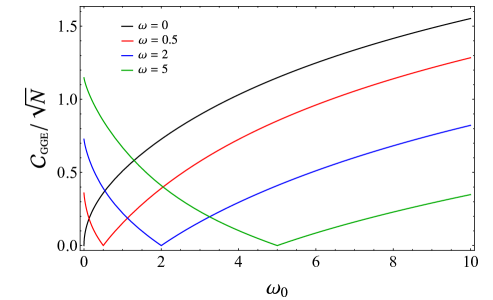
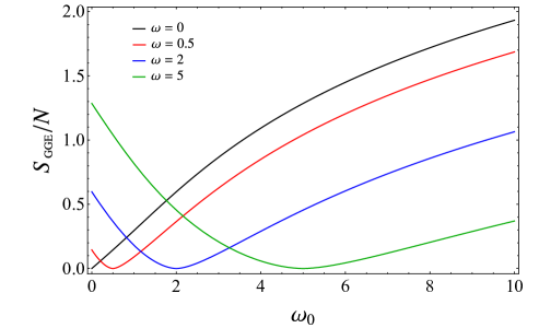
Figure 13: Asymptotic value of $\mathcal{C}_{\textrm{\tiny GGE}}/\sqrt{N}$ from (5.24) (left panel) and of $S_{\textrm{\tiny GGE}}/N$ from (5.16) (right panel) as functions of $\omega_{0}$, for some values of $\omega$.

In Fig. 13 we show $\mathcal{C}_{\textrm{\tiny GGE}}/\sqrt{N}$ from (5.24) and $S_{\textrm{\tiny GGE}}/N$ from (5.16) as functions of $\omega_{0}$, for some values of $\omega$. The resulting curves are qualitatively similar. At $\omega_{0}=\omega$ they both vanish, but $\mathcal{C}_{\textrm{\tiny GGE}}/\sqrt{N}$ is singular at this point, while $S_{\textrm{\tiny GGE}}/N$ is smooth.

The reduced covariance matrix $\gamma_{\textrm{\tiny GGE},A}$ associated to any finite subsystem $A$ is obtained by selecting the rows and the columns in (5.4) corresponding to $A$. The results of [74] can be applied again to write the optimal circuit that provides $\gamma_{\textrm{\tiny GGE},A}$ from the initial mixed state characterised by the reduced covariance matrix $\gamma_{A}(0)$ at $t=0$, obtained from $\gamma(0)$ through the usual reduction procedure. This optimal circuit reads

$$G_{s}(\gamma_{A}(0)\,,\gamma_{\textrm{\tiny GGE},A})\,\equiv\,\gamma_{A}(0)^{1/2}\Big{(}\gamma_{A}(0)^{-1/2}\,\gamma_{\textrm{\tiny GGE},A}\,\gamma_{A}(0)^{-1/2}\Big{)}^{s}\gamma_{A}(0)^{1/2}$$ (5.25)

where $0\leqslant s\leqslant 1$ parametrises the covariance matrix along the optimal circuit. Its length corresponds to the subsystem complexity of the GGE w.r.t. the initial state

$$\mathcal{C}_{\textrm{\tiny GGE},A}\,=\,\frac{1}{2\sqrt{2}}\;\sqrt{\textrm{Tr}\,\Big{\{}\big{[}\log\!\big{(}\gamma_{\textrm{\tiny GGE},A}\,\gamma_{A}(0)^{-1}\big{)}\big{]}^{2}\Big{\}}}\;.$$ (5.26)

Since the harmonic chain relaxes locally to the GGE after the quantum quench, for the subsystem complexity of any finite subsystem $A$ we expect

$$\lim_{t\to\infty}\,\lim_{N\to\infty}\mathcal{C}_{A}=\lim_{N\to\infty}\mathcal{C}_{\textrm{\tiny GGE},A}$$ (5.27)

which is confirmed by the numerical results in Fig. 14, Fig. 16, Fig. 19, Fig. 20 and Fig. 21.

A numerical analysis shows that (5.27) grows like $\sqrt{L}$ as $L\to\infty$ for fixed values of $\omega$ and $\omega_{0}$; hence, by adapting (5.15) to the subsystem complexity, we expect

$$\lim_{L\to\infty}\frac{\lim_{t\to\infty}\lim_{N\to\infty}\mathcal{C}_{A}}{\sqrt{L}}=\lim_{L\to\infty}\frac{\lim_{N\to\infty}\mathcal{C}_{\textrm{\tiny GGE},A}}{\sqrt{L}}=\lim_{N\to\infty}\frac{\mathcal{C}_{\textrm{\tiny GGE}}}{\sqrt{N}}$$ (5.28)

where $\mathcal{C}_{\textrm{\tiny GGE}}$ is given in (5.24) and the order of the limits is important. Numerical evidences for (5.28) are discussed in appendix D (see Fig. 22 and Fig. 23).

In the following numerical analysis we show that, for the harmonic chains that we are exploring, the asymptotic limit for $t\to\infty$ of the reduced density matrix after the global quench is the reduced density matrix obtained from the GGE. This result has been already discussed for a fermionic chain in [120], where, considering a global quench of the magnetic field in the transverse-field Ising chain and the subsystem given by a finite block made by consecutive sites in an infinite chain on the line, it has been found that a properly defined distance between the reduced density matrix at a generic value of time along the evolution and the asymptotic one obtained from the GGE vanishes as $t\to\infty$.

5.2 Numerical results

In order to test (5.26), infinite harmonic chains must be considered. The reference and the target states have been described in Sec. 4. In this section we study harmonic chains both on the line and on the semi-infinite line with DBC imposed at its origin. In the latter case, the block $A$ made by $L$ consecutive sites is either adjacent to the origin or separated from it.

The correlators to employ in the numerical analysis can be obtained from the ones reported in Sec. 4. For the infinite harmonic chain on the line, we take $N\to\infty$ of (4.1), finding

$$\begin{array}[]{l}\displaystyle Q_{i,j}(t)=\frac{1}{\pi}\int_{0}^{\pi}Q_{\theta}(t)\cos\!\big{[}2\theta\,(i-j)\,\big{]}\,d\theta\\ \rule{0.0pt}{25.6073pt}\displaystyle P_{i,j}(t)=\frac{1}{\pi}\int_{0}^{\pi}P_{\theta}(t)\cos\!\big{[}2\theta\,(i-j)\,\big{]}\,d\theta\\ \displaystyle\rule{0.0pt}{25.6073pt}\displaystyle M_{i,j}(t)=\,\frac{1}{\pi}\int_{0}^{\pi}M_{\theta}(t)\cos\!\big{[}2\theta\,(i-j)\,\big{]}\,d\theta\end{array}$$ (5.29)

where $i,j\in\mathbb{Z}$; while, for the harmonic chain on the semi-infinite line with DBC, the limit $N\to\infty$ of (4.1) leads to

$$\begin{array}[]{l}\displaystyle Q_{i,j}(t)=\frac{2}{\pi}\int_{0}^{\pi}Q_{\theta}(t)\sin(i\theta)\sin(j\theta)\,d\theta\\ \rule{0.0pt}{25.6073pt}\displaystyle P_{i,j}(t)=\frac{2}{\pi}\int_{0}^{\pi}P_{\theta}(t)\sin(i\theta)\sin(j\theta)\,d\theta\\ \displaystyle\rule{0.0pt}{25.6073pt}\displaystyle M_{i,j}(t)=\frac{2}{\pi}\int_{0}^{\pi}M_{\theta}(t)\sin(i\theta)\sin(j\theta)\,d\theta\end{array}$$ (5.30)

where $i,j>0$. The functions $Q_{\theta}(t)$, $P_{\theta}(t)$ and $M_{\theta}(t)$ in these integrands are given by (2.6) where $\Omega_{0,k}$ and $\Omega_{k}$ are replaced respectively by $\Omega_{0,\theta}$ and $\Omega_{\theta}$, which are (3.24) and (3.25) for the infinite and for the semi-infinite line respectively.

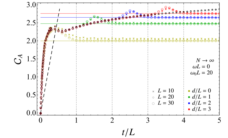
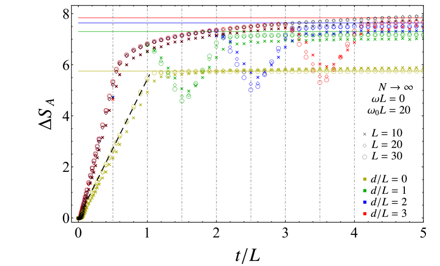
Figure 14: Temporal evolution of $\mathcal{C}_{A}$ (top panel) and of $\Delta S_{A}$ (bottom panel) after a global quantum quench with a gapless evolution Hamiltonian and $\omega_{0}L=20$. The subsystem is a block $A$ made by $L$ consecutive sites either on the infinite line (black data points) or on the semi-infinite line, separated by $d$ sites from the origin where DBC hold (coloured data points). The dashed black straight line is the same in both panels.

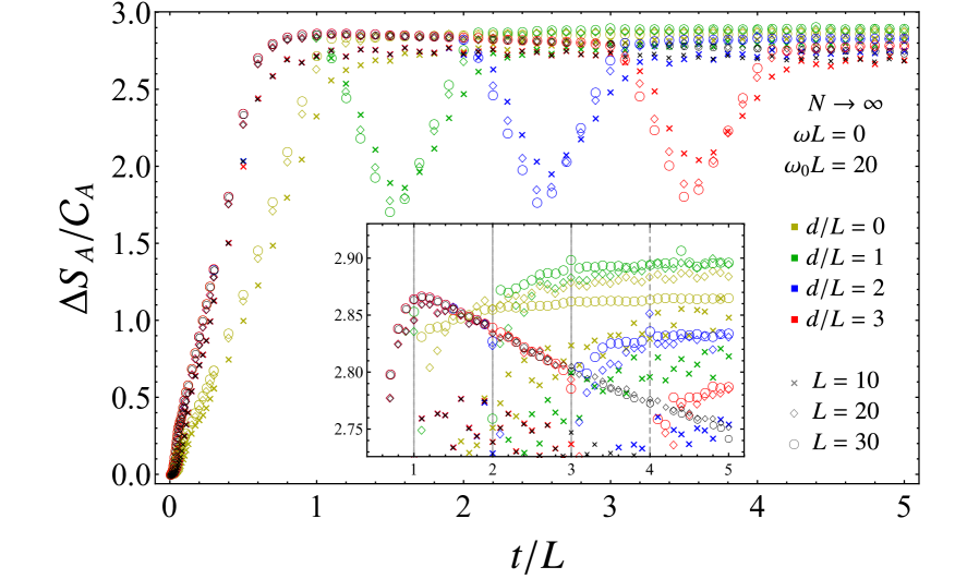
Figure 15: Temporal evolution of $\Delta S_{A}/\mathcal{C}_{A}$ for the data reported in Fig. 14. The inset zooms in to highlight the data points having $t/L>1$.

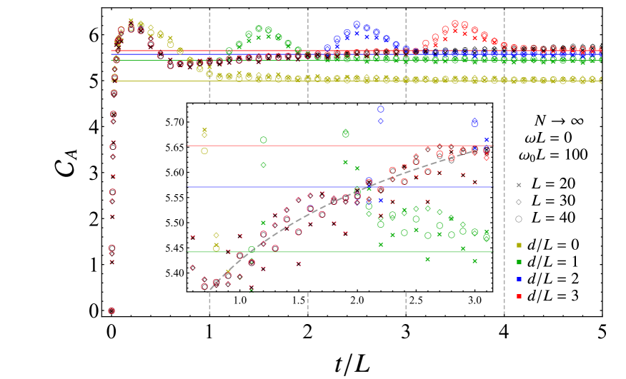
Figure 16: Temporal evolution of $\mathcal{C}_{A}$ after a global quantum quench with a gapless evolution Hamiltonian and $\omega_{0}L=100$, in the same setups of Fig. 14. The inset zooms in on the intermediate temporal regime between the two local maxima for the data having $d/L=3$.

Once the proper correlators on the chain are identified, the reduced correlation matrices $Q_{A}$, $P_{A}$ and $M_{A}$ are the blocks providing the reduced covariance matrix (4.1). These matrices are obtained by restricting the indices of the proper correlators to $i,j=1,\dots,L$ when $A$ is on the infinite line and to $i,j=1+d,\dots,L+d$ when $A$ is on the semi-infinite line, where $d$ corresponds to its separation from the origin.

In the following we discuss numerical data sets obtained for infinite harmonic chains, either on the infinite line or on the semi-infinite line, where $\omega L$ and $\omega_{0}L$ are kept fixed. In appendix D we report numerical results characterised by fixed values of $\omega$ and $\omega_{0}$.

In Fig. 14 and Fig. 15 we show the temporal evolutions of $\mathcal{C}_{A}$, of $\Delta S_{A}$ and of $\Delta S_{A}/\mathcal{C}_{A}$ after the quench with $\omega_{0}L=20$ and $\omega L=0$. In Fig. 16 we display the temporal evolution of $\mathcal{C}_{A}$ with $\omega_{0}L=100$ and $\omega L=0$. The subsystem $A$ is a block made by $L$ consecutive sites either on a semi-infinite line, separated by $d$ sites from the origin where DBC are imposed (coloured symbols), or on the infinite line (black symbols). The black and coloured data points for $\mathcal{C}_{A}$ have been found through (4.6) with the reduced correlators obtained from either (5.29) or (5.30) respectively. The coloured horizontal solid lines correspond to either (5.26) or (5.14), with the reduced correlators from (A.34) for the target state and from (5.30) at $t=0$ for the reference state, with $L=50$. Notice that a black horizontal solid line does not occur because the corresponding value is divergent, as indicated also by the left panel in Fig. 17.

Considering the block on the semi-infinite line, in Fig. 14 and Fig. 16 we observe that the initial growth of $\mathcal{C}_{A}$ is the same until the first local maximum, for all the values of $d/L$. After the first local maximum, the temporal evolution of $\mathcal{C}_{A}$ depends on whether the block is adjacent to the boundary. If $d/L=0$ the curve decreases until it reaches the saturation value. Instead, when $d/L>0$, first $\mathcal{C}_{A}$ decreases along a different curve (see e.g. Fig. 16) until a local minimum; then we observe an intermediate growth, followed by a second local maximum and finally by the saturation regime. A fitting procedure shows that the intermediate growth between the two local maxima is logarithmic (in the inset of Fig. 16 the grey dashed curve has been found by fitting the data having $L=40$ and $d/L=3$ through a logarithm and a constant). Its temporal duration is approximatively $d/L-1/2$, for the three values of non vanishing $d/L$ considered in Fig. 14 and Fig. 16. Fitting the intermediate growth in Fig. 14 and Fig. 16, one observes that the coefficient of the logarithmic growth decreases as $\omega_{0}L$ increases. The first local maximum in the temporal evolution of $\mathcal{C}_{A}$ occurs for $0<t/L<1$. When $d>0$, the second maximum occurs for $d/L<t/L<(d+1)/L$. Notice that these two local maxima can be seen also in the top panels of Fig. 12 for $t/N<1/2$.

In Fig. 14, Fig. 15 and Fig. 16, the data points represented through black symbols have been obtained for a block in the infinite line. These data overlap with the ones corresponding to the block on the semi-infinite line with $d>0$ until the latter ones display the development of the second local maximum. For the temporal evolution of $\mathcal{C}_{A}$ on the infinte line only one local maximum occurs and the intermediate logarithmic growth mentioned above does not finish within the temporal regime that we have considered. This agreement tells us that the second local maximum in the temporal evolution of $\mathcal{C}_{A}$ is due to the presence of the boundary.

The temporal evolutions of $\Delta S_{A}$ in the bottom panel of Fig. 14 can be explained by employing the quasi-particle picture [41], which provides the different temporal regimes and the corresponding qualitative behaviour of $\Delta S_{A}$ (for the subsystems where a boundary occurs, the quasi-particle picture has been described e.g. in [68]). The different regimes identified by this analysis correspond to the vertical dot-dashed lines in the bottom panel of Fig. 14. Instead, the vertical dashed grey lines in the top panel of Fig. 14 correspond to $t/L=1+d/L$. For $d>0$, when $t/L>1/2$ we observe a regime of logarithmic growth for $\Delta S_{A}$ whose duration depends on $d/L$ according to the quasi-particle picture, until the beginning of a linear decreases. Considering two sets of data points of $\Delta S_{A}$ having different $d/L$, they collapse until the first linear decrease is reached.

The initial growths of $\mathcal{C}_{A}$ and of $\Delta S_{A}$ in Fig. 14 are very different. For instance, the growth of $\mathcal{C}_{A}$ is the same for all the data sets, while for $\Delta S_{A}$ it depends on whether $d$ vanishes. Moreover, while the growth of $\Delta S_{A}$ is linear for $t/L<1$ when $d=0$ and for $t/L<1/2$ when $d>0$, the growth of $\mathcal{C}_{A}$ is linear only at the very beginning of the temporal evolution and it clearly deviates from linearity within the regime of $t/L$ where $\Delta S_{A}$ grows linearly. The dashed black straight line passing through the origin in Fig. 14 describes the linear growth of $\Delta S_{A}$ when $d=0$ and it is the same in both the panels. This straight line intersects the first local maximum of $\mathcal{C}_{A}$. This has been highlighted also for finite systems in Fig. 7 and Fig. 12.

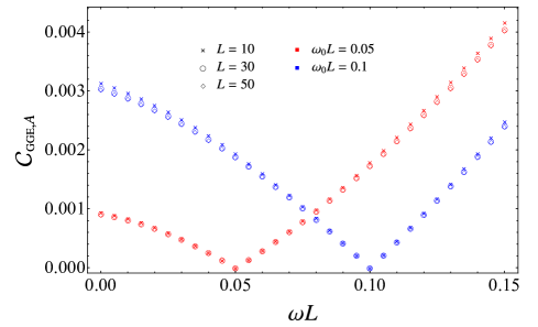
Figure 17: Asymptotic value of $\mathcal{C}_{\textrm{\tiny GGE},A}$ in (5.26) for a block $A$ made by $L$ consecutive sites in infinite chains in terms of $\omega L$. The block is either in an infinite chain (left panel) or adjacent to the origin of the semi-infinite line with DBC (right panel).

In Fig. 15 we show the ratio $\Delta S_{A}/\mathcal{C}_{A}$ for the data reported in Fig. 14. We remark that the two logarithmic growths occurring in $\Delta S_{A}$ and in $\mathcal{C}_{A}$ almost cancel in the ratio; indeed, a mild logarithmic decreasing is observed when $t/L>1$ for the data obtained on the infinite line (black symbols) and when $1<t/L<3$ for the data obtained on the semi-infinite line with $d/L=3$ (red symbols) that are already collapsed.

The curves in Fig. 16 must be compared with the corresponding ones in top panel in Fig. 14 in order to explore the effect of $\omega_{0}L$. The height of the first local maximum in the temporal evolution of $\mathcal{C}_{A}$ and also the saturation values for the data obtained on the semi-infinite line increase as $\omega_{0}L$ increases. Instead, the coefficient of the logarithmic growth after the first local maximum decreases as $\omega_{0}L$ increases, as already remarked above. Notice that higher values of $L$ are needed to observe data collapse as $\omega_{0}L$ increases.

From the numerical results reported in the previous figures, we conclude that (5.26) provides the asymptotic value of the subsystem complexity as $t\to\infty$; hence it is worth studying the dependence of this expression on the subsystem size and on the parameters of the quench protocol.

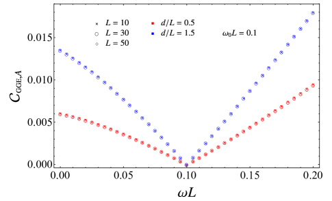
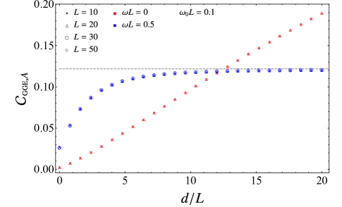
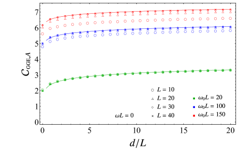
Figure 18: Asymptotic value of $\mathcal{C}_{\textrm{\tiny GGE},A}$ in (5.26) for a block made by $L$ consecutive sites and separated by $d$ sites from the origin of a semi-infinite line with DBC, in terms of $\omega L$ (top panel) and of $d/L$ (bottom panels).

In Fig. 17 and Fig. 18 we show numerical results for (5.26), obtained by using the reduced correlators from (A.31) and (A.34) for the target state and the reduced correlators from (5.29) and (5.30) at $t=0$ for the reference state.

In Fig. 17 we show (5.26) as function of $\omega L$ when the block is either in the infinite line (left panel) or at the beginning of the semi-infinite line with DBC (right panel). The main difference between the two panels of Fig. 17 is that the limit $\omega L\to 0$ is finite for the semi-infinite line while it diverges for the infinite line (the correlators (A.31) are well defined for $\omega\neq 0$). This is consistent with the results displayed through the black symbols in the top panel of Fig. 14 and in Fig. 16.

In Fig. 18 we study (5.26) for a block on the semi-infinite line, separated by $d$ sites from the origin where DBC are imposed. For a given value of $\omega_{0}L$, we show $\mathcal{C}_{\textrm{\tiny GGE},A}$ as function of $\omega L$ at fixed $d/L$ (top panel) and viceversa (bottom panels). The qualitative behaviour of the curves in the top panel of Fig. 18 is similar to the one in the right panel of Fig. 17. In the bottom left panel of Fig. 18, as $d/L\to\infty$, the data points with $\omega L>0$ asymptote (horizontal dashed line) to the value of $\mathcal{C}_{\textrm{\tiny GGE},A}$ obtained through (5.26) with the reduced correlators (A.31) for the target state and (5.29) at $t=0$ for the reference state. Instead, when $\omega L=0$ the data in the bottom left panel of Fig. 18 do not have a limit as $d/L$ increases. This is consistent with the divergence of the curves in left panel of Fig. 17 as $\omega L\to 0$. In the bottom right panel of Fig. 18 we consider a critical evolution Hamiltonian and large values of $\omega_{0}L$. In this regime of parameters, we highlight the logarithmic growth of $\mathcal{C}_{\textrm{\tiny GGE},A}$ in terms of $d/L$ (the solid lines are obtained by fitting the data corresponding to $L=40$ through the function $a\log(d/L)+b$).

The numerical data sets discussed in this section are characterised by fixed values of $\omega L$ and $\omega_{0}L$. In appendix D we report numerical results where $\omega$ and $\omega_{0}$ are kept fixed: besides supporting further the validity of (5.26), this analysis provides numerical evidences for (5.28).

Within the context of the gauge/gravity correspondence, the temporal evolution of the holographic subsystem complexity in the gravitational backgrounds given by Vaidya spacetimes has been studied numerically through the CV proposal [84, 85, 86, 87].

We find it worth remarking that the qualitative behaviour of the temporal evolution of $\mathcal{C}_{A}$ for an interval in the infinite line shown by the black data points in Fig. 14 and Fig. 16 is in agreement with the results for the temporal evolution of the holographic subsystem complexity reported in [84, 85]. The change of regime occurs at $t/L\simeq 1/2$ for both these quantities and their qualitative behaviour in the initial regime given by $0<t/L<1/2$ is very similar.

For $t/L>1/2$ we observe a logarithmic growth whose coefficient depends on $\omega_{0}L$ in Fig. 14 and Fig. 16, while the holographic subsystem complexity remains constant. However, a similar issue occurs in the corresponding comparison for the entanglement entropy.

6 Conclusions

In this manuscript we studied the temporal evolution of the subsystem complexity after a global quench of the mass parameter in harmonic lattices, focussing our analysis on harmonic chains with either PBC or DBC and on subsystems given by blocks of consecutive sites. The initial state is mainly chosen as the reference state of the circuit. The circuit complexity of the mixed states described by the reduced density matrices has been evaluated by employing the approach based on the Fisher information geometry [74], which provides also the optimal circuit (see (4.2) and (4.3)).

When the entire system is considered (see Sec. 2.2, Sec. 2.3 and Sec. 3), the optimal circuit is made by pure states [17, 18] and for the temporal evolution of the circuit complexity after the global quench one obtains the expression given by (2.28) and (2.26), which holds in a generic number of dimensions. When the reference and the target states are pure states along the time evolution of a given quench, we find that the complexity is given by (2.28) and (2.29), which simplifies to (2.33) in the case where the reference state is the initial state. Specialising the latter result to the harmonic chains where either PBC or DBC are imposed, one obtains (3.7), where the contribution of the zero mode for PBC is highlighted. The occurrence of the zero mode provides the logarithmic growth of the complexity when the evolution is critical (see (3.15) and Fig. 1). Typical temporal evolutions of the complexity for the entire chain when the post-quench Hamiltonian is massive are shown in Fig. 4.

The bounds (2.40) and (2.46) are obtained for the temporal evolution of the complexity of the entire harmonic lattice. The former ones are simple but not very accurate (see Fig. 2 for harmonic chains with PBC); instead, the latter ones capture the dynamics of the complexity in a very precise way but their analytic expressions are more involved. In the case of harmonic chains, the bounds (2.46) lead to the bounds (3.16) displayed in Fig. 3, which are less constraining but easier to deal with.

The aim of this manuscript is to investigate the temporal evolution of the subsystem complexity $\mathcal{C}_{A}$ after a global quench (see Sec. 4 and Sec. 5).

For a gapless evolution Hamiltonian, our main results are shown in Fig. 6, Fig. 7, Fig. 8 and Fig. 12 for finite chains and in Fig. 14, Fig. 15, and Fig. 16 for infinite chains. In some cases, also the temporal evolutions for the corresponding increment of the entanglement entropy $\Delta S_{A}$ are reported, in order to highlight the similar features and the main differences. This comparison allows to observe that the initial growths of $\mathcal{C}_{A}$ and $\Delta S_{A}$ are very different, while the behaviours in the saturation regime are similar, as highlighted in Fig. 7, Fig. 8 and Fig. 15, where also the temporal evolutions of the ratio $\Delta S_{A}/\mathcal{C}_{A}$ are shown. An important difference between the temporal evolution of $\mathcal{C}_{A}$ and of $\Delta S_{A}$ is that $\mathcal{C}_{A}$ displays a local maximum before the saturation regime (within a revival for finite systems), as discussed in Sec. 4 and Sec. 5. Interestingly, within the framework of the gauge/gravity correspondence, this feature has been observed also in the temporal evolution of holographic subsystem complexity in Vaidya gravitational backgrounds [84, 85].

Some temporal evolutions of $\mathcal{C}_{A}$ determined by gapped evolution Hamiltonians have been reported in Fig. 9 and Fig. 10. However, a more systematic analysis is needed to explore their characteristic features.

For the infinite harmonic chains that we have considered the asymptotic regime is described by a GGE; hence in Sec. 5 we have argued that the asymptotic value of the temporal evolution of $\mathcal{C}_{A}$ is given by (5.26). This result has been checked both for $\omega=0$ (see Fig. 14, Fig. 16 and Fig. 19) and for $\omega>0$ (see Fig. 20 and Fig. 21).

In the future research, it would be interesting to investigate the subsystem complexity and its temporal evolution after a quench in fermionic systems, in circuits involving non-Gaussian states and in interacting systems. The analysis reported in this manuscript can be extended straightforwardly in various directions. For instance, we find it worth exploring the dependence of the temporal evolution on the reference state (e.g. by considering the unentangled product state as the reference state), the temporal evolution for higher dimensional harmonic lattices and the temporal evolutions of the subsystem complexity when the system is driven out of equilibrium through other quench protocols [121, 47, 122, 48], like e.g. local quenches [123, 124, 125, 126]. In [74] the subsystem complexity has been studied also by employing the entanglement Hamiltonians [57, 55, 127, 128, 129, 130, 131, 132]; hence one can consider the possibility to explore also its temporal evolution through these entanglement quantifiers.

It would be interesting to study the temporal evolutions of the subsystem complexity by employing other ways to evaluate the complexity of mixed states, e.g. through other distances between bosonic Gaussian states or the approach based on the purification complexity [73, 76]. The cost function plays an important role in the evaluation of the circuit complexity [17]; hence it is worth studying its effect on the temporal evolution of the subsystem complexity.

Finally, it is important to keep exploring the temporal evolutions of the subsystem complexity through holographic calculations in order to find qualitative features that are observed in lattice models. They would be crucial tests for quantum field theory methods to evaluate the subsystem complexity.

Acknowledgments

We are grateful to Leonardo Banchi, Lucas Hackl, Mihail Mintchev, Nadir Samos Sáenz de Buruaga and Luca Tagliacozzo for useful discussions. ET’s work has been conducted within the framework of the Trieste Institute for Theoretical Quantum Technologies.

Appendix A Covariance matrix after a global quantum quench

In this appendix we discuss further the covariance matrices after the global quench employed in Sec. 2 and Sec. 3. The explicit expressions for the correlators of the GGE that have been used in Sec. 5 for some numerical computations are also provided.

A.1 Covariance matrix

The matrix $H^{\textrm{\tiny phys}}$ defined in (2.1), which characterises the Hamiltonian of the model, reads

$$H^{\textrm{\tiny phys}}=Q^{\textrm{\tiny phys}}\oplus P^{\textrm{\tiny phys}}$$ (A.1)

where $P^{\textrm{\tiny phys}}=\frac{1}{m}\boldsymbol{1}$ and $Q^{\textrm{\tiny phys}}$ is a $N\times N$ real, symmetric and positive definite matrix whose explicit expression is not needed for the subsequent discussion.

Denoting by $\widetilde{V}$ the real orthogonal matrix diagonalising $Q^{\textrm{\tiny phys}}$ (for harmonic chains with PBC the matrix $\widetilde{V}$ is given in (3.2) and (3.3)), one notices that (A.1) can be diagonalised as follows

$$H^{\textrm{\tiny phys}}=\,V\,\bigg{[}\,\frac{1}{m}\;\textrm{diag}\big{(}(m\Omega_{1})^{2},\dots,(m\Omega_{N})^{2},1,\dots,1\big{)}\bigg{]}\,V^{\textrm{t}}\;\;\qquad\;\;V\equiv\widetilde{V}\oplus\widetilde{V}$$ (A.2)

where $m\Omega^{2}_{k}$ are the real eigenvalues of $Q^{\textrm{\tiny phys}}$. Since $\widetilde{V}$ is orthogonal, the $2N\times 2N$ matrix $V$ is symplectic and orthogonal. The r.h.s. of (A.2) can be written as

$$H^{\textrm{\tiny phys}}=\,V\,\mathcal{X}_{\textrm{\tiny phys}}\,\Big{[}\textrm{diag}\big{(}\Omega_{1},\dots,\Omega_{N},\Omega_{1},\dots,\Omega_{N}\big{)}\Big{]}\,\mathcal{X}_{\textrm{\tiny phys}}\,V^{\textrm{t}}$$ (A.3)

where we have introduced the following symplectic and diagonal matrix

$$\mathcal{X}_{\textrm{\tiny phys}}=\textrm{diag}\Big{(}(m\Omega_{1})^{1/2},\dots,(m\Omega_{N})^{1/2},(m\Omega_{1})^{-1/2},\dots,(m\Omega_{N})^{-1/2}\Big{)}\equiv S_{\textrm{\tiny phys}}\oplus S^{-1}_{\textrm{\tiny phys}}\;.$$ (A.4)

From (A.3), the Williamson’s decomposition [96] of the matrix $H^{\textrm{\tiny phys}}$ reads

$$H^{\textrm{\tiny phys}}\,=\,W^{\textrm{t}}_{\textrm{\tiny phys}}\,\mathcal{D}_{\textrm{\tiny phys}}\,W_{\textrm{\tiny phys}}$$ (A.5)

where

$$\mathcal{D}_{\textrm{\tiny phys}}=\textrm{diag}\big{(}\Omega_{1},\dots,\Omega_{N},\Omega_{1},\dots,\Omega_{N}\big{)}\;\;\qquad\;\;W_{\textrm{\tiny phys}}=\mathcal{X}_{\textrm{\tiny phys}}\,V^{\textrm{t}}\,.$$ (A.6)

The decomposition (A.5) leads to write the Hamiltonian (2.1) in terms of the canonical variables defined through $W_{\textrm{\tiny phys}}$ as follows

$$\widehat{H}=\frac{1}{2}\,\hat{\boldsymbol{s}}^{\textrm{t}}\,\mathcal{D}_{\textrm{\tiny phys}}\,\hat{\boldsymbol{s}}\;\;\qquad\;\;\hat{\boldsymbol{s}}\equiv W_{\textrm{\tiny phys}}\,\hat{\boldsymbol{r}}\equiv\bigg{(}\begin{array}[]{c}\hat{\boldsymbol{\mathfrak{q}}}\\ \hat{\boldsymbol{\mathfrak{p}}}\end{array}\bigg{)}\,.$$ (A.7)

Following the standard quantisation procedure, the annihilation operators $\hat{\mathfrak{b}}_{k}$ and the creation operators $\hat{\mathfrak{b}}_{k}^{\dagger}$ are

$$\hat{\boldsymbol{b}}\equiv\big{(}\,\hat{\mathfrak{b}}_{1},\dots,\hat{\mathfrak{b}}_{N},\,\hat{\mathfrak{b}}_{1}^{\dagger},\dots,\hat{\mathfrak{b}}_{N}^{\dagger}\,\big{)}^{\textrm{t}}\equiv\Theta^{-1}\hat{\boldsymbol{s}}\;\qquad\;\hat{\mathfrak{b}}_{k}\equiv\frac{\hat{\mathfrak{q}}_{k}+\textrm{i}\,\hat{\mathfrak{p}}_{k}}{\sqrt{2}}\;\qquad\;\Theta\equiv\frac{1}{\sqrt{2}}\bigg{(}\begin{array}[]{cc}\boldsymbol{1}&\boldsymbol{1}\\ -\textrm{i}\boldsymbol{1}&\textrm{i}\boldsymbol{1}\\ \end{array}\bigg{)}$$ (A.8)

which satisfy $[\hat{\boldsymbol{b}}_{i},\hat{\boldsymbol{b}}_{j}]=J_{ij}$, where $J$ is the standard symplectic matrix

$$J\equiv\bigg{(}\begin{array}[]{cc}\boldsymbol{0}&\;\boldsymbol{1}\\ -\boldsymbol{1}&\;\boldsymbol{0}\\ \end{array}\,\bigg{)}$$ (A.9)

whose blocks are given by the $N\times N$ identity matrix $\boldsymbol{1}$ and the matrix $\boldsymbol{0}$ filled by zeros. In terms of these operators, the Hamiltonian (A.7) reads

$$\widehat{H}=\sum_{k=1}^{N}\Omega_{k}\!\left(\hat{\mathfrak{b}}_{k}^{\dagger}\,\hat{\mathfrak{b}}_{k}+\frac{1}{2}\,\right).$$ (A.10)

Thus, the symplectic spectrum $\mathcal{D}_{\textrm{\tiny phys}}$ in (A.6) provides the dispersion relation $\Omega_{k}$, that depends both on the dimensionality of the lattice and on the boundary conditions.

By applying the above procedure to the Hamiltonian $\widehat{H}_{0}$ whose ground state $|\psi_{0}\rangle$ is the initial state, one finds

$$\widehat{H}_{0}=\sum_{k=1}^{N}\Omega_{0,k}\!\left(\hat{\mathfrak{b}}_{0,k}^{\dagger}\,\hat{\mathfrak{b}}_{0,k}+\frac{1}{2}\,\right)$$ (A.11)

where $\Omega_{0,k}$ is the dispersion relation of $\widehat{H}_{0}$.

To evaluate (2.2) and (2.3), from (A.2), (A.4), (A.6) and (A.7) one obtains (2.5), namely

$$Q(t) = \widetilde{V}S^{-1}_{\textrm{\tiny phys}}\,\langle\psi_{0}|e^{\textrm{i}\widehat{H}t}\,\hat{\boldsymbol{\mathfrak{q}}}(0)\,\hat{\boldsymbol{\mathfrak{q}}}^{\textrm{t}}(0)\,e^{-\textrm{i}\widehat{H}t}|\psi_{0}\rangle\,S^{-1}_{\textrm{\tiny phys}}\widetilde{V}^{\textrm{t}}\,\equiv\,\widetilde{V}\,\mathcal{Q}(t)\,\widetilde{V}^{\textrm{t}}$$ (A.12)

$$\rule{0.0pt}{17.07182pt}P(t) = \widetilde{V}S_{\textrm{\tiny phys}}\,\langle\psi_{0}|e^{\textrm{i}\widehat{H}t}\,\hat{\boldsymbol{\mathfrak{p}}}(0)\,\hat{\boldsymbol{\mathfrak{p}}}^{\textrm{t}}(0)\,e^{-\textrm{i}\widehat{H}t}|\psi_{0}\rangle\,S_{\textrm{\tiny phys}}\widetilde{V}^{\textrm{t}}\,\equiv\,\widetilde{V}\,\mathcal{P}(t)\,\widetilde{V}^{\textrm{t}}$$ (A.13)

$$\rule{0.0pt}{17.07182pt}M(t) = \widetilde{V}S^{-1}_{\textrm{\tiny phys}}\,\textrm{Re}\big{[}\langle\psi_{0}|e^{\textrm{i}\widehat{H}t}\,\hat{\boldsymbol{\mathfrak{q}}}(0)\,\hat{\boldsymbol{\mathfrak{p}}}^{\textrm{t}}(0)e^{-\textrm{i}\widehat{H}t}\,|\psi_{0}\rangle\big{]}\,S_{\textrm{\tiny phys}}\widetilde{V}^{\textrm{t}}\,\equiv\,\widetilde{V}\,\mathcal{M}(t)\,\widetilde{V}^{\textrm{t}}\,.$$ (A.14)

In order to find the correlators of the operators $\hat{\boldsymbol{\mathfrak{q}}}(0)$ and $\hat{\boldsymbol{\mathfrak{p}}}(0)$, one first employs (A.8) to express all the operators in terms of the creation and annihilation operators. Then, since the initial state $|\psi_{0}\rangle$ is annihilated by the operators $\hat{\mathfrak{b}}_{0,k}$ and $\hat{\mathfrak{b}}_{0,k}^{\dagger}$ introduced in (A.11), we have to express $\hat{\mathfrak{b}}_{k}$ and $\hat{\mathfrak{b}}_{k}^{\dagger}$ in terms of $\hat{\mathfrak{b}}_{0,k}$ and $\hat{\mathfrak{b}}_{0,k}^{\dagger}$, as done in [43]. This leads to write the diagonal matrices $\mathcal{Q}(t)$, $\mathcal{P}(t)$ and $\mathcal{M}(t)$, whose non vanishing elements are given by (2.6).

A.2 Complexity through the matrix $W_{\textrm{\tiny TR}}$

The Williamson’s decomposition [96] is an important tool to study the circuit complexity of bosonic Gaussian states [73, 74]. When the reference and the target states are pure states, both the optimal circuit and the corresponding complexity can be evaluated through the symplectic matrix $W_{\textrm{\tiny TR}}\equiv W_{\textrm{\tiny T}}\,W_{\textrm{\tiny R}}^{-1}$, where $W_{\textrm{\tiny R}}$ and $W_{\textrm{\tiny T}}$ occur in the Williamson’s decomposition of the reference and of the target states respectively [18, 48, 74].

In the following we construct the Williamson’s decomposition of the covariance matrix (2.4) after the global quantum quench, that describes a pure state.

By using (2.17), we first observe that the block matrix in (2.13) can be decomposed as

$$\Gamma(t)=\,T(t)^{\textrm{t}}\,\bigg{(}\begin{array}[]{cc}\frac{1}{4}\,\mathcal{P}(t)^{-1}&\boldsymbol{0}\\ \boldsymbol{0}&\mathcal{P}(t)\end{array}\bigg{)}\,T(t)\;\;\qquad\;\;T(t)\equiv\bigg{(}\begin{array}[]{cc}\boldsymbol{1}&\boldsymbol{0}\\ \mathcal{P}(t)^{-1}\mathcal{M}(t)&\boldsymbol{1}\end{array}\bigg{)}$$ (A.15)

where the triangular matrix $T(t)$ is symplectic and not orthogonal. Then, the symplectic spectrum of the diagonal matrix in (A.15) can be obtained as discussed e.g. in the appendix D of [74], finding

$$\bigg{(}\begin{array}[]{cc}\frac{1}{4}\,\mathcal{P}(t)^{-1}&\!\!\boldsymbol{0}\\ \boldsymbol{0}&\mathcal{P}(t)\end{array}\bigg{)}\,=\,\frac{1}{2}\,\mathcal{X}^{2}(t)$$ (A.16)

where the symplectic and diagonal matrix $\mathcal{X}(t)$ can be defined in terms of $P_{k}(t)$ in (2.6) as

$$\mathcal{X}(t)=\textrm{diag}\bigg{(}\frac{1}{\sqrt{2P_{1}}}\,,\dots,\frac{1}{\sqrt{2P_{N}}}\,,\sqrt{2P_{1}}\,,\dots,\sqrt{2P_{N}}\,\bigg{)}\,.$$ (A.17)

Plugging (A.16) into (A.15), one finds the Williamson’s decomposition of the covariance matrix (2.4)

$$\gamma(t)=\frac{1}{2}\,W(t)^{\textrm{t}}\,W(t)\,\,\qquad\,\,W(t)=\mathcal{X}(t)\,T(t)\,V^{\textrm{t}}$$ (A.18)

which tells us also that all the symplectic eigenvalues of $\gamma(t)$ are equal to $1/2$, as expected for pure states.

By using this decomposition for both the reference and the target states, with the same matrix $V$ (see (2.19)), we find that $W_{\textrm{\tiny TR}}\equiv W_{\textrm{\tiny T}}\,W_{\textrm{\tiny R}}^{-1}$ becomes

$$W_{\textrm{\tiny TR}}=\mathcal{X}_{\textrm{\tiny T}}\,T_{\textrm{\tiny T}}\,T_{\textrm{\tiny R}}^{-1}\,\mathcal{X}_{\textrm{\tiny R}}^{-1}\,.$$ (A.19)

For the sake of simplicity, let us focus on the complexity w.r.t. the initial state, which is also the case mainly explored throughout this manuscript (hence $t_{\textrm{\tiny R}}=0$ and $t_{\textrm{\tiny T}}=t$).

From (A.15), it is straightforward to check that

$$T(t)^{-1}=\bigg{(}\begin{array}[]{cc}\boldsymbol{1}&\!\!\,\,\,\,\boldsymbol{0}\\ -\mathcal{P}^{-1}(t)\,\mathcal{M}(t)&\!\!\,\,\,\,\boldsymbol{1}\end{array}\bigg{)}\,.$$ (A.20)

Then, since $\mathcal{M}_{\textrm{\tiny R}}=\boldsymbol{0}$ when $t_{\textrm{\tiny R}}=0$, using (A.17) we obtain

$$W_{\textrm{\tiny TR}}=\,\Bigg{(}\begin{array}[]{cc}\sqrt{\mathcal{P}^{-1}_{\textrm{\tiny T}}\mathcal{P}_{\textrm{\tiny R}}}&\!\!\,\,\,\,\boldsymbol{0}\\ \rule{0.0pt}{14.22636pt}2\sqrt{\mathcal{P}^{-1}_{\textrm{\tiny T}}\mathcal{P}_{\textrm{\tiny R}}}\;\mathcal{M}_{\textrm{\tiny T}}&\!\!\,\,\,\,\sqrt{\mathcal{P}^{-1}_{\textrm{\tiny R}}\mathcal{P}_{\textrm{\tiny T}}}\\ \end{array}\Bigg{)}$$ (A.21)

which gives

$$W_{\textrm{\tiny TR}}^{\textrm{t}}W_{\textrm{\tiny TR}}=\,\bigg{(}\begin{array}[]{cc}\mathcal{P}^{-1}_{\textrm{\tiny T}}\mathcal{P}_{\textrm{\tiny R}}\big{(}\boldsymbol{1}+4\mathcal{M}^{2}_{\textrm{\tiny T}}\big{)}&\!\!\,\,\,\,2\mathcal{M}_{\textrm{\tiny T}}\\ 2\mathcal{M}_{\textrm{\tiny T}}&\!\!\,\,\,\,\mathcal{P}^{-1}_{\textrm{\tiny R}}\mathcal{P}_{\textrm{\tiny T}}\\ \end{array}\bigg{)}$$ (A.22)

whose eigenvalues provide the circuit complexity. Indeed, by employing the Williamson’s decomposition (A.18) for the covariance matrices of the reference and of the target states into the expression (2.8), one finds that it can be written as follows

$$\mathcal{C}\,=\,\frac{1}{2\sqrt{2}}\;\sqrt{\,\textrm{Tr}\,\Big{\{}\big{[}\log\big{(}W_{\textrm{\tiny TR}}^{\textrm{t}}W_{\textrm{\tiny TR}}\big{)}\big{]}^{2}\Big{\}}}\;.$$ (A.23)

Since the matrix (A.22) is a special case of (2.22), its eigenvalues can be found by applying (2.23). The resulting spectrum is given by the pairs $\big{(}\chi_{\textrm{\tiny TR}}^{2}\big{)}_{k}$ and $\big{(}\chi_{\textrm{\tiny TR}}^{2}\big{)}^{-1}_{k}$, labelled by $1\leqslant k\leqslant N$, with

$$\big{(}\chi_{\textrm{\tiny TR}}^{2}\big{)}_{k} = \frac{P^{2}_{\textrm{\tiny T},k}+P^{2}_{\textrm{\tiny R},k}\big{(}1+4M^{2}_{\textrm{\tiny T},k}\big{)}+\sqrt{\big{[}P_{\textrm{\tiny T},k}^{2}+P_{\textrm{\tiny R},k}^{2}\big{(}1+4M_{\textrm{\tiny T},k}^{2}\big{)}\big{]}^{2}-4\,P_{\textrm{\tiny T},k}^{2}P^{2}_{\textrm{\tiny R},k}}}{2\,P_{\textrm{\tiny T},k}P_{\textrm{\tiny R},k}}\phantom{xxxx}$$ (A.24)

$$= \frac{1}{2}\bigg{[}\frac{Q_{\textrm{\tiny T},k}}{Q_{\textrm{\tiny R},k}}+\frac{P_{\textrm{\tiny T},k}}{P_{\textrm{\tiny R},k}}\bigg{]}+\sqrt{\frac{1}{4}\bigg{[}\frac{Q_{\textrm{\tiny T},k}}{Q_{\textrm{\tiny R},k}}+\frac{P_{\textrm{\tiny T},k}}{P_{\textrm{\tiny R},k}}\bigg{]}^{2}-1}$$ (A.25)

where the last expression is obtained by employing the fact that, from (2.17), for each $k$ we have $1+4M_{\textrm{\tiny T},k}^{2}=4Q_{\textrm{\tiny T},k}P_{\textrm{\tiny T},k}$ and $1=4Q_{\textrm{\tiny R},k}P_{\textrm{\tiny R},k}$.

Comparing (A.25) with (2.25) and (2.30), we conclude that, for any $1\leqslant k\leqslant N$, we have

$$\big{(}\chi_{\textrm{\tiny TR}}^{2}\big{)}_{k}=g_{\textrm{\tiny TR},k}^{(+)}\;.$$ (A.26)

Thus, the complexity (2.28) can be written in terms of $\big{(}\chi_{\textrm{\tiny TR}}^{2}\big{)}_{k}$. Since this result is expected for the circuit complexity of bosonic Gaussian pure states, (A.26) provides a non-trivial consistency check of the entire procedure. Furthermore, by extending this analysis to the case $t_{\textrm{\tiny R}}\neq 0$ in the straightforward way, (A.26) is recovered.

In the space of covariance matrices and after a proper change of basis, the optimal circuit made by pure states that connects the reference state to the target state reads [18]

$$G_{s}(\gamma_{\textrm{\tiny R}},\gamma_{\textrm{\tiny T}})=\frac{1}{2}\big{(}\mathcal{X}^{2}_{\textrm{\tiny TR}}\big{)}^{s}$$ (A.27)

where the symplectic diagonal matrix $\mathcal{X}^{2}_{\textrm{\tiny TR}}$ is defined as follows

$$\mathcal{X}^{2}_{\textrm{\tiny TR}}\,\equiv\,\textrm{diag}\,\Big{\{}\big{(}\chi_{\textrm{\tiny TR}}^{2}\big{)}_{1}\,,\dots\big{(}\chi_{\textrm{\tiny TR}}^{2}\big{)}_{N}\,,\big{(}\chi_{\textrm{\tiny TR}}^{2}\big{)}^{-1}_{1},\dots,\big{(}\chi_{\textrm{\tiny TR}}^{2}\big{)}^{-1}_{N}\Big{\}}$$ (A.28)

in terms of the eigenvalues of the matrix (A.22), given in (A.25).

A.3 GGE correlators

In the following we report the explicit expressions of the correlators for the harmonic chains in the GGE state which have been employed to construct the reduced covariance matrix $\gamma_{\textrm{\tiny GGE},A}$ from the covariance matrix $\gamma_{\textrm{\tiny GGE}}$ defined in (5.4). The matrix $\gamma_{\textrm{\tiny GGE},A}$ occurs in the expression (5.26) for the complexity $\mathcal{C}_{\textrm{\tiny GGE},A}$.

The harmonic chains where either PBC or DBC are imposed must be treated separately.

For PBC, by using (3.2) or (3.3), (5.9) and (5.13) into (5.6) and (5.7), we obtain

$$\textrm{Tr}\big{(}\hat{q}_{i}\,\hat{q}_{j}\,\hat{\rho}_{\textrm{\tiny GGE}}\big{)} = \frac{1}{N}\sum_{k=1}^{N}\frac{\Omega_{0,k}^{2}+\Omega_{k}^{2}}{4\,\Omega_{k}^{2}\,\Omega_{0,k}}\;\cos\!\big{[}(i-j)\,2\pi k/N\,\big{]}$$ (A.29)

$$\rule{0.0pt}{22.76228pt}\textrm{Tr}\big{(}\hat{p}_{i}\,\hat{p}_{j}\,\hat{\rho}_{\textrm{\tiny GGE}}\big{)} = \frac{1}{N}\sum_{k=1}^{N}\frac{\Omega_{0,k}^{2}+\Omega_{k}^{2}}{4\,\Omega_{0,k}}\;\cos\!\big{[}(i-j)\,2\pi k/N\,\big{]}$$ (A.30)

in terms of the dispersion relations (3.4). Notice that the correlators (A.29) diverge when $\omega=0$; hence for PBC the massless limit must be studied by taking $\omega$ very small, but non vanishing. In the thermodynamic limit $N\to\infty$, these correlators become respectively

$$\int_{0}^{\pi}\frac{\Omega_{0,\theta}^{2}+\Omega_{\theta}^{2}}{\Omega_{\theta}^{2}\,\Omega_{0,\theta}}\,\cos\!\big{[}2\theta\,(i-j)\,\big{]}\,\frac{d\theta}{4\pi}\;\;\;\qquad\;\;\;\int_{0}^{\pi}\frac{\Omega_{0,\theta}^{2}+\Omega_{\theta}^{2}}{\Omega_{0,\theta}}\,\cos\!\big{[}2\theta\,(i-j)\,\big{]}\,\frac{d\theta}{4\pi}$$ (A.31)

where the dispersion relations are given in (3.24).

When DBC are imposed, by using the matrix $\widetilde{V}$ in (3.5), we obtain

$$\textrm{Tr}\big{(}\hat{q}_{i}\,\hat{q}_{j}\,\hat{\rho}_{\textrm{\tiny GGE}}\big{)} = \frac{2}{N}\sum_{k=1}^{N-1}\frac{\Omega_{0,k}^{2}+\Omega_{k}^{2}}{4\,\Omega_{k}^{2}\,\Omega_{0,k}}\,\sin\big{(}\pi ki/N\big{)}\,\sin\big{(}\pi kj/N\big{)}$$ (A.32)

$$\rule{0.0pt}{22.76228pt}\textrm{Tr}\big{(}\hat{p}_{i}\,\hat{p}_{j}\,\hat{\rho}_{\textrm{\tiny GGE}}\big{)} = \frac{2}{N}\sum_{k=1}^{N-1}\frac{\Omega_{0,k}^{2}+\Omega_{k}^{2}}{4\,\Omega_{0,k}}\,\sin\big{(}\pi ki/N\big{)}\,\sin\big{(}\pi kj/N\big{)}$$ (A.33)

in terms of the dispersion relations (3.6). Notice that, in this case, all these correlators are finite when $\omega=0$. The thermodynamic limit $N\to\infty$ of these correlators gives respectively

$$\int_{0}^{\pi}\frac{\Omega_{0,\theta}^{2}+\Omega_{\theta}^{2}}{\Omega_{\theta}^{2}\,\Omega_{0,\theta}}\sin(i\theta)\sin(j\theta)\,\frac{d\theta}{2\pi}\;\;\;\qquad\;\;\;\int_{0}^{\pi}\frac{\Omega_{0,\theta}^{2}+\Omega_{\theta}^{2}}{\Omega_{0,\theta}}\sin(i\theta)\sin(j\theta)\,\frac{d\theta}{2\pi}$$ (A.34)

where (3.25) must be employed.

These correlators have been used to construct $\gamma_{\textrm{\tiny GGE},A}$, that occurs in $\mathcal{C}_{\textrm{\tiny GGE},A}$ defined in (5.26). In particular, the expressions (A.31) have been exploited to draw the horizontal lines in the left panels of Fig. 19, Fig. 20 and Fig. 21 and in the bottom left panel of Fig. 18. They have also provided the data points in the left panels of Fig. 17 and Fig. 22. Instead, the horizontal lines in Fig. 14, Fig. 16 and in the right panels of Fig. 19, Fig. 20 and Fig. 21 have been obtained through the correlators (A.34), which have provided also the data points in Fig. 18 and in the right panels of Fig. 17 and of Fig. 22.

As consistency check of the fact that the GGE describes the limit $t\to\infty$ after the global quench, one observes that the correlators in (A.31) and (A.34) are recovered by taking (5.29) and (5.30) respectively and replacing all the oscillatory functions with their averages (i.e. $[\sin(\Omega_{\theta}t)]^{2}$ and $[\cos(\Omega_{\theta}t)]^{2}$ by $1/2$ and $\sin(\Omega_{\theta}t)$ by $0$).

Appendix B Complexity w.r.t. the unentangled product state

In this appendix we consider the temporal evolution of the complexity between the target state defined as the state at time $t$ after the quench, characterised by the parameters $(\kappa_{\textrm{\tiny T}},m_{\textrm{\tiny T}},\omega_{\textrm{\tiny T}},\omega_{0,\textrm{\tiny T}})\equiv(\kappa,m,\omega,\omega_{0})$, and the reference state defined as the state at $t=0$, when the system is prepared in the unentangled product state, characterised by the parameters $(\kappa_{\textrm{\tiny R}},m_{\textrm{\tiny R}},\omega_{\textrm{\tiny R}})\equiv(0,m,\mu)$. This unentangled product state has been largely employed as reference state to explore the circuit complexity [17, 18, 19, 73], also in time-dependent settings [47], hence we find it worth providing a brief discussion for the complexity when this state is chosen as reference state.

For circuits made by pure states, the complexity is (2.28) with $C_{\textrm{\tiny TR},k}$ given by (2.31). When the reference state is the unentangled product state, from (3.4) and (3.6) one observes that $\Omega_{0,\textrm{\tiny R},k}=\mu$ for any $k$, independently of whether PBC or BDC are imposed. Thus, the expression of $C_{\textrm{\tiny TR},k}$ simplifies to

$$C_{\textrm{\tiny TR},k}=\frac{1}{2\mu\,\Omega_{0,k}}\left(\,\Omega^{2}_{0,k}+\mu^{2}+\frac{(\Omega_{k}^{2}-\Omega_{0,k}^{2})(\Omega_{k}^{2}-\mu^{2})}{\Omega_{k}^{2}}\,[\sin(\Omega_{k}t)]^{2}\right)$$ (B.1)

where we have defined $\Omega_{\textrm{\tiny T},k}\equiv\Omega_{k}$ and $\Omega_{0,\textrm{\tiny T},k}\equiv\Omega_{0,k}$ to enlighten the expression. Isolating the zero mode contribution, as done also in Sec. 2.3.1, the complexity (2.28) reads

$$\mathcal{C}^{2} = \frac{\eta}{4}\,\bigg{\{}\textrm{arccosh}\bigg{[}\,\frac{\omega_{0}^{2}+\mu^{2}}{2\mu\,\omega_{0}}+\frac{(\omega^{2}-\omega_{0}^{2})(\omega^{2}-\mu^{2})}{2\mu\,\omega_{0}\,\omega^{2}}\,[\sin(\omega t)]^{2}\,\bigg{]}\bigg{\}}^{2}$$

$$+\,\frac{1}{4}\sum_{k=1}^{N-1}\bigg{\{}\textrm{arccosh}\bigg{[}\,\frac{\Omega^{2}_{0,k}+\mu^{2}}{2\mu\,\Omega_{0,k}}+\frac{(\omega^{2}-\omega_{0}^{2})(\Omega_{k}^{2}-\mu^{2})}{2\mu\,\Omega_{0,k}\,\Omega_{k}^{2}}\,[\sin(\Omega_{k}t)]^{2}\bigg{]}\bigg{\}}^{2}$$

where $\eta$ has been introduced in (3.7) and the dispersion relations (3.4) or (3.6) must be employed, depending respectively on whether PBC or DBC hold.

When $\omega=0$, the zero mode term having $k=N$ in (B.1) simplifies to

$$C_{\textrm{\tiny TR},N}=\frac{\omega_{0}^{2}+\mu^{2}}{2\mu\,\omega_{0}}+\frac{\mu\,\omega_{0}}{2}\,t^{2}$$ (B.3)

which is divergent when $t\to\infty$, while $C_{\textrm{\tiny TR},k}$ with $k\neq N$ is bounded for any value of $t$. Thus, for the critical evolution the complexity (B) becomes

$$\mathcal{C}^{2} = \frac{\eta}{4}\bigg{[}\textrm{arccosh}\bigg{(}\frac{\omega_{0}^{2}+\mu^{2}}{2\mu\,\omega_{0}}+\frac{\mu\,\omega_{0}}{2}\,t^{2}\bigg{)}\bigg{]}^{2}$$

$$+\,\frac{1}{4}\sum_{k=1}^{N-1}\bigg{\{}\textrm{arccosh}\bigg{[}\,\frac{\Omega^{2}_{0,k}+\mu^{2}}{2\mu\,\Omega_{0,k}}+\frac{\omega_{0}^{2}(\mu^{2}-\Omega_{k}^{2})}{2\mu\,\Omega_{0,k}\,\Omega_{k}^{2}}\,[\sin(\Omega_{k}t)]^{2}\bigg{]}\bigg{\}}^{2}\,.$$

We remark that, when PBC are imposed (hence $\eta=1$), the complexity (B) diverges logarithmically as $t\to\infty$ because of the occurrence of the zero mode contribution. This feature is observed also when the reference state is the initial state (see Sec. 2.3.1).

When the reference state is the unentangled product state, the complexity is non vanishing at $t=0$. In particular, from (B) we obtain

$$\mathcal{C}^{2}\big{|}_{t=0}\,=\,\frac{\eta}{4}\bigg{[}\textrm{arccosh}\bigg{(}\frac{\omega_{0}^{2}+\mu^{2}}{2\mu\,\omega_{0}}\bigg{)}\bigg{]}^{2}+\frac{1}{4}\sum_{k=1}^{N-1}\bigg{[}\textrm{arccosh}\bigg{(}\frac{\Omega^{2}_{0,k}+\mu^{2}}{2\mu\,\Omega_{0,k}}\bigg{)}\bigg{]}^{2}$$ (B.5)

Specialising this expression to PBC and DBC, one recovers the results found in [17] and [22] respectively. The expression (B.5) provides the leading term in the expansion of (B) as $t\to 0$, that reads

$$\mathcal{C}^{2}\,=\,\big{(}\mathcal{C}|_{t=0}\big{)}^{2}+\frac{(\omega^{2}-\omega_{0}^{2})}{2}\,\Bigg{[}\sum_{k\,=\,1}^{N-1+\eta}\frac{\Omega_{k}^{2}-\mu^{2}}{\big{|}\Omega_{0,k}^{2}-\mu^{2}\big{|}}\;\textrm{arccosh}\!\left(\frac{\Omega^{2}_{0,k}+\mu^{2}}{2\mu\,\Omega_{0,k}}\right)\!\Bigg{]}\,t^{2}+O(t^{4})\,.$$ (B.6)

From this expansion it is straightforward to realise that $\mathcal{C}-\mathcal{C}|_{t=0}=O(t^{2})$ as $t\to 0$, where the sign of the r.h.s. is not well defined. This quadratic behaviour in $t$ as $t\to 0$ represents an interesting difference w.r.t. the behaviour of the complexity w.r.t. the initial state in the same temporal regime (indeed, the latter one grows linearly, as highlighted in (2.36)). This difference is due to the fact that $\mathcal{C}|_{t=0}$ is non vanishing. Furthermore, the sign of the $O(t^{2})$ term in (B.6) determines whether the complexity increases or decreases with respect to its initial value during the early time regime. A similar feature has been observed also in the temporal evolution of the complexity considered in [47].

Appendix C Technical details about some limiting regimes

In this appendix we report some technical details about the large $N$ regimes discussed in Sec. 3.4 for the temporal evolution of the complexity of the entire harmonic chain.

C.1 Approximation for small $\frac{k}{N}$ at finite $N$

In the following we provide some details about the derivation of the expressions given by (3.20) and (3.21) for the complexity and by (4.8) and (4.9) for the slope of its linear initial growth, obtained in the approximation introduced at the beginning of Sec. 3.4.

When DBC hold and therefore the dispersion relations (3.6) are employed, the argument of the sum in (3.7) is a function of $\frac{k}{N}$ whose main contribution comes from the regime where $\frac{k}{N}\ll 1$. This suggests to introduce the approximation $[\sin\big{(}\frac{\pi k}{2N}\big{)}]^{2}\simeq\big{(}\frac{\pi k}{2N}\big{)}^{2}$ in (3.6), which leads to the approximate expression for (3.7) given in (3.21), which depends only on $\omega N$, $\omega_{0}N$ and $t/N$. The argument of the sum in (3.21) decreases very rapidly as $k$ increases; hence increasing $N$ does not change significantly the value of $\mathcal{C}_{\textrm{\tiny approx}}$.

When PBC hold, in the expression (3.10) for the complexity let us observe that $c_{0}$ defined in (3.8) can be written as the following function of $\omega N$, $\omega_{0}N$ and $t/N$

$$c_{0}(t)=\left[\textrm{arcsinh}\!\left(\,\frac{(\omega N)^{2}-(\omega_{0}N)^{2}}{2\,(\omega N)\,(\omega_{0}N)}\,\sin\bigg{(}\omega N\frac{t}{N}\bigg{)}\right)\right]^{2}$$ (C.1)

without any approximation. If we restrict $1\leqslant k\leqslant N/2$, the argument of the sum in (3.10) is non vanishing when $k/N\ll 1$. This suggests to approximate $[\sin\big{(}\frac{\pi k}{N}\big{)}]^{2}\simeq\big{(}\frac{\pi k}{N}\big{)}^{2}$ in (3.4) which leads (3.10) to become the following function of $\omega N$, $\omega_{0}N$ and $t/N$

$$\mathcal{C}_{\textrm{\tiny approx}}\,=\,\sqrt{c_{0}(t)+2\sum_{k=1}^{[\frac{N-1}{2}]}\!\left[\textrm{arcsinh}\!\left(\,\frac{(\omega N)^{2}-(\omega_{0}N)^{2}}{2\,\widetilde{\Omega}^{\textrm{\tiny(P)}}_{k}\,\widetilde{\Omega}^{\textrm{\tiny(P)}}_{0,k}}\,\sin\bigg{(}\widetilde{\Omega}^{\textrm{\tiny(P)}}_{k}\frac{t}{N}\bigg{)}\right)\right]^{2}+c^{\textrm{\tiny approx}}_{N/2}(t)}$$ (C.2)

where

$$c^{\textrm{\tiny approx}}_{N/2}(t)\equiv\left\{\begin{array}[]{l l}\displaystyle\left[\textrm{arcsinh}\!\left(\,\frac{(\omega N)^{2}-(\omega_{0}N)^{2}}{2\,\widetilde{\Omega}^{\textrm{\tiny(P)}}_{N/2}\,\widetilde{\Omega}^{\textrm{\tiny(P)}}_{0,N/2}}\,\sin\bigg{(}\widetilde{\Omega}^{\textrm{\tiny(P)}}_{N/2}\frac{t}{N}\bigg{)}\right)\right]^{2}&\textrm{even $N$}\\ \rule{0.0pt}{19.91684pt}0&\textrm{odd $N$}\end{array}\right.$$ (C.3)

and $\widetilde{\Omega}^{\textrm{\tiny(P)}}$ is defined in (3.22). The expression (C.2) does not grow with $N$ because the terms of the sum in (C.2) become negligible from a certain value of $k$. Let us observe that, consistently with this approximation, the term $c^{\textrm{\tiny approx}}_{N/2}(t)$ in (C.2) can be neglected and (3.20) is obtained.

In this approximation $N$ is kept finite, both for PBC and DBC, as long as it is large enough.

The initial growth within this approximation can be obtained by applying the steps discussed above (3.29), finding

$$\mathcal{C}_{\textrm{\tiny approx}}=\frac{t}{2N}\sqrt{\sum_{k=1}^{N-1}\frac{\big{[}(\omega N)^{2}-(\omega_{0}N)^{2}\big{]}^{2}}{(\omega_{0}N)^{2}+\pi^{2}k^{2}\kappa/m}}+O(t^{3})\hskip 145.10922pt\textrm{DBC}$$ (C.4)

$$\mathcal{C}_{\textrm{\tiny approx}}=\frac{t}{2N}\sqrt{\frac{\big{[}(\omega N)^{2}-(\omega_{0}N)^{2}\big{]}^{2}}{(\omega_{0}N)^{2}}+2\sum_{k=1}^{[\frac{N-1}{2}]}\!\frac{\big{[}(\omega N)^{2}-(\omega_{0}N)^{2}\big{]}^{2}}{(\omega_{0}N)^{2}+4\pi^{2}k^{2}\kappa/m}}+O(t^{3})\hskip 22.76228pt\textrm{PBC\,.}$$ (C.5)

Since the arguments of the sums in (C.4) and (C.5) are negligible from a certain value of $k$, we are allowed to extend the sums up to infinite. Then, using $\sum_{k=1}^{\infty}\tfrac{1}{k^{2}+a^{2}}=\tfrac{a\pi\coth(a\pi)-1}{2a^{2}}$, we finally get $\mathcal{C}_{\textrm{\tiny approx}}=a_{\textrm{\tiny(B)}}\,t/N+\dots$ for (C.4) and (C.5) with $\textrm{B}\in\{\textrm{P},\textrm{D}\}$, where the dots represent higher orders in $t/N$ and the slopes $a_{\textrm{\tiny(P)}}$ and $a_{\textrm{\tiny(D)}}$ are given in (4.8) and (4.9) respectively.

C.2 Thermodynamic limit

In order to study the thermodynamic limit of the complexity discussed in Sec. 3, let us recall some basic facts about the Euler-Maclaurin formula.

The Euler-Maclaurin formula quantifies the discrepancy between the sum $S=\sum_{n=a+1}^{b}f(n)$ and the integral $I=\int_{a}^{b}f(x)dx$. It reads [98]

$$S-I\,=\,\frac{f(b)-f(a)}{2}+\sum_{j=1}^{p}\frac{B_{2j}}{(2j)!}\big{[}f^{(2j-1)}(b)-f^{(2j-1)}(a)\big{]}+R_{2p+1}$$ (C.6)

where $B_{j}$ are the Bernoulli numbers, $f^{(j)}\equiv\partial^{j}_{x}f$ and the remainder

$$R_{2p+1}\,\equiv\,-\frac{1}{(2p+1)!}\int_{a}^{b}P_{2p+1}(x)\,f^{(2p+1)}(x)\,dx$$ (C.7)

where $P_{k}(x)=B_{k}(x-\lfloor x\rfloor)$ are expressed in terms of the Bernoulli polynomials $B_{k}(x)$. The reminder $R_{2p+1}$ is bounded as follows

$$|R_{2p+1}|<\frac{4e^{2\pi}}{(2\pi)^{2p+1}}\int_{a}^{b}|f^{(2p+1)}(x)|dx\,.$$ (C.8)

Let us consider the cases where $p=0$ in (C.6) and (C.8), which leads to

$$S-I=\frac{f(b)-f(a)}{2}+R_{1}\;\;\;\qquad\;\;\;|R_{1}|<\frac{2e^{2\pi}}{\pi}\int_{a}^{b}|f^{\prime}(x)|\,dx\,.$$ (C.9)

By applying (C.9) for $S=\mathcal{C}^{2}$ and the extrema $a=0$ and $b=N-1+\eta$ (where $\eta=1$ for PBC and $\eta=0$ for DBC), for the complexity (3.7) we find

$$I=\int_{0}^{N-1+\eta}\!f_{\textrm{\tiny B}}(k)\,dk\equiv I_{N}^{(\textrm{\tiny B})}\;\;\qquad\;\;\textrm{B}\in\big{\{}\textrm{P},\textrm{D}\big{\}}$$ (C.10)

where, for PBC and DBC, we have respectively

$$f_{\textrm{\tiny P}}(k)\equiv\left[\textrm{arcsinh}\!\left(\,\frac{\omega^{2}-\omega_{0}^{2}}{2\,\Omega_{k}\,\Omega_{0,k}}\,\sin(\Omega_{k}t)\right)\right]^{2}\;\;\qquad\;\;f_{\textrm{\tiny D}}(k)\equiv f_{\textrm{\tiny P}}(k/2)\,.$$ (C.11)

Since in $f_{\textrm{\tiny P}}(k)$ the dependence on $k$ occurs only through $\sqrt{4\kappa/m}\,\sin(\pi k/N)$, we find it convenient to introduce

$$F_{t}(y)\equiv\bigg{[}\textrm{arcsinh}\bigg{(}\,\frac{\omega^{2}-\omega_{0}^{2}}{2\,\sqrt{\omega^{2}+y^{2}}\,\sqrt{\omega_{0}^{2}+y^{2}}}\,\sin\!\big{(}\sqrt{\omega^{2}+y^{2}}\;t\,\big{)}\bigg{)}\bigg{]}^{2}$$ (C.12)

which leads to write (C.11) as

$$f_{\textrm{\tiny P}}(k)=F_{t}(s_{k})\;\;\qquad\;\;s_{k}\equiv\sqrt{4\kappa/m}\,\sin(\pi k/N)\,.$$ (C.13)

By introducing the integration variable $\theta=\pi k/N$ in (C.10) and taking $N\to\infty$, the expression (3.23) is obtained independently of the boundary conditions.

The remainder (C.7) for $p=0$, which depends on the boundary conditions, is denoted by $R_{1,N}^{\textrm{\tiny(P)}}$ for PBC and by $R_{1,N}^{\textrm{\tiny(D)}}$ for DBC, where we have indicated explicitely the dependence on the size $N$ of the chain. In order to investigate the behaviour of $R_{1,N}^{\textrm{\tiny(B)}}$, with $\textrm{B}\in\big{\{}\textrm{P},\textrm{D}\big{\}}$, at large $N$, we approximate its expression through its bound given in (C.9). Thus, for $S=\mathcal{C}^{2}$, we find that (C.9) becomes

$$S-I_{N}^{(\textrm{\tiny B})}\,=\,\mathcal{C}^{2}-I_{N}^{(\textrm{\tiny B})}\,=\,\frac{f_{\textrm{\tiny B}}(N-1+\eta)-f_{\textrm{\tiny B}}(0)}{2}+R^{{}_{\textrm{\tiny(B)}}}_{1,N}\;\;\qquad\;\;\textrm{B}\in\big{\{}\textrm{P},\textrm{D}\big{\}}\,.$$ (C.14)

When PBC are imposed, the expression (C.14) becomes

$$\mathcal{C}^{2}-I_{N}^{(\textrm{\tiny P})}=\frac{f_{\textrm{\tiny P}}(N)-f_{\textrm{\tiny P}}(0)}{2}+R_{1,N}^{\textrm{\tiny(P)}}=R_{1,N}^{\textrm{\tiny(P)}}\,.$$ (C.15)

In order to estimate $R_{1,N}^{\textrm{\tiny(P)}}$ we consider its bound in (C.9) and therefore we have

$$R_{1,N}^{\textrm{\tiny(P)}}=\frac{2e^{2\pi}}{\pi}\int_{0}^{N}\bigg{|}\frac{df_{\textrm{\tiny P}}(k)}{dk}\bigg{|}\,dk\,=\,\frac{2e^{2\pi}}{N}\,\sqrt{\frac{4\kappa}{m}}\int_{0}^{N}\big{|}F_{t}^{\prime}(s_{k})\,\cos(\pi k/N)\big{|}\,dk$$ (C.16)

where (C.13) has been used. By introducing $\theta=\pi k/N$, one can take $N\to\infty$, obtaining

$$R_{1,\infty}^{\textrm{\tiny(P)}}\equiv\lim_{N\to\infty}R_{1,N}^{\textrm{\tiny(P)}}\,=\,\frac{2e^{2\pi}}{\pi}\,\sqrt{\frac{4\kappa}{m}}\int_{0}^{\pi}\big{|}F_{t}^{\prime}\big{(}\sqrt{4\kappa/m}\,\sin\theta\big{)}\,\cos\theta\,\big{|}\,d\theta$$ (C.17)

where $F_{t}^{\prime}$ can be computed from (C.12). This calculation provides a complicated expression in the integrand of (C.17), hence we evaluate $R_{1,\infty}^{\textrm{\tiny(P)}}$ numerically. Since $I_{N}^{(\textrm{\tiny P})}\to\mathcal{C}^{2}_{\textrm{\tiny TD}}$ when $N\to\infty$, in this limit (C.15) gives (3.26) with $\textrm{B}=\textrm{P}$.

In the case of DBC, the expression in (C.14) becomes

$$\mathcal{C}^{2}-I_{N}^{(\textrm{\tiny D})}=\frac{f_{\textrm{\tiny D}}(N-1)-f_{\textrm{\tiny D}}(0)}{2}+R_{1,N}^{\textrm{\tiny(D)}}=\frac{f_{\textrm{\tiny P}}((N-1)/2)-f_{\textrm{\tiny P}}(0)}{2}+R_{1,N}^{\textrm{\tiny(D)}}$$ (C.18)

where in the last step we have emplyed the relation between $f_{\textrm{\tiny D}}$ and $f_{\textrm{\tiny P}}$. Using (C.11), the limit $N\to\infty$ of the first term in the r.h.s. of (C.18) gives

$$\zeta \equiv \lim_{N\to\infty}\frac{f_{\textrm{\tiny P}}((N-1)/2)-f_{\textrm{\tiny P}}(0)}{2}$$

$$= \frac{1}{2}\,\bigg{\{}\bigg{[}\textrm{arcsinh}\bigg{(}\,\frac{(\omega^{2}-\omega_{0}^{2})\,\sin\!\big{(}\sqrt{\omega^{2}+4\kappa/m}\;t\,\big{)}}{2\sqrt{\omega^{2}+4\kappa/m}\;\sqrt{\omega_{0}^{2}+4\kappa/m}}\bigg{)}\bigg{]}^{2}-\bigg{[}\textrm{arcsinh}\bigg{(}\frac{\omega^{2}-\omega_{0}^{2}}{2\,\omega\,\omega_{0}}\,\sin(\omega t)\bigg{)}\bigg{]}^{2}\bigg{\}}\,.$$

Now we estimate $R_{1,N}^{\textrm{\tiny(D)}}$ by approximating it through its bound in (C.9). From the relation between $f_{\textrm{\tiny D}}$ and $f_{\textrm{\tiny P}}$ and (C.13), we get

$$R_{1,N}^{\textrm{\tiny(D)}}=\frac{2e^{2\pi}}{\pi}\int_{0}^{N-1}|f_{\textrm{\tiny D}}^{\prime}(k)|dk=\frac{2e^{2\pi}}{2N}\sqrt{\frac{4\kappa}{m}}\int_{0}^{N-1}\bigg{|}\cos\bigg{(}\frac{\pi k}{2N}\bigg{)}\,F_{t}^{\prime}\bigg{(}\sqrt{\frac{4\kappa}{m}}\sin\bigg{(}\frac{\pi k}{2N}\bigg{)}\bigg{)}\bigg{|}dk\,.$$ (C.20)

Changing the integration variable to $\theta=\frac{\pi k}{2N}$ and taking the limit $N\to\infty$, we get

$$R_{1,\infty}^{\textrm{\tiny(D)}}\equiv\lim_{N\to\infty}R_{1,N}^{\textrm{\tiny(D)}}=\frac{2e^{2\pi}}{\pi}\sqrt{\frac{4\kappa}{m}}\int_{0}^{\pi/2}\bigg{|}F_{t}^{\prime}\bigg{(}\sqrt{\frac{4\kappa}{m}}\sin\theta\bigg{)}\cos\theta\bigg{|}d\theta=\frac{R_{1,\infty}^{\textrm{\tiny(P)}}}{2}$$ (C.21)

where in the last step we used that the integrand is symmetric under $\theta\to\pi-\theta$.

Thus, (C.18) becomes (3.26) with $\textrm{B}=\textrm{D}$ as $N\to\infty$, given that $I_{N}^{(\textrm{\tiny D})}\to\mathcal{C}^{2}_{\textrm{\tiny TD}}$. When $\omega=0$, from (C.2) we get $\zeta\to-(\log t)^{2}$ as $t\to\infty$. Since $\mathcal{C}^{2}$ is finite for any value of time when $\omega=0$ and DBC are imposed, from (C.18) we have $\mathcal{C}_{\textrm{\tiny TD}}^{2}+R_{1,\infty}^{\textrm{\tiny(D)}}\to(\log t)^{2}$ for $t\to\infty$. We are not able to identify the asymptotic behaviour of $\mathcal{C}^{2}_{\textrm{\tiny TD}}$ and $R_{1,\infty}^{\textrm{\tiny(D)}}$ separately.

As for the initial growth, transforming the sum in (3.29) into an integral as shown in Sec. 3.4, we can write an explicit expression for the slope of the initial growth. The same limit can be done for the higher order terms in (2.36), obtaining

$$\frac{\mathcal{C}_{\textrm{\tiny TD}}}{\sqrt{N}}=\frac{t|\omega^{2}-\omega_{0}^{2}|}{2\sqrt[4]{\omega_{0}^{2}\big{(}\frac{4\kappa}{m}+\omega_{0}^{2}\big{)}}}\;\bigg{[}1-\frac{t^{2}}{24}\,B_{2}+O(t^{4})\bigg{]}$$ (C.22)

where

$$B_{2}\equiv\frac{\sqrt{\omega_{0}^{2}\big{(}\frac{4\kappa}{m}+\omega_{0}^{2}\big{)}}\big{(}16\omega_{0}^{2}\frac{\kappa}{m}+4\omega_{0}^{4}\big{)}-(\omega_{0}^{2}-\omega^{2})\big{(}\omega_{0}^{2}(3\omega_{0}^{2}+\omega^{2})+2\frac{\kappa}{m}(7\omega_{0}^{2}+\omega^{2})\big{)}}{\omega_{0}^{2}\big{(}\frac{4\kappa}{m}+\omega_{0}^{2}\big{)}}\,.$$ (C.23)

Let us stress that the formula (C.22) for the initial growth does not distinguish between PBC or DBC, differently from (C.4) and (C.5).

The thermodynamic limit discussed above can be easily applied also to the case discussed in appendix B, where the reference state is the unentangled product state. From (B), at leading order in $N$ we obtain

$$\mathcal{C}^{2}_{\textrm{\tiny TD}}=\frac{N}{4\pi}\int_{0}^{\pi}\bigg{\{}\textrm{arccosh}\bigg{[}\,\frac{\Omega^{2}_{0,\theta}+\mu^{2}}{2\mu\,\Omega_{0,\theta}}+\frac{(\omega^{2}-\omega_{0}^{2})(\Omega_{\theta}^{2}-\mu^{2})}{2\mu\,\Omega_{0,\theta}\,\Omega_{\theta}^{2}}\,[\sin(\Omega_{\theta}t)]^{2}\bigg{]}\bigg{\}}^{2}d\theta$$ (C.24)

where the dispersion relations are given by (3.24).

C.3 Continuum limit

In this appendix we report some details on the continuum limit procedure that leads to (3.27) which is valid for both PBC and DBC.

Starting from PBC, we can exploit the identity $\sin(x)=\sin(\pi-x)$ to rewrite the complexity (3.7) as follows

$$\mathcal{C}^{2}=\sum_{k=-N/2+1}^{N/2}\left[\textrm{arcsinh}\!\left(\,\frac{\omega^{2}-\omega_{0}^{2}}{2\,\Omega_{k}\,\Omega_{0,k}}\,\sin(\Omega_{k}t)\right)\right]^{2}\,\,\qquad\,\,\textrm{even $N$}$$ (C.25)

and

$$\mathcal{C}^{2}=\sum_{k=-(N-1)/2}^{(N-1)/2}\left[\textrm{arcsinh}\!\left(\,\frac{\omega^{2}-\omega_{0}^{2}}{2\,\Omega_{k}\,\Omega_{0,k}}\,\sin(\Omega_{k}t)\right)\right]^{2}\,\,\qquad\,\,\textrm{odd $N$.}$$ (C.26)

In the continuum limit $N\to\infty$ and the lattice spacing $a\equiv\sqrt{m/\kappa}\to 0$ while $Na\equiv\ell$ is kept fixed. In this limit the dispersion relation (3.4) becomes $\sqrt{\omega^{2}+(2\pi k/\ell)^{2}}=\sqrt{\omega^{2}+p^{2}}=\Omega_{p}$, where $\Omega_{p}$ has been defined in (3.28) and $p\equiv\frac{2k\pi}{aN}\in\mathbb{R}$, because of the range of $k$ in (C.25) and (C.26). The resulting dispersion relation identifies the frequency of the harmonic chain with the mass of the underlying continuum field theory, which is the Klein-Gordon field theory. Replacing the sum over the integers $k$ with the integral $\ell\int_{-\infty}^{\infty}\frac{dp}{2\pi}$ over the momenta $p$ we obtain (3.27) at leading order in $\ell$.

When DBC are imposed we cannot exploit the identity for $\sin x$ mentioned above. In this case, we first observe that the dispersion relation (3.6) in this limit becomes $\sqrt{\omega^{2}+(\pi k/\ell)^{2}}=\sqrt{\omega^{2}+p^{2}}=\Omega_{p}$, with $\Omega_{p}$ given by (3.28) and $p=\frac{\pi k}{aN}\in(\pi/\ell,\infty)$ because $k\geqslant 1$ in (3.6). Similarly, the dispersion relation of the pre-quench hamiltonian becomes $\Omega_{0,p}=\sqrt{\omega_{0}^{2}+p^{2}}$. At leading order in $\ell$, we have that $\pi/\ell$ vanishes and therefore $p\in[0,\infty)$. By substituting the sum over $k$ in (3.7) with $\ell\int_{0}^{\infty}\frac{dp}{\pi}$, we get

$$\mathcal{C}_{\textrm{\tiny cont}}=\sqrt{\frac{\ell}{\pi}}\;\sqrt{\int_{0}^{\infty}\left[\textrm{arcsinh}\!\left(\,\frac{\omega^{2}-\omega_{0}^{2}}{2\,\Omega_{p}\,\Omega_{0,p}}\,\sin(\Omega_{p}t)\right)\right]^{2}dp}\;.$$ (C.27)

The expression (3.27) is easily recovered by using that the integrand in (C.27) is even in $p$.

This procedure can be applied also to study the continuum limit of (B) where the reference state is the unentangled product state. For both PBC and DBC, for the leading term we find

$$\mathcal{C}_{\textrm{\tiny cont}}^{2}=\frac{\ell}{8\pi}\int_{-\infty}^{\infty}\bigg{\{}\textrm{arccosh}\bigg{[}\,\frac{\Omega^{2}_{0,p}+\mu^{2}}{2\mu\,\Omega_{0,p}}+\frac{(\omega^{2}-\omega_{0}^{2})(\Omega_{p}^{2}-\mu^{2})}{2\mu\,\Omega_{0,p}\,\Omega_{p}^{2}}\,[\sin(\Omega_{p}t)]^{2}\bigg{]}\bigg{\}}^{2}dp$$ (C.28)

where the dispersion relations are given by (3.28). This result does not coincide with the one reported in [47] for the temporal evolution of the complexity because of the different choice of gates. The role of the set of allowed gates in the determination of the temporal evolution of the complexity deserves further future analyses.

Let us remark that, while the expression (3.27), obtained by choosing the initial state as reference state, is UV finite, (C.28) is UV divergent. This UV divergence can be regularised by introducing a cutoff $|p|\leqslant\Lambda$ on the momenta. Alternatively, since the UV divergence comes from $\mathcal{C}_{\textrm{\tiny cont}}^{2}|_{t=0}$, it is natural to introduce the following UV finite quantity

$$\Delta\mathcal{C}_{\textrm{\tiny cont}}=\mathcal{C}_{\textrm{\tiny cont}}^{2}-\mathcal{C}_{\textrm{\tiny cont}}^{2}\big{|}_{t=0}$$ (C.29)

whose sign is not definite for $t>0$.

A similar analysis has been carried out also in [47], whose result in the sudden quench limit can be compared against (C.28). These two expressions coincide at $t=0$, when the result of [17] is recovered, and they both display a UV divergence that can be regularised as done in (C.29). For $t>0$, after an initial growth both the expressions show persistent oscillations but they do not coincide. For instance, while the initial growth of the result of [47] is linear, the next term after the constant in the expansion of (C.28) as $t\to 0$ is quadratic (see also (B.6)).

Appendix D Further numerical results on the relaxation to the GGE

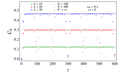
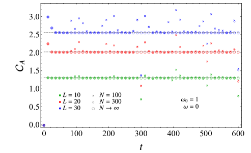
Figure 19: Temporal evolution of $\mathcal{C}_{A}$ after a global quantum quench with a gapless evolution Hamiltonian for a block $A$ made by $L$ consecutive sites adjacent to a boundary of harmonic chains with DBC made by $N$ sites. The data corresponding to $N\to\infty$ are obtained through a chain on the semi-infinite line. The horizontal dashed grey lines correspond to (5.26).

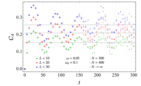
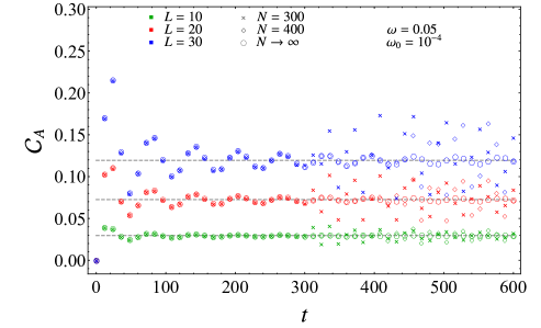
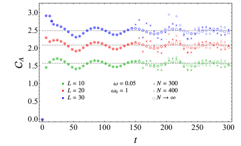
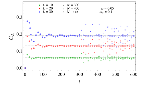
Figure 20: Temporal evolution of $\mathcal{C}_{A}$ after a global quantum quench with a gapped evolution Hamiltonian. In the left panels the chains are either on the circle or on the infinite line, while in the right panels the chains are either on the segment or on the semi-infinite line with DBC and $A$ is adjacent to a boundary. The dashed grey lines correspond to (5.26).

In this appendix we report further numerical results supporting (5.26) and (5.28).

In Fig. 19, Fig. 20. Fig. 21 and Fig. 23 we show some temporal evolutions of $\mathcal{C}_{A}$ for a block $A$ made by $L$ consecutive sites in harmonic chains with $N$ sites where $N$ is either finite or infinite, with the aim to check that (5.26) provides the correct asymptotic value as $t\to\infty$.

Each set of data corresponds to a choice of $N$, $L$, $\omega_{0}$ and $\omega$. The data represented by coloured markers have been found through (4.6), with the reduced correlators obtained either from (4.1) or from (4.1) when $N$ is finite (for PBC and DBC respectively) and either from (5.29) or from (5.30) when $N\to\infty$ (on the infinite line and on the semi-infinite line respectively). The horizontal dashed lines show the subregion complexity between the initial state and the GGE given by (5.26), obtained by reducing the correlators (A.31) and (A.34) for the target state and the correlators (5.29) and (5.30) at $t=0$ for the reference state (for the infinite line and the semi-infinite line respectively).

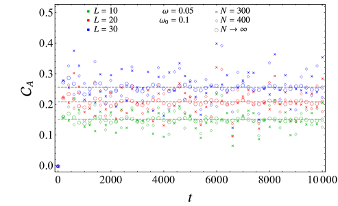
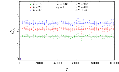
Figure 21: Temporal evolution of $\mathcal{C}_{A}$ after a global quantum quench with a gapped evolution Hamiltonian for a block made by $L$ consecutive sites in harmonic chains either with PBC or on the infinite line. The dashed grey lines correspond to (5.26).

In Fig. 19 we consider the temporal evolution of $\mathcal{C}_{A}$ when $\omega=0$, DBC are imposed and the block is adjacent to a boundary. The data obtained for finite $N$ are compared against the ones for $N\to\infty$, found for a block at the beginning of the semi-infinite chain. The main feature to highlight in these temporal evolutions are the plateaux occurring both for finite $N$ and for $N\to\infty$. The horizontal dashed lines in Fig. 19 correspond to the subregion complexity (5.26). These agreements support the assumption that the target state relaxes to an asymptotic state locally described by the GGE in (5.2) as $t\to\infty$. For a given set of parameters, the height of the plateaux is independent of $N$, while it increases as either $L$ or $\omega_{0}$ increases. Comparing the two panels of Fig. 19, where different values of $\omega_{0}$ are considered, one observes that the local maxima occur (when $N\to\infty$ there is only the first one) for large enough $\omega_{0}$. We also highlight the absence of oscillations in the formation of the plateaux when the evolution Hamiltonian is gapless.

In Fig. 20 and Fig. 21 the evolution Hamiltonians are gapped with $\omega=0.05$. We show data obtained for harmonic chains either with PBC or on the infinite line in the left panels and for harmonic chains either with DBC or on the semi-infinite line (with the block adjacent to a boundary) in the right panels. In these evolutions, data corresponding to the same $\omega$ and $\omega_{0}$ collapse for $t<N/2$ in the left panels and for $t<N$ in the right panels. The main difference with respect to the gapless evolutions in Fig. 19 are the oscillations after the initial growth around the asymptotic value, which is evaluated through (5.26) and corresponds to the horizontal dashed grey lines, whose height depends on $\omega$ and $\omega_{0}$. Fig. 21 highlights the fact that, for harmonic chains with PBC or on the infinite line, very long time is needed to reach the asymptotic value given by (5.26). Comparing the two panels in Fig. 21, one notices that the amplitude of the oscillations decreases as $|\omega-\omega_{0}|$ increases.

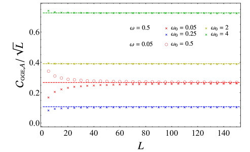
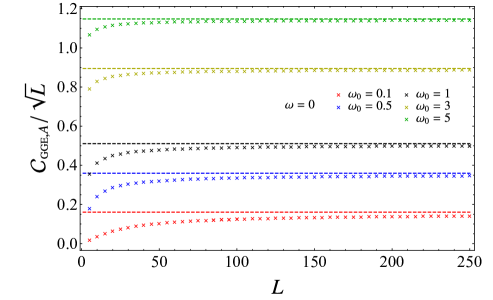
Figure 22: Asymptotic value of $\mathcal{C}_{\textrm{\tiny GGE},A}$ in (5.26) for a block made by $L$ consecutive sites which is either in the infinite chain (left panel) or adjacent to the origin of a semi-infinite chain with DBC (right panel). The horizontal dashed lines show $\mathcal{C}_{\textrm{\tiny GGE}}/\sqrt{N}$ as $N\to\infty$, from (5.24). These results support the last equality in (5.28).

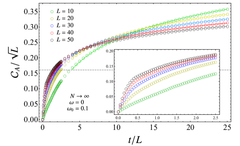
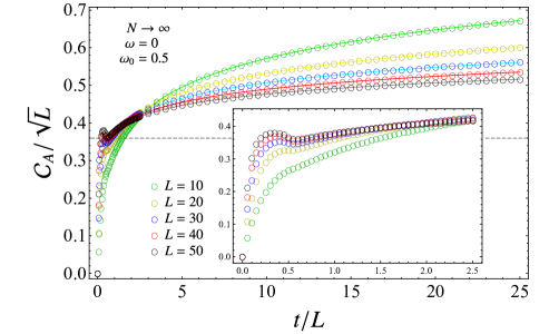
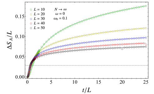
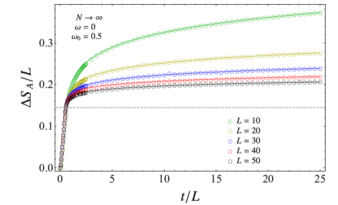
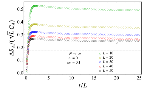
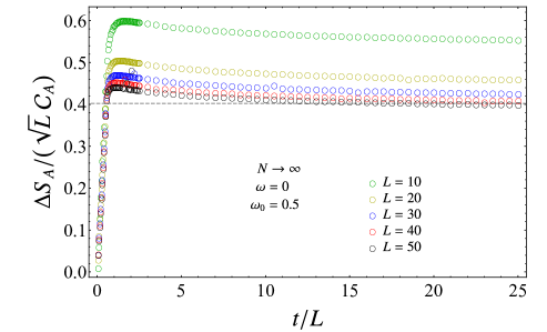
Figure 23: Temporal evolutions after a global quantum quench with a gapless evolution Hamiltonian and either $\omega_{0}=0.1$ (left panels) or $\omega_{0}=0.5$ (right panels) of $\mathcal{C}_{A}$ (top panels), of $\Delta S_{A}$ (middle panels) and of $\Delta S_{A}/\mathcal{C}_{A}$ (bottom panels) for a block made by $L$ consecutive sites in an infinite harmonic chain.

The numerical results in Fig. 22 provide the main outcome of this appendix. Since (5.24) tells us that $\mathcal{C}_{\textrm{\tiny GGE}}/\sqrt{N}$ is finite as $N\to\infty$ (see the left panel of Fig. 13) let us consider $\mathcal{C}_{\textrm{\tiny GGE},A}/\sqrt{L}$ in the limit $L\to\infty$, where $\mathcal{C}_{\textrm{\tiny GGE},A}$ is given by (5.26). The data reported in Fig. 22 for this quantity support the validity of the last equality in (5.28). The coloured data points have been obtained from (5.26), by employing the reduced correlators from (A.31) and (A.34) for the target state and the reduced correlators from (5.29) e (5.30) at $t=0$ for the reference state (like in Fig. 17 and Fig. 18). The horizontal dashed lines represent the asymptotic values obtained from (5.24), which depend only on $\omega_{0}$ and $\omega$. Comparing the two panels in Fig. 22, one realises that larger $L$’s are needed to reach the asymptotic value when the evolution Hamiltonian is gapless. Considering the red data points in the left panel of Fig. 22, notice that the asymptotic value (5.24) is symmetric under the exchange $\omega\leftrightarrow\omega_{0}$, as already remarked in the text above (5.24), while the sets of data points converging to it do not display this symmetry.

In Fig. 23 we consider harmonic chains on the infinite line and gapless evolution Hamiltonians. In particular, we study the temporal evolutions of $\mathcal{C}_{A}/\sqrt{L}$ (from (4.6)), of $\Delta S_{A}/L$ and of the ratio $\Delta S_{A}/(\sqrt{L}\,\mathcal{C}_{A})$ in terms of $t/L$, for various $L$’s and two values of $\omega_{0}$. The reduced covariance matrices have been obtained from the correlators (5.29). The growths of $\mathcal{C}_{A}$ and of $\Delta S_{A}$ from $t/L\simeq 7$ to $t/L\simeq 25$ have been fitted through the function $a\log(t/L)+b$ (coloured solid lines in Fig. 23), finding that the coefficient of the logarithmic term is positive and decreases as $L$ increases. In the top panels of Fig. 23, after the initial growth, $\mathcal{C}_{A}$ reaches a local maximum, then it decreases until $t/L\simeq 1/2$ and finally the curves follow the logarithmic growth mentioned above. This behaviour, which is more evident as $\omega_{0}$ increases, is highlighted in the insets. It would be interesting to explore higher value of $L$ in order to check whether, in the limit of $L\to\infty$, a saturation is observed to the value given by (5.24), which provides the horizontal dashed lines in the top panels of Fig. 23. The horizontal dashed lines in the middle panels are obtained from (5.16). In the bottom panels of Fig. 23, we show the temporal evolutions of the ratio $\Delta S_{A}/(\sqrt{L}\,\mathcal{C}_{A})$, which exhibit a mild logarithmic decreasing for large values of $t/L$. This tells us that the logarithmic growths of $\mathcal{C}_{A}$ and $\Delta S_{A}$ are very similar. However, the values of $L$ are not large enough to determine whether the numerical data points asymptote to a constant value as $t/L\to\infty$.

References

- [1] M. A. Nielsen, “A Geometric Approach to Quantum Circuit Lower Bounds”, Quantum Info. Comput. 6, 213–262 (2006), quant-ph/0502070.
- [2] M. A. Nielsen, M. R. Dowling, M. Gu and A. Doherty, “Quantum computation as geometry”, Science 311, 1133–1135 (2006), quant-ph/0603161.
- [3] M. R. Dowling and M. A. Nielsen, “The Geometry of Quantum Computation”, Quantum Info. Comput. 8, 861–899 (2008), quant-ph/0701004.
- [4] J. Watrous, “Quantum Computational Complexity”, Encyclopedia of Complexity and Systems Science , 7174 (2009), arxiv:0804.3401.
- [5] S. Aaronson, “The Complexity of Quantum States and Transformations: From Quantum Money to Black Holes”, arxiv:1607.05256.
- [6] D. Aharonov, A. Kitaev and N. Nisan, “Quantum Circuits with Mixed States”, quant-ph/9806029.
- [7] L. Susskind, “Computational Complexity and Black Hole Horizons”, Fortsch. Phys. 64, 24 (2016), arxiv:1403.5695.
- [8] L. Susskind and Y. Zhao, “Switchbacks and the Bridge to Nowhere”, arxiv:1408.2823.
- [9] D. A. Roberts, D. Stanford and L. Susskind, “Localized shocks”, JHEP 1503, 051 (2015), arxiv:1409.8180.
- [10] D. Stanford and L. Susskind, “Complexity and Shock Wave Geometries”, Phys. Rev. D 90, 126007 (2014), arxiv:1406.2678.
- [11] L. Susskind, “Entanglement is not enough”, Fortsch. Phys. 64, 49 (2016), arxiv:1411.0690.
- [12] M. Alishahiha, “Holographic Complexity”, Phys. Rev. D 92, 126009 (2015), arxiv:1509.06614.
- [13] A. R. Brown, D. A. Roberts, L. Susskind, B. Swingle and Y. Zhao, “Holographic Complexity Equals Bulk Action?”, Phys. Rev. Lett. 116, 191301 (2016), arxiv:1509.07876.
- [14] A. R. Brown, D. A. Roberts, L. Susskind, B. Swingle and Y. Zhao, “Complexity, action, and black holes”, Phys. Rev. D 93, 086006 (2016), arxiv:1512.04993.
- [15] J. L. Barbon and E. Rabinovici, “Holographic complexity and spacetime singularities”, JHEP 1601, 084 (2016), arxiv:1509.09291.
- [16] D. Carmi, R. C. Myers and P. Rath, “Comments on Holographic Complexity”, JHEP 1703, 118 (2017), arxiv:1612.00433.
- [17] R. Jefferson and R. C. Myers, “Circuit complexity in quantum field theory”, JHEP 1710, 107 (2017), arxiv:1707.08570.
- [18] S. Chapman, J. Eisert, L. Hackl, M. P. Heller, R. Jefferson, H. Marrochio and R. C. Myers, “Complexity and entanglement for thermofield double states”, SciPost Phys. 6, 034 (2019), arxiv:1810.05151.
- [19] M. Guo, J. Hernandez, R. C. Myers and S.-M. Ruan, “Circuit Complexity for Coherent States”, JHEP 1810, 011 (2018), arxiv:1807.07677.
- [20] L. Hackl and R. C. Myers, “Circuit complexity for free fermions”, JHEP 1807, 139 (2018), arxiv:1803.10638.
- [21] R. Khan, C. Krishnan and S. Sharma, “Circuit Complexity in Fermionic Field Theory”, Phys. Rev. D 98, 126001 (2018), arxiv:1801.07620.
- [22] P. Braccia, A. L. Cotrone and E. Tonni, “Complexity in the presence of a boundary”, JHEP 2002, 051 (2020), arxiv:1910.03489.
- [23] S. Chapman and H. Z. Chen, “Complexity for Charged Thermofield Double States”, arxiv:1910.07508.
- [24] M. Doroudiani, A. Naseh and R. Pirmoradian, “Complexity for Charged Thermofield Double States”, JHEP 2001, 120 (2020), arxiv:1910.08806.
- [25] M. Guo, Z.-Y. Fan, J. Jiang, X. Liu and B. Chen, “Circuit complexity for generalised coherent states in thermal field dynamics”, arxiv:2004.00344.
- [26] P. Caputa, N. Kundu, M. Miyaji, T. Takayanagi and K. Watanabe, “Anti-de Sitter Space from Optimization of Path Integrals in Conformal Field Theories”, Phys. Rev. Lett. 119, 071602 (2017), arxiv:1703.00456.
- [27] B. Czech, “Einstein Equations from Varying Complexity”, Phys. Rev. Lett. 120, 031601 (2018), arxiv:1706.00965.
- [28] P. Caputa, N. Kundu, M. Miyaji, T. Takayanagi and K. Watanabe, “Liouville Action as Path-Integral Complexity: From Continuous Tensor Networks to AdS/CFT”, JHEP 1711, 097 (2017), arxiv:1706.07056.
- [29] S. Chapman, M. P. Heller, H. Marrochio and F. Pastawski, “Toward a Definition of Complexity for Quantum Field Theory States”, Phys. Rev. Lett. 120, 121602 (2018), arxiv:1707.08582.
- [30] A. Bhattacharyya, P. Caputa, S. R. Das, N. Kundu, M. Miyaji and T. Takayanagi, “Path-Integral Complexity for Perturbed CFTs”, JHEP 1807, 086 (2018), arxiv:1804.01999.
- [31] P. Caputa and J. M. Magan, “Quantum Computation as Gravity”, Phys. Rev. Lett. 122, 231302 (2019), arxiv:1807.04422.
- [32] S. Chapman, D. Ge and G. Policastro, “Holographic Complexity for Defects Distinguishes Action from Volume”, JHEP 1905, 049 (2019), arxiv:1811.12549.
- [33] H. A. Camargo, M. P. Heller, R. Jefferson and J. Knaute, “Path integral optimization as circuit complexity”, Phys. Rev. Lett. 123, 011601 (2019), arxiv:1904.02713.
- [34] D. Ge and G. Policastro, “Circuit Complexity and 2D Bosonisation”, JHEP 1910, 276 (2019), arxiv:1904.03003.
- [35] Y. Sato and K. Watanabe, “Does Boundary Distinguish Complexities?”, JHEP 1911, 132 (2019), arxiv:1908.11094.
- [36] J. Erdmenger, M. Gerbershagen and A.-L. Weigel, “Complexity measures from geometric actions on Virasoro and Kac-Moody orbits”, arxiv:2004.03619.
- [37] M. Flory and M. P. Heller, “Complexity and Conformal Field Theory”, arxiv:2005.02415.
- [38] M. Flory and M. P. Heller, “Conformal field theory complexity from Euler-Arnold equations”, arxiv:2007.11555.
- [39] F. H. L. Essler and M. Fagotti, “Quench dynamics and relaxation in isolated integrable quantum spin chains”, J. Stat. Mech. 1606, 064002 (2016), arxiv:1603.06452.
- [40] P. Calabrese and J. Cardy, “Quantum quenches in 1 + 1 dimensional conformal field theories”, J. Stat. Mech. 1606, 064003 (2016), arxiv:1603.02889.
- [41] P. Calabrese and J. L. Cardy, “Evolution of entanglement entropy in one-dimensional systems”, J. Stat. Mech. 2005, P04010 (2005), cond-mat/0503393.
- [42] P. Calabrese and J. L. Cardy, “Time-dependence of correlation functions following a quantum quench”, Phys. Rev. Lett. 96, 136801 (2006), cond-mat/0601225.
- [43] P. Calabrese and J. Cardy, “Quantum Quenches in Extended Systems”, J. Stat. Mech. 0706, P06008 (2007), arxiv:0704.1880.
- [44] M. Rigol, V. Dunjko, V. Yurovsky and M. Olshanii, “Relaxation in a Completely Integrable Many-Body Quantum System: An Ab Initio Study of the Dynamics of the Highly Excited States of 1D Lattice Hard-Core Bosons”, Phys. Rev. Lett. 98, 050405 (2007), cond-mat/0604476.
- [45] E. Ilievski, J. De Nardis, B. Wouters, J.-S. Caux, F. H. L. Essler and T. Prosen, “Complete Generalized Gibbs Ensembles in an Interacting Theory”, Phys. Rev. Lett. 115, 157201 (2015), arxiv:1507.02993.
- [46] L. Vidmar and M. Rigol, “Generalized Gibbs ensemble in integrable lattice models”, J. Stat. Mech. 1606, 064007 (2016), arxiv:1604.03990.
- [47] D. W. Alves and G. Camilo, “Evolution of complexity following a quantum quench in free field theory”, JHEP 1806, 029 (2018), arxiv:1804.00107.
- [48] H. A. Camargo, P. Caputa, D. Das, M. P. Heller and R. Jefferson, “Complexity as a novel probe of quantum quenches: universal scalings and purifications”, Phys. Rev. Lett. 122, 081601 (2019), arxiv:1807.07075.
- [49] T. Ali, A. Bhattacharyya, S. Shajidul Haque, E. H. Kim and N. Moynihan, “Time Evolution of Complexity: A Critique of Three Methods”, JHEP 1904, 087 (2019), arxiv:1810.02734.
- [50] J. Jiang, J. Shan and J. Yang, “Circuit complexity for free Fermion with a mass quench”, Nucl. Phys. B 954, 114988 (2020), arxiv:1810.00537.
- [51] M. Moosa, “Evolution of Complexity Following a Global Quench”, JHEP 1803, 031 (2018), arxiv:1711.02668.
- [52] S. Chapman, H. Marrochio and R. C. Myers, “Holographic complexity in Vaidya spacetimes. Part I”, JHEP 1806, 046 (2018), arxiv:1804.07410.
- [53] S. Chapman, H. Marrochio and R. C. Myers, “Holographic complexity in Vaidya spacetimes. Part II”, JHEP 1806, 114 (2018), arxiv:1805.07262.
- [54] J. Eisert, M. Cramer and M. Plenio, “Area laws for the entanglement entropy - a review”, Rev. Mod. Phys. 82, 277 (2010), arxiv:0808.3773.
- [55] H. Casini and M. Huerta, “Entanglement entropy in free quantum field theory”, J. Phys. A 42, 504007 (2009), arxiv:0905.2562.
- [56] P. Calabrese and J. Cardy, “Entanglement entropy and conformal field theory”, J. Phys. A 42, 504005 (2009), arxiv:0905.4013.
- [57] I. Peschel and V. Eisler, “Reduced density matrices and entanglement entropy in free lattice models”, J. Phys. A 42, 504003 (2009), arxiv:0906.1663.
- [58] M. Rangamani and T. Takayanagi, “Holographic Entanglement Entropy”, Springer (2017).
- [59] M. Headrick, “Lectures on entanglement entropy in field theory and holography”, arxiv:1907.08126.
- [60] E. Tonni, “An Introduction to Entanglement Measures in Conformal Field Theories and AdS/CFT”, Springer Proc. Phys. 239, 69 (2020).
- [61] S. Sotiriadis and J. Cardy, “Quantum quench in interacting field theory: A Self-consistent approximation”, Phys. Rev. B 81, 134305 (2010), arxiv:1002.0167.
- [62] J. S. Cotler, M. P. Hertzberg, M. Mezei and M. T. Mueller, “Entanglement Growth after a Global Quench in Free Scalar Field Theory”, JHEP 1611, 166 (2016), arxiv:1609.00872.
- [63] V. Alba and P. Calabrese, “Entanglement dynamics after quantum quenches in generic integrable systems”, SciPost Physics 4, 17 (2018), arxiv:1712.07529.
- [64] V. E. Hubeny, M. Rangamani and T. Takayanagi, “A Covariant holographic entanglement entropy proposal”, JHEP 0707, 062 (2007), arxiv:0705.0016.
- [65] J. Abajo-Arrastia, J. Aparicio and E. Lopez, “Holographic Evolution of Entanglement Entropy”, JHEP 1011, 149 (2010), arxiv:1006.4090.
- [66] J. Cardy and E. Tonni, “Entanglement hamiltonians in two-dimensional conformal field theory”, J. Stat. Mech. 1612, 123103 (2016), arxiv:1608.01283.
- [67] G. Di Giulio, R. Arias and E. Tonni, “Entanglement hamiltonians in 1D free lattice models after a global quantum quench”, J. Stat. Mech. 1912, 123103 (2019), arxiv:1905.01144.
- [68] J. Surace, L. Tagliacozzo and E. Tonni, “Operator content of entanglement spectra in the transverse field Ising chain after global quenches”, Phys. Rev. B 101, 241107(R) (2020), arxiv:1909.07381.
- [69] X. Wen, S. Ryu and A. W. W. Ludwig, “Entanglement hamiltonian evolution during thermalization in conformal field theory”, J. Stat. Mech. 1811, 113103 (2018), arxiv:1807.04440.
- [70] A. Coser, E. Tonni and P. Calabrese, “Entanglement negativity after a global quantum quench”, J. Stat. Mech. 1412, P12017 (2014), arxiv:1410.0900.
- [71] Y. Chen and G. Vidal, “Entanglement contour”, J. Stat. Mech. 2014, P10011 (2014), arxiv:1406.1471.
- [72] A. Coser, C. De Nobili and E. Tonni, “A contour for the entanglement entropies in harmonic lattices”, J. Phys. A 50, 314001 (2017), arxiv:1701.08427.
- [73] E. Caceres, S. Chapman, J. D. Couch, J. P. Hernandez, R. C. Myers and S.-M. Ruan, “Complexity of Mixed States in QFT and Holography”, JHEP 2003, 012 (2020), arxiv:1909.10557.
- [74] G. Di Giulio and E. Tonni, “Complexity of mixed Gaussian states from Fisher information geometry”, JHEP 2012, 101 (2020), arxiv:2006.00921.
- [75] S.-M. Ruan, “Purification Complexity without Purifications”, arxiv:2006.01088.
- [76] H. A. Camargo, L. Hackl, M. P. Heller, A. Jahn, T. Takayanagi and B. Windt, “Entanglement and Complexity of Purification in (1+1)-dimensional free Conformal Field Theories”, arxiv:2009.11881.
- [77] C. A. Agón, M. Headrick and B. Swingle, “Subsystem Complexity and Holography”, JHEP 1902, 145 (2019), arxiv:1804.01561.
- [78] C. Rao, “Information and the accuracy attainable in the estimation of statistical parameters”, Bull. Calcutta Math. Soc. 37, 81 (1945).
- [79] C. Atkinson and A. Mitchell, “Rao’s Distance Measure”, Sankhyā: The Indian Journal of Statistics 43, 345 (1981).
- [80] S. Amari, “Information Geometry and Its Applications”, Springer (2016).
- [81] R. Abt, J. Erdmenger, M. Gerbershagen, C. M. Melby-Thompson and C. Northe, “Holographic Subregion Complexity from Kinematic Space”, JHEP 1901, 012 (2019), arxiv:1805.10298.
- [82] M. Alishahiha, K. Babaei Velni and M. R. Mohammadi Mozaffar, “Black hole subregion action and complexity”, Phys. Rev. D 99, 126016 (2019), arxiv:1809.06031.
- [83] R. Auzzi, S. Baiguera, A. Legramandi, G. Nardelli, P. Roy and N. Zenoni, “On subregion action complexity in AdS3 and in the BTZ black hole”, JHEP 2001, 066 (2020), arxiv:1910.00526.
- [84] B. Chen, W.-M. Li, R.-Q. Yang, C.-Y. Zhang and S.-J. Zhang, “Holographic subregion complexity under a thermal quench”, JHEP 1807, 034 (2018), arxiv:1803.06680.
- [85] R. Auzzi, G. Nardelli, F. I. Schaposnik Massolo, G. Tallarita and N. Zenoni, “On volume subregion complexity in Vaidya spacetime”, JHEP 1911, 098 (2019), arxiv:1908.10832.
- [86] Y. Ling, Y. Liu, C. Niu, Y. Xiao and C.-Y. Zhang, “Holographic Subregion Complexity in General Vaidya Geometry”, JHEP 1911, 039 (2019), arxiv:1908.06432.
- [87] Y.-T. Zhou, X.-M. Kuang, Y.-Z. Li and J.-P. Wu, “Holographic subregion complexity under a thermal quench in an Einstein-Maxwell-axion theory with momentum relaxation”, Phys. Rev. D 101, 106024 (2020), arxiv:1912.03479.
- [88] S. Ryu and T. Takayanagi, “Holographic derivation of entanglement entropy from AdS/CFT”, Phys. Rev. Lett. 96, 181602 (2006), hep-th/0603001.
- [89] M. Headrick and T. Takayanagi, “A Holographic proof of the strong subadditivity of entanglement entropy”, Phys. Rev. D 76, 106013 (2007), arxiv:0704.3719.
- [90] E. Tonni, “Holographic entanglement entropy: near horizon geometry and disconnected regions”, JHEP 1105, 004 (2011), arxiv:1011.0166.
- [91] V. E. Hubeny, H. Maxfield, M. Rangamani and E. Tonni, “Holographic entanglement plateaux”, JHEP 1308, 092 (2013), arxiv:1306.4004.
- [92] C. Weedbrook, S. Pirandola, R. García-Patrón, N. J. Cerf, T. C. Ralph, J. H. Shapiro and S. Lloyd, “Gaussian quantum information”, Rev. Mod. Phys. 84, 621 (2012), arxiv:1110.3234.
- [93] G. Adesso, S. Ragy and A. R. Lee, “Continuous Variable Quantum Information: Gaussian States and Beyond”, Open Systems and Information Dynamics 21, 1440001 (2014), arxiv:1401.4679.
- [94] A. Serafini, “Quantum Continuous Variables: A Primer of Theoretical Methods”, CRC Press (2017).
- [95] R. Bhatia, “Positive Definite Matrices”, Princeton University Press (2007).
- [96] J. Williamson, “On the Algebraic Problem Concerning the Normal Forms of Linear Dynamical Systems”, American Journal of Mathematics 58, 141 (1936).
- [97] J. Cardy, “Thermalization and Revivals after a Quantum Quench in Conformal Field Theory”, Phys. Rev. Lett. 112, 220401 (2014), arxiv:1403.3040.
- [98] V. Kac and P. Cheung, “Quantum Calculus”, Springer (2002).
- [99] V. Balasubramanian, A. Bernamonti, J. de Boer, N. Copland, B. Craps, E. Keski-Vakkuri, B. Muller, A. Schafer, M. Shigemori and W. Staessens, “Holographic Thermalization”, Phys. Rev. D 84, 026010 (2011), arxiv:1103.2683.
- [100] V. Balasubramanian, A. Bernamonti, N. Copland, B. Craps and F. Galli, “Thermalization of mutual and tripartite information in strongly coupled two dimensional conformal field theories”, Phys. Rev. D 84, 105017 (2011), arxiv:1110.0488.
- [101] A. Allais and E. Tonni, “Holographic evolution of the mutual information”, JHEP 1201, 102 (2012), arxiv:1110.1607.
- [102] R. Callan, J.-Y. He and M. Headrick, “Strong subadditivity and the covariant holographic entanglement entropy formula”, JHEP 1206, 081 (2012), arxiv:1204.2309.
- [103] V. E. Hubeny, M. Rangamani and E. Tonni, “Thermalization of Causal Holographic Information”, JHEP 1305, 136 (2013), arxiv:1302.0853.
- [104] V. E. Hubeny and H. Maxfield, “Holographic probes of collapsing black holes”, JHEP 1403, 097 (2014), arxiv:1312.6887.
- [105] Z.-Y. Fan and M. Guo, “Holographic complexity under a global quantum quench”, Nucl. Phys. B 950, 114818 (2020), arxiv:1811.01473.
- [106] I. Peschel, “Calculation of reduced density matrices from correlation functions”, J. Phys. A 36, L205 (2003), cond-mat/0212631.
- [107] K. Audenaert, J. Eisert, M. Plenio and R. Werner, “Entanglement Properties of the Harmonic Chain”, Phys. Rev. A 66, 042327 (2002), quant-ph/0205025.
- [108] M. Plenio, J. Eisert, J. Dreissig and M. Cramer, “Entropy, entanglement, and area: analytical results for harmonic lattice systems”, Phys. Rev. Lett. 94, 060503 (2005), quant-ph/0405142.
- [109] M. Cramer, J. Eisert, M. Plenio and J. Dreissig, “An Entanglement-area law for general bosonic harmonic lattice systems”, Phys. Rev. A 73, 012309 (2006), quant-ph/0505092.
- [110] M. G. Nezhadhaghighi and M. A. Rajabpour, “Entanglement dynamics in short- and long-range harmonic oscillators”, Phys. Rev. B 90, 205438 (2014), arxiv:1408.3744.
- [111] L. Hackl, E. Bianchi, R. Modak and M. Rigol, “Entanglement production in bosonic systems: Linear and logarithmic growth”, Phys. Rev. A 97, 032321 (2018), arxiv:1710.04279.
- [112] H. Liu and S. J. Suh, “Entanglement growth during thermalization in holographic systems”, Phys. Rev. D 89, 066012 (2014), arxiv:1311.1200.
- [113] R. G. Unanyan and M. Fleischhauer, “Entanglement dynamics in harmonic-oscillator chains”, Phys. Rev. A 89, 062330 (2014), arxiv:1011.4838.
- [114] T. Barthel and U. Schollwock, “Dephasing and the Steady State in Quantum Many-Particle Systems”, Phys. Rev. Lett. 100, 100601 (2008), arxiv:0711.4896.
- [115] M. Cramer, C. Dawson, J. Eisert and T. Osborne, “Exact Relaxation in a Class of Nonequilibrium Quantum Lattice Systems”, Phys. Rev. Lett. 100, 030602 (2008), cond-mat/0703314.
- [116] M. Cramer and J. Eisert, “A quantum central limit theorem for non-equilibrium systems: exact local relaxation of correlated states”, New J. Phys. 12, 055020 (2010), arxiv:0911.2475.
- [117] S. Sotiriadis and P. Calabrese, “Validity of the GGE for quantum quenches from interacting to noninteracting models”, J. Stat. Mech. 1407, P07024 (2014), arxiv:1403.7431.
- [118] T. P. E. Ilievski, M. Medenjak and L. Zadnik, “Quasilocal charges in integrable lattice systems”, J. Stat. Mech. 1606, 064008 (2016), arxiv:1603.00440.
- [119] P. Calabrese, “Entanglement spreading in non-equilibrium integrable systems”, arxiv:2008.11080, in: “Les Houches Summer School: Integrability in Atomic and Condensed Matter Physics”.
- [120] M. Fagotti and F. H. L. Essler, “Reduced density matrix after a quantum quench”, Physical Review B 87, 245107 (2013), arxiv:1302.6944.
- [121] S. R. Das, D. A. Galante and R. C. Myers, “Universal scaling in fast quantum quenches in conformal field theories”, Phys. Rev. Lett. 112, 171601 (2014), arxiv:1401.0560.
- [122] P. Caputa, S. R. Das, M. Nozaki and A. Tomiya, “Quantum Quench and Scaling of Entanglement Entropy”, Phys. Lett. B 772, 53 (2017), arxiv:1702.04359.
- [123] V. Eisler and I. Peschel, “Evolution of entanglement after a local quench”, J. Stat. Mech. 2007, P06005 (2007), cond-mat/0703379.
- [124] P. Calabrese and J. Cardy, “Entanglement and correlation functions following a local quench: a conformal field theory approach”, J. Stat. Mech. 0710, P10004 (2007), arxiv:0708.3750.
- [125] D. S. Ageev, I. Y. Aref’eva, A. A. Bagrov and M. I. Katsnelson, “Holographic local quench and effective complexity”, JHEP 1808, 071 (2018), arxiv:1803.11162.
- [126] D. Ageev, “Holographic complexity of local quench at finite temperature”, Phys. Rev. D 100, 126005 (2019), arxiv:1902.03632.
- [127] V. Eisler and I. Peschel, “Analytical results for the entanglement Hamiltonian of a free-fermion chain”, J. Phys. A 50, 284003 (2017), arxiv:1703.08126.
- [128] V. Eisler and I. Peschel, “Properties of the entanglement Hamiltonian for finite free-fermion chains”, J. Stat. Mech. 1810, 104001 (2018), arxiv:1805.00078.
- [129] E. Tonni, J. Rodríguez-Laguna and G. Sierra, “Entanglement hamiltonian and entanglement contour in inhomogeneous 1D critical systems”, J. Stat. Mech. 1804, 043105 (2018), arxiv:1712.03557.
- [130] V. Eisler, E. Tonni and I. Peschel, “On the continuum limit of the entanglement Hamiltonian”, J. Stat. Mech. 1907, 073101 (2019), arxiv:1902.04474.
- [131] G. Di Giulio and E. Tonni, “On entanglement hamiltonians of an interval in massless harmonic chains”, J. Stat. Mech. 2003, 033102 (2020), arxiv:1911.07188.
- [132] V. Eisler, G. Di Giulio, E. Tonni and I. Peschel, “Entanglement Hamiltonians for non-critical quantum chains”, J. Stat. Mech. 2010, 103102 (2020), arxiv:2007.01804.