On the computational and statistical complexity of over-parameterized matrix sensing
| Jiacheng Zhuo† | Jeongyeol Kwon♭ | Nhat Ho⋄ | Constantine Caramanis♭ |
| Department of Computer Science, University of Texas at Austin†, |
| Department of Electrical and Computer Engineering, University of Texas at Austin♭ |
| Department of Statistics and Data Sciences, University of Texas at Austin⋄ |
Abstract
We consider solving the low rank matrix sensing problem with Factorized Gradient Descend (FGD) method when the true rank is unknown and over-specified, which we refer to as over-parameterized matrix sensing. If the ground truth signal is of rank , but we try to recover it using where and , the existing statistical analysis falls short, due to a flat local curvature of the loss function around the global maxima. By decomposing the factorized matrix into separate column spaces to capture the effect of extra ranks, we show that converges to a statistical error of after number of iterations where is the output of FGD after iterations, is the variance of the observation noise, is the -th largest eigenvalue of , and is the number of sample. Our results, therefore, offer a comprehensive picture of the statistical and computational complexity of FGD for the over-parameterized matrix sensing problem.
1 Introduction
We consider the low rank matrix sensing problem: we are given i.i.d. observations from the data generating model , where is a symmetric random sensing matrix, is the target rank symmetric matrix we want to recover, and is a zero-mean sub-Gaussian noise with variance proxy . The low rank matrix sensing problem has found applications in various scenarios, such as multi-task regression, vector auto-regressive process, image processing, metric embedding, quantum tomography, and so on [Candes and Plan, 2011, Negahban and Wainwright, 2011, Recht et al., 2010, Jain et al., 2013, Gross et al., 2010, Candès et al., 2011, Waters et al., 2011, Kalev et al., 2015]. One common approach to recover a low-rank matrix is to solve the following optimization problem:
| (1) |
where is a chosen rank based on domain knowledge of the data. This problem can be solved by relaxing the rank constraint to nuclear norm constraint [Recht et al., 2010, Candes and Plan, 2011]. However for computational benefits, it is common to reformulate this as a non-convex problem by introducing such that and solving the transformed problem [Bhojanapalli et al., 2016a, Chen and Wainwright, 2015, Jain et al., 2013, Hardt, 2014]
| (2) |
Solving this formulation directly with gradient descent method on the matrix is usually referred to as the Factorized Gradient Descent (FGD) method, which is given by:
| (3) |
where is the step size and denotes the gradient evaluated at iteration with i.i.d. samples.
When the specified rank matches the ground truth rank , namely, the true rank is known, FGD converges linearly to a statistical error [Chen and Wainwright, 2015], and the statistical error is minimax optimal up to log factors [Candes and Plan, 2011]. However, in the real world applications, it is often a big challenge to correctly identify the true rank , and hence the practitioners tend to over-specify the rank. When the rank is over-specified (i.e. ), we refer to that setting as the over-parameterized matrix sensing problem.
The over-parameterized matrix sensing comes with many challenges, and to the best of our knowledge, none of the existing works offer a complete understanding about the computational and statistical performance of FGD under this setting.
First and foremost, we are faced a degenerate Hessian around the global maxima caused by the over-specification of the rank.
Hence previous works with known rank settings [Bhojanapalli et al., 2016a, Zheng and Lafferty, 2016, Tu et al., 2016] are no longer applicable since they rely on local strong convexity around the global maxima.
The analysis of Chen and Wainwright [2015] is also void, because with over-parameterization the ratio of the first and the -th eigenvalue of is infinity.
Li et al. [2018] focus on the implicit regularization effect with early stopping, and their analysis is limited to the setting where there is no observation noise (), and they can only guarantee recovery within a lower and upper bounded iteration range (as in their Theorem 1).
In summary, despite the current progress on the matrix sensing problem, the following questions remain unclear:
If we solve the over-parameterized matrix sensing problem with FGD, (1) what is the achievable statistical error? (2) and how fast we can recover a target matrix ?
Contribution. This paper offers a comprehensive analysis of over-parameterized low-rank matrix sensing with the FGD method. We show that converges to a final statistical error of after number of iterations where and respectively the -th largest eigenvalue of and the standard deviation of the observation noise. It is different from the computational and statistical behavior of FGD when the true rank is known, namely, the FGD converges to a radius of convergence around the true matrix after iterates [Chen and Wainwright, 2015] where is the largest eigenvalue of . Since we assume no a priori knowledge of true rank , the statistical error is also minimax optimal up to logarithmic factors [Candes and Plan, 2011]. Furthermore, the number of iterations is needed in the over-parameterized setting as the local curvature of the loss function (1) around the global maxima is not quadratic and therefore the FGD only converges sub-linearly to the global maxima; see the simulations in Figure 1 for an illustration. Finally, when , i.e., in the noiseless case, we can guarantee the exact recovery similar to when we correctly specify the rank [Chen and Wainwright, 2015].
1.1 Related Work
Works related to Matrix Sensing.
Early works on matrix sensing often perform a semidefinite programming (SDP) relaxation, and replace the nonconvex rank constraint with a convex constraint based on the trace norm or nuclear norm; see for example [Candes and Plan, 2011, Recht et al., 2010, Negahban and Wainwright, 2011, Chen et al., 2013] and the references therein. Candes and Plan [2011] show that for any estimator based on observations, , where is the ground truth rank matrix that we want to recover, and is the standard deviation of the (sub)-Gaussian observation noise (see Section 1.4 for details). This convex relaxation approach is nearly optimal in this sense. Although we can theoretically solve this convex problem in polynomial time, the computational cost is often prohibitively high for large scale problems. For example, if we solve this SDP problem with the classical interior point method, the computational cost is roughly [Boyd et al., 2004, Chen and Wainwright, 2015] Although recently some tailored algorithms [Zheng and Lafferty, 2015, Tu et al., 2016] are developed to solve this convex problem, their computational complexity is at least since this SDP involves multiplication of two matrices in . This computational overhead motivates the study of FGD method. The low rank matrix sensing problem is tightly connected to the low rank matrix completion problem, since they have the same population update when solved by (factorized) gradient method, and they can often be analyzed by very similar techniques [Negahban and Wainwright, 2012, Koltchinskii et al., 2011, Chi et al., 2019].
Works related to FGD.
The idea of factorizing the low rank matrix dates back to Burer and Monteiro [2003, 2005]. Bhojanapalli et al. [2016a] characterize the computational convergence behavior of FGD method for general convex and strongly convex function using the restricted strong convexity argument. However, such analysis cannot be converted into statistical analysis. Chen and Wainwright [2015] offer a general theoretical framework for understanding FGD method from both computational and statistical perspective. Specifically, they show that with suitable initialization, FGD converges geometrically up to a statistical precision. However, their analysis only works when we know the ground truth rank ().
In this work we focus on local convergence as this is the crux in statistical analysis (see [Chen and Wainwright, 2015]). Initialization condition can be achieved via spectral methods (see [Bhojanapalli et al., 2016a, Tu et al., 2016, Zheng and Lafferty, 2016]). Moreover, the works by Bhojanapalli et al. [2016b], Ge et al. [2016], and Zhang et al. [2019] show that reformulation (2) does not have any spurious local minima from optimization’s perspective, indicating that it is possible to extend our analysis to random initialization.
Recently, Li et al. [2018] look into the implicit regularization effect in the learning of over-parameterized matrix factorization with FGD. They show that if there is no observation noise () and , FGD tends to first recover the majority part of the true signal (that is of rank ) due to the implicit regularization effect of the FGD method. However their analysis can only address the noiseless case, and can not be extended to the more realistic setting when the observation is noisy, i.e., . Moreover, they only guarantee recovery within an iteration lower bound and upper bound (e.g., as in the Theorem 1 in Li et al. [2018], the number of iterations to reach the target accuracy has an upper bound and lower bound), which is not in line with the common notion of convergence and statistical rate. We focus on the statistical rate, which means we want to understand the algorithm behavior if run the algorithm for infinitely long. (Further discussion can be found in Section 4).
Localized analysis for degenerate landscape.
When the curvature around the local optimum degenerates, first-order methods such as gradient descent slow down due to vanishing gradients as the estimator gets closer to the local optimum. This phenomenon is reported in various optimization problems with degenerate landscapes in weakly separated mixture of distributions [Dwivedi et al., 2020a, Kwon et al., 2020]. We can observe the same phenomenon when the rank is over-specified for low-rank matrix factorization problems.
The localization technique is a powerful analysis tool to handle degenerate landscapes with a tight statistical rate. This technique has been used widely in the empirical process theory literature [van der Vaart and Wellner, 2000]. We now see how the localization argument can be applied for a low-rank matrix sensing when we over-specify the rank. In result we obtain a tight statistical rate of FGD which matches the known information-theoretical lower bound for this problem even if we over-specify the rank.
1.2 Motivating Simulations
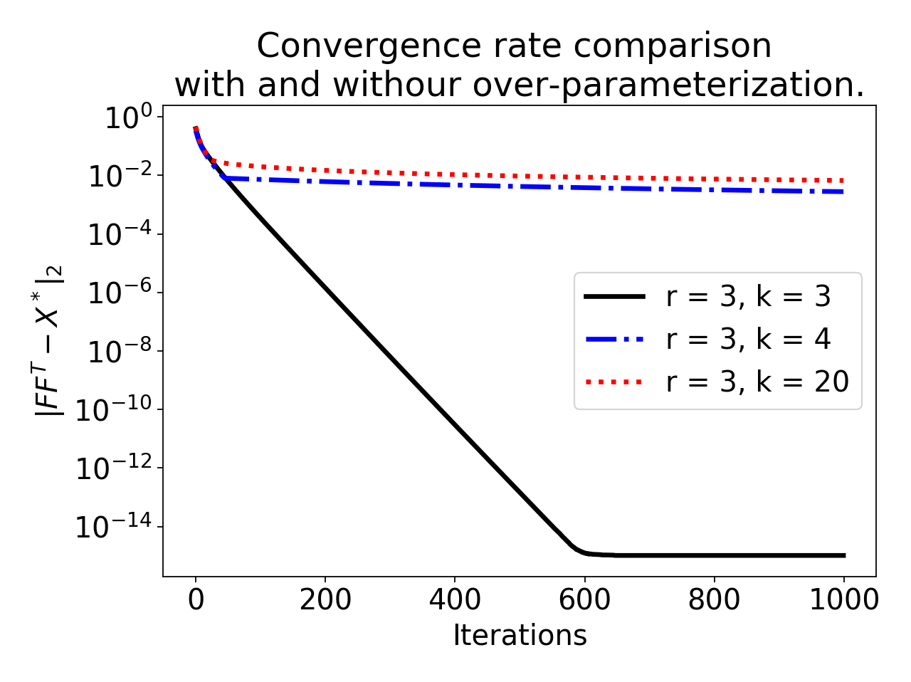
In the simulations, we consider the dimension , the true rank , and the number of samples . We first generate random orthonormal matrices and such that the union of their column spaces is . We set to be a diagonal matrix, with its entries be respectively, and zero elsewhere. Hence . The upper triangle entries of the sensing matrices are sampled from standard Gaussian distribution, and we fill the lower triangle entries accordingly such that are symmetric. We further assume that there is no observation noise, so that we have a better understanding of the convergence behavior of the algorithm.
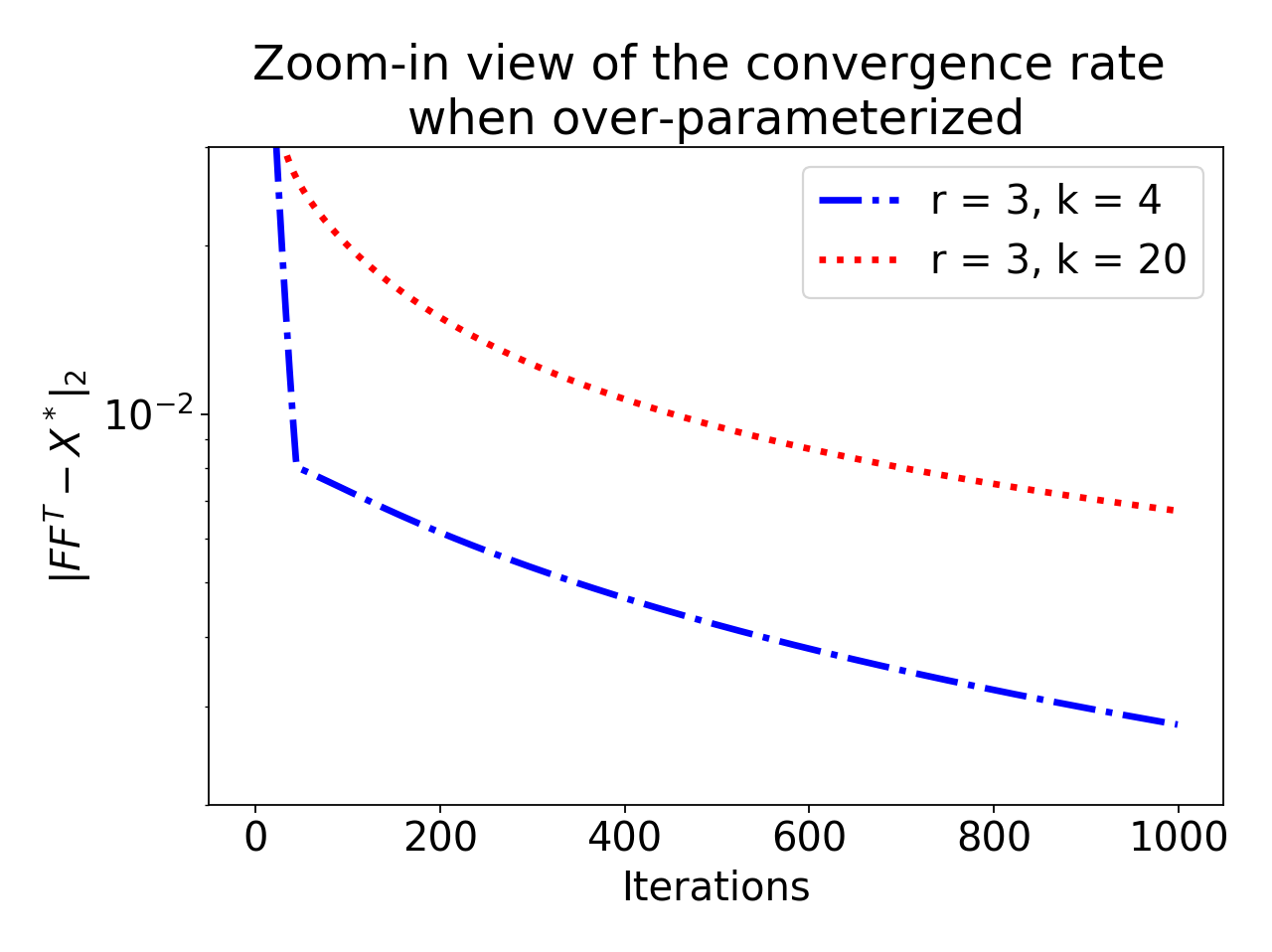
Let be the sequence generated by the FGD method as in equation (3) with . The simulation results are shown in Figure 1. When we correctly specify the rank (i.e. ), the FGD method converge geometrically towards machine precision. However, even if we increase the specified rank by , FGD will end up with a much slower convergence rate. A zoom-in view of the convergence rate shows that, FGD might first converge geometrically, and then converge sub-linearly. This phenomenon is not captured by the recent works about FGD [Li et al., 2018, Chen and Wainwright, 2015]. What exactly is the convergence rate? And what about the statistical error? These are the questions that we want to answer in this work.
1.3 Organization
The remainder of the paper is organized as follows. In Section 2, we present the convergence rate of the FGD iterates under the over-parameterized matrix sensing setting. Then, we present the proof sketch of the results in Section 3. The detailed proofs of the main results are deferred to the Appendices while we conclude the paper with a few discussions in Section 4.
1.4 Notations
In the paper, we use bold lower case letters to represent vectors, such as , and bold upper case letters to represent matrices, such as . When is a matrix, we use to represent the element on the -th row and -th column of , unless otherwise specified. We use for matrix inner product. For example . We denote as the smallest integer greater than or equal to for any . We write (respectively ) if is positive definite (respectively positive semidefinite) for square matrices and . We write to represent the sequence . We also use the short hand to represent We use and to denote the first eigenvalue and the -th eigenvalue of respectively, which is the ground truth rank matrix that we want to recover. And we use to denote the conditional number: .
We also use the standard asymptotic complexity notation. Specifically, implies for some constant and for large enough , implies for some constant and for large enough , and implies for some constant and for large enough . When factors are omitted, we use , , to represent , , respectively.
Definition 1.
(Sub-Gaussian Random Variable). We call a random variable with mean sub-Gaussian with variance proxy if , .
Definition 2.
(Sub-Gaussian Sensing Matrix). We call a matrix a sub-Gaussian sensing matrix if it is sampled as follow: each upper triangle entry () is sampled i.i.d. from a zero-mean sub-Gaussian distribution with variance proxy , each lower triangle entry () , and the diagonal entries are sample from i.i.d. from a zero-mean sub-Gaussian distribution with variance proxy .
2 Main Result
Before we present our main result, we formally introduce the decomposition notation for . Let the eigen-decomposition of (eigenvalues ordered by the absolute values) be given by
where , , , . Without loss of generality we assume that the both and are orthonormal and (i.e. and together span the entire ). Denote be the largest value in , be the smallest value in , and be the largest value in . Since we assume is of approximately rank , there is a non-trivial gap between and . In this section, we assume that . Since the union of the column space of and spans the entire , then for any , there exits matrices and such that
As goes to infinity, we hope that converges to , converges to , and and converges to zero, and hence converges to .
We introduce the decomposition and study the convergence of , , and separately. This decomposition technique is essential, since we can then bypass some technical difficulties when we over-specify the rank. For example we do not have to establish the uniqueness (up to rotational ambiguity) of the optimal solution as in the Lemma 1 in Chen and Wainwright [2015]. Moreover, this gives more insights about which part is the computational and/or statistical bottleneck. As we will see shortly (both in Theorem 1 and Lemma 3), it is the convergence of that slows down the entire process of the convergence. Similar decomposition technique is also employed in the work of Li et al. [2018].
Here we focus on the local convergence of FGD method within the following basin of attraction:
Assumption 1.
(Initialization assumption)
| (4) |
Note that is a universal constant and is chosen for the ease of presentation. Note that one can use spectrum method to achieve this initialization [Chen and Wainwright, 2015, Bhojanapalli et al., 2016a, Tu et al., 2016]. Connecting the initialization condition to our decomposition strategy, we need to control in our analysis. The following Lemma establish the connection between what we need in the analysis and Assumption 1.
Lemma 1.
If , then
Theorem 1.
(Main result) Assume the following settings: (1) ; (2) we have good initialization as in Assumption 1; (3) the sample size for some universal constant ; (4) the step size , (5) s are sub-Gaussian sensing matrices. Let be the sequence generated by the FGD algorithm as in Equation 3. Then, the following holds:
-
(a)
After steps, for some universal constant , where .
-
(b)
After steps, , and for some constants and , where .
(1) The sequences and first converge linearly and then sub-linearly. Theorem 1 indicates that the sequences and first converge linearly from to , and then converge sub-linearly to . Furthermore, the sequence always converges sublinearly towards . This is consistent with our simulations in Figure 2. As we will see later in Lemma 3, it is the convergence of that slows down the convergence of , and incurring the sublinear convergence of and .
(2) There is a convergence rate discrepancy between the population and finite-sample versions. It is often believed that the convergence rate is consistent even if we go from finite to infinitely large (i.e., from finite sample scenario to the scenario when we have access to the population gradient). However this is not the case in our setting. As we will show shortly in Lemma 2, if we have access to the population gradient, the convergence rates of the sequences and are linear all the way until zero. In our setting, going from population to finite-sample creates an unusual tangling factor, causing the convergence rate discrepancy between the finite-sample and population sequences.
(3) This achieves nearly minimax-optimal statistical error. At a glance the statistical error seems too good to be true compared to Yudong’s work, and even better than the minimax rate [Candes and Plan, 2011]. In fact the guarantees we offer are in spectral norm, while the typical rate in the related work is in Frobenius norm. Translating the spectral norm to Frobenius norm will introduce an extra factor. That is, the statistical error is if we evaluate . This statistical error is similar to the results in Chen and Wainwright [2015] when the rank is known, i.e., . Furthermore, we are able to cover both the noisy and noiseless matrix sensing settings. Given that we assume no a priori knowledge of true rank , the statistical error in Theorem 1 is minimax optimal up to log factors [Candes and Plan, 2011].
2.1 Simulation verification of the main result
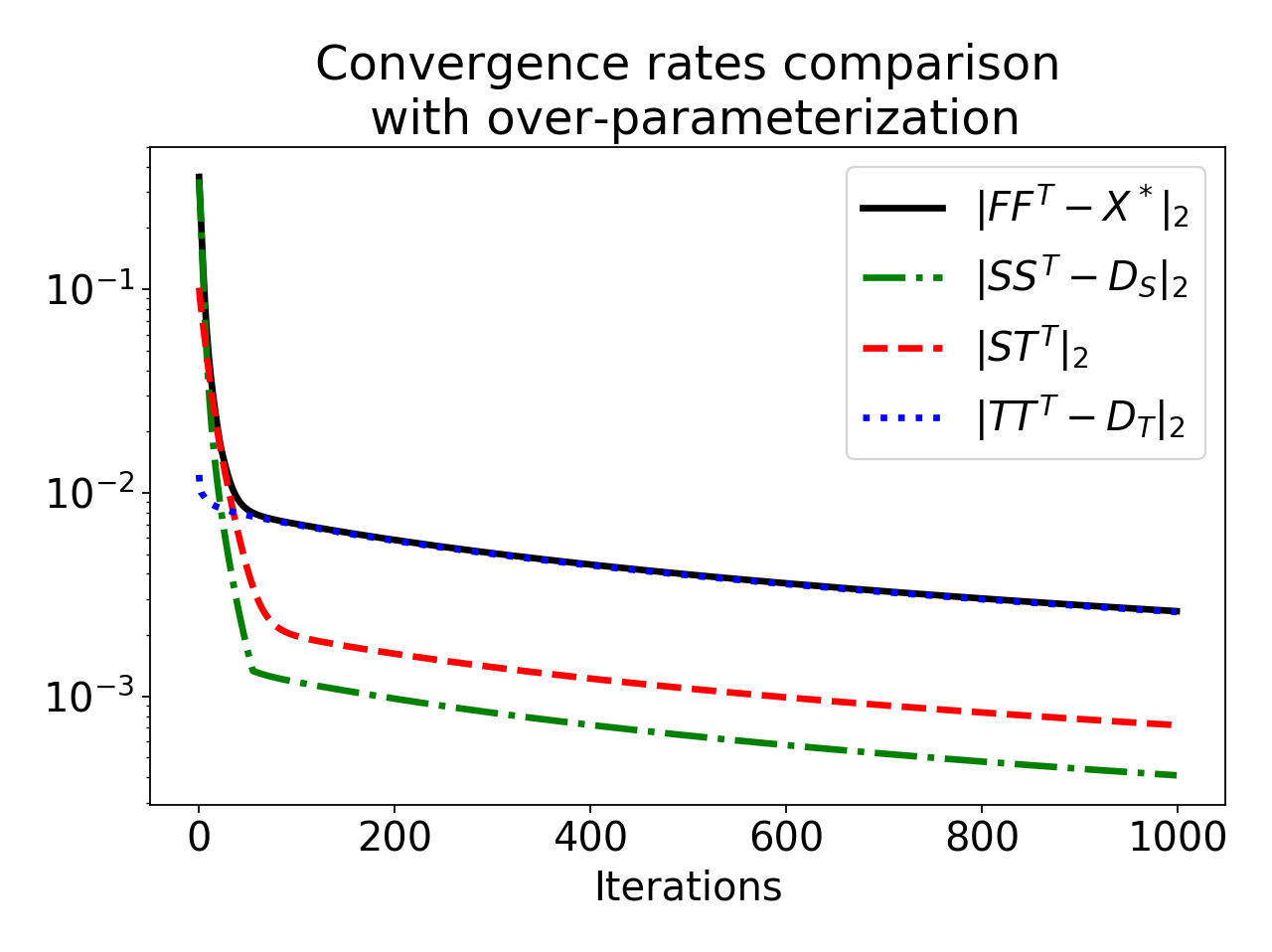
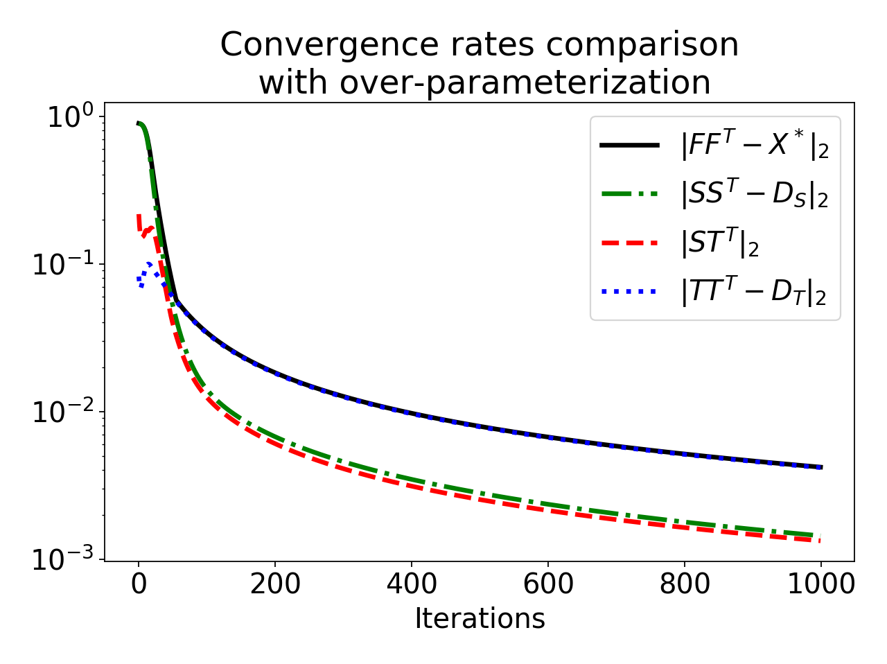
In this subsection we use the same simulation setup as in Section 1.2. Let be the sequence generated by the FGD method as in Equation 3, and let be defined as in the previous subsection.
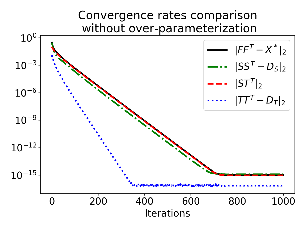
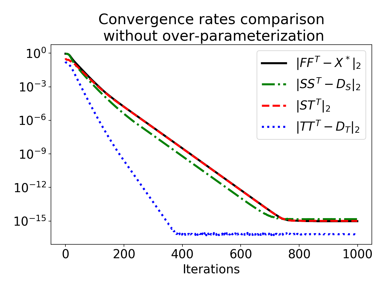
The simulation results are shown in Figure 2. In Figure 2(a), we plot , , , and against the algorithm iterations. The simulation results are aligned with our theory. As said in Theorem 1, and first converge linearly, and then sublinearly. Furthermore, is soon dominated by , which converges sub-linearly all the time. Note that these phenomena are when the true rank is and we set . If we correctly specify the rank (), the convergences will be linear, as shown in Figure 2(b). In Figures 2(c) and 2(d), we re-produce the result as in Figures 2(a) and 2(b) with random initialization. This indicates that our assumption of initialization could possibly be waived using recent insights about the global landscape of the matrix sensing problem [Zhang and Zhang, 2020].
3 Proof of the main result
The proof of the main result follows the typical population-sample analysis [Balakrishnan et al., 2017]. We first analyze the convergence behavior of the algorithm when we have access to the population gradient. Then in the finite sample setting, we quantify the difference between the population gradient and the finite sample gradient using concentration arguments, and use this difference plus the convergence result in population analysis, to characterize the convergence behavior in the finite sample setting.
While it is common to use the Restricted Isometric Property (RIP) as the building block to encapsulate the concentration requirement [Chen and Wainwright, 2015, Chi et al., 2019, Li et al., 2018], we build our results directly based on the concentration of sub-Gaussian sensing matrices for technical convenience. While it is possible to control the Frobenius norm directly, we find it technically easier and more reader friendly to show that the sequence converges, and the resulting statistical rate is tight. However, RIP is defined in Frobenius norm since it was first developed for vector and then extended to matrix [Recht et al., 2010, Candes and Plan, 2011]. Translating the Frobenius norm directly to spectral norm will incur a factor of sub-optimality. That being said, we believe that it is possible to establish similar results for directly, and hence we can use the general RIP notion. We leave this for future work.
3.1 Population analysis
The first step of our analysis is to understand the contraction if we have access to the population gradient. One can check that for any matrix with appropriate dimensions. Combined with the fact that , the population gradient (taking expectation over the observation noise and the observation matrices ) is
A closer look at the update in the Factored Gradient Method (Equation 3) with population gradient reveals that at each iteration, the update only changes the coefficient matrices and . Simple algebra using the last observation yields:
where we define the following operators:
Lemma 2.
(Contraction per iteration with access to the population gradient.) Set . We assume good initialization as in Assumption 1. Then we have:
-
(a)
,
-
(b)
,
-
(c)
,
-
(d)
.
According to Lemma 2 above, we have fast convergence in estimating , , but slow convergence in estimating . Intuitively, is slow because the local curvature of the population version of the loss function (2) is flat, namely, the Hessian matrix around the global maxima is degenerate. We know that when the curvature of the target matrix is undesirable, we can only guarantee sub-linear convergence rate [Bhojanapalli et al., 2016a].
3.2 Finite sample analysis
On top of our population analysis result, we consider the case when we only have access to the gradient evaluated with finitely many samples. Consider the deviation of the population and sample gradient:
We define to quantify this deviation:
and hence . If we can control , we can have contraction per-iteration, as shown in the lemma below. Note that we make no attempts to optimize the constants.
Lemma 3.
(Contraction per iteration.) Assume that we have the same setting as Theorem 1. Denote , and assume that is still sub-optimal to the statistical error: . Suppose
| (5) |
Then, we find that
| (6) | ||||
| (7) |
Moreover, denote . Then we have
| (8) |
Implication of equations (6) and (7):
Firstly, when goes to infinity, the sequence of has constant contraction at each step, and hence achieves a linear convergence after all. This matches our population results in Lemma 2. Secondly, if is finite, the sequence of still has constant contraction, until roughly the magnitude of reaches . This indicates that we will have a linear convergence behavior in the beginning, and then sublinear convergence, as is indicated in Theorem 1.
3.3 Proof sketch for the main theorem
In this subsection we offer a proof sketch for Theorem 1. Detailed proof can be found in Appendix B.2.
Lemma 3 is our key building block towards the main theorem. However there are two missing pieces. (1) Firstly we have to establish equation (5) so that Lemma 3 can be invoked for one iteration. (2) Secondly we have to find a way to correctly invoke Lemma 3 for all iterations and obtain the correct statistical rate.
We resolve the first point by bounding using matrix Bernstein concentration bound [Tropp, 2012] together with the -net discretization techniques.
Lemma 4.
Let be symmetric random matrices in , with the upper triangle entries () being independently sampled from an identical sub-Gaussian distribution whose mean is and variance proxy is . Let follows . Then
Lemma 5.
Let be a symmetric random matrix of dimension by . Its upper triangle entries () are independently sampled from an identical sub-Gaussian distribution whose mean is and variance proxy is . If is of rank and is in a bounded spectral norm ball of radius (i.e., ),
The proof of the above two concentration results can be found in the Appendix D. If we invoke these lemmas for , then we can immediately have
The linear convergence part.
Claim (a) in the main theorem is about linear convergence. We mention in the remark that equations (6) and (7) imply constant contractions for and respectively. To make the argument more precise, we consider . Then, we find that since . Also, by the choice of the constants in the lower bound of . Hence, when , we find that
The same arguments hold for . Therefore to obtain the linear convergence result as the part (a) in the main theorem, we can just invoke concentration lemmas for each iteration to obtain constant contraction, and then take union bound over all the iterations.
The sub-linear convergence part.
Claim (b) of the main theorem is about sublinear convergence, and is build upon equation (8).
Before we discuss how equation (5) holds in this sub-linear convergence case for all iteration , we briefly illustrate how equation (8) implies convergence to after iterations. By equation (8), we know that where . Hence
where inequality holds because is quadratic with respect to and we plug-in the optimal ; inequality holds because . Therefore, after number of iterations, .
We still need to show that equation (5) holds (with probability at least ) in this sub-linear convergence case for all iteration with high probability. To do so, we need to use the localization technique [Kwon et al., 2020, Dwivedi et al., 2020b, a]. Without the localization technique, the statistical error will be proportional to which is not tight. With the localization argument, we can improve it to , making the result nearly minimax optimal. We leave the details of this argument to Appendix B.2.
4 Discussion
In the paper, we provide a comprehensive analysis of the computational and statistical complexity of the Factorized Gradient Descent method under the over-parameterized matrix sensing problem, namely, when the true rank is unknown and over-specified. We show that converges to a minimax optimal radius of convergence after number of iterations where is the output of FGD after iterations. We now discuss a few natural questions with this work.
Can the results in Li et al. [2018] imply this work? We would like to explain the difference between our results and those in Li et al. [2018]. If we choose the specified rank as , we have the same problem setting, and use the same algorithm. However, the results are different. The key difference here is the sample complexity. As Li et al. [2018] focus on over-parameterization, their analysis requires samples, where is the rank of the ground truth matrix , while our analysis requires samples when . Since they only require samples, they cannot control the error of the over-parameterization part (equivalent to our part). In fact in their analysis, they only show that in a limited number of step, this error does not blow up. While with we can show that the over-parameterization part also converges, although with a slower convergence rate. Therefore, their results cannot imply ours.
Extensions to general convex function of low rank problem. One natural question to ask is, if our analysis can be extended to general convex function with respect to a low rank matrix. In particular, we consider minimizing a convex function , where is PSD. Let be the ground truth solution and it is of rank . We can as well reformulate our problem as minimizing where . Then as long as the population gradient with respect to is , and the sample gradients have good concentration around the population gradient, our analysis techniques should be applicable. For example, matrix completion and principle component analysis fall into this category [Chen and Wainwright, 2015]. However, extension the current results with over-parameterized matrix sensing to general convex function as in Chen and Wainwright [2015], or in Bhojanapalli et al. [2016a] would require more refined analysis. We leave this question for the future work.
5 Acknowledgements
We would like to thank Raaz Dwivedi, Koulik Khamaru, and Martin Wainwright for helpful discussion with this work.
Appendix A Proofs for population analysis
In this appendix, we provide all the proofs for population analysis of matrix sensing problem.
A.1 Proof of Lemma 2
We prove the four contraction results separately. To simplify the ensuing presentation, we drop all subscripts associated with the iteration counter.
Proof of the contraction result in Lemma 2:
We would like to prove the following inequality:
Indeed, from the formulation of , we have
We can group the terms in the RHS of the above equation according to whether they contain or not, namely, we find that
We first deal with the term. A direct application of inequality with operator norm leads to
From the choice of the step size and the initialization condition, the term is PSD matrix. Furthermore, for any , we have
where in step (i) we used , and by initialization condition and triangular inequality; step (ii) follows from choice of step size , and definition of the conditional number . Therefore, we arrive at the following inequality:
| (9) |
Proof of the contraction result in Lemma 2:
Recall that we want to demonstrate that
Firstly, from the formulations of and , we have the following equations:
| (11) |
Recall that, we have , and by initialization condition and triangular inequality, and we choose .
For the term in the first line of the RHS of equation (11) we have
For the term in the second line of the RHS of equation (11), direct calculation yields that
Lastly, for the second order term in the third line of the RHS of equation (11) we have
Plugging the above results into equation (11) leads to
Hence, we obtain the conclusion of claim (b) in Lemma 2.
Proof of the contraction result (c) in Lemma 2:
We would like to establish that
To check the convergence in low SNR, i.e., with small singular values, we assume that . It suggests that the focus is how fast converges to 0 when . Indeed, simple algebra indicates that
where we use the following shorthand notation:
We first bound the term. Inequalities with operator norm show that
Given these bounds, we find that
| (12) |
Now, we move to bound the term. Indeed, we have
| (13) |
Since is PSD, we can just relax this term to zero. Finally, we bound the term. Observe that,
since and . The remaining task is to bound . Let the singular value decomposition of as . Note that is a diagonal matrix with diagonal entries less than . We can proceed as
Since and , the above maximum is obtained at the largest singular value of . That is, we have
| (14) |
Now combining every pieces from equations (12), (13), and (14), we arrive at the following inequality:
As long as , the contraction rate is roughly . Therefore, we obtain the conclusion of claim (c) in Lemma 2.
Proof of the contraction result (d) in Lemma 2:
Direct calculation shows that
where we denote VI and VII as follows:
We first show that the . Firstly, since and the initialization condition , we have
Furthermore, by the choice of and the fact that , we find that
Putting these results together we have .
Now for the term, direct calculation shows that
Note that, since , , and , we obtain that
Collecting the above upper bounds with VI and VII, we arrive at
As a consequence, we reach the conclusion of claim (d) in Lemma 2.
A.2 Additional contraction results for population operators
In this appendix, we offer more population contraction (non-expansion) results, which are useful in showing the contraction results in finite sample setting.
Lemma 6.
Under the same settings as Lemma 2, we have
-
(a)
,
-
(b)
,
-
(c)
,
-
(d)
.
Proof.
With and simple algebraic manipulations, we obtain
Since by initialization condition and triangular inequality, we know that . Therefore, we obtain the conclusion of claim (a).
Move to claim (b), with simple algebraic manipulations, we can show that
By initialization condition and triangular inequality, we know that and , and hence . Hence, we reach the conclusion of claim (b).
With and direct calculation, we find that
By initialization condition and triangular inequality, we know that and , and hence . It leads to the conclusion of claim (c).
Finally, moving to claim (d), simple algebra shows that
By initialization condition and triangular inequality, we know that . As a consequence, we obtain the conclusion of claim (d).
∎
Appendix B Proofs for the finite sample analysis
Recall that, we denote as the population gradient at iteration and denote as the corresponding sample gradient with sample size :
Then, we can write our update as follows:
We assume the following decomposition by notations: . Therefore, we find that
| (15) |
where we define as follows:
Furthermore, direct calculation shows that
| (16) |
where is given by:
Similarly, we also have
| (17) |
Note that, in the above equations, and are the updates of the coefficients when we update and using the population gradient. Furthermore, , , and are second order terms and are relatively small. To facilitate the proof argument, we denote
We can see that is symmetric matrix, and
B.1 Proof for Lemma 3
Proof.
By Lemma 2 and Lemma 6, we have the following contraction results:
| (18) |
and the following non-expansion results:
| (19) |
For notation simplicity, let , and denote the statistical error . Since Assumption 1 is satisfied, and , we have by triangular inequality. Since by initialization, and , we have . Putting these results together, we have
| (20) |
For the ease of the presentation, we assign a value to the constant as in the number of sample . From the requirements of the lemma we know that We need to connect with for the development of the proof. Since and , by choosing , we have
| (21) |
Upper bound for :
According to equation (15), we have
where we can further expand and as follows:
and
Clearly, our target can be bounded by bounding the eight terms, marked from I to VIII. Note that the spectral norms of the terms (1) III and VI are the same, (2) IV and VII are the same, and (3)V and VIII are the same, which can be upper bounded as follows:
| III & VI: | |||
| IV & VII: | |||
| V & VIII: |
Lastly, consider the II term, we have the following bound:
| (22) |
where the last inequality holds by assuming . Putting all the above results together, we obtain that
where inequality is obtained by the non-expansion property of population update (cf. equations (19) and (20)) ; inequality is obtained by the fact that , and ; inequality is obtained by plugging in the relaxation of (cf. equation (5)) and organizing according to and .
Upper bound for :
According to equation (16), we have
where we can expand and as follows:
Clearly, our target upper bound for can be obtained by bounding the seven terms: I’ to VII’. Specifically, direct application of inequalities with operator norms leads to
Lastly, the II term is bounded as in Equation (22), namely, we have
Collecting the above results, we find that
where inequality is obtained by the non-expansion property of population update (cf. equations (19) and (20)); inequality is obtained by the fact that and . In summary, we have
| (26) |
With similar treatment as in , we have the following contraction result with respect to :
| (27) |
Given the above result, we can verify that
| (28) |
Upper bound for :
According to equation (17) and similar deductions as in previous bounds for and , we have
where the following expansions hold:
Given the formulations of the terms -, we find that
Assume that for . Note that, is not necessarily a constant. For notation simplicity we use the short hand that . With the choice of and equation (5), we have . Therefore, we obtain that
where inequality is obtained by the non-expansion property of population update (cf. equations (19) and (20)) and the assumption on (cf. equation (5)). For inequality , observe that the above quantity is a quadratic formula with respect to , and the maximum is taken when . Hence we can just safely plug-in . Now, we arrange by organizing according to and and obtain that
where inequality is obtained by , and inequality is obtained by organizing according to and .
For notation simplicity we introduce , and hence where . With some algebraic manipulations, we have
Furthermore, from equations (25) and (28), we have
Putting all these results together yields that
This completes the proof of the Lemma 3. ∎ In the lemma above we use to demonstrate how sample iteration conerges to population iteration as increases. However we do not need when is extremely large such that . This will lead to a waste of sample and lead to sub-optimal sample complexity result. Hence we introduce the following corollary in order to deal with the scenario .
Corollary 1.
Consider under the same setting and using the same notation as Lemma 3. Suppose Then
Moreover, denote . Then we have
| (29) |
Proof.
Note that Lemma 3 is established for . To complete the proof of our main theorem, we want to make sure that do not expand too much after we reaches the statistical accuracy.
Lemma 7.
Consider the same setting as Lemma 3, except that . We claim that .
Proof.
The proof of this Lemma is a simple extension using the proof of Lemma 3. As in the proof of Lemma 3, we know that
From the hypothesis, . Hence, we have
Similarly for , we have
Finally, for , we find that
where inequality (1) is deducted in the proof of Lemma 3; inequality (2) is by relaxing term I using Equation (18), relaxing , and grouping all other terms; inequality (3) is by the assumption that ; inequality (4) is by the choice of such that .
Putting all the results together, we obtain the conclusion of Lemma 7. ∎
B.2 Proof of Theorem 1
Our proof is divided into verifying claim (a) and claim (b).
Proof for claim (a) with the linear convergence:
From the result of Lemma 3, we know that
We consider . Note that . Then and by the choice of the constants in the lower bound of . Hence, when , we find that
| (30) |
We now have constant contraction for one iteration. We can invoke the Lemma 10 for once, Lemma 12 for iterations, and take the union bounds, to quantify the probability that equation (5) holds for all iteration . Shortly we will show that this probability is at least for some universal constant . But first we need to know how large we need the number of iterations to be. Suppose equation (5) holds for all iteration , then
where the final inequality holds by simply plugging in the initialization condition. After at most iterations, . Since , we further simplify this to . As a consequence, we claim that after iterations, for some universal constant .
Now the remaining task is to show that equation (5) holds for all iteration with probability at least . If is not too large, i.e. for some constant , then we invoke equation 35 in Lemma 12 for iterations. This holds with probability at least for some universal constant , since . If is large, i.e., for some universal constant , then we use Corollary 1 to establish equation (30), and we invoke equation (36) in Lemma 12 for iterations. This holds with probability at least for some universal constant , since .
Therefore equation (5) holds with probability at least for all iteration , and we complete our proof with .
With the same argument, we also obtain after iterations. Therefore, we obtain the conclusion of claim (a) in Theorem 1.
Proof for claim (b) with the sub-linear convergence:
For the sublinear convergence part in claim (b), we prove it by induction. We consider the base case. Since , we have by choosing . Therefore the base case is correct by the definitions of and .
The key induction step is proven in the Lemma 3, as the equation (8). However, as the convergence rate is sub-linear ultimately, it is sub-optimal to directly invoke concentration result (Lemma 12) to establish equation (5) at each iteration and take union bound over all the iterations. Hence, we adapt the standard localization techniques from empirical process theory to sharpen the rates. Note that, these techniques had also been used to study the convergence rates of optimization algorithms in mixture models settings [Dwivedi et al., 2020a, Kwon et al., 2020].
The key idea of the localization technique is that, instead of invoking the concentration result at each iteration, we only do so when is decreased by . More precisely, we divide all the iterations into epochs, where -th epoch starts at iteration , ends at iteration , and . We invoke Lemma 13 at to establish equation (5) for all the iterations in -th epoch. Finally, we take a union bound over all the epochs.
By definition, we have
From Lemma 10, we know that with probability at least ,
We only have to invoke this concentration result once for the entire algorithm analysis.
At iteration , note that . By Lemma 13 we know that, with probability at least , we have
Therefore, we find that
and equation (5) is satisfied at iteration . For notation simplicity, we define . Invoking Lemma 3, we have
where the last inequality just comes from . At iteration , by induction , and . Furthermore, we also have . Therefore, the following bounds hold:
Hence, equation (5) is satisfied for all iteration . Invoking Lemma 3, we have
with probability at least for a universal constant . This directly implies that
| (31) |
We first assume that equation (31) holds for all iterations , and then show that this is true with probability at least for some constant . With this, we claim that . To see this, we have
where inequality holds because is quadratic with respect to and we plug-in the optimal ; inequality holds because .
Therefore, after number of iterations, , which indicates that
| (32) |
Now what is left to be shown is that equation (31) holds for all iterations with probability at least for some constant . We first consider . If is not too large, i.e., for some constant , then we invoke equation (35) in Lemma 12 for iterations. This holds with probability at least for some universal constant , since . If is large, i.e., for some universal constant , then we use Corollary 1 to establish equation (31), and we invoke equation (36) in Lemma 12 for iterations. This holds with probability at least for some universal constant , since . If , we can show using above argument that after number of iterations equation (32) holds. After this, by Lemma 7 we know that . Then, we can invoke Lemma 3 or Corollary 1 without further invoking the concentration argument anymore, since the radius in the uniform concentration result does not change .
Appendix C Supporting Lemma
In this appendix, we provide proofs for supporting lemmas in the main text.
C.1 Proof of Lemma 1
Proof.
From the definition of operator norm, we have
Since is an orthonormal matrix, for any , we can find a vector such that . Hence, we find that
Without loss of generality we can write any as , such that for some , and for some since and are perpendicular to each other and they together span . If then is zero. It is because if , one can decrease to zero and increase to , which does make the target quantity smaller. Therefore, we have
where the final inequality is due to the Assumption 1. The same techniques can be applied to obtain
For , we claim that the following equations hold:
To see the last equality, let be the largest eigen-value (in magnitude) of and let be the corresponding eigen-vector. For some , let such that for some , for some , and and . Then, direct algebra leads to
For the RHS of the above equation, the optimal choice of is . We already know that the largest eigen-value (in magnitude) of is also . Therefore, we obtain that
Collecting the above results, we have . Then, an application of triangular inequality yields that
We can check that by decomposing the eigen-vector as above. Therefore, .
As a consequence, we obtain the conclusion of the lemma. ∎
Appendix D Concentration bounds
In this appendix, we want establish the uniform concentration bound for the following term:
for any matrix such that for some radius . To do so, we have to bound the spectral norm of each random observation, and then take Bernstein/Chernoff type bound.
Lemma 8.
(Matrix Bernstein, Theorem 1.4 in Tropp [2012]) Consider a finite sequence of independent, random, self-adjoint matrices with dimension . Assume that each random matrix satisfies
Then, for all ,
| (33) |
Lemma 9.
Let be a symmetric random matrix in , with the upper triangle entries () being independently sampled from an identical sub-Gaussian distribution whose mean is and variance proxy is . Let follows . Then
Proof.
Lemma 10.
(Lemma 4 re-stated) Let be symmetric random matrices in , with the upper triangle entries () being independently sampled from an identical sub-Gaussian distribution whose mean is and variance proxy is . Let follows . Then
Proof.
We prove the lemma by applying the matrix Bernstein bound. In fact, direct calculation shows that
Hence, we obtain
From the matrix Bernstein bound [Wainwright, 2019], we find that
For any , let . Then, the above bound becomes
Or equivalently, for any , let ,
As a consequence, we reach the conclusion of the lemma. ∎
Lemma 11.
Let be a symmetric random matrix in , with the upper triangle entries () being independently sampled from an identical sub-Gaussian distribution whose mean is and variance proxy is . Let be a deterministic symmetric matrix of the same dimension. Then, for some universal constant , we have
Proof.
We show this by standard -net argument. In particular, we have
Note that is sub-Gaussian with variance proxy , and is sub-Gaussian with variance proxy . Therefore and . By the union bound,
Since , we have
| (34) |
By the standard -net argument, let be the covering of . Then, we find that
Now we fix to be . Then, for equation (34) we take union bound over and we have
and . By choosing for reasonably large universal constant we have
As a consequence, we obtain the conclusion of the lemma.
∎
Lemma 12.
Let be a symmetric random matrix of dimension by , with the upper triangle entries () being independently sampled from an identical sub-Gaussian distribution whose mean is and variance proxy is . Let be a deterministic symmetric matrix of the same dimension. Then as long as for some universal , we have
| (35) |
Moreover when is larger than the order of , that is, if there exists a constant such that for some universal constant we have
| (36) |
Proof.
Following Lemma 8, we want to first bound the second order moment of the random matrices. Since and has no randomness, we have
The entry of equals to
For diagonal entries, i.e., , the expectation is not zero if and only if . Hence for diagonal entry , its expectation is
For off diagonal entries, i.e., , the expectation is not zero for that entry when (1) and , or when (2) and . For both cases, the expectation equals the entry of . Therefore, we obtain that
Hence the entry of equals when , and equals when . Hence and
Then, the following inequality holds:
where is a universal constant inherited from Lemma 11 and
Let , and as long as for some universal constant , we have
Hence we finish the proof for equation 35.
For the tightness of our statistical analysis, we need to consider the case when is larger than the order of polynomial of . If there exists a constant such that
then plugging in , we have
In summary, we reach the conclusion of the lemma. ∎
Lemma 13.
(Lemma 5 re-stated) Let be a symmetric random matrix of dimension by . Its upper triangle entries () are independently sampled from an identical sub-Gaussian distribution whose mean is and variance proxy is . If is of rank and is in a bounded spectral norm ball of radius (i.e. ), then we have
| (37) |
Moreover when is larger than the order of , that is, if there exists a constant such that for some universal constant we have
| (38) |
Proof.
To show this uniform convergence result, we use the standard discretization techniques (i.e. -net). In particular, we have
Since the above quantity is symmetric, we can take off the absolute value and only look at the one-side deviation. The crux is how to construct the -net for . We decompose . Since is of rank and , we can write where are vectors, with and for . Therefore
Now we can construct a standard -net for each , and in total we construct such epsilon net for . Hence we invoke equation (35) in Lemma 12 for -net on these norm balls: and take an union bound, we have
Similarly if we invoke the equation (36) for -net on these norm balls: and take an union bound, we also have
As a consequence, the conclusion of the lemma follows. ∎
References
- Balakrishnan et al. [2017] S. Balakrishnan, M. J. Wainwright, and B. Yu. Statistical guarantees for the EM algorithm: From population to sample-based analysis. Annals of Statistics, 45:77–120, 2017.
- Bhojanapalli et al. [2016a] S. Bhojanapalli, A. Kyrillidis, and S. Sanghavi. Dropping convexity for faster semi-definite optimization. In Conference on Learning Theory, pages 530–582, 2016a.
- Bhojanapalli et al. [2016b] S. Bhojanapalli, B. Neyshabur, and N. Srebro. Global optimality of local search for low rank matrix recovery. arXiv preprint arXiv:1605.07221, 2016b.
- Boyd et al. [2004] S. Boyd, S. P. Boyd, and L. Vandenberghe. Convex optimization. Cambridge university press, 2004.
- Burer and Monteiro [2003] S. Burer and R. D. Monteiro. A nonlinear programming algorithm for solving semidefinite programs via low-rank factorization. Mathematical Programming, 95(2):329–357, 2003.
- Burer and Monteiro [2005] S. Burer and R. D. Monteiro. Local minima and convergence in low-rank semidefinite programming. Mathematical Programming, 103(3):427–444, 2005.
- Candes and Plan [2011] E. J. Candes and Y. Plan. Tight oracle inequalities for low-rank matrix recovery from a minimal number of noisy random measurements. IEEE Transactions on Information Theory, 57(4):2342–2359, 2011.
- Candès et al. [2011] E. J. Candès, X. Li, Y. Ma, and J. Wright. Robust principal component analysis? Journal of the ACM (JACM), 58(3):1–37, 2011.
- Chen and Wainwright [2015] Y. Chen and M. J. Wainwright. Fast low-rank estimation by projected gradient descent: General statistical and algorithmic guarantees. arXiv preprint arXiv:1509.03025, 2015.
- Chen et al. [2013] Y. Chen, A. Jalali, S. Sanghavi, and C. Caramanis. Low-rank matrix recovery from errors and erasures. IEEE Transactions on Information Theory, 59(7):4324–4337, 2013.
- Chi et al. [2019] Y. Chi, Y. M. Lu, and Y. Chen. Nonconvex optimization meets low-rank matrix factorization: An overview. IEEE Transactions on Signal Processing, 67(20):5239–5269, 2019.
- Dwivedi et al. [2020a] R. Dwivedi, N. Ho, K. Khamaru, M. J. Wainwright, M. I. Jordan, and B. Yu. Singularity, misspecification, and the convergence rate of EM. Annals of Statistics, 48:3161–3182, 2020a.
- Dwivedi et al. [2020b] R. Dwivedi, N. Ho, K. Khamaru, M. J. Wainwright, M. I. Jordan, and B. Yu. Sharp analysis of Expectation-Maximization for weakly identifiable models. In AISTATS, 2020b.
- Ge et al. [2016] R. Ge, J. D. Lee, and T. Ma. Matrix completion has no spurious local minimum. In Advances in Neural Information Processing Systems, pages 2973–2981, 2016.
- Gross et al. [2010] D. Gross, Y.-K. Liu, S. T. Flammia, S. Becker, and J. Eisert. Quantum state tomography via compressed sensing. Physical review letters, 105(15):150401, 2010.
- Hardt [2014] M. Hardt. Understanding alternating minimization for matrix completion. In 2014 IEEE 55th Annual Symposium on Foundations of Computer Science, pages 651–660. IEEE, 2014.
- Jain et al. [2013] P. Jain, P. Netrapalli, and S. Sanghavi. Low-rank matrix completion using alternating minimization. In Proceedings of the forty-fifth annual ACM symposium on Theory of computing, pages 665–674, 2013.
- Kalev et al. [2015] A. Kalev, R. L. Kosut, and I. H. Deutsch. Quantum tomography protocols with positivity are compressed sensing protocols. npj Quantum Information, 1(1):1–6, 2015.
- Koltchinskii et al. [2011] V. Koltchinskii, K. Lounici, A. B. Tsybakov, et al. Nuclear-norm penalization and optimal rates for noisy low-rank matrix completion. The Annals of Statistics, 39(5):2302–2329, 2011.
- Kwon et al. [2020] J. Kwon, N. Ho, and C. Caramanis. On the minimax optimality of the EM algorithm for learning two-component mixed linear regression. arXiv preprint arXiv:2006.02601, 2020.
- Li et al. [2018] Y. Li, T. Ma, and H. Zhang. Algorithmic regularization in over-parameterized matrix sensing and neural networks with quadratic activations. In Conference On Learning Theory, pages 2–47. PMLR, 2018.
- Negahban and Wainwright [2011] S. Negahban and M. J. Wainwright. Estimation of (near) low-rank matrices with noise and high-dimensional scaling. The Annals of Statistics, pages 1069–1097, 2011.
- Negahban and Wainwright [2012] S. Negahban and M. J. Wainwright. Restricted strong convexity and weighted matrix completion: Optimal bounds with noise. The Journal of Machine Learning Research, 13(1):1665–1697, 2012.
- Recht et al. [2010] B. Recht, M. Fazel, and P. A. Parrilo. Guaranteed minimum-rank solutions of linear matrix equations via nuclear norm minimization. SIAM review, 52(3):471–501, 2010.
- Tropp [2012] J. A. Tropp. User-friendly tail bounds for sums of random matrices. Foundations of computational mathematics, 12(4):389–434, 2012.
- Tu et al. [2016] S. Tu, R. Boczar, M. Simchowitz, M. Soltanolkotabi, and B. Recht. Low-rank solutions of linear matrix equations via procrustes flow. In International Conference on Machine Learning, pages 964–973. PMLR, 2016.
- van der Vaart and Wellner [2000] A. W. van der Vaart and J. A. Wellner. Weak Convergence and Empirical Processes: With Applications to Statistics. Springer-Verlag, New York, NY, 2000.
- Vershynin [2018] R. Vershynin. High Dimensional Probability. An Introduction with Applications in Data Science. Cambridge University Press, 2018.
- Wainwright [2019] M. J. Wainwright. High-Dimensional Statistics: A Non-Asymptotic Viewpoint. Cambridge University Press, 2019.
- Waters et al. [2011] A. E. Waters, A. C. Sankaranarayanan, and R. Baraniuk. Sparcs: Recovering low-rank and sparse matrices from compressive measurements. In Advances in neural information processing systems, pages 1089–1097, 2011.
- Zhang and Zhang [2020] J. Zhang and R. Zhang. How many samples is a good initial point worth in low-rank matrix recovery? Advances in Neural Information Processing Systems, 33, 2020.
- Zhang et al. [2019] R. Y. Zhang, S. Sojoudi, and J. Lavaei. Sharp restricted isometry bounds for the inexistence of spurious local minima in nonconvex matrix recovery. Journal of Machine Learning Research, 20:1–34, 2019.
- Zheng and Lafferty [2015] Q. Zheng and J. Lafferty. A convergent gradient descent algorithm for rank minimization and semidefinite programming from random linear measurements. Advances in Neural Information Processing Systems, 28:109–117, 2015.
- Zheng and Lafferty [2016] Q. Zheng and J. Lafferty. Convergence analysis for rectangular matrix completion using Burer-Monteiro factorization and gradient descent. arXiv preprint arXiv:1605.07051, 2016.