A limit theorem for Bernoulli convolutions
and the -variation of functions in the Takagi class
Abstract
We consider a probabilistic approach to compute the Wiener–Young -variation of fractal functions in the Takagi class. Here, the -variation is understood as a generalization of the quadratic variation or, more generally, the variation of a trajectory computed along the sequence of dyadic partitions of the unit interval. The functions we consider form a very wide class of functions that are regularly varying at zero. Moreover, for each such function , our results provide in a straightforward manner a large and tractable class of functions that have nontrivial and linear -variation. As a corollary, we also construct stochastic processes whose sample paths have nontrivial, deterministic, and linear -variation for each function from our class. The proof of our main result relies on a limit theorem for certain sums of Bernoulli random variables that converge to an infinite Bernoulli convolution.
Key words: Wiener–Young –variation, Takagi class, pathwise Itô calculus, infinite Bernoulli convolution, central limit theorem, stochastic process with prescribed -variation
MSC 2020: 60F25, 28A80, 26A12, 60H05
1 Introduction
Probabilistic models of continuous random trajectories typically rely on solutions to stochastic differential equations or, more generally, on continuous semimartingales. The huge success of those models is in no small part due to the fact that they can be analyzed by means of Itô calculus. Itô calculus is however not restricted to the sample paths of a semimartingale: Föllmer [8] showed that every continuous function that admits a continuous quadratic variation along a fixed refining sequence of partitions can be used as an integrator for Itô integration and that a corresponding Itô formula holds. As shown in [10, 20, 24], this includes many functions previously studied in fractal analysis and geometry.
Cont and Perkowski [4] recently extended Föllmer’s pathwise Itô formula to integrators with higher than quadratic variation, the so-called variation. While quadratic variation is based on the squared increments of a function, variation is based on the power of the increments, where . In the realm of stochastic processes, the sample paths of fractional Brownian motion with Hurst index constitute the best-known class of such trajectories. At the same time, recent applications, such as the theory of rough volatility models based on the seminal paper [11] by Gatheral et al., have intensified the interest in creating new models for “rough” phenomena beyond the case of quadratic variation. Also in this strand of literature, the focus has so far been on models with finite and nontrivial variation.
From a mathematical point of view, however, there is no reason why attention should be restricted to variation based on power functions. A natural and much broader concept is given by the notion of -variation in the Wiener–Young sense. Here, for a function , the -variation of a continuous function along the dyadic partitions is given by
| (1.1) |
provided that the limit exists for all . Yet, most authors still focus exclusively on the case of power variation. Notable exceptions are the paper [18] by Marcus and Rosen, in which the -variation of Gaussian processes with stationary increments and local times of symmetric Lévy processes is obtained, and Kôno [16]. Note that the -variation along a fixed refining sequence of partitions as defined in (1.1) typically differs from the -variation defined as a supremum taken over all finite partitions. For Gaussian processes, the latter concept was studied, e.g., by Taylor [27] for and by Kawada and Kôno [15] for more general functions .
In this paper, we use a probabilistic approach to explore a class of fractal trajectories that admit the -variation for functions of the form
| (1.2) |
where and is any regularly varying function444 Recall that a measurable and strictly positive function , which is defined on some interval , is called regularly varying (at infinity) with index if as for all . If , the function is also called slowly varying. Throughout this paper, we will always assume that all regularly varying functions are defined on . This assumption can be made without loss of generality, as one can always consider the function . . In doing so, we address several high-level issues. First, we illustrate that finite and nontrivial power variation, which has so far been the default paradigm for characterizing the roughness of trajectories, appears to be the exception rather than the rule. In particular, one should expect -variation rather than power variation when studying continuous trajectories that do not arise as sample paths of a semimartingale. Second, for every function of the form (1.2), we construct explicit examples of trajectories with finite linear -variation along the dyadic partitions. These examples can be used in further analyses involving “rough” trajectories. Moreover, the idea underlying our construction of functions with prescribed -variation can probably be extended to more flexible models and into the realm of stochastic processes.
The class of functions we consider here belong to the so-called Takagi class, which was introduced by Hata and Yamaguti [14] and motivated by Takagi’s [26] celebrated example of a continuous nowhere differentiable function. This class was chosen due to its richness and tractability and also because it is closely related to the Wiener–Lévy construction of Brownian motion. The Takagi class consists of all functions that admit an expansion of the form
| (1.3) |
where is the tent map and is a sequence of real numbers for which the series converges absolutely. The special choice for some yields the class of so-called Takagi–Landsberg functions, which, for and , have finite nontrivial and linear variation as shown in [21]. For it is well known that is of finite total variation. The borderline case corresponds to the classical Takagi function, which is nowhere differentiable and hence not of finite total variation, even though . Instead, for , the function has linear -variation, , for , as shown by the authors in [13]. Note that this function is a special case of (1.2). Our method also extends to an even richer class of functions for which each scaled phase of the tent map in (1.3) is multiplied with an arbitrary sign (see (3.7) for details). This latter class can be fitted to empirical time series and gives also rise to a class of stochastic processes if the signs are chosen randomly.
Our approach to the -variation of functions in the Takagi class depends on the parameter in (1.2). For , our argument extends the approach via the central limit theorem for the Rademacher functions in the Faber–Schauder development of as presented in [13]. For , however, a new limit theorem is needed, which might be of independent interest. If is a sequence of real numbers and is an i.i.d. sequence of symmetric Bernoulli random variables, we investigate the limit of the “convolutions”
We show that if there exist , , and a slowly varying function such that
| (1.4) |
then
| (1.5) |
Note that the law of the limiting random variable is a scaled version of the infinite Bernoulli convolution with parameter . In Section 2, we will present an extended version of this result in which the are neither required to be independent nor identically distributed. This approach to the -variation via the condition (1.4) and the limiting result (1.5) is to some extent motivated by Gladyshev’s theorem [12] (see also the book [19] by Marcus and Rosen for a comprehensive survey). It extends previous work in [21, 25, 13].
The paper is structured as follows. In Section 2, we derive the convergence result (1.5) and the central limit theorem that will be needed for our results on the -variation of functions in the Takagi class. Our main result on this topic, Theorem 3.3, is stated in Section 3. The proof of Theorem 3.3 is given in Section 4.
2 A limit theorem for Bernoulli-type convolutions
For some , let be a sequence of random variables in , where is a given probability space. We assume for simplicity that the -norms of are uniformly bounded. Let furthermore be a sequence of real numbers and consider the random variables
We are first concerned with the limit of
as . Our corresponding result uses the concept of a slowly varying function, which was recalled in the footnote on page 4.
Theorem 2.1.
Suppose that for all and that there exist , , and a slowly varying function such that
| (2.1) |
Then
Proof of Theorem 2.1.
For , denote
where is chosen such that the arguments of the square roots are always positive. Thus,
| (2.2) |
Let be given. We first choose such that
| (2.3) |
Then we choose such that
| (2.4) |
Finally, we choose such that
| (2.5) |
Given this , we use (2.1) to pick such that
| (2.6) |
Hence,
| (2.7) |
Since is slowly varying, we can choose such that
Combining this with (2.2), we see that the left-hand side of (2.7) is strictly positive for . Hence, we may take square roots to get
| (2.8) |
for all . Moreover, with (2.6) we get that for ,
Similarly, we conclude a corresponding lower bound and obtain that for ,
| (2.9) |
The Potter bounds (see, e.g., Theorem 1.5.6 in [3]) yield that there is such that for ,
With (2.9), we obtain that for ,
| (2.10) |
Note that
By Minkowski’s inequality and with ,
| (2.11) |
To deal with the first sum on the right-hand side, we use (2.5) and (2.10) to get that for ,
In the same way, we get the lower bound
Using (2.4) and (2.3), we thus get the following estimate for the first sum on the right-hand side of (2.11)
where . For the right-most sum in (2.11), we have
| (2.12) |
We will show below that our assumptions imply that . Therefore, the right-hand side of (2.12) can be made smaller than by choosing sufficiently large. Thus, we see that the -distance between and is smaller than if is sufficiently large.
Now we briefly discuss the case where in (2.1). In that case, we are typically in the regime of the central limit theorem. This is suggested, for instance, by [28], where a central limit theorem for reversible Markov chains was obtained under the condition that the variance, , satisfies for a slowly varying function . Since is regularly varying with index , we see that, in our situation, this condition is a special case of condition (3.4) with . In the following proposition, we formulate implications between stronger and weaker versions of condition (2.1) with .
Now we are going to formulate a simple central limit theorem in the form needed in the next section. We believe that this result is well known but were unable to find an exact reference to the literature. Due to the large number of existing variants of the central limit theorem, we confine ourselves here to the basic case that will actually be needed in Section 4.
Lemma 2.2.
Suppose that is an i.i.d. sequence of symmetric -valued Bernoulli random variables such that as . Then, for every , the laws of converge in the -Wasserstein metric to the standard normal distribution.
Proof. As , it then follows that
It is hence easy to see that the sequence satisfies Lindeberg’s condition, which yields that converges in law to . Thus, to conclude convergence in the -Wasserstein metric, it is sufficient to show that is uniformly bounded in for some ; this follows, e.g., from Lemma 5.61 and Corollary A.50 in [9]. We actually show a stronger condition, namely that is uniformly bounded for all . Since , we can drop the absolute value in the exponent. Then,
3 -variation of functions in the Takagi class
In this section, we will apply the limit theorems from Section 2 to the problem of computing the -variation of functions in the Takagi class. To this end, let be a function with . The -variation of a continuous function along the sequence of dyadic partitions is defined as
provided that the limit exists for all . Due to the uniform continuity of , we may, without loss of generality, restrict to the domain . For and , we obtain the total variation of . For , we obtain the usual quadratic variation, and for with the variation. Here, we are interested in functions for which the correct may not be of the form but rather has a more complex structure.
Let denote the tent map. The Takagi class, as introduced by Hata and Yamaguti [14], consists of all functions that admit an expansion of the form
| (3.1) |
where is a sequence of real numbers for which the series converges absolutely. Clearly, the series on the right-hand side of (3.1) converges uniformly in , so that is indeed a well defined continuous function. Typically, the functions in the Takagi class have a fractal structure. For instance, the choice corresponds to the classical, nowhere differentiable Takagi function, which was originally introduced in [26] but rediscovered many times. More generally, the choice for some yields the class of so-called Takagi–Landsberg functions. Analytical properties of the functions in the Takagi class, such as differentiability, are discussed in [17].
In our first result, we take as in (3.1) as given and relate the asymptotic behavior of
to the one of
| (3.2) |
Note that converges to the total variation of , defined as usual through taking the supremum over all possible partitions of (see, e.g., Theorem 2 in §5 of Chapter VIII in [22]). The following proposition provides a priori bounds on the behavior of , based on the range of possible growth rates of .
Proposition 3.1.
Let
Then, for , we have if and if .
Example 3.2.
Faber [7] considered the function with
and showed that it is nowhere differentiable. It is easy to see that this choice leads to and , which implies that and for all .
A more interesting case is the situation in which is such that exists and satisfies . Then Proposition 3.1 implies that is the critical exponent for the power variation of . The standard paradigm in the literature is to expect that then admits a finite variation. This is true for the typical sample paths of a continuous semimartingale with and for the trajectories of fractional Brownian motion with Hurst exponent . As shown in [21, 25], it is also true for the Takagi–Landsberg functions. In the sequel, we shall in particular investigate the situation in which exists but is either zero or infinity. In this case, power variation is clearly no longer sufficient for characterizing the exact “roughness” of .
To state our first main result, we recall that Corollary 1.4.2 in [3] allows us to assume without loss of generality that all regularly varying functions are bounded on compact intervals (see the footnote on page 4 for the definition of a regularly varying function). If is regularly varying and , consider
| (3.3) |
for . By Proposition 1.5.7 in [3], is slowly varying, and so is regularly varying with index . We conclude that as . It therefore makes sense to extend to the domain by setting . Note also that is slowly varying at zero with index and that the functions arising in this manner form a very wide class of functions that are regularly varying at zero.
Theorem 3.3.
For as in (3.1), let be as in (3.2) and suppose that there exist and a regularly varying function such that
| (3.4) |
Let moreover be an i.i.d. sequence of symmetric -valued Bernoulli random variables and as in (3.3). Then the following hold:
-
(a)
The function is of bounded variation if and only if and, in this case, the total variation of is equal to , where .
-
(b)
If and , then the -variation of is given by
(3.5) -
(c)
If , then the -variation of is given by
(3.6)
Remark 3.4.
In the next two results, we consider again the situation of Proposition 3.1 and take a closer look at what happens to the power variation of a function in the Takagi class satisfying (3.4).
Corollary 3.5.
Suppose that (3.4) holds with and let .
-
(a)
The function has infinite variation for and vanishing variation for .
-
(b)
If for some number , then the variation of satisfies for .
If is regularly varying with index , then for and for according to Proposition B.1.9 (1) in [5]. If , then is slowly varying and may or may not converge to a number . In conjunction with Corollary 3.5, we thus get immediately the following corollary.
Corollary 3.6.
Suppose that (3.4) holds with and a function that is regularly varying with index . We let .
-
(a)
If , then has vanishing variation.
-
(b)
If , then has infinite variation.
Example 3.7.
Allaart [1] introduced an extension of the Takagi class by multiplying each replicate of the tent map in the expansion (3.1) with an arbitrary sign. More precisely, he considered the class of functions of the form
| (3.7) |
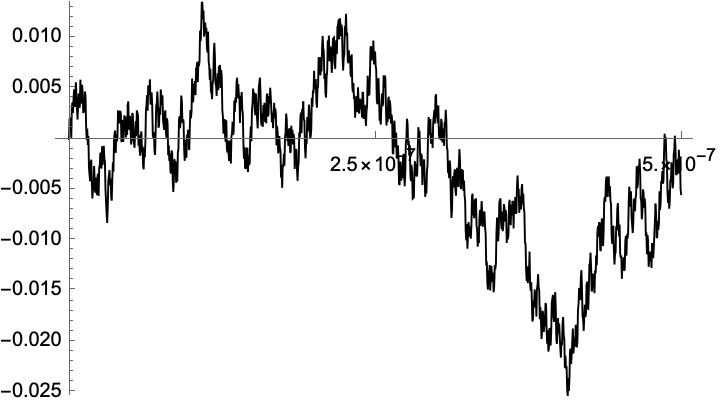
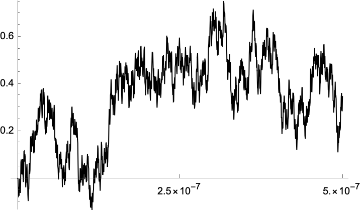
where is constant on each interval for , and is a sequence of real numbers for which the series converges absolutely. Then is well-defined and continuous due to the uniform convergence of the series in (3.7). Certain deterministic choices for yield fractal functions studied in other fields such as information theory; see [1, 2] and the references therein. When the signs of are chosen in a random manner, the expansion (3.7) becomes closely related to the Wiener–Lévy–Ciesielski expansion of Brownian motion by means of the Faber–Schauder functions, and the functions (3.7) with fixed coefficients but random signs form a non-Gaussian stochastic process with rough sample paths. More precisely, for each , let be a sequence of -valued Bernoulli random variables and define
| (3.8) |
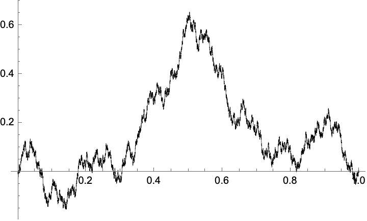
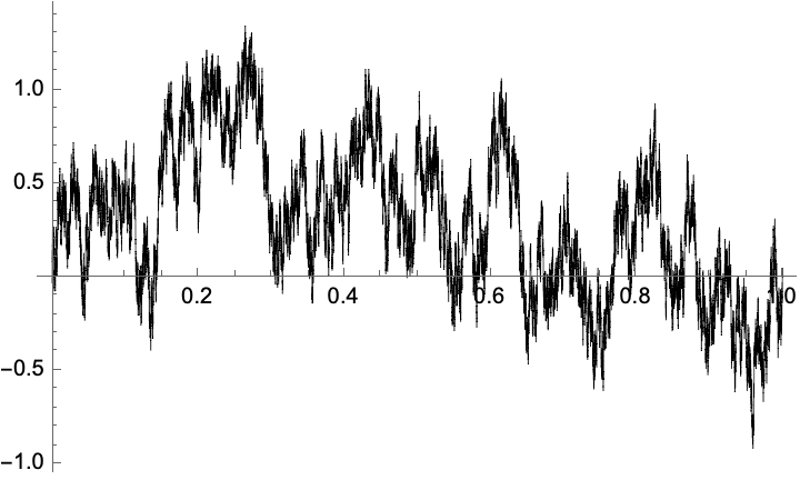
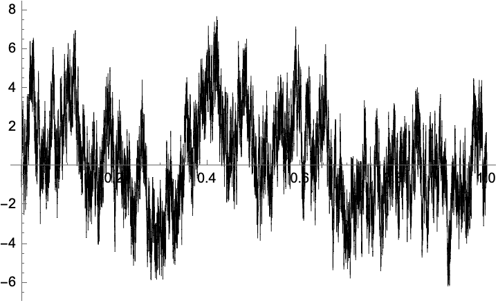
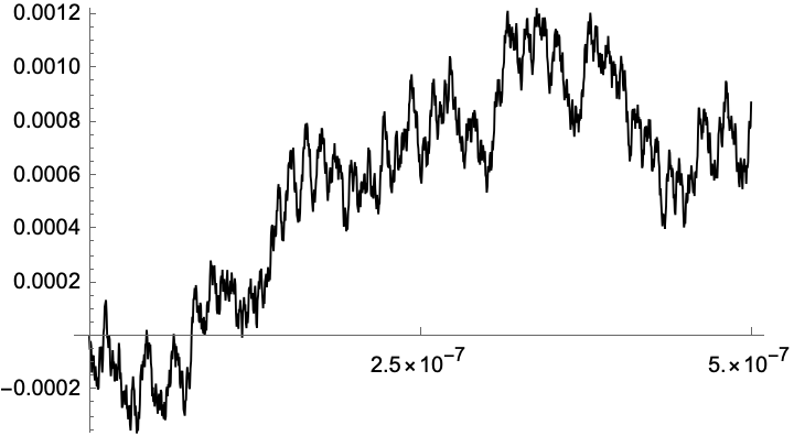
Then the following corollary states that is a stochastic process whose sample paths have the deterministic linear -variation (3.6) if the sequence satisfies the conditions on Theorem 3.3. An illustration of this stochastic process is provided in Figure 1. For the choice with , the variation of the functions (3.7) was studied in [21, 24].
Corollary 3.8.
The statements of Theorem 3.3 and of the Corollaries 3.5 and 3.6 remain fully valid for the functions of the form (3.7).
When the goal is to utilize Theorem 3.3 for the construction of functions with prescribed -variation for a given function , it can be inconvenient that the condition (3.4) is formulated in terms of the sums rather than in terms of the coefficients themselves. To deal with this issue, we are going to formulate Proposition 3.10, which will also be used in the proofs of our main results.
Remark 3.9.
Let us recall the following facts on slowly and regularly varying functions so as to put the statement of the following Proposition 3.10 into the context of Theorem 3.3.
- (a)
-
(b)
Recalling that we assume all regularly (and hence slowly) varying functions to be locally bounded, and thus locally integrable, we may define
(3.9) for a given slowly varying function . Then, according to Proposition 1.5.9 (a) in [3], the function is slowly varying and satisfies as .
Proposition 3.10.
Let be a sequence of real numbers, , and .
-
(a)
Suppose that as , let be a slowly varying function, define as in (3.9), and consider the following two conditions:
-
(i)
as .
-
(ii)
as .
Then (i)(ii).
-
(i)
-
(b)
If is a slowly varying function and , the following are equivalent:
-
(iii)
as .
-
(iv)
as .
-
(iii)
-
(c)
Any of the conditions (i)–(iv) implies as , where we take in the context of (a).
The proofs of Proposition 3.1, Theorem 3.3, Corollary 3.8, Corollary 3.5, and Proposition 3.10 are given in Section 4. Theorem 3.3 and Proposition 3.10 yield immediately the following result, which provides a simple construction for a function with prescribed -variation. When applying it to the stochastic process (3.8), it provides a straightforward way of constructing a stochastic process whose sample paths have deterministic and linear -variation; see Figure 1 for an illustration.
Corollary 3.11.
Let be a regularly varying function, , and as in (3.3).
- (a)
- (b)
Proof.
(b) Since the function is slowly varying by Remark 3.9, Proposition 3.10 (a) yields that , where . Hence, the conditions of Theorem 3.3 (b) are satisfied. Part (a) is now obvious. ∎
4 Proofs
Proof of Proposition 3.10.
(i)(ii): For any given , there exists such that for all , we have Hence, for all and ,
| (4.1) |
The Potter bounds (e.g., Theorem 1.5.6 in [3]) yield for every some such that
We hence get that for ,
Since as , we can choose small enough such that for any ,
Using this estimate in (4.1) and dividing both sides of the result by gives
| (4.2) |
Since , the inequalities in (4.2) imply that we must also have as . It follows that the left- and right-hand sides of (4.2) tend to and as , respectively. Sending now yields (ii).
(iv)(iii): It follows from the Stolz theorem and its converse given in Lemma 3.1 of [20] that the existence of one of the following limits entails the existence of the other one and that in this case both must be equal:
Moreover, if it exists, the limit on the right-hand side is equal to
and here the second factor converges to .
(c): We have
This concludes the proof. ∎
Now we turn toward proving Theorem 3.3 (and also Corollary 3.8 along the way). Following [13, 25], we let be a probability space supporting an independent sequence of symmetric -valued Bernoulli random variables. Then we define the stochastic process and set
| (4.3) |
Proposition 3.2 (a) in [25] states that is an i.i.d. sequence of symmetric -valued Bernoulli random variables. Moreover, the proof of Theorem 2.1 in [21] gives the same result in the context of Corollary 3.8, so that all subsequent observations are also valid for the functions of the form (3.7).
Note that has a uniform distribution on . Therefore, for such that all increments are less than 1,
To analyze the expectation on the right, let the truncation of be given by With the notation introduced in (4.3), we get
where in the last step we have used that due to the periodicity of . Hence, if we define
then
| (4.4) |
Thus, the -variation of is determined by the limit of the right-hand expectations as .
Proof of Proposition 3.1.
Taking , we get from (4.4) that . By Khintchine’s inequality, there exist constants and only depending on such that , and
where . From here, the assertion is straightforward.∎
Now we prove Theorem 3.3. For better accessibility, we have divided the proof into several parts.
Proof of Theorem 3.3 (a).
Assuming that , we define and
Then the exchangeability of the sequence implies that and have the same law. Clearly, in . Therefore, (4.4) yields for the choice ,
Since is continuous, this limit must coincide with the total variation of (see, e.g., Theorem 2 in §5 of Chapter VIII in [22]). Conversely, parts (b) and (c) of Theorem 3.3 will imply that can only be of finite total variation if . ∎
Proof of Theorem 3.3 (b) for .
Here, we identify the -variation at time . The linearity of the -variation will be proved subsequently. Condition (3.4) for together with our assumption implies via Proposition 1.5.1 in [3] that is regularly varying with index . Moreover, Remark 3.9, Lemma 2.2, and Proposition 3.10 yield that the law and the first moment of converge, respectively, to and to its first moment.
Let us write so that . It follows that
| (4.5) |
To deal with the first factor on the right, we estimate . First, on , we have , where is slowly varying by Proposition 1.5.7 in [3] and hence satisfies according to Proposition 1.3.6 (v) in [3]. Therefore, there exists such that
| (4.6) |
Second, to get a lower bound, we use that . Jensen’s inequality gives furthermore that
| (4.7) |
By (3.4), there is such that for all . Thus, there is such that
| (4.8) |
Combining (4.6) and (4.8) now yields
| (4.9) |
According to the uniform convergence theorem for regularly varying functions (Theorem 1.5.2 in [3]) and the fact that is regularly varying with index by Proposition 1.5.7 (i) in [3], we have
| (4.10) |
To deal with the second factor on the right-hand side of (4.5), we choose such that for all . Then, for ,
| (4.11) |
Altogether, we get
With (4.4), we thus get by sending .
To get an upper bound, we recall that is regularly varying (at infinity) with index . Theorem 1.8.2 in [3] hence yields a function that is regularly varying with index , strictly decreasing, and satisfies as well as as . Thus, the function is strictly increasing, regularly varying at zero with index , and satisfies as well as as . Let be given and choose such that for all . By (4.7), there is such that for all . For such , we get
Clearly, the factor converges to 1. Moreover, by (4.8) there is such that
As in (4.9) and (4.10), we thus get
We hence obtain the upper bound
| (4.12) |
where the right-hand side reduces to as .∎
The proof of Theorem 3.3 (b) for requires that we truncate the summation for in (4.4) at those indices for which . This is equivalent to restricting the expectation in (4.4) to the set . The following proof adapts the arguments of the proof of Theorem 3.3 (b) for to this restricted case.
Proof of Theorem 3.3 (b) for .
Let be given. The -variation of over the interval is equal to , where
This can be proved similarly as in the derivation of (4.4), see e.g. [13]. We fix and that . Recall that and let us denote for short. Then
| (4.13) |
First, we derive a lower bound for . To this end, we define for ,
Then, since ,
and so the laws of converge to in the -Wasserstein distance by Slutsky’s theorem. By combining (4.5), (4.9), (4.10), and (4.11), there is such that for all , with ,
where the last two inequalities hold due to the triangle inequality. Again, the right-most term decays to zero as . Hence, there is such that for and ,
Hence, for those and , we have and in turn
where the last step follows from (4.13) and the independence of and . Clearly, and
since by Proposition 3.10. Hence
| (4.14) |
To obtain a corresponding upper bound, we can argue exactly as in the derivation of (4.12) to get
Using again the independence of and , we find that
By (4.13), we have . Recall that as . Next, the function is slowly varying by Remark 3.9, and so
| (4.15) |
Thus, our condition (3.4) for implies that
Altogether, we conclude that . Combining this inequality with (4.14) and sending and to zero, we conclude the proof of the linearity of the -variation. ∎
The proof of part (c) of Theorem 3.3 will be prepared with the following two lemmas.
Lemma 4.1.
Under the conditions of Theorem 3.3 (c), there is a constant such that for all and all sufficiently large ,
Proof.
The function is slowly varying by Remark 3.9, and so and the sequence satisfy the conditions of Theorem 2.1. Recall from (2.8) in the proof of that theorem that there exists such that for every there is such that for all ,
and the arguments of the two square roots are positive. Now let be given and take such that for any ; this is possible by (4.15). Since is regularly varying, we have as (see, e.g., Proposition B.1.9 in [5]). Therefore, we may apply the Stolz–Cesáro theorem in its general form so as to obtain
Since , the claim follows. ∎
Lemma 4.2.
Suppose that is a sequence of nonnegative numbers converging to . Then as .
Proof.
We may assume without loss of generality that for all . Then we may write
By (3.4), the first factor on the right converges to 1. The second factor converges to by assumption. To deal with the third factor, (3.4) implies that there is such that
Theorem 1.4.1 and Proposition 1.3.6 (i) in [3] give moreover that there exists such that . Thus, if is sufficiently large such that , then
| (4.16) |
For sufficiently large , the center term can thus be expressed as , where and . The uniform convergence theorem for regularly varying functions (e.g., Theorem 1.5.2 in [3]) hence implies that
as . This concludes the proof. ∎
Proof of Theorem 3.3 (c).
We prove part (c) only for . The extension to is almost verbatim identical to the one in part (b) and hence left to the reader. We write
Then the law of is the same as that of . By Theorem 2.1, we have in . Moreover, by either Corollary 6.6 or Remark 6.7 in [6], the law of has no atoms. In particular, we have . Lemma 4.2 hence yields that -a.s. . Fatou’s lemma thus gives immediately that
To get an upper bound, we argue as in the proof of Theorem 3.3 (b) for that there exists an increasing function that is regularly varying at zero with index and satisfies for all sufficiently small as well as as . In particular, we have if is a sequence of nonnegative numbers converging to . Let be given. We choose such that for all . Since the sequence is uniformly bounded, there is such that -a.s. for all . For such , we hence have
Moreover, we see from (4.16) that there exists such that the random variables defined through
take values in for and satisfy -a.s. Hence, with denoting the index of regular variation of ,
according to the uniform convergence theorem for regularly varying functions (e.g., Theorem 1.5.2 in [3]). Hence, Lemma 4.2 and dominated convergence give that
Sending gives the desired upper bound.∎
Proof of Corollary 3.5.
(a) Taking logarithms in (3.4) and using the fact that , we get as . Hence, the result follows from Proposition 3.1.
(b) If , then (3.4) holds also if is replaced with . Hence, the assertion follows immediately from Theorem 3.3. If , then for any there is such that
Now it suffices to take such that for all and to obtain that
Sending gives the result. The case is obtained analogously. ∎
References
- [1] Pieter C. Allaart. On a flexible class of continuous functions with uniform local structure. Journal of the Mathematical Society of Japan, 61(1):237–262, 2009.
- [2] Pieter C. Allaart and Kiko Kawamura. The Takagi function: a survey. Real Analysis Exchange, 37(1):1–54, 2011.
- [3] N. H. Bingham, C. M. Goldie, and J. L. Teugels. Regular variation, volume 27 of Encyclopedia of Mathematics and its Applications. Cambridge University Press, Cambridge, 1989.
- [4] Rama Cont and Nicolas Perkowski. Pathwise integration and change of variable formulas for continuous paths with arbitrary regularity. Trans. Amer. Math. Soc. Ser. B, 6:161–186, 2019.
- [5] Laurens de Haan and Ana Ferreira. Extreme value theory. Springer Series in Operations Research and Financial Engineering. Springer, New York, 2006. An introduction.
- [6] Dorin Ervin Dutkay and Palle E. T. Jorgensen. Harmonic analysis and dynamics for affine iterated function systems. Houston J. Math., 33(3):877–905, 2007.
- [7] G. Faber. Einfaches Beispiel einer stetigen nirgends differenzierbaren Funktion. Jahresber. Dtsch. Math.-Ver., 16:538–540, 1907.
- [8] Hans. Föllmer. Calcul d’Itô sans probabilités. In Seminar on Probability, XV (Univ. Strasbourg, Strasbourg, 1979/1980), volume 850 of Lecture Notes in Math., pages 143–150. Springer, Berlin, 1981.
- [9] Hans Föllmer and Alexander Schied. Stochastic finance. An introduction in discrete time. De Gruyter Graduate. De Gruyter, Berlin, fourth revised and extended edition, 2016.
- [10] Nina Gantert. Self-similarity of Brownian motion and a large deviation principle for random fields on a binary tree. Probab. Theory Related Fields, 98(1):7–20, 1994.
- [11] Jim Gatheral, Thibault Jaisson, and Mathieu Rosenbaum. Volatility is rough. Quantitative Finance, 18(6):933–949, 2018.
- [12] E. G. Gladyshev. A new limit theorem for stochastic processes with Gaussian increments. Teor. Verojatnost. i Primenen, 6:57–66, 1961.
- [13] Xiyue Han, Alexander Schied, and Zhenyuan Zhang. A probabilistic approach to the -variation of classical fractal functions with critical roughness. Statist. Probab. Lett., 168:108920, 2021.
- [14] Masayoshi Hata and Masaya Yamaguti. The Takagi function and its generalization. Japan J. Appl. Math., 1(1):183–199, 1984.
- [15] Takayuki Kawada and Norio Kôno. On the variation of Gaussian processes. In Proceedings of the Second Japan-USSR Symposium on Probability Theory (Kyoto, 1972), pages 176–192. Lecture Notes in Math., Vol. 330, 1973.
- [16] Norio Kôno. Oscillation of sample functions in stationary Gaussian processes. Osaka Math. J., 6:1–12, 1969.
- [17] Norio Kôno. On generalized Takagi functions. Acta Math. Hungar., 49(3-4):315–324, 1987.
- [18] Michael B. Marcus and Jay Rosen. -variation of the local times of symmetric Lévy processes and stationary Gaussian processes. In Seminar on Stochastic Processes, 1992 (Seattle, WA, 1992), volume 33 of Progr. Probab., pages 209–220. Birkhäuser Boston, Boston, MA, 1993.
- [19] Michael B. Marcus and Jay Rosen. Markov processes, Gaussian processes, and local times, volume 100 of Cambridge Studies in Advanced Mathematics. Cambridge University Press, Cambridge, 2006.
- [20] Yuliya Mishura and Alexander Schied. Constructing functions with prescribed pathwise quadratic variation. J. Math. Anal. Appl., 442(1):117 – 137, 2016.
- [21] Yuliya Mishura and Alexander Schied. On (signed) Takagi–Landsberg functions: th variation, maximum, and modulus of continuity. J. Math. Anal. Appl., 473(1):258–272, 2019.
- [22] I. P. Natanson. Theory of functions of a real variable. Frederick Ungar Publishing Co., New York, 1955. Translated by Leo F. Boron with the collaboration of Edwin Hewitt.
- [23] Yuval Peres, Wilhelm Schlag, and Boris Solomyak. Sixty years of Bernoulli convolutions. In Fractal geometry and stochastics, II (Greifswald/Koserow, 1998), volume 46 of Progr. Probab., pages 39–65. Birkhäuser, Basel, 2000.
- [24] Alexander Schied. On a class of generalized Takagi functions with linear pathwise quadratic variation. J. Math. Anal. Appl., 433:974–990, 2016.
- [25] Alexander Schied and Zhenyuan Zhang. On the th variation of a class of fractal functions. Proc. Amer. Math. Soc., 148(12):5399–5412, 2020.
- [26] Teiji Takagi. A simple example of the continuous function without derivative. In Proc. Phys. Math. Soc. Japan, volume 1, pages 176–177, 1903.
- [27] S. J. Taylor. Exact asymptotic estimates of Brownian path variation. Duke Math. J., 39:219–241, 1972.
- [28] Ou Zhao, Michael Woodroofe, and Dalibor Volný. A central limit theorem for reversible processes with nonlinear growth of variance. J. Appl. Probab., 47(4):1195–1202, 2010.