Neural Network Potential Energy Surface for the low temperature Ring Polymer Molecular Dynamics of the H₂CO + OH reaction

Abstract

A new potential energy surface (PES) and dynamical study are presented of the reactive process between H₂CO + OH towards the formation of HCO + H₂O and HCOOH + H. In this work a source of spurious long range interactions in symmetry adapted neural network (NN) schemes is identified, what prevents their direct application for low temperature dynamical studies. For this reason, a partition of the PES into a diabatic matrix plus a NN many body term has been used, fitted with a novel artificial neural networks scheme that prevents spurious asymptotic interactions. Quasi-classical trajectory and ring polymer molecular dynamics (RPMD) studies have been carried on this PES to evaluate the rate constant temperature dependence for the different reactive processes, showing a good agreement with the available experimental data. Of special interest is the analysis of the previously identified trapping mechanism in the RPMD study, which can be attributed to spurious resonances associated to excitations of the normal modes of the ring polymer.

Accepted in J. of Chem. Phys. (2021)

I Introduction

The raise of the reaction rate constant at low temperatures measured in different laboratories for several organic molecules (OM) with OH and other reactants Shannon et al. (2013); Gómez-Martín et al. (2014); Caravan et al. (2015); Antiñolo et al. (2016); Ocaña et al. (2017); Heard (2018); Ocaña et al. (2019) opened a possible solution for the enigma of how organic molecules are generated in cold dense molecular clouds, below 10 K, in the interstellar medium. These reactions usually present reaction barriers, which make impossible the reaction at low temperatures in gas phase. For that reason, it was assumed that these molecules were formed on cosmic ices, in cold molecular clouds at about 10 K Hudson and Moore (1999); Watanabe et al. (2007), and then released to gas phase as they evolve to hotter structuresGarrod and Herbst (2006), such as hot cores and corinos, where they were observed Snyder et al. (1969); Ball et al. (1970); Gottlieb et al. (1973); Godfrey et al. (1973). However, recently several observations of OMs were made in UV-shielded cold cores at 10 K Remijan et al. (2006); Bacmann et al. (2012); Cernicharo et al. (2012); Vastel et al. (2014), what introduces the need of changing the model. Several hypotheses were introduced, such as the possibility of chemidesorptionCazaux et al. (2016); Oba et al. (2018), the incidence of cosmic rays Mainitz, Anders, and Urbassek (2016) and of secondary UV photons, that may induce the photodesorption. However, OMs usually present dipoles and strong binding energies, and recent experiments performed by illuminating cosmic ice precursors showed that only their photofragments are desorbed into gas phaseCruz-Diaz et al. (2016); Bertin et al. (2016). This may suggest that the origin of OMs in gas phase should be a combined mechanism, in which they are formed on ices, then their photofragments released to gas phase, where they suffer a reprocessing to finally end in the formation of the OM.

The reprocessing could be accelerated in gas phase by the huge increase of the reaction rate observed in the laboratory below 100 K Shannon et al. (2013); Gómez-Martín et al. (2014); Caravan et al. (2015); Antiñolo et al. (2016); Ocaña et al. (2017); Heard (2018); Ocaña et al. (2019). This increase is explained by the formation of a complex between the reactants, from where they tunnel to form the productsOcaña et al. (2017); Heard (2018). However, several transition state theory (TST) studies of the CH₃OH + OH reaction Siebrand et al. (2016); Gao et al. (2018); Ocaña et al. (2019); Nguyen, Ruscic, and Stanton (2019) did not get a so steep raise of the rate constant at low temperature, but it was much slower than the experimental results. They all attributed the difference to pressure effects, which at microscopic level may be attributed to the formation of complexes, between the reactants and of them with the buffer gas used in the expansions. These complexes could experience secondary collisions adding the extra energy needed to overcome the barrier. However, due to the low densities of molecular clouds the zero-pressure rate constant is needed in their models. It is therefore mandatory to check if TST methods can describe quantitatively the tunneling in the deep regime.

In this line, we have studied the dynamics of the reactions of OH with H₂CO and CH₃OH Zanchet et al. (2018); Roncero, Zanchet, and Aguado (2018); del Mazo-Sevillano et al. (2019); Naumkin et al. (2019). For this purpose, full dimensional potential energy surfaces (PESs) were fitted to accurate ab initio calculations Zanchet et al. (2018); Roncero, Zanchet, and Aguado (2018). For H₂CO + OH reaction the QCT rate constant yield a semiquantitative agreement with experimental results Ocaña et al. (2017), while for CH₃OH + OH the simulated rate constant was far too low Roncero, Zanchet, and Aguado (2018). To check if quantum effects could explain the difference, ring polymer molecular dynamics (RPMD) calculations were performed on the two PESs del Mazo-Sevillano et al. (2019), finding an excellent agreement in the case of methanol, but a similar semiquantitative agreement for the case of H₂CO. These good agreement could explain the experimental results and provide a good estimate of the zero-pressure rate constant at low temperature, but several problems still persist. First, below 100 K RPMD leads to a high trapping probability, forming complexes with extremely long lifetimes (larger than several hundreds of nanoseconds), whose trajectories cannot be finished. Therefore, the reaction rate has to be evaluated by multiplying the trapping rate constant by a ratio to products that is inferred from TST method or QCT calculations del Mazo-Sevillano et al. (2019). This could also be due to the PES, and the second problem is to improve the accuracy of the fit. This is the goal of this paper, by applying Artificial Neural Networks (ANN) techniques to fit a new PES to check if the high trapping rate persist, in one side, and to improve the comparison with experimental data.

In this work we shall explore different alternatives for multidimensional fitting with ANN techniques, including the symmetry either with permutationally invariant polynomials, PIP-NNJiang and Guo (2013); Li, Jiang, and Guo (2013); Li and Guo (2015); Jiang, Li, and Guo (2016, 2020), or with fundamental invariants, FI-NNShao et al. (2016); Lu et al. (2018). In addition, the channel towards HCOOH+H products, absent in the previous PESZanchet et al. (2018), will be included. We shall focus the attention in the problem of including long-range interactions, which are crucial to simulate the dynamics at low temperature. We shall then use the new PES to perform QCT and RPMD calculations to compare with the experimental results and to analyze the formation of long-lived complexes.

This paper is organized as follows. Firstly, a description of ab initio calculations is provided in section 2. A general description of artificial neural networks is then provided in section 3, focusing on the description of a new many-body scheme to accurately include the long-range interactions crucial in the dynamics at low temperature in section 4. With this, an overall description of the PES will be provided in section 5, showing the most important features. In section 6, we will focus on the dynamical results on this new PES, employing both QCT and RPMD methodologies, comparing with previous theoretical and experimental results. Finally some conclusions will be extracted together with several crucial questions to be addressed in the future.

II Ab initio calculations

The reactions

$$\mbox{H}_{2}\mbox{O}\mbox{H}+\mbox{O}\mbox{H}(^{2}\Pi) \rightarrow \mbox{H}\mbox{C}\mbox{O}+\mbox{H}_{2}\mbox{O}$$ (1a)

$$\rightarrow \mbox{H}\mbox{C}\mbox{O}\mbox{O}\mbox{H}+\mbox{H}$$ (1b)

are studied using the explicitly correlated coupled cluster method, RCCSD(T)-F12a/cc-pVDZKnizia, Adler, and Werner (2009), as implemented in the MOLPRO packageWerner et al. (2015). CCSD(T) calculations are considered a benchmark, and it has recently been shown that CCSD(T)-F12 is able to reach results close to CCSD(T)/CBS, even with relatively small basis sets Adler, Knizia, and Werner (2007); Ajili et al. (2013); Knizia, Adler, and Werner (2009). The effect over reactivity from an excited electronic state has been despise from the results of MRCI/cc-pVDZ calculations along the RCCSD(T)-F12 minimum energy path, since it becomes highly repulsive as the systems approach the transition states of either HCO + H₂O or HCOOH + H reaction channels. The reader is referred to the Supplementary Information for a further description.

The calculated stationary points at this level of theory are rather similar to those previously reported Zanchet et al. (2018); Francisco (1992); Alvarez-Idaboy et al. (2001); D’Anna et al. (2003); Akbar Ali and Barker (2015); Zhao et al. (2007); de Souza Machado et al. (2020). The energy of the transition state to form HCO + H₂O is very low (of $\approx$ 27 meV in this work) and is the point where larger discrepancies are found among the different works, depending on the level of theory adopted. This low energy is of the order of the expected accuracy for a system with so many electrons, and the calculated height varies from positive to negative depending of the level of theory chosen. The calculations presented here are considered to be highly accurate for the available methods at the moment, keeping the calculation of single points rather affordable for the calculation of the full dimensional PES.

Reaction 1a shows a single transition state (TS) to form HCO + H₂O, called TS1 (see figure 3), with an energy of $27.1$ meV. Before this transition state a minimum (RC1) is found at an energy of $-235.8$ meV. The minimum energy path (MEP) to form HCOOH + H, in Eq. 1b, is more complex. The system must surpass the transition state (TS2), where the OH lies over the H₂CO plane. Then, the H₂CO bends and, at the same time, the OH gets closer to the carbon atom. Finally, one of the H₂CO hydrogens leaves, forming HCOOH. The formation of $c-$HCOOH or $t-$HCOOH depends on whether the OH rotates or not from the stationary point RC4.

For the present fit, around 180000 ab initio points were added to the previously calculated for the PES of Ref. Zanchet et al. (2018). This was needed to increase the accuracy of reaction 1a, already explored in Ref. Zanchet et al. (2018), and to describe, for the first time, the channel towards HCOOH + H, in reaction 1b. The new points were calculated iteratively including points for the minimum energy paths (MEPs) and normal modes along them evaluated on intermediate fits. Also QCT and RPMD trajectories were ran on intermediate versions of the fits to populate physically accessible configurations. For each new point, the Euclidean distance Jiang and Guo (2013) to all the other points is evaluated as $d_{ab}=\sqrt{\sum_{i=1}^{15}(d_{i}^{a}-d_{i}^{b}})^{2}$, where $d_{i}^{a}$ is the $i$th interatomic distance of geometry $a$.

III Artificial Neural Networks

The use of Permutationally Invariant Polynomials (PIP) with Rydberg-type functions has been widely used to describe the PES of polyatomic systems with no many atomsAguado and Paniagua (1992); Braams and Bowman (2009). In these methods, few non-linear exponential parameters are used, while the linear coefficients of each term are fitted with a least square method. In order to obtain a PES that is invariant with respect to translation, rotation and inversion, the fit of the potential is carried out as a polynomial in terms of the internuclear distancesAguado, Suarez, and Paniagua (1994). As the number of internuclear distances increases more than the number of independent coordinate it means that, even considering low orders of the fitted polynomial, the number of coefficients necessary to carry out the fit increases enormously with a small increase of the number of atoms in the system. This implies a limitation in the application of these methods to systems of more than 6-8 atoms. Instead, in this work we make use of neural networks (NN) to fit a new PES.

Feed forward neural networksMurtagh (1991) (FFNN) are a type of functions able to transform a vectorial input into a vectorial output, in contrast to other architectures devoted to work on matrixCiresan et al. (2011) or graphDuvenaud et al. (2015) representations. This kind of neural networks has been of great interest in the field of PES fitting, where a molecular representation of the system is given to the neural network, returning its potential energy. This algorithm works in a supervised way, since the neural network is trained against a set of target energies, e.g. ab initio, usually minimizing the root mean squared error (RMSE) with the predictions.

Figure 1: Computational graph of a FFNN with two hidden layers.

A FFNN is characterized by the number of layers and the number of neurons at each layer, increasing the flexibility of the function as more layers and neurons are included. The computational graph for such a FFNN with two hidden layers is presented in figure 1. A simple rule is given to move forward in the layer structure, from the input (molecular geometry) to output (energy):

$$H_{j}^{l}=\sigma\left(\sum_{i}w_{ji}^{l}H_{i}^{l-1}+b_{j}^{l}\right),$$ (2)

where $H_{j}^{l}$ is the $j$th value of the $l$th hidden layer, $w_{ij}^{l}$ and $b_{j}^{l}$ are the trainable weights and bias in that layer and $\sigma$ is the transfer function which is, in general, not linear.

Typical choices of $\sigma$ are hyperbolic tangent or sigmoid functions between the hidden layers in the context of PES fitting , and a linear function between the last hidden layer and output layer to map the whole range of real numbers. In this work we used a logistic function, $\sigma(x)=1/(1+\exp(-x))$, between the hidden layers. The input representation for each ANN is defined as the negative exponential of each interatomic distances. The corresponding PIP of FI polynomials are evaluated on them whenever the permutational symmetry is considered. Finally, all input values are standardize to zero mean and unit standard deviation. The PIP and FI functions used are presented in the Supplementary Information.

The NN structure will be expressed in the usual way, I-H₁-$\cdots$-H_n-O, with I and O the number of neurons in the input and output layers, and $n$ hidden layers, with H_i neurons in the $i$th hidden layer. PIP-NN and FI-NN schemes, including the permutational symmetry of identical atoms, have many properties in common so artificial neural networks (ANN) will be used to refer indistinctly to either PIP-NN or FI-NN in this paper.

For each permutational symmetry group, the FI are calculated with the King’s algorithm King (2013) implemented in the computer algebra system Singular Decker et al. (2020). For many systems these FI have already been evaluated and FORTRAN routines for their evaluation are provided in https://github.com/pablomazo/FI, expanded from the original repository https://github.com/kjshao/FI.

For training ANNs we have developed NeuralPES, a Python code based on PyTorchPaszke et al. (2019) library, meant to assist at each step of the training process, beginning with data preprocessing, hyperparameter tuning and training itself.

IV Long range interaction with neural networks

The long range behaviour of a PIP PES was analyzed in Ref.Paukku et al. (2013), concluding that certain terms of the PIP expansion lead to spurious interactions in the asymptotic region due to polynomials involving distances between unconnected fragments. This was solved removing some of the polynomials that connect the fragments asymptotically in what is called “Purified Basis” Yu and Bowman (2016). An equivalent solution has been recently proposed by J. Li et al. Li et al. (2020) to be used in the fit of many body (MB) terms with PIP-NN by removing those PIPs relating unconnected distances.

In this paper we demonstrate that, on top of these terms of unconnected distances, there exist another source of spurious interactions due to the non linearity of the transfer function in the ANN. For doing so, a simplified A₂BC system is considered, focusing on the asymptote A${}_{2}\cdots$BC, such that there is no interaction between them. A PIP PES is defined as

$$V=\sum_{i}c_{i}PIP(i)$$ (3)

where $c_{i}$ are the coefficients to fit and PIP(i) is the $i$th permutational invariant polynomial. The generator of all the PIPs ($G$) for this particular permutational symmetry is:

$$G=h_{A^{1}A^{2}}^{l_{1}}h_{BC}^{l_{6}}\left[h_{A^{1}B}^{l_{2}}\cdot h_{A^{1}C}^{l_{3}}\cdot h_{A^{2}B}^{l_{4}}\cdot h_{A^{2}C}^{l_{5}}+h_{A^{2}B}^{l_{2}}\cdot h_{A^{2}C}^{l_{3}}\cdot h_{A^{1}B}^{l_{4}}\cdot h_{A^{1}C}^{l_{5}}\right]$$ (4)

where $h_{ij}=f(d_{ij})$, with $d_{ij}$ the distance between atoms $i$ and $j$, and $l_{ij}$ is and exponent. It is common to define $h_{ij}=\exp(-\alpha d_{ij})$, such that $h_{ij}$ tends to zero as the distance tends to infinity. In this situation only the PIPs where $l_{2}=l_{3}=l_{4}=l_{5}=0$ survive in the long range:

$$G^{(\infty)}=h_{A^{1}A^{2}}^{l_{1}}h_{BC}^{l_{6}}$$ (5)

Setting $\max(l_{i})=1$ the following set of PIPs is defined:

$$PIP=\{h_{A^{1}A^{2}},\,h_{BC},\,h_{A^{1}A^{2}}\cdot h_{BC}\}$$ (6)

Therefore, the PES in the asymptote is evaluated as

$$V^{(\infty)}=c_{1}\cdot h_{A^{1}A^{2}}+c_{2}\cdot h_{BC}+c_{3}\cdot h_{A^{1}A^{2}}\cdot h_{BC}$$ (7)

Notice that, through the third term in the expansion a force between A₂ and BC fragments arises, even though they were set at an infinite distance. This PIP set could be purified by just removing the third function, hence disconnecting both fragments. At this point, the asymptotic potential energy surface would depend linearly on both fragment distances, so no spurious interactions are introduced up to now.

The next step is to show that even when the purified PIP set is used, PIP-NN introduces spurious interactions. In a PIP-NN with only one hidden layer, the energy is evaluated as

$$V = \sum_{j}w_{Ej}H_{j}+b_{E}$$ (8)

$$H_{j} = \sigma\left(\sum_{i}w_{ji}PIP(i)+b_{j}\right),$$ (9)

where $w$ and $b$ are the weight matrices and bias vectors, $\bm{H}$ is the hidden layer and $\sigma$ is the transfer function, which in general is not linear. The values of the neurons of the hidden layer evaluated on the purified PIP set become

$$H_{j}=\sigma\left(w_{j1}\cdot h_{A^{1}A^{2}}+w_{j2}\cdot h_{BC}+b_{j}\right).$$ (10)

Since $\sigma$ is not linear, a connection between both fragments is introduced and, with that, an spurious force between them arises. $\partial V/\partial h_{A^{1}A^{2}}$, which ultimately relates with the force $A^{1}$ and $A^{2}$ experience is

$$\frac{\partial V}{\partial h_{A^{1}A^{2}}}=\sum_{j}w_{Ej}w_{j1}\sigma^{\prime}\left(w_{j1}\cdot h_{A^{1}A^{2}}+w_{j2}\cdot h_{BC}+b_{j}\right),$$ (11)

being clear that there is always a dependence with the BC fragment.

This same derivation can be develop with a set of FI, arriving to the same conclusion. Moreover, this problem is magnified when more than one hidden layer is introduced. This spurious interactions lead to an energy transfer between the fragments, that will have a critical effect in dynamical studies, specially at low collision energies, where trajectories could even be reflected. We may then conclude at this point, that the main source of spurious interactions in a PIP-NN or FI-NN is the non linearity of the transfer function.

Although it would yield to a very low fitting error, the above arguments show that it is not possible to fit the PES with one ANN since a residual interaction persists between the reactants at long distances. This causes small changes in the internal energies of each fragment, introducing errors that strongly affect the dynamics at low energies, making inconvenient the use of PIP or FI-NN PES that expand the whole configuration space.

One possible solution is to separate the PES in two regions, short and long range, connected by a switching function Li and Guo (2014). The long range term would be a well behaved separable function and the short range an ANN PES. The main difficulty with this functional form is to tune the switching function to produce a smooth change between both regions, specially as the dimensionality of the system increases. This can also have a huge effect when studying low energy or temperature dynamics of the system, due to the possible presence of spurious matching problems.

In this work we propose to use a partition of the potential energy as the one used in the previous PESsZanchet et al. (2018); Roncero, Zanchet, and Aguado (2018); Aguado et al. (2010); Sanz-Sanz et al. (2013), were a diabatic matrix, $V^{diab}$, is used to produce a first order PES corrected with a six-body term, as expressed by

$$V=E_{0}^{diab}+V^{6C},$$ (12)

where $E_{0}^{diab}$ is the lowest eigenvalue of $V^{diab}$. This matrix is of dimension $N\times N$, being $N$ the number of rearrangement channels, each of them describing reactans or products fragments, and the interaction between them, including long range interactions. This matrix is analogous to those previously used Zanchet et al. (2018); Roncero, Zanchet, and Aguado (2018), and is described in detail in the SI. In the present implementation of $V^{diab}$, the accuracy of each fragment of the PES has been increased by replacing them by ANN fittings.

The main advantage of this form is that the diabatic matrix captures the basic features, namely the long range interactions in each rearrangement channel and a first approximation to short range interactions, only using PESs for each of the fragments and their interactions on each rearrangement channel. This idea is based on triatomics-in-molecules (TRIM) Aguado et al. (2010); Sanz-Sanz et al. (2013) and diatomic-in-molecules (DIM)Ellison (1963); Ellison, Huff, and Patel (1963), that allows an accurate description of the fragments of physical relevance as well as the interactions among them, both short and long range.

V Potential Energy Surface: NN Six-body term

For the six-body term, $V^{6C}$, we propose to use the partition

$$V^{6C}=S\cdot V^{ANN},$$ (13)

where $S$ is the switching function, designed to be zero as the system tends to any of the asymptotic regions, removing the spurious interaction from the $V^{ANN}$, the PIP-NN or FI-NN function, trained to the difference between the ab initio energies and $E_{0}^{diab}$, $i.e.$ it should tend to zero at long distances. In this way, the switching function ensures once more that the MB term will go to zero in the desired regions, and the fragments in the asymptotic region will not be affected by spurious interactions. On top of that, notice that it is not necessary to purify the set of invariants anymore, since is the $S$ function which removes the spurious connections.

In order to stress the importance of removing the long range spurious interaction in ANN PES, the energy of the H₂CO and OH fragments has been followed along two QCT trajectories, being both fragments well separated so that there is no physical interaction between them. In the first trajectory, $V^{6C}=V^{ANN}$ and in the second one $V^{6C}=S\cdot V^{ANN}$. The results are shown in figure 2. It is clear that when the $S$ function is not included to build the six-body term, both fragments experience an spurious interaction that makes their energy change along the trajectory. This transfer is of about 10 meV, comparable to the relative kinetic energy at low collisional energy. This interaction is completely removed by the switching function as it becomes evident by the constant energy of the fragments in dashed lines.

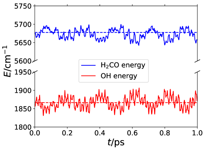
Figure 2: Energy of H₂CO and OH fragments in two QCT trajectories with the fragments set at a large distance so there is no physical interaction between them. With dashed lines a trajectory in which $V^{6C}=S\cdot V^{ANN}$ and with solid lines one where $V^{6C}=V^{ANN}$.

The asymptotic channels to consider in this system are H₂CO + OH, HCO + H₂O and HCOOH + H. The switching function ($S$) is a product of hyperbolic tangents depending on the distances $d_{CO}$, $d_{CH_{1}}$ and $d_{CH_{2}}$, so permutational symmetry of H₂CO is preserved.

$V^{ANN}$ is fitted with NeuralPES program through a FI-NN with a structure 21-80-80-1, meaning that 21 fundamental invariants are required for taking into account the permutational symmetry of the two formaldehyde hydrogen atoms. The FIs are evaluated over the negative exponential of the interatomic distances. The reader is referred to the Supplementary Information for the hyperparameter description used here.

Table 1: RMSE evaluated over each energy range for the diabatic term and the full PES.

$\bm{E}/eV<$	Points	$\bm{E_{0}^{diab}}$ / meV	$\bm{V}$ / meV
$0.0$	87356	$369.38$	$39.18$
$1.0$	218522	$411.41$	$51.98$
$2.0$	245978	$469.64$	$65.79$
$3.0$	261437	$523.92$	$86.45$
$4.0$	269743	$564.00$	$92.05$
$5.0$	274326	$584.60$	$105.60$

The RMSE of $E_{0}^{diab}$ and the fitted PES are presented in table 1. The ANN $V^{6C}$ term reduces the fitting error by almost a factor of 10 for the lower energy ranges.

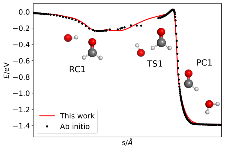
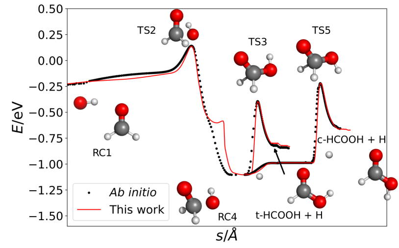
Figure 3: Minimum energy paths for the formation of HCO + H₂O (left) and HCOOH + H (right), both cis and trans rotamers. The geometries of the stationary points are represented along the path.

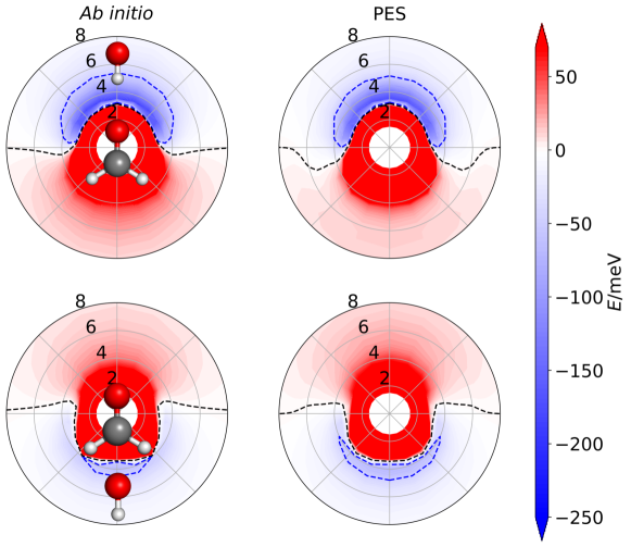
Figure 4: Energy of the system when OH approaches H₂CO in the plane. On the top (below) panels, the H (O) of OH always faces the H₂CO molecule. Black and blue isolines represent energies of 0 meV and -50 meV, respectively. Distance is expressed in Å. The H₂CO and OH fragments are only meant to serve as a reference, they are not at scale.

In figure 3 the ab initio and the PES minimum energy paths for reactions to HCO + H₂O and HCOOH + H are shown. In both cases we find a very good agreement between the paths, with the only exception of a shoulder that appears in the HCOOH + H products channel. This is not expected to have any effect on the dynamics since it is well below the reactants asymptote. We find an improvement with respect to the previous PES in the description of the region of stationary point RC1, which was geometrically not well located. Also, another local minima on the reactants rearrangement channel, not related to the minimum energy path, have been improved, what is of importance for a reaction with such a roaming behaviour.

The short range region of the PES is compared against ab initio results in figure 4. In general, the PES is very well behaved, showing a perfect agreement for both attractive and repulsive regions.

A very good agreement is also found in the normal mode frequencies on the different transition states as can be checked in the table presented in the Supplementary Information. High frequency modes have been considerably improved, in part due to a better description of the fragments PESs. It is also found that, in general, low frequency modes present greater differences, since they relate with flatter regions of the PES that can be more challenging to fit.

VI Dynamical Results

VI.1 QCT results

QCT calculations were carried with an extension of miQCT codeDorta-Urra et al. (2015); Zanchet, Roncero, and Bulut (2016) for $N$ atom systems. The reaction cross section $\sigma(E)$ is calculated at fixed collision energy with the reactants in their ground vibrational and rotational states as:

$$\sigma(E)=\pi b_{max}^{2}P_{r}(E)$$ (14)

where $b_{max}(E)$ is the maximum impact parameter and $P_{r}(E)$ the reaction probability at a given collision energy. The initial conditions of the internal degrees of freedom of the fragments have been calculated with the adiabatic switching method Ehrenfest (1917); Nagy and Lendvay (2017). The remaining initial conditions are set by random numbers according to the usual Monte Carlo method Karplus, Porter, and Sharma (1965). The initial maximum impact parameter is set according to the capture model for a dipole-dipole interaction Levine and Bernstein (1987); Zanchet et al. (2018) shown in Fig. 5 along with the converged $b_{max}$.

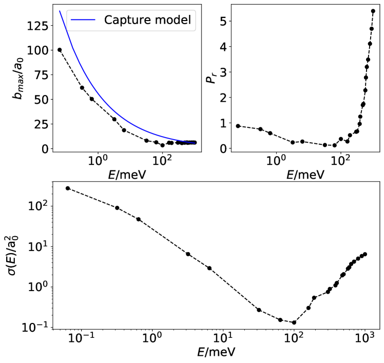
Figure 5: QCT results at fixed collisional energy for the formation of HCO + H₂O. On the top left panel, the maximum impact parameter, on the top right panel the reaction probability and in the lower panel, the reactive cross section.

The reactive cross section for the formation of HCO + H₂O is presented in figure 5, calculated from more than $5\times 10^{4}$ trajectories at each collisional energy within $b_{max}(E)$. The present QCT results have the same qualitative behaviour as those obtained with a previous PESOcaña et al. (2017); Zanchet et al. (2018), and reactive cross section experiences a huge increase as the collisional energy decreases below 100 meV, even at energies lower than the transition state energy barrier, at 27 meV. This increase in the reactive cross section is explained by an enormous increase of the maximum impact parameter, while the reaction probability remains constant or slightly increases.

The reaction at high relative collisional energy is characterized by a direct mechanism in which OH and H₂CO collide and either react or fly apart. At low collisional energies the reaction is dominated by the long range, dipole-dipole, interaction which rotates and orients the reactants as to maximize their interaction, capturing the trajectory for high values of the impact parameter. This leads to a rotational excitation of the system as the reactants become closer that traps the system for long times, since it is improbable to stop the rotation turning it into translation. Direct and trapped QCT trajectories are similar to the RPMD ones, shown in figure 9, with the difference that trapped trajectories live much less, as will be discussed below.

The reaction probability does not got to zero for collisional energies below the potential barrier, since the zero-point energy (ZPE) is enough to overcome it. Still, there must exist couplings between the orthogonal degrees of freedom that promote the energy transfer among them. This coupling becomes favoured by the roaming-like mechanism and the huge complex lifetimes experienced at low collisional energies.

The QCT reaction rate constants have been calculated at constant temperature, with the reactants in their ground vibrational states and considering their rotational distribution. Only the two states that correlate with the ground spin-orbit state, OH(${}^{2}\Pi_{3/2}$), react, so the electronic partition function is

$$q_{e}(T)=\frac{1}{1+\exp(-200.3/T)},$$ (15)

and the reaction rate constant is evaluated as

$$k(T)=q_{e}(T)\sqrt{\frac{8k_{B}T}{\pi\mu}}\pi b_{max}^{2}(T)P_{r}(T),$$ (16)

where $b_{max}(T)$ and $P_{r}(T)$ are the maximum impact parameter and reaction probability at constant temperature, and $\mu$ is the reduced mass of the OH, H₂CO system.

The calculated reaction rate constants are shown in figure 6 along with the experimental results in the temperature range from 22 K to 1200 K, together with rates calculated earlier with another PES Ocaña et al. (2017); Zanchet et al. (2018).

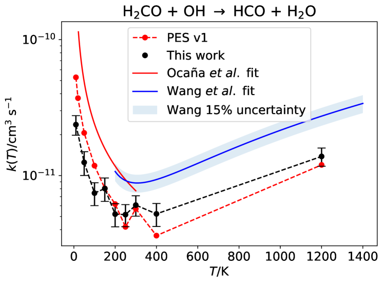
Figure 6: QCT reaction rate constant at constant temperature for HCO + H₂O formation. With black points, the results obtained in this work. The error bars are two times the standard error of the Monte Carlo integration Karplus, Porter, and Sharma (1965). With red points, the results from our previous PES Zanchet et al. (2018), With solid lines, the recommended fit from Ocaña et al. Ocaña et al. (2017) in red and from Wang et al. Wang, Davidson, and Hanson (2015) in blue.

The reaction rate constant behaviour with temperature is basically the same for the two PESs above 100 K, but below this temperature there is a quantitative difference between both of them, although both reproduce the increase experimentally shown. It is not surprising that the reaction rate constants calculated with the two PESs is not well reproduced at high temperatures, since only the vibrational ground state of the fragments is being considered. Still, there is a factor of about 1.5 between our results and the experimental ones from Wang et al. at 300 K. This difference increases as the temperature lowers, with respect to experimental results and also between both PES. The discrepancies between the two PESs could be attributed to variations in the transition state region. Due to the relatively small height of the TS and the high anharmonicity of this region, tiny differences, below the fitting error, can lead to differences in dynamical behaviour.

The reaction to form HCOOH + H is secondary with respect to the formation of HCO + H₂O. In particular, R. A. Yetter et al. Yetter et al. (1989) measured the kinetic rate constants for the formation of HCO + H₂O to be $(7.75\pm 1.24)\times 10^{-12}$ cm³ molecule^-1 s^-1, in good agreement with the present results, and $0.2^{+0.8}_{-0.2}\times 10^{-12}$ cm³ molecule^-1 s^-1 for HCOOH + H at 300 K.

No formation of HCOOH + H was observed in the RPMD trajectories described below, because of the low reaction probability of this channel and the impossibility to enrich the RPMD statistics. At fixed collisional energy, the only reactivity was obtained in QCT calculations above 300 meV, which is consistent with a barrier height of 276.0 meV, including ZPE. This reaction follows a direct mechanism, where the OH approaches the H₂CO in a conformation close to the one in TS2. Indeed, the maximum impact parameter for this process is about 3 times smaller than the one for HCO + H₂O at collisional energies of 300 meV, decreasing the gap at 1 eV to 1.5. As the collisional energy increases so does the reaction probability, since the system has more energy in the reaction coordinate. These results are summarized in figure 7.

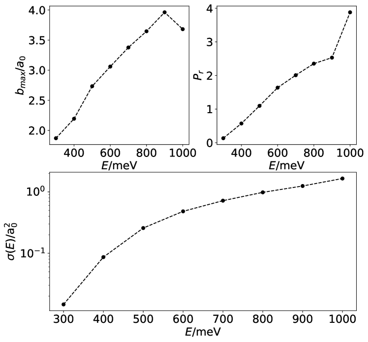
Figure 7: QCT results at fixed collisional energy for the formation of HCOOH + H. On the top left panel, the maximum impact parameter, on the top right panel the reaction probability and in the lower panel, the reactive cross section.

At fixed temperature, reactivity was obtained above 900 K. It is important to remember that only reactivity from reactants in their ground vibrational states is being taken into account. Our results are in good agreement with the ones calculated by G. de Souza et al. de Souza Machado et al. (2020) with the canonical variational transition state method (CVTST) and are shown in Fig. 8.

Figure 8: QCT reaction rate constant at constant temperature for HCOOH + H formation. The error bars are two times the standard error of the Monte Carlo integration Karplus, Porter, and Sharma (1965). In red line the results obtained by G. de Souza et al.de Souza Machado et al. (2020).

VI.2 RPMD results

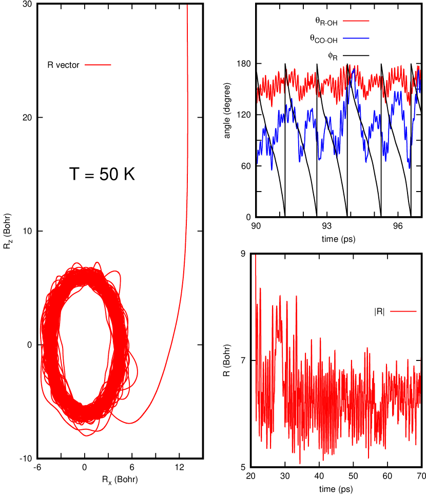
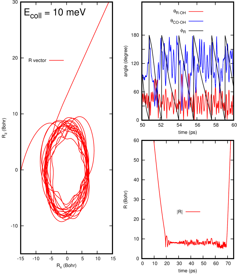
Figure 9: Typical trapped RPMD trajectory (left 3 panels) obtained at 50 K. Right panels show a typical QCT trajectory for high (red) initial impact parameter, at fixed collisional energy of 0.1 meV. In each case, the left panel shows the components $R_{x}$ and $R_{z}$ of the vector, R, connecting the centers of mass of the reactants along the trajectory. The right bottom panels show the modulus of R as a function of time. The right top panels show the evolution of the angles: between ${\bf R}$ and OH internuclear vector, $\theta_{R-OH}$, between the CO and OH internuclear vectors, $\theta_{CO-OH}$ and the azimuthal angle associated to R, $\phi$.

Quantum effects, such as tunneling and zero-point energy, are important at the low temperatures of interest here. Exact quantum calculations are not feasible in this system, and one of the most successful alternative methods is Ring Polymer Molecular Dynamics (RPMD) Craig and Manolopoulos (2004, 2005a, 2005b); Suleimanov, Collepardo-Guevara, and Manolopoulos (2011); Suleimanov, Aoiz, and Guo (2016), which is used in this work. RPMD is a semiclassical formalism based on Path Integral Molecular Dynamics (PIMD), that includes quantum effects such as ZPEPérez de Tudela et al. (2012) and tunnelingPérez de Tudela et al. (2014). RPMD has been successfully applied to many reactions, with barriers or deep wells Suleimanov, Aoiz, and Guo (2016); Suleimanov et al. (2018). Here we use the dRPMD programSuleimanov et al. (2018), a direct version of the RPMD method born as an alternative to the RPMDrate code Suleimanov, Allen, and Green (2013) to deal with reactions with no barriers. dRPMD is parallelized to allow long propagations at low temperatures, requiring many replicas or beads, N_b. The direct RPMD consists in two steps, thermalization and real-time dynamics.

The thermalization is a constrained PIMD simulation, using the Andersen thermostat Andersen (1980) and freezing the distance between the two reactants at 120 $a_{0}$. This propagation is performed during 10⁴-10⁵ steps, depending on the temperature, to warrant convergence of the initial ZPE of each fragment. At the end of the thermalization the relative position and velocities of the two reactants are reoriented, imposing a maximum initial impact parameter, similar to QCT calculations.

In the second step, the constrain and the thermostat are removed, leading to the classical evolution of a system consisting on $N_{atoms}\times N_{b}$ particles, which are propagated using a second order simplectic operator. In previous RPMD calculations del Mazo-Sevillano et al. (2019), the simplectic propagation is separated in two steps: first the free polymer and second the real potential terms. The free polymer propagation was done using a Fourier transform (FT) Suleimanov, Allen, and Green (2013), and, being nearly exact, allows a large time step. In the previous RPMD calculations del Mazo-Sevillano et al. (2019); Naumkin et al. (2019) it was also found that, for temperatures below 100 K, many trajectories were trapped in the complex well in the reactants channel. Those trapped trajectories lived for more than 500 ns, and were too long to be finished. So long-lived complexes, as compared to those obtained in QCT calculations (of several ps), could be explained by the reduction of the available reactants phase space produced in RPMD, in which ZPE is taken into account. However, it is also known that RPMD may show spurious resonances Witt et al. (2009); Rossi, Ceriotti, and Manolopoulos (2014); Jang, Sinitskiy, and Voth (2014); Korol, Bou-Rabee, and III (2019), which can be attributed to polymer normal mode excitations probably accessed when the frequencies of these modes are close to the frequencies associated to the “physical” system. These spurious resonances seem to be enhanced when the free ring polymer is propagated as a separate entity and several alternatives have been proposed Jang, Sinitskiy, and Voth (2014); Korol, Bou-Rabee, and III (2019).

The choice made in this work is not to propagate the free ring polymer. Instead, we separate the ring polymer Hamiltonian in physical kinetic energy and total potential, containing the PES among the $N_{atoms}$ atoms and the harmonic oscillators among the beads of the same atoms. This implies to reduce the time step to approximately $\Delta t/\sqrt{N_{b}}$, with $\Delta t$ the time step used in the FT propagation. This reduction of the time step increases the computational time, but when using parallel computers the present factorization reduces the communication to only neighbor processors, thus allowing a higher speed up of the parallelization.

The parameters used for the calculation of the RPMD rate constants for different temperatures are listed in table 2. At the end of each RPMD trajectory, the product channel is determined by analyzing the centroid, similarly to what is done in QCT calculations. What is different in RPMD calculations, is that there is an increasing probability of trapped trajectories as temperature decreases below 300 K. Those trapped trajectories are formed following an orbit similar to the QCT orbit of Fig. 9 as those shown in previous RPMD calculations in this systemdel Mazo-Sevillano et al. (2019); Naumkin et al. (2019): the long range interaction deviates the initial trajectories for rather long impact parameters, increasing the end-over-end angular momentum and the rotation of each of the two reactants. These trajectories get then trapped orbiting continuously keeping the relative orientation of the two reactants fixed, close to the geometry of reactant well, RC1. What is different from QCT calculations, is that these trapped orbits live very long times, longer than $t_{max}$ = 10 ns in this case, when they are stopped. Thus we give separate probabilities for direct (reactive RPMD trajectories) and trapped trajectories in table 2. The rates for direct reaction and trapping processes are then evaluated through equation (16), as listed in table 2

Table 2: Parameters of the direct RPMD and rate constants.

$T$/K	$N_{b}$	$N_{total}$	$t_{max}$/ns	$b_{max}^{dir}/a_{0}$	$b_{max}^{trap}/a_{0}$	$P_{dir}$	$P_{trap}$	$k_{dir}$ / cm3 s-1	$k_{trap}$/ cm3 s-1
1200	144	10000	$1.0$	$8.44$	$0.00$	$0.025$	$0.00$	$1.31\times 10^{-11}$	0$.00$
1000	48	2454	$0.1$	$5.82$	$0.00$	$0.048$	$0.00$	$1.10\times 10^{-11}$	0$.00$
800	144	3749	$0.1$	$7.93$	$0.00$	$0.019$	$0.00$	$7.21\times 10^{-12}$	0$.00$
600	144	4649	$0.1$	$6.76$	$0.00$	$0.026$	$0.00$	$6.67\times 10^{-12}$	0$.00$
400	96	6695	$0.1$	$6.93$	$0.00$	$0.016$	$0.00$	$3.82\times 10^{-12}$	0$.00$
300	240	30000	$1.0$	$11.93$	$7.86$	$0.003$	$2.59\times 10^{-4}$	$2.18\times 10^{-12}$	7$.11\times 10^{-14}$
200	384	20000	$1.0$	$11.78$	$13.82$	$0.005$	$2.01\times 10^{-3}$	$2.58\times 10^{-12}$	1$.54\times 10^{-12}$
100	768	1000	$1.0$	$12.95$	$16.60$	$0.003$	$1.94\times 10^{-1}$	$1.92\times 10^{-12}$	1$.83\times 10^{-10}$
50	1536	400	$1.0$	$13.39$	$18.96$	$0.015$	$5.89\times 10^{-1}$	$7.15\times 10^{-12}$	5$.72\times 10^{-10}$
20	3072	143	$1.0$	$14.53$	$21.43$	$0.048$	$6.40\times 10^{-1}$	$1.75\times 10^{-11}$	5$.11\times 10^{-10}$

The trapping mechanism becomes significant at temperatures below 200 K, where trajectories finished after 10 ns without dissociation or reaction. This results perfectly mimic the ones from our previous work del Mazo-Sevillano et al. (2019) as shown in figure 11. As compared to our previous PES, the trapping mechanism begins at temperatures slightly higher, around 300 K. With respect to the direct mechanism rate, the difference found in the QCT study seems to magnify, what on top of what has already been said in the previous section, it is worth noting that some of the errors may emerge from a poorer statistic, due to the huge computational cost of RPMD trajectories at these low temperatures. A typical trapped RPMD trajectory is shown in the right panels of Fig. 9, compared with a direct and complex-forming QCT trajectories shown in the right panels of Fig. 9. The first difference in both trajectories is that RPMD trajectory keeps trapped for much longer times than QCT trajectory, that actually manages to break the reactive complex in the propagation time. Once the two reactants collide, $\phi_{R}$ oscillates quasi periodically in both cases, but the angle $\theta_{R-OH}$ vector keeps almost constant. This behaviour is endorsed by the $\theta_{CO-OH}$ angle, and the only appreciable difference is that QCT amplitudes have larger variations.

With respect to our previous work del Mazo-Sevillano et al. (2019), not only the partition of the RP Hamiltonian has been varied, but also the time step, $\Delta t$, has been reduced by a factor of 10 and the number of beads used in the low temperature calculations has been considerably increased, in order to check whether or not long-lived complex lifetimes are artificially due to poor convergence. The computational cost of this PES has been considerably reduced, what has enabled to perform this kind of study. However, the formation of extremely long trapped trajectories persist here, as can be seen in figure 11. Therefore, we discard the possibility of this results being a lack of convergence of the calculations. Similar behaviour was also found for other reactions at low temperature, OH + CH₃OHdel Mazo-Sevillano et al. (2019), D + H${}_{3}^{+}$Bulut et al. (2019) and H₂ + H${}^{+}_{3}$Suleimanov et al. (2018). We therefore conclude that the trapping is a rather general outcome of RPMD calculations at low temperature.

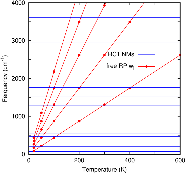
Figure 10: RC1 complex normal mode frequencies (blue) and first five $\omega_{i}$ free ring-polymer frequencies versus temperature.

An increase of complex lifetimes when including quantum effects is expected and can be explained according to the statistical theory RRKMMarcus (1952a, b) by the descent of accesible dissociative states in the RPMD calculations with respect to the QCT ones, because ZPE is included. However, the impossibility to end the trapped trajectories, dominant at low temperatures, seems to indicate that RPMD method fails to reproduce the real lifetime of the reaction complexes. This is attributed to the appearance of spurious resonances as those reported previously Witt et al. (2009); Rossi, Ceriotti, and Manolopoulos (2014), that appear when the frequency of the complexes are of the order of those of the ring polymer modes. The normal modes of the free ring polymers Richardson and Althorpe (2009) are given by $\omega_{k}=2N_{b}k_{B}T/\hbar\sin(|k|\pi/N_{b})$, with $k_{B}$ being the Boltzmann constant and $-N_{b}/2\leq k\leq N_{b}/2$. The lowest frequency mode, $k=1$, for large $N_{b}$ can be approximated by $\omega_{1}\approx 2\pi Tk_{B}/\hbar$, and when this quantity is of the order of the lower frequency of the reaction complex, the energy flow between the “physical” and “free ring-polymer” modes may be enhanced, giving rise to spurious resonances, in which the energy is stored in the free ring-polymer normal modes. The lower $\omega_{i}$ are plotted as a function of temperature and compared with the physical frequencies of the H₂CO-complex in Fig. 10. Clearly at $\approx$ 100 K, the first RP normal mode is of the order of the lower RC1 normal modes. As temperature decreases, there are Ring-polymer modes in near resonance with several physical modes of the RC1 complex, favoring the energy transfer. Since the density of the RP modes is large, the energy is stored there for very long times, giving rise to artificial trapping or spurious resonances.

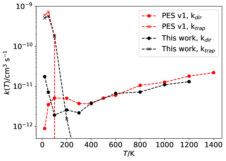
Figure 11: Reaction and trapping rates for the present PES, compared with the ones from out previous fit.

Several solutions have been proposed to solve the problem of spurious resonances in RPMD calculations of spectra Witt et al. (2009); Rossi, Ceriotti, and Manolopoulos (2014). Among them, the inclusion of a thermostat to the internal modes of the ring polymer during the dynamics Rossi, Ceriotti, and Manolopoulos (2014) is considered here that may affect the reaction dynamics, because the extra energy of the beads is expected to flow to the physical bonds, producing their fragmentation. A detailed analysis needs to be done before applying it to reactive collisions at low temperatures. Instead, in order to get the total reaction rate constant we have to look for an alternative method to consider the fragmentation ratio of the trapped trajectories: back to reactants (redissociation) and tunneling through reaction barriers to products (tunnel). Under this assumption, the total reaction rate becomes:

$$k(T) = k_{dir}(T)+k_{CF}(T)$$ (17)

$$k_{CF}(T) = k_{trap}(T)\frac{k_{tunnel}(T)}{k_{tunnel}(T)+k_{rediss}(T)},$$ (18)

where $k_{dir}$ is the rate constant for the direct mechanism and $k_{CF}$ is the product of the trapping rate constant and the ratio of tunneling trajectories towards products. This approach was suggested beforedel Mazo-Sevillano et al. (2019); Naumkin et al. (2019), and the ratios were obtained either from TST or QCT methods. Here we adopted the QCT reaction probability as

$$\frac{k_{tunnel}(T)}{k_{tunnel}(T)+k_{rediss}(T)}\approx P_{r}^{QCT}(T),$$ (19)

that is, $\approx 1\%$ for collision energies below 1 meV. This classical estimate is justified by the small height of the TS, that can even be reduced due to anharmonic effects. The resulting RPMD reaction rate constants are shown in figure 12 compared with previous results. The behaviour of both results are similar and always below the experimental values.

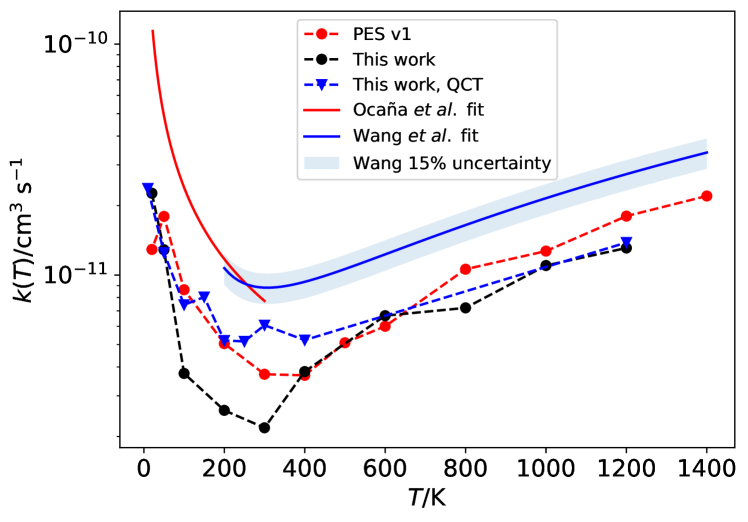
Figure 12: RPMD reactive rate constant for HCO + H₂O formation. Black points represent the RPMD results obtained in this work. Blue triangles represent the QCT results obtained in this work. Red points are the results from our previous PES Zanchet et al. (2018). Solid lines show the recommended fit from Ocaña et al. Ocaña et al. (2017) in red and from Wang et al. Wang, Davidson, and Hanson (2015) in blue.

Black points and blue triangles represent the RPMD and QCT results obtained in this work, respectively. Red points are the RPMD results from our previous PES Zanchet et al. (2018). Solid lines show the recommended fit from Ocaña et al. Ocaña et al. (2017) in red and from Wang et al. Wang, Davidson, and Hanson (2015) in blue.

The difference between simulated and experimental rate constants for T$>$400 K is attributed to the appearance of other mechanisms, such as non-adiabatic contributions of excited electronic state, and/or a lack of accuracy to describe other channels such as H + HCOOH product channel. In this work we focus on the lower temperature behaviour. Here the problem is to determine the tunneling/redissociation fraction of the trapped RPMD trajectories. Such study is fundamental for astrochemistry, since it is necessary to use the pure zero-pressure rate constant for the formation of OM in cold environments.

Also, it is important to determine the life-time of the reaction complexes to establish the role of complexes (or pressure) in the measured rate constants in CRESU experiments. Work in this direction is now on the way, following the preliminary arguments already publishedNaumkin et al. (2019).

VII Conclusions

In this work a new full dimensional potential energy surface has been developed for the title reaction based on artificial neural networks. The long-range behaviour of the ANN has been analyzed in detail. A source of spurious interactions has been identified due to the non linearity of the transfer function in the ANN, that mixes the internal degrees of freedom of each of the polyatomic fragments. These spurious interactions change the energy of the fragments at very long distances introducing artifacts in the dynamics at low energies, thus becoming inappropriate to study reactivity at low temperatures.

To solve this problem, a new factorization of the potential is proposed consisting in two terms, a diabatic matrix and a full dimensional term, $V^{MB}$, expanded using neural networks. In the diabatic matrix, the diagonal elements describe each rearrangement channel, including the potential of each independent fragment plus their interaction among them, with the long range interaction properly set. Thus, $V^{MB}$ fits the difference and tends to zero at intermediate distance. This term is further multiplied by a switching function to fully remove the spurious long range interaction introduced by the artificial neural network function. The present potential is more accurate than the previous oneZanchet et al. (2018) and also incorporates the channel towards HCOOH + H product channel.

This PES has been used to calculate the reaction rate constants using QCT and RPMD methods. It is found that the HCOOH + H products present a near negligible contribution at the energy range considered. The HCO + H₂O reaction rate constant presents a non-Arrhenius V-shape as a function of temperature, dominated by a direct mechanism at high temperatures and a complex-forming at low energies, as it was also found in the previous PESdel Mazo-Sevillano et al. (2019) and in qualitative agreement with the available experimental data Ocaña et al. (2017).

In spite of the changes done in the calculations, the RPMD results show an increasing trapping probability as temperature decreases, as reported beforedel Mazo-Sevillano et al. (2019). This is attributed to the presence of spurious resonances occurring when the free ring-polymer normal mode frequencies enter in near resonance with the low intermolecular normal modes frequencies. It is crucial to determine the life-time of these complexes and the fragmentation ratio in order to properly determine the zero-pressure reaction rate constant, needed in astrophysical models, and to determine the role of complexes in the measurements made in laval expansions. Some work in these directions are now-a-days under way.

VIII Supplementary Material

See supplementary material for the multi-reference calculations of ground and first electronic states along the MEP, the diabatic matrix, $V^{diab}$ construction, the hyper-parameters used in the NN fits and the normal mode frequencies in the transition states.

A Fortran 90 implementation of this potential energy surface is provided in the Supplementary Information.

IX Acknowledgements

The research leading to these results has received funding from MICIU (Spain) under grant FIS2017-83473-C2. We also acknowledge computing time at Finisterre (CESGA) and Marenostrum (BSC) under RES computational grants ACCT-2019-3-0004 and AECT-2020-1-0003.

X Data availability

The data that support the findings of this study are available from the corresponding author upon reasonable request.

References

- Shannon et al. (2013) R. J. Shannon, M. A. Blitz, A. Goddard, and D. E. Heard, “Accelerated chemistry in the reaction between the hydroxil radical and methanol at interstellar temperatures facilitated tunnelling,” Nature Chem. 5, 745 (2013).
- Gómez-Martín et al. (2014) J. C. Gómez-Martín, R. L. Caravan, M. A. Blitz, D. E. Heard, and J. M. C. Plane, “Low temperature kinetics of the CH3OH + OH reaction,” J. Phys. Chem. A. 118, 2693 (2014).
- Caravan et al. (2015) R. L. Caravan, R. J. Shannon, T. Lewis, M. A. Blitz, and D. E. Heard, “Measurements of rate coefficients for reactions of oh with ethanol and propan-2-ol at very low temperatures,” J. Phys. Chem. A 119, 7130 (2015).
- Antiñolo et al. (2016) M. Antiñolo, M. Agúndez, E. Jiménez, B. Ballesteros, A. Canosa, G. E. Dib, J. Albadalejo, and J. Cernicharo, “Reactivity of OH and CH3OH between 22 and 64 K: modeling the gas phase production of CH3O in Barnard 1b,” AstroPhys. J. 823, 25 (2016).
- Ocaña et al. (2017) A. J. Ocaña, E. Jiménez, B. Ballesteros, A. Canosa, M. Antiñolo, J. Albadalejo, M. Agúndez, J. Cernicharo, A. Zanchet, P. del Mazo, O. Roncero, and A. Aguado, “Is the gas phase OH+H2CO reaction a source of hco in interstellar cold dark clouds? a kinetic, dynamics and modelling study,” AstroPhys. J. 850, 28 (2017).
- Heard (2018) D. E. Heard, “Rapid acceleration of hydrogen atom abstraction reactions of oh at very low temperatures through weakly bound complexes and tunneling,” Accounts of Chemical Research 51, 2620–2627 (2018).
- Ocaña et al. (2019) A. J. Ocaña, S. Blázquez, A. Potapov, B. Ballesteros, A. Canosa, M. Antiñolo, L. Vereecken, J. Albaladejo, and E. Jiménez, “Gas-phase reactivity of CH3OH toward OH at interstellar temperatures (11.7-177.5 K): Experimental and theoretical study,” PCCP 21, 6942 (2019).
- Hudson and Moore (1999) R. L. Hudson and M. H. Moore, “Laboratory Studies of the Formation of Methanol and Other Organic Molecules by Water+Carbon Monoxide Radiolysis: Relevance to Comets, Icy Satellites, and Interstellar Ices,” Icarus 140, 451 (1999).
- Watanabe et al. (2007) N. Watanabe, O. Mouri, A. Nagaoka, T. Chigai, A. Kouchi, and V. Pirronello, “Laboratory simulation of competition between hydrogenation and photolysis in the chemical evolution of H2O-CO ice mixtures,” AstroPhys. J. 668, 1001 (2007).
- Garrod and Herbst (2006) R. T. Garrod and E. Herbst, “Formation of methyl formate and other organic species in the warm-up phase of hot molecular cores,” A&A 457, 927–936 (2006).
- Snyder et al. (1969) L. E. Snyder, D. Buhl, B. Zuckerman, and P. Palmer, “Microwave detection of interstellar Formaldehyde,” Phys. Rev. Lett. 22, 679 (1969).
- Ball et al. (1970) J. A. Ball, C. A. Gottlieb, A. E. Lilley, and H. E. Radford, “Detection of Methyl Alcohol in Sagittarius,” AstroPhys. J. 162, L203 (1970).
- Gottlieb et al. (1973) C. A. Gottlieb, P. Palmer, L. J. Rickard, and B. Zuckerman, “Studies of Interstellar Formamide,” Astrophys. J. 182, 699–710 (1973).
- Godfrey et al. (1973) P. D. Godfrey, R. D. Brown, B. J. Robinson, and M. W. Sinclair, “Discovery of Interstellar Methanimine (Formaldimine),” AstroPhys lett. 13, 119 (1973).
- Remijan et al. (2006) A. J. Remijan, J. M. Hollis, L. E. Snyder, P. R. Jewell, and F. J. Lovas, “Methyltriacetylene (CH3C6H) toward TMC-1: The Largest Detected Symmetric Top,” Astrophys. lett. 643, L37–L40 (2006).
- Bacmann et al. (2012) A. Bacmann, V. Taquet, A. Faure, C. Kahane, and C. Ceccarelli, “Detection of complex organic molecules in a prestellar core: a new challenge for astrochemical models,” Astron. Astrophys. 541, L12 (2012).
- Cernicharo et al. (2012) J. Cernicharo, N. Marcelino, E. Roueff, M. Gerin, A. Jiménez-Escobar, and G. M. Muñoz Caro, “Discovery of the Methoxy Radical, CH3O, toward B1: Dust Grain and Gas-phase Chemistry in Cold Dark Clouds,” AstroPhys. J. lett. 759, L43 (2012).
- Vastel et al. (2014) C. Vastel, C. Ceccarelli, B. Lefloch, and R. Bachiller, “The Origin of Complex Organic Molecules in Prestellar Cores,” AstroPhys. J. lett. 795, L2 (2014).
- Cazaux et al. (2016) S. Cazaux, M. Minissale, F. Dulieu, and S. Hocuk, “Dust as interstellar catalyst. ii. how chemical desorption impacts the gas,” Astron. Astrophys. 585, A55 (2016).
- Oba et al. (2018) Y. Oba, T. Tomaru, T. Lamberts, A. Kouchi, and N. Watanabe, “An infrared measurement of chemical desorption from interstellar ice analogues,” Nature Astronomy 2, 228–232 (2018).
- Mainitz, Anders, and Urbassek (2016) M. Mainitz, C. Anders, and H. M. Urbassek, “Irradiation of astrophysical ice grains by cosmic-ray ions: a REAX simulation study,” A&A 592, A35 (2016).
- Cruz-Diaz et al. (2016) G. A. Cruz-Diaz, R. Martín-Doménech, G. M. Muñoz-Caro, and Y.-J. Chen, “The negligible photodesorption of methanol ice and the active photon-induced desorption of its irradiation products,” Astron. Astrophys. 592, 68 (2016).
- Bertin et al. (2016) M. Bertin, C. Romanzin, M. Doronin, L. Philippe, P. Jeseck, N. Ligterink, H. Linnartz, X. Michaut, and J.-H. Fillion, “UV photodesorption of methanol in pure and CO-rich ices: desorption rates of the intact molecule and of the photofragments,” AstroPhys. J. Lett. 817, L12 (2016).
- Siebrand et al. (2016) W. Siebrand, Z. Smedarchina, E. Martínez-Núñez, and A. Fernández-Ramos, “Methanol dimer formation drastically enhances hydrogen abstraction from methanol by OH at low temperature,” Phys. Chem. Chem. Phys. 18, 22712 (2016).
- Gao et al. (2018) L. G. Gao, J. Zheng, A. Fernández-Ramos, D. G. Truhlar, and X. Xu, “Kinetics of the methanol reaction with oh at interstellar, atmospheric, and combustion temperatures,” Journal of the American Chemical Society. 140, 2906–2918 (2018).
- Nguyen, Ruscic, and Stanton (2019) T. L. Nguyen, B. Ruscic, and J. F. Stanton, “A master equation simulation for the oh + ch3oh reaction,” The Journal of Chemical Physics 150, 084105 (2019).
- Zanchet et al. (2018) A. Zanchet, P. del Mazo, A. Aguado, O. Roncero, E. Jiménez, A. Canosa, M. Agúndez, and J. Cernicharo, “Full dimensional potential energy surface and low temperature dynamics of the H2CO + OH HCO + H2O reaction,” PCCP 20, 5415 (2018).
- Roncero, Zanchet, and Aguado (2018) O. Roncero, A. Zanchet, and A. Aguado, “Low temperature reaction dynamics for CH3OH + OH collisions on a new full dimensional potential energy surface,” Phys. Chem. Chem. Phys. 20, 25951 (2018).
- del Mazo-Sevillano et al. (2019) P. del Mazo-Sevillano, A. Aguado, E. Jiménez, Y. V. Suleimanov, and O. Roncero, “Quantum roaming in the complex forming mechanism of the reactions of OH with formaldehyde and methanol at low temperature and zero pressure: a ring polymer molecular dynamics approach,” J. Phys. Chem. Lett. 10, 1900 (2019).
- Naumkin et al. (2019) F. Naumkin, P. del Mazo-Sevillano, A. Aguado, Y. Suleimanov, and O. Roncero, “Zero- and high-pressure mechanisms in the complex forming reactions of OH with methanol and formaldehyde at low temperatures,” ACS Earth and Space Chem. 3, 1158 (2019).
- Jiang and Guo (2013) B. Jiang and H. Guo, “Permutation invariant polynomial neural network approach to fitting potential energy surfaces,” The Journal of Chemical Physics 139, 054112 (2013).
- Li, Jiang, and Guo (2013) J. Li, B. Jiang, and H. Guo, “Permutation invariant polynomial neural network approach to fitting potential energy surfaces. II. Four-atom systems,” The Journal of Chemical Physics 139, 204103 (2013).
- Li and Guo (2015) J. Li and H. Guo, “Communication: An accurate full 15 dimensional permutationally invariant potential energy surface for the OH + CH H2O + CH3 reaction,” The Journal of Chemical Physics 143, 221103 (2015).
- Jiang, Li, and Guo (2016) B. Jiang, J. Li, and H. Guo, “Potential energy surfaces from high fidelity fitting of ab initio points: the permutation invariant polynomial - neural network approach,” International Reviews in Physical Chemistry 35, 479–506 (2016).
- Jiang, Li, and Guo (2020) B. Jiang, J. Li, and H. Guo, “High-Fidelity Potential Energy Surfaces for Gas-Phase and Gas–Surface Scattering Processes from Machine Learning,” The Journal of Physical Chemistry Letters 11, 5120–5131 (2020).
- Shao et al. (2016) K. Shao, J. Chen, Z. Zhao, and D. H. Zhang, “Communication: Fitting potential energy surfaces with fundamental invariant neural network,” Journal of Chemical Physics 145, 071101 (2016).
- Lu et al. (2018) X. Lu, K. Shao, B. Fu, X. Wang, and D. H. Zhang, “An accurate full-dimensional potential energy surface and quasiclassical trajectory dynamics of the H + H2O2 two-channel reaction,” Physical Chemistry Chemical Physics 20, 23095–23105 (2018).
- Knizia, Adler, and Werner (2009) G. Knizia, T. B. Adler, and H.-J. Werner, “Simplified CCSD(T)-F12 methods: Theory and benchmarks,” The Journal of Chemical Physics 130, 054104 (2009).
- Werner et al. (2015) H.-J. Werner, P. J. Knowles, G. Knizia, F. R. Manby, M. Schütz, et al., “Molpro, version 2015.1, a package of ab initio programs,” (2015).
- Adler, Knizia, and Werner (2007) T. B. Adler, G. Knizia, and H. J. Werner, “A simple and efficient CCSD(T)-F12 approximation,” Journal of Chemical Physics 127 (2007), 10.1063/1.2817618.
- Ajili et al. (2013) Y. Ajili, K. Hammami, N. E. Jaidane, M. Lanza, Y. N. Kalugina, F. Lique, and M. Hochlaf, “On the accuracy of explicitly correlated methods to generate potential energy surfaces for scattering calculations and clustering: application to the HCl–He complex,” Phys. Chem. Chem. Phys. 15, 10062–10070 (2013).
- Francisco (1992) J. S. Francisco, “An examination of substituent effects on the reaction of OH radicals with HXCO (where X=H, F, and Cl),” The Journal of Chemical Physics 96, 7597–7602 (1992).
- Alvarez-Idaboy et al. (2001) J. R. Alvarez-Idaboy, N. Mora-Diez, R. J. Boyd, and A. Vivier-Bunge, “On the importance of prereactive complexes in molecule-radical reactions: Hydrogen abstraction from aldehydes by OH,” Journal of the American Chemical Society 123, 2018–2024 (2001).
- D’Anna et al. (2003) B. D’Anna, V. Bakken, J. Are Beukes, C. J. Nielsen, K. Brudnik, and J. T. Jodkowski, “Experimental and theoretical studies of gas phase NO3 and OH radical reactions with formaldehyde, acetaldehyde and their isotopomers,” Phys. Chem. Chem. Phys. 5, 1790–1805 (2003).
- Akbar Ali and Barker (2015) M. Akbar Ali and J. R. Barker, “Comparison of Three Isoelectronic Multiple-Well Reaction Systems: OH + CH2O, OH + CH2CH2, and OH + CH2NH,” The Journal of Physical Chemistry A 119, 7578–7592 (2015).
- Zhao et al. (2007) Y. Zhao, B. Wang, H. Li, and L. Wang, “Theoretical studies on the reactions of formaldehyde with OH and OH-,” Journal of Molecular Structure: THEOCHEM 818, 155–161 (2007).
- de Souza Machado et al. (2020) G. de Souza Machado, E. M. Martins, L. Baptista, and G. F. Bauerfeldt, “Prediction of Rate Coefficients for the H2CO + OH HCO + H2O Reaction at Combustion, Atmospheric and Interstellar Medium Conditions,” The journal of physical chemistry. A 124, 2309–2317 (2020).
- Aguado and Paniagua (1992) A. Aguado and M. Paniagua, “A new functional form to obtain analytical potentials of triatomic molecules,” J. Chem. Phys. 96, 1265 (1992).
- Braams and Bowman (2009) B. J. Braams and J. M. Bowman, “Permutationally invariant potential energy surfaces in high dimensionality,” Int. Rev. Phys. Chem. 28, 577 (2009).
- Aguado, Suarez, and Paniagua (1994) A. Aguado, C. Suarez, and M. Paniagua, “Accurate global fit of the h4 potential energy surface,” J. Chem. Phys. 101, 4004 (1994).
- Murtagh (1991) F. Murtagh, “Multilayer perceptrons for classification and regression,” Neurocomputing 2, 183 – 197 (1991).
- Ciresan et al. (2011) D. C. Ciresan, U. Meier, J. Masci, L. M. Gambardella, and J. Schmidhuber, “Flexible, high performance convolutional neural networks for image classification,” in Twenty-second international joint conference on artificial intelligence (2011).
- Duvenaud et al. (2015) D. K. Duvenaud, D. Maclaurin, J. Iparraguirre, R. Bombarell, T. Hirzel, A. Aspuru-Guzik, and R. P. Adams, “Convolutional networks on graphs for learning molecular fingerprints,” Advances in neural information processing systems 28, 2224–2232 (2015).
- King (2013) S. A. King, “Minimal generating sets of non-modular invariant rings of finite groups,” Journal of Symbolic Computation 48, 101–109 (2013), 0703035 .
- Decker et al. (2020) W. Decker, G.-M. Greuel, G. Pfister, and H. Schönemann, “Singular 4-2-0 — A computer algebra system for polynomial computations,” http://www.singular.uni-kl.de (2020).
- Paszke et al. (2019) A. Paszke, S. Gross, F. Massa, A. Lerer, J. Bradbury, G. Chanan, T. Killeen, Z. Lin, N. Gimelshein, L. Antiga, A. Desmaison, A. Kopf, E. Yang, Z. DeVito, M. Raison, A. Tejani, S. Chilamkurthy, B. Steiner, L. Fang, J. Bai, and S. Chintala, “Pytorch: An imperative style, high-performance deep learning library,” in Advances in Neural Information Processing Systems 32, edited by H. Wallach, H. Larochelle, A. Beygelzimer, F. d'Alché-Buc, E. Fox, and R. Garnett (Curran Associates, Inc., 2019) pp. 8024–8035.
- Paukku et al. (2013) Y. Paukku, K. R. Yang, Z. Varga, and D. G. Truhlar, “Global ab initio ground-state potential energy surface of N4,” The Journal of Chemical Physics 139, 044309 (2013).
- Yu and Bowman (2016) Q. Yu and J. M. Bowman, “Ab Initio Potential for H3O H+ + H2O: A Step to a Many-Body Representation of the Hydrated Proton?” Journal of Chemical Theory and Computation 12, 5284–5292 (2016).
- Li et al. (2020) J. Li, Z. Varga, D. G. Truhlar, and H. Guo, “Many-Body Permutationally Invariant Polynomial Neural Network Potential Energy Surface for N4,” Journal of Chemical Theory and Computation 16, 4822–4832 (2020).
- Li and Guo (2014) A. Li and H. Guo, “A full-dimensional global potential energy surface of H3O+(ã3A) for the OH+(X̃) + H2(X̃) H(2S) + H2O+(X̃2B1) reaction,” Journal of Physical Chemistry A 118, 11168–11176 (2014).
- Aguado et al. (2010) A. Aguado, P. Barragan, R. Prosmiti, G. Delgado-Barrio, P. Villarreal, and O. Roncero, “A new accurate full dimensional potential energy surface of H based on triatomics-in-molecule analytical functional form,” J. Chem. Phys. 133, 024306 (2010).
- Sanz-Sanz et al. (2013) C. Sanz-Sanz, O. Roncero, M. Paniagua, and A. Aguado, “Full dimensional potential energy surface for the ground state of H system based on triatomic-in-molecules formalism,” J. Chem. Phys. 139, 184302 (2013).
- Ellison (1963) F. O. Ellison, “A Method of Diatomics in Molecules. I. General Theory and Application to H2O,” Journal of the American Chemical Society 85, 3540–3544 (1963).
- Ellison, Huff, and Patel (1963) F. O. Ellison, N. T. Huff, and J. C. Patel, “A Method of Diatomics in Molecules. II. H and H,” Journal of the American Chemical Society 85, 3544–3547 (1963).
- Dorta-Urra et al. (2015) A. Dorta-Urra, A. Zanchet, O. Roncero, and A. Aguado, “A comparative study of the Au + H2, Au+ + H2, and Au- + H2 systems: Potential energy surfaces and dynamics of reactive collisions,” The Journal of Chemical Physics 142, 154301 (2015).
- Zanchet, Roncero, and Bulut (2016) A. Zanchet, O. Roncero, and N. Bulut, “Quantum and quasi-classical calculations for the S+ + H2() SH+() + H reactive collisions,” Phys. Chem. Chem. Phys. 18, 11391–11400 (2016).
- Ehrenfest (1917) P. Ehrenfest, “ XLVIII. Adiabatic invariants and the theory of quanta ,” The London, Edinburgh, and Dublin Philosophical Magazine and Journal of Science 33, 500–513 (1917).
- Nagy and Lendvay (2017) T. Nagy and G. Lendvay, “Adiabatic Switching Extended to Prepare Semiclassically Quantized Rotational-Vibrational Initial States for Quasiclassical Trajectory Calculations,” Journal of Physical Chemistry Letters 8, 4621–4626 (2017).
- Karplus, Porter, and Sharma (1965) M. Karplus, R. N. Porter, and R. D. Sharma, “Exchange Reactions with Activation Energy. I. Simple Barrier Potential for (H, H2),” The Journal of Chemical Physics 43, 3259–3287 (1965).
- Levine and Bernstein (1987) R. D. Levine and R. B. Bernstein, Molecular Reaction Dynamics and Chemical Reactivity (Oxford University Press, 1987).
- Wang, Davidson, and Hanson (2015) S. Wang, D. F. Davidson, and R. K. Hanson, “High temperature measurements for the rate constants of C1-C4 aldehydes with OH in a shock tube,” Proceedings of the Combustion Institute 35, 473–480 (2015).
- Yetter et al. (1989) R. A. Yetter, H. Rabitz, F. L. Dryer, R. G. Maki, and R. B. Klemm, “Evaluation of the rate constant for the reaction OH+H2CO: Application of modeling and sensitivity analysis techniques for determination of the product branching ratio,” The Journal of Chemical Physics 91, 4088–4097 (1989).
- Craig and Manolopoulos (2004) I. R. Craig and D. E. Manolopoulos, “Quantum statistics and classical mechanics: Real time correlation functions from ring polymer molecular dynamics,” J. Chem. Phys. 121, 3368 (2004).
- Craig and Manolopoulos (2005a) I. R. Craig and D. E. Manolopoulos, “Chemical reaction rates from ring polymer molecular dynamics,” J. Chem. Phys. 122, 084106 (2005a).
- Craig and Manolopoulos (2005b) I. R. Craig and D. E. Manolopoulos, “A refined ring polymer molecular dynamics theory of chemical reaction rates,” J. Chem. Phys. 123, 034102 (2005b).
- Suleimanov, Collepardo-Guevara, and Manolopoulos (2011) Y. V. Suleimanov, R. Collepardo-Guevara, and D. E. Manolopoulos, “Bimolecular reaction rates from ring polymer molecular dynamics: application to H + CH4 H2 + CH3,” J. Chem. Phys. 134, 044131 (2011).
- Suleimanov, Aoiz, and Guo (2016) Y. V. Suleimanov, F. J. Aoiz, and H. Guo, “Chemical reaction rate coefficients from ring polymer molecular dynamics: theory and practical applications,” J. Phys. Chem. A 120, 8488 (2016).
- Pérez de Tudela et al. (2012) R. Pérez de Tudela, F. J. Aoiz, Y. V. Suleimanov, and D. E. Manolopoulos, “Chemical reaction rates from ring polymer molecular dynamics: zero point energy conservation in Mu + H2 MuH + H,” The Journal of Physical Chemistry Letters 3, 493 (2012).
- Pérez de Tudela et al. (2014) R. Pérez de Tudela, Y. V. Suleimanov, J. O. Richardson, V. Sáez Rábanos, W. H. Green, and F. J. Aoiz, “Stress test for quantum dynamics approximations: deep tunneling in the muonium exchange reaction D + HMu DMu + H,” The Journal of Physical Chemistry Letters 5, 4219 (2014).
- Suleimanov et al. (2018) Y. V. Suleimanov, A. Aguado, S. Gómez-Carrasco, and O. Roncero, “Ring polymer molecular dynamics approach to study the transition between statistical and direct mechanisms in the H2+H H+ H2 reaction,” J. Phys. Chem. Lett. 9, 2133 (2018).
- Suleimanov, Allen, and Green (2013) Y. Suleimanov, J. Allen, and W. Green, “RPMDrate: Bimolecular chemical reaction rates from ring polymer molecular dynamics,” Computer Physics Communications 184, 833 – 840 (2013).
- Andersen (1980) H. C. Andersen, “Molecular dynamics simulations at constant pressure and/or temperature,” The Journal of Chemical Physics 72, 2384–2393 (1980).
- Witt et al. (2009) A. Witt, S. D. Ivanov, M. Shiga, H. Forbert, and D. Marx, “On the applicability of centroid and ring polymer path integral molecular dynamics for vibrational spectroscopy,” J. Chem. Phys. 130, 194510 (2009).
- Rossi, Ceriotti, and Manolopoulos (2014) M. Rossi, M. Ceriotti, and D. E. Manolopoulos, “How to remove the spurious resonances from ring polymer molecular dynamics,” J. Chem. Phys. 140, 234116 (2014).
- Jang, Sinitskiy, and Voth (2014) S. Jang, A. V. Sinitskiy, and G. A. Voth, “Can the ring polymer molecular dynamics method be interpreted as real time quantum dynamics,” J. Chem. Phys. 140, 154103 (2014).
- Korol, Bou-Rabee, and III (2019) R. Korol, N. Bou-Rabee, and T. F. M. III, “Cayley modifications for strongly stable path-integral and ring-polymer molecular dynamics,” J. Chem. Phys. 151, 124103 (2019).
- Bulut et al. (2019) N. Bulut, A. Aguado, C. Sanz-Sanz, and O. Roncero, “Quantum effects on the D + H H2D+ deuteration reaction and isotopic variants,” J. Phys. Chem. A 123, 8766 (2019).
- Marcus (1952a) R. A. Marcus, “Lifetimes of active molecules. i,” The Journal of Chemical Physics 20, 352–354 (1952a).
- Marcus (1952b) R. A. Marcus, “Lifetimes of active molecules. ii,” The Journal of Chemical Physics 20, 355–359 (1952b).
- Richardson and Althorpe (2009) J. O. Richardson and S. C. Althorpe, “Ring-polymer molecular dynamics rate-theory in the deep-tunneling regime: Connection with semiclassical instanton theory,” The Journal of Chemical Physics 131, 214106 (2009).