Asymptotically Exact and Fast Gaussian Copula Models for Imputation of Mixed Data Types

Abstract

Missing values with mixed data types is a common problem in a large number of machine learning applications such as processing of surveys and in different medical applications. Recently, Gaussian copula models have been suggested as a means of performing imputation of missing values using a probabilistic framework. While the present Gaussian copula models have shown to yield state of the art performance, they have two limitations: they are based on an approximation that is fast but may be imprecise and they do not support unordered multinomial variables. We address the first limitation using direct and arbitrarily precise approximations both for model estimation and imputation by using randomized quasi-Monte Carlo procedures. The method we provide has lower errors for the estimated model parameters and the imputed values, compared to previously proposed methods. We also extend the previous Gaussian copula models to include unordered multinomial variables in addition to the present support of ordinal, binary, and continuous variables.

Keywords: Imputation, Gaussian Copulas, Quasi-Monte Carlo

1 Introduction

Data sets in medical applications, surveys, user ratings, etc. are becoming larger which brings possibilities for machine learning applications. However, these larger data sets often have missing values. Therefore, imputation of missing values becomes increasingly important as a preprocessing step to many applications. Zhao and Udell (2020b, a); Landgrebe et al. (2020) describe a method for imputation for continuous, binary, and ordinal variables using Gaussian copulas which yields state of the art performance. They address the important issue of performing imputation for data sets containing variables such as ratings in reviews, integer scales of how severe the spread of a tumor is (medical data), and rank variables in surveys, which need to be analyzed in combination with continuous variables such as age, income, etc. using a Gaussian copula. This is straightforward since it is often easy to describe the marginal distribution of each variable, few assumptions are made about the marginals, and use of such a probabilistic framework allows for construction of confidence intervals for the imputed values similar to the measure developed by Zhao and Udell (2020a). Lastly, the Gaussian copulas have computational advantages.

However, there are three open issues. Firstly, Zhao and Udell (2020b) use an approximate expectation maximization (AEM) algorithm in a way that is related to the work by Guo et al. (2015). While the approximation is fast, the approximation may yield inefficient and possibly even biased results. Secondly, like inference functions for margins (IFM) for fully parametric models, they use a two-stage estimation method that may be inefficient in some cases. Finally, their model does not support multinomial variables. Thus, for many data sets, their method cannot be used.

This paper makes two main contributions:

1. The method we provide gives an asymptotically exact and fast approximation of the of the log marginal likelihood, the derivatives, and the quantities needed to perform imputation. Moreover, we estimate some of the parameters in the marginal distributions jointly with the copula parameters, instead of using an IFM like method, which increases the efficiency.

   Our method provides conditional probabilities for missing binary, ordinal, and multinomial variables with arbitrary precision. The AEM method cannot provide such approximations which are key for multiple imputation. This contribution is mainly described in Section 4 and partly in Section 5.

2. Our Gaussian copula model supports multinomial variables in addition to binary, ordinal, and continuous variables. Thus, our method is applicable to a large number of data sets with mixed data types. This is further described in Section 5.

We will cover the Gaussian copula model in Section 3 but start with a review of related work in Section 2. Our software will be made publicly available and is provided along with the script to produce the results in the supplementary material.

2 Related Work

Zhao and Udell (2020b) method was based on earlier work on Gaussian copula models (D. Hoff, 2007; Liu et al., 2009; Murray et al., 2013; Fan et al., 2017; Feng and Ning, 2019; Cui et al., 2019). These models can be seen as a generalization of the linear mixed model in the sense that we no longer assume that the marginals for the continuous variables are normally distributed. Instead we assume that they have been transformed with bijective transformations and, thus, allow for greater flexibility for the marginal distributions. Secondly, there are binary and ordinal variables that are created by cutting the latent variables into bins. The resulting model can be estimated with semiparametric methods. However, unlike in the linear mixed model, there is no closed form solution for the likelihood.

Previous work on related models has focused on model estimation rather than imputation. Moreover, some methods are only able to estimate the model with complete data. The Markov chain Monte Carlo (MCMC) method suggested by D. Hoff (2007) is an exception but it can be very slow. Thus, Zhao and Udell (2020b) propose to estimate the model parameters with a frequentist approach. Their estimation method and imputation method is based on an expectation maximization (EM) algorithm which requires evaluation of moments of the truncated multivariate normal distribution (TMVN). They approximate the moments using an approximation similar to the one suggested by Guo et al. (2015). This approximation is fast and, as Zhao and Udell (2020b) show, it yields superior single imputation performance, in their examples, compared with state of the art non-parametric methods such as the random forest based missForest (Stekhoven and Buehlmann, 2012) and the principal components based imputeFAMD (Audigier et al., 2014; Josse and Husson, 2016).

Although Zhao and Udell (2020a) state that direct maximum likelihood is hard to optimize because the likelihood involves Gaussian integrals, moderately precise and, importantly, fast randomized quasi-Monte Carlo (RQMC) procedures have been developed by Genz (1992); Hajivassiliou et al. (1996); Genz and Bretz (2002). These methods are also easy to generalize to related quantities like derivatives and conditional means or probabilities for missing values. Having arbitrarily precise procedures are important as they can yield more efficient estimators of the model parameters, which the researcher may be interested in per se, and can potentially improve the imputation.

3 Gaussian Copula Models

We will cover the model that Zhao and Udell (2020b) use, and thereafter provide our extension to include multinomial variables and alternative methods for estimation and imputation. $\bm{X}_{i}$ denotes the vector with $K$ variables for observation $i=1,\dots,n$ where some entries may be missing. The $X_{ij}$’s for $j\in\mathcal{C}\subseteq\{1,\dots K\}$ are continuous, the entries with $j\in\mathcal{O}\subseteq\{1,\dots K\}$, with $\mathcal{O}\cap\mathcal{C}=\emptyset$, are ordinal, and the entries with $j\in\mathcal{B}=\{1,\dots K\}\setminus\mathcal{O}\cup\mathcal{C}$ are binary. For now, we assume that all entries are observed with value $\bm{x}_{1},\dots,\bm{x}_{n}$.

Let $\Phi^{(k)}(\bm{a},\bm{b};\bm{\mu},\mathbf{\Sigma})$ be the $k$-dimensional multivariate normal distribution cumulative density function (CDF) with mean $\bm{\mu}$ and covariance matrix $\mathbf{\Sigma}$ over the box with limits at $\bm{a}$ and $\bm{b}$ given by

$$\Phi^{(k)}(\bm{a},\bm{b};\bm{\mu},\mathbf{\Sigma})=\int_{a_{1}}^{b_{1}}\cdots\int_{a_{k}}^{b_{k}}\phi^{(k)}(\bm{u};\bm{\mu},\mathbf{\Sigma})\operatorname{d\!}{}\bm{u}$$

where $\phi^{(k)}$ is the corresponding density function. We omit the mean vector and covariance matrix in the standard case, omit the superscript in the univariate case, and write $\Phi^{(k)}(\bm{b};\bm{\mu},\mathbf{\Sigma})$ when $\bm{a}=(-\infty,\dots,-\infty)^{\top}$. Zhao and Udell (2020b, a) use a Gaussian copula model where it is assumed that there is a $K$-dimensional latent variable $\bm{Z}_{i}\in\mathbb{R}^{K}$ such that $\bm{Z}_{i}\sim N^{(K)}\left(\bm{0}_{K},\mathbf{\Sigma}\right)$ where $\bm{0}_{k}$ is a vector with $k$ zeros and

$$\mathbf{\Sigma}=\begin{pmatrix}1&\sigma_{12}&\cdots&\sigma_{1K}\\ \sigma_{21}&1&\ddots&\vdots\\ \vdots&\ddots&\ddots&\sigma_{K-1,K}\\ \sigma_{K2}&\dots&\sigma_{K,K-1}&1\end{pmatrix}.$$

The relation to the observed outcomes is

$$X_{ij} =f_{j}(Z_{ij}),\quad j\in\mathcal{C}$$

$$X_{ij} =\begin{cases}1&Z_{ij}>-\Phi^{-1}(p_{j})\\ 0&\text{otherwise}\\ \end{cases},\quad j\in\mathcal{B}$$ (1)

$$X_{ij} =k\Leftrightarrow\alpha_{jk}<Z_{ij}\leq\alpha_{j,k+1},\quad j\in\mathcal{O}\$$ (2)

where $k=0,\dots m_{j}-1$ in Equation (2), $f_{j}$ is a given unknown bijective function if the $j^{\text{th}}$ variable is continuous, $p_{j}$ is the unknown marginal probability of $X_{ij}=1$ if the $j^{\text{th}}$ variable is binary, $m_{j}$ is the number of categories of the $j^{\text{th}}$ variable if it is ordinal, and $\alpha_{j0},\dots,\alpha_{jm_{j}}$ are bounds for the $j^{\text{th}}$ variable if it is ordinal with $\alpha_{j0}=-\infty$ and $\alpha_{jm_{j}}=\infty$.

The interpretation of the models is that the continuous variables are transformed normally distributed variables, the binary variables are thresholded normally distributed variables, and the ordinal variables are normally distributed variables which are cut into bins. The flexibility of the Gaussian copula models is due to the few assumptions about the $f_{j}$’s for the continuous variables. Thus, the marginal distribution for each variable can be very complex. The parametric assumption is the particular copula we use. Other copulas can be used but the Gaussian copula has computational advantages which we extensively use in Sections 4 and 5.

Zhao and Udell (2020b, a) fit the model by first estimating the marginals, i.e. estimating the $f_{j}$’s for the continuous variables using rescaled empirical CDF, estimating the $p_{j}$’s for the binary variables, and estimating the borders $\alpha_{j1},\dots,\alpha_{j,m_{j}-1}$ for the ordinal variables. They then estimate $\mathbf{\Sigma}$ conditional on the parameters for the marginal distributions. This two-stage estimation method is often referred to as IFM in the fully parametric case where there are no continuous variables.

Joe (2005) shows that IFM has a high relative efficiency compared with the maximum likelihood estimate (MLE) of all parameters (that is, joint estimation of the marginals and $\mathbf{\Sigma}$) in related models. However, the efficiency tends to decrease as the number of variables increase or when the dependence is high. Therefore, we perform joint estimation of some of the marginal distribution parameters which Zhao and Udell (2020b, a) fix in the second step of IFM. In particular, we can let $Z_{ij}$ for a binary variable have a non-zero mean given by $\mu_{j}=\Phi^{-1}(p_{j})$ and assume that $X_{ij}=1$ if $Z_{ij}>0$. We then jointly estimate $\mu_{j}$ and $\mathbf{\Sigma}$ for $j\in\mathcal{B}$. We still use a two-step procedure where we fix the borders for the ordinal variables (the $\alpha$s) and estimate the $f_{j}$’s non-parametrically.

Let $\bm{X}_{i\mathcal{I}}=(x_{l_{1}},\dots,x_{l_{k}})^{\top}$ where $\mathcal{I}=\{l_{1},\dots,l_{k}\}$ and let $\hat{f}_{j}$ be the estimate of $f_{j}$. Let $\widehat{\bm{z}}_{i\mathcal{C}}$ be a vector with $\widehat{\bm{z}}_{ij}=\hat{f}_{j}^{-1}(x_{ij})$. Then the log marginal likelihood conditional on the estimated marginals is $l(\mathbf{\Sigma},\bm{\mu})=\sum_{i=1}^{n}l_{i}(\mathbf{\Sigma},\bm{\mu})$ where

$$l_{i}(\mathbf{\Sigma},\bm{\mu})=\log\phi^{(\lvert\mathcal{C}\rvert)}(\widehat{\bm{z}}_{i\mathcal{C}};\bm{0},\mathbf{\Sigma}_{\mathcal{C}\mathcal{C}})+\log\Phi^{(\lvert\mathcal{B}\cup\mathcal{O}\rvert)}\bigg{(} \bm{a}_{i},\bm{b}_{i};\bm{\mu}_{\mathcal{B}\cup\mathcal{O},\mathcal{C}}+\mathbf{\Sigma}_{\mathcal{B}\cup\mathcal{O},\mathcal{C}}\mathbf{\Sigma}_{\mathcal{C}\mathcal{C}}^{-1}\widehat{\bm{z}}_{i\mathcal{C}},$$ (3)

$$\mathbf{\Sigma}_{\mathcal{B}\cup\mathcal{O},\mathcal{B}\cup\mathcal{O}}-\mathbf{\Sigma}_{\mathcal{B}\cup\mathcal{O},\mathcal{C}}\mathbf{\Sigma}_{\mathcal{C},C}^{-1}\mathbf{\Sigma}_{\mathcal{C},\mathcal{B}\cup\mathcal{O}}\bigg{)}.$$

$\bm{a}_{i}$ and $\bm{b}_{i}$ depend on the estimated borders for the ordinal variables along with the observed variables, $\bm{x}_{\mathcal{B}\cup\mathcal{O}}$, as explained by Zhao and Udell (2020b), and $\bm{\mu}_{\mathcal{B}\cup\mathcal{O},\mathcal{C}}$ contains the possibly non-zero means for the binary variables. The $\bm{a}_{i}$ and $\bm{b}_{i}$ entries for the binary (and later multinomial variables) are $-\infty$ and 0 or 0 and $\infty$, respectively.

4 New Estimation and Imputation Method

The main computational burden in evaluating the log marginal likelihood in Equation (3) is to approximate the $\lvert\mathcal{B}\cup\mathcal{O}\rvert$ dimensional CDF. Zhao and Udell (2020a) state that direct optimization is hard because of the CDF and, therefore, use an approximation of the type suggested by Guo et al. (2015) in an AEM algorithm. However, Genz (1992); Genz and Bretz (2002, 2009) show that the CDF $\Phi^{(k)}(\bm{a},\bm{b};\bm{\omega},\mathbf{\Omega})$ can be approximated quickly using importance sampling using the importance distribution with density $h$ given by

$$h(\bm{u}) =\prod_{j=1}^{k}\begin{cases}\phi(u_{j})/w_{j}(\bm{u})&\hat{a}_{j}(\bm{u}_{1:{(j-1)}})<u_{j}<\hat{b}_{j}(\bm{u}_{1:{(j-1)}})\\ 0&\text{otherwise}\end{cases}$$ (4)

$$w_{j}(\bm{u}) =\Phi(\hat{b}_{j}(\bm{u}_{1:{(j-1)}}))-\Phi(\hat{a}_{j}(\bm{u}_{1:{(j-1)}}))$$

$$\hat{b}_{j}(\bm{x}) =\begin{cases}o_{11}^{-1}(b_{1}-\omega_{1})&j=1\\ o_{jj}^{-1}(b_{j}-\omega_{j}-\bm{o}_{1:(j-1),j}^{\top}\bm{x})&j>1\end{cases}$$

$$\hat{a}_{j}(\bm{x}) =\begin{cases}o_{11}^{-1}(a_{1}-\omega_{1})&j=1\\ o_{jj}^{-1}(a_{j}-\omega_{j}-\bm{o}_{1:(j-1),j}^{\top}\bm{x})&j>1\end{cases}$$

where $\mathbf{O}$ is a Cholesky decomposition of $\mathbf{\Omega}$ such that $\mathbf{O}^{\top}\mathbf{O}=\mathbf{\Omega}$. Thus, we use a method, which is a Monte Carlo (MC) approximation of

$$\Phi^{(k)}(\bm{a},\bm{b};\bm{\omega},\mathbf{\Omega})=\int h(\bm{u})\prod_{j=1}^{k}w_{j}(\bm{u})\operatorname{d\!}{}\bm{u}.$$

Genz (1992); Genz and Bretz (2002) use a heuristic variable reordering to reduce the variance of the estimator at a fixed number of samples and use RQMC to get a better bound on the error. The advantage of using RQMC is that the error is bounded by $\mathcal{O}\left(s^{-1+\epsilon}\right)$, or more precisely $\mathcal{O}\left(s^{-1}(\log s)^{l}\right)$ for some $l\leq k$, where $s$ is the number samples (Caflisch, 1998). This is in contrast to the $\mathcal{O}\left(s^{-1/2}\right)$ bound of MC methods.

Gradient approximations with respect to the mean and covariance matrix of the log of the CDF can be written as

$$\frac{\int\bm{g}(\mathbf{O}^{\top}\bm{u}+\bm{\omega};\bm{\omega},\mathbf{\Omega})h(\bm{u})\prod_{j=1}^{k}w_{j}(\bm{u})\operatorname{d\!}{}\bm{u}}{\Phi^{(k)}(\bm{a},\bm{b};\bm{\omega},\mathbf{\Omega})}$$ (5)

for a given function $\bm{g}$ as described by Hajivassiliou et al. (1996) for the Geweke, Hajivassiliou, and Keane (GHK) simulator they use. This is the expectation of $\bm{g}(\bm{X})$ where $\bm{X}$ follows a TMVN with location parameter $\bm{\omega}$, scale parameter $\mathbf{\Omega}$, and truncated such that $a_{j}<X_{j}<b_{j}$ for $j=1,\dots,k$. We have rewritten the Fortran code by Genz and Bretz (2002); Genz et al. (2020) in C++ to also provide an approximation to the numerator in Equation (5). Details of the method are provided in supplementary material S4. Standard applications of the multivariate version of the chain rule can then be used to get an approximation of the gradient of the log marginal likelihood in Equation (3), once a gradient approximation of the CDF is implemented. Details are provided in supplementary material S3. The computational complexity of all our approximations are $\mathcal{O}\left(nK^{3}\right)$ at a fixed number of RQMC samples like the AEM method.

The model can be estimated by using a log Cholesky decomposition (Pinheiro and Bates, 1996) of $\mathbf{\Sigma}$. Stochastic gradient descent methods are easy to apply, because of the $n$ independent log marginal likelihood terms, if one re-scales $\mathbf{\Sigma}$ to be a correlation matrix between each iteration, as Zhao and Udell (2020b) do. We have tried ADAM (Kingma and Ba, 2015) and stochastic variance reduced gradient (SVRG) (Johnson and Zhang, 2013). The latter seems to work well with an appropriate learning rate. We have also implemented an augmented Lagrangian method to avoid the ad hoc re-scaling. On average, the augmented Lagrangian method tends to provide slightly better estimates of $\mathbf{\Sigma}$ than SVRG. We however omit this from our comparisons because it is slower.

For the imputations, we use the conditional means for the latent variables (the $Z_{ij}$’s) corresponding to missing continuous variables (a missing variable with $j\in\mathcal{C}$) and map back using $\hat{f}_{j}$’s. This is similar to Zhao and Udell (2020b), but our method can yield an arbitrarily precise approximation of the conditional means on the latent scale. We use either conditional probabilities or medians for each of the binary, ordinal, and later multinomial variables. These quantities are given by a suitable choice of $\bm{g}$ in Equation (5).

Thus, we are also able to approximate the quantities needed for imputations with the new C++ code for CDF approximation. Zhao and Udell (2020b) transform back their approximate conditional means for the binary and ordinal variables. Their method cannot directly be used to provide conditional probabilities. Finally, as Zhao and Udell (2020b, a) do, we assume that data is missing completely at random and leave handling of data which is missing at random for future work.

As Equation (5) is the expectation of $\bm{g}(\bm{X})$ where $\bm{X}$ follows a TMVN, one could directly sample from the TMVN to avoid the separate computation of the denominator and numerator. However, sampling from a TMVN is hard. Interestingly, Botev (2017) has recently extended the work by Genz (1992); Genz and Bretz (2002) to sample from a TMVN using an accept-reject sampling schema based on a minimax tilting method with a tilted version of Equation (4). It will be interesting to apply the method by Botev (2017) in our application but this is beyond the scope of the present paper.

4.1 Application of the New Method

Table 1: Mean classification error, RMSE, and SMAE each with plus or minus two standard errors for the first simulation study. The error rows are the mean classification errors for the ordinal variables and the mean RMSE of the continuous variables. The last two columns show the mean computation times in seconds and relative errors for the correlation matrix estimates. The best result in each comparison is in bold.

Metric	Method	Binary	Ordinal	Continuous	Time	Relative $\mathbf{\Sigma}$ error
Error	RQMC (our)	$0.2429\pm 0.0009$	$0.582\pm 0.001$	$0.741\pm 0.002$	$184\pm 4.$	$0.0812\pm 0.0004$
	Median (our)		$0.602\pm 0.001$
	AEM (ZU)	$0.2502\pm 0.0009$	$0.615\pm 0.001$	$0.750\pm 0.002$	$412\pm 2.$	$0.1172\pm 0.0006$
SMAE	RQMC (our)	$0.4861\pm 0.0018$	$0.694\pm 0.003$	$0.705\pm 0.002$
	Median (our)		$0.650\pm 0.002$
	AEM (ZU)	$0.5008\pm 0.0018$	$0.659\pm 0.002$	$0.710\pm 0.002$

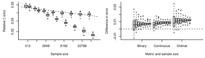
Figure 1: The left plot shows the relative error of the covariance matrix versus the sample size on the log-log scale. The gray boxes are the RQMC method and the white boxes are the AEM method. Regression lines are added on the log-log scale. The right plot shows the difference in mean RMSE and classification error for the three types of data for increasing sample sizes (increasing from left to right). We use the median method for the ordinal outcomes with RQMC as this is the closest to the AEM method.

We now address how our new estimation method and imputation method compare with the AEM based method of Zhao and Udell (2020b), when (i) the model is correctly specified, and (ii) when the methods are applied to observational data. We start with (i). An argument for using the AEM method is that it is fast even when there are moderately many variables (moderately large $K$) and many observations (large $n$). We draw $n=10000$ observations with $K=60$ variables of which $20$ each are continuous, binary, and ordinal. As in Zhao and Udell (2020b), we use five equally likely categories for the ordinal variables and generate $100$ data sets where we mask each variable independently at random with a 30 percent chance. For each data set, we sample $\mathbf{\Sigma}$ from a Wishart distribution with $K$ degrees of freedom with an identity matrix as the scale matrix and scale the sampled matrix such that it is a correlation matrix. Thus, the methods are compared on different correlation matrices. As in Zhao and Udell (2020b), we let the continuous variables have standard exponential (marginal) distributions.

We use three different metrics to measure the performance of the methods. The first two are also used by Zhao and Udell (2020b). The user may be interested in $\mathbf{\Sigma}$ per se and, thus, we use the relative error $\lVert\widehat{\mathbf{\Sigma}}-\mathbf{\Sigma}\rVert_{F}/\lVert\mathbf{\Sigma}\rVert_{F}$, where $\widehat{\mathbf{\Sigma}}$ is an estimated correlation matrix and $\lVert\cdot\rVert_{F}$ is the Frobenius norm. We use the scaled mean absolute error (SMAE) given by $\sum_{i\in\mathcal{H}_{j}}\lVert\widehat{X}_{ij}-X_{ij}\rVert_{1}/\sum_{i\in\mathcal{H}_{j}}\lVert\tilde{X}_{j}-X_{ij}\rVert_{1}$ where $\mathcal{H}_{j}$ is the set of indices with missing entries for variable $j$, $\widehat{X}_{ij}$ is an imputed value, and $\tilde{X}_{j}$ is the median estimate based on the observed values. Finally, we use the classification error for the binary and ordinal variables and the root mean square error (RMSE) for the continuous variables.

Table 1 summaries the results of the simulation study. The RQMC rows are our method which performs imputation by assigning the category with the highest conditional probability. The “Median” rows also use our estimation method but selects the conditional median category similar to the AEM algorithm which back transforms an approximate mean. Our new method performs better on all metrics. Selecting the category with the highest conditional probability leads to a lower classification error but higher SMAE.

The computation time of our method is competitive although we stress that the AEM implementation does not support computation in parallel. Importantly, the average relative error for the correlation matrix is much lower.

Table 2: Mean classification error, RMSE, and SMAEs (see Table 1) with four different data sets used by Zhao and Udell (2020b) and the two largest data sets from the catdata package. The average computation times in seconds are shown in the last column.

Data set	Metric	Method	Binary	Ordinal	Continuous	Time
Rent	Error	RQMC (our)	$0.1212\pm 0.0008$	$0.3702\pm 0.0039$	$0.747\pm 0.004$	$31.67\pm 0.20$
		Median (our)		$0.3710\pm 0.0041$
		AEM (ZU)	$0.1237\pm 0.0008$	$0.3716\pm 0.0039$	$0.746\pm 0.004$	$35.41\pm 0.65$
	SMAE	RQMC (our)	$0.9721\pm 0.0048$	$0.5102\pm 0.0053$	$0.701\pm 0.003$
		Median (our)		$0.5095\pm 0.0054$
		AEM (ZU)	$0.9974\pm 0.0016$	$0.5107\pm 0.0052$	$0.706\pm 0.002$
Medcare	Error	RQMC (our)	$0.3418\pm 0.0016$	$0.4398\pm 0.0010$	$0.984\pm 0.006$	$6.74\pm 0.27$
		Median (our)		$0.4661\pm 0.0010$
		AEM (ZU)	$0.3466\pm 0.0017$	$0.4647\pm 0.0010$	$0.987\pm 0.006$	$22.63\pm 0.11$
	SMAE	RQMC (our)	$0.8020\pm 0.0046$	$0.9823\pm 0.0011$	$0.951\pm 0.001$
		Median (our)		$0.9639\pm 0.0013$
		AEM (ZU)	$0.8138\pm 0.0038$	$0.9641\pm 0.0010$	$0.952\pm 0.001$
ESL	Error	RQMC (our)		$0.4911\pm 0.0036$		$1.80\pm 0.31$
		Median (our)		$0.4908\pm 0.0036$
		AEM (ZU)		$0.4919\pm 0.0035$		$2.05\pm 0.04$
	SMAE	RQMC (our)		$0.5309\pm 0.0053$
		Median (our)		$0.5238\pm 0.0053$
		AEM (ZU)		$0.5254\pm 0.0052$
LEV	Error	RQMC (our)		$0.6337\pm 0.0023$		$2.20\pm 0.33$
		Median (our)		$0.6476\pm 0.0021$
		AEM (ZU)		$0.6484\pm 0.0021$		$5.40\pm 0.07$
	SMAE	RQMC (our)		$0.9637\pm 0.0067$
		Median (our)		$0.8696\pm 0.0028$
		AEM (ZU)		$0.8714\pm 0.0027$
GBSG	Error	RQMC (our)	$0.2895\pm 0.0031$	$0.3610\pm 0.0044$	$0.921\pm 0.008$	$2.64\pm 0.35$
		Median (our)		$0.3604\pm 0.0044$
		AEM (ZU)	$0.2889\pm 0.0031$	$0.3572\pm 0.0046$	$0.925\pm 0.008$	$7.13\pm 0.15$
	SMAE	RQMC (our)	$0.7276\pm 0.0084$	$1.0207\pm 0.0060$	$0.879\pm 0.003$
		Median (our)		$1.0189\pm 0.0061$
		AEM (ZU)	$0.7257\pm 0.0082$	$1.0085\pm 0.0041$	$0.878\pm 0.002$
TIPS	Error	RQMC (our)	$0.2857\pm 0.0058$	$0.4133\pm 0.0072$	$0.786\pm 0.016$	$1.67\pm 0.17$
		Median (our)		$0.4414\pm 0.0088$
		AEM (ZU)	$0.2874\pm 0.0062$	$0.4489\pm 0.0091$	$0.784\pm 0.016$	$1.56\pm 0.04$
	SMAE	RQMC (our)	$0.8241\pm 0.0142$	$0.8007\pm 0.0174$	$0.763\pm 0.008$
		Median (our)		$0.7786\pm 0.0154$
		AEM (ZU)	$0.8284\pm 0.0139$	$0.7881\pm 0.0155$	$0.761\pm 0.008$

For our second evaluation, we compare the methods on six data sets. We use four of the data sets where Zhao and Udell (2020b) show that the AEM method yields superior single imputation performance compared to state of the art non-parametric methods. These are the lecturers evaluation (LEV) data set, employee selection (ESL) data set, German breast cancer study group (GBSG) data set, and restaurant tips (TIPS). We also add the two largest data sets from the catdata package (Fox et al., 2020). This is the medcare data set containing the number of physician office visits and the rent in Munich data set. Both data sets have variables of all types (binary, ordinal, and continuous). We generate $100$ data sets for each of the six where we independently at random mask each variable with a 30 percent chance and standardize all continuous variables such that the RMSE is not dominated by a few variables. The first four data sets have between $244$ and $1000$ observations while the latter two have $2053$ and $4406$ observations. Further details about all data sets in this paper can be found in supplementary material S5.

Table 2 summarises the results. With respect to the standard errors there are only noticeable differences in the average errors for the two larger data sets where our method is preferred. A reason for there seemingly being no differences for the smaller data sets can be that the AEM method tends to select a correlation matrix close to a diagonal matrix. The average differences between the Frobenius norm of the estimated correlation matrix of the two methods ranged from $0.0123$ to $0.691$ over the six data sets. This might lead to bias-variance trade-off.

To explore this further, we have conducted a new simulation study with $K=15$ variables and $5$ of each type of outcome to reduce the computation time. We use $n=512,1024,\dots,65536$ observations with 50 data sets for each $n$. The results are summarized in Figure 1 which shows that the AEM method does not improve in terms of the relative error of the estimated covariance matrix (or at best very slowly) for large sample sizes. This makes it hard to believe that the AEM method will converge, which implies that it must be biased for some sample sizes. This is troubling if the researcher is interested in the covariance matrix, as in Figure 6 in Zhao and Udell (2020c). In contrast, our proposed method has a regression slope of -0.5006 consistent with the typical $\sqrt{n}$ convergence rate of maximum likelihood estimators. Figure 1 also shows that the gap in imputation error increases as a function of the sample size.

To summarize, we find large improvements when the model is correctly specified and only improvements or identical results with observational data sets. There is a big difference in the average error for the estimated correlation matrix for the correctly specified model which is very important for researchers who are interested in the correlation matrix per se. Importantly, the differences in the error of the two methods increases as the number of samples increase which is consistent with the observational data. This suggests that the RQMC is preferable when there are many observations.

5 Adding Multinomial Variables

We extend the model in this section to also support multinomial variables. To build up the intuition, we first show the formulation with a simple model with one binary variable $X_{1}\in\{0,1\}$ and one continuous variable $X_{2}$. Suppose that

$$\bm{Z} \sim N^{(3)}\left(\begin{pmatrix}0\\ \mu_{2}\\ 0\end{pmatrix},\begin{pmatrix}\xi&0&0\\ 0&1&\sigma_{23}\\ 0&\sigma_{32}&1\end{pmatrix}\right)$$ (6)

$$X_{1} =j-1\Leftrightarrow Z_{j}\geq\max(Z_{1},Z_{2})\qquad j\in\{1,2\}$$ (7)

$$X_{2} =f(Z_{3})$$

for a bijective function $f$ and $\mu_{2}=\Phi^{-1}(p_{1})$. Using that $\bm{Z}_{1:2}\mid Z_{3}=z\sim N(\bm{m},\mathbf{S})$ with $\bm{m}=(0,\mu_{2}+\sigma_{23}z)^{\top}$ and

$$\mathbf{S}=\begin{pmatrix}\xi&0\\ 0&1-\sigma_{23}^{2}\end{pmatrix},$$

we get

$$\operatorname{P}(X_{1}=1\mid Z_{3}=z) =\int\phi(u;m_{2},s_{22})\Phi\left(u;0,\xi\right)\operatorname{d\!}{}u$$

$$=\Phi(0;-m_{2},\xi+s_{22})=\Phi\left(\frac{\mu_{2}+\sigma_{23}z}{\sqrt{1+\xi-\sigma_{23}^{2}}}\right)$$

where the result is attained using the identity in supplementary material S1. This is the Gaussian copula model we have been working with if we let $\xi\rightarrow 0^{+}$ which effectively means that $Z_{1}=0$. In practice, we derive the formulas we need and work with $\xi=0$ and we only work with one latent variable for binary variables as Zhao and Udell (2020b).

Now, consider the extension to the scenario with one multinomial variable $X_{1}\in\{0,\cdots,G-1\}$, and $L$ continuous variables. Assume that $\bm{Z}\sim N^{(L+G)}(\bm{\mu},\mathbf{\Psi}$) where

$$\mathbf{\Psi} =\begin{pmatrix}\xi&\bm{0}^{\top}_{G-1}&\bm{0}^{\top}_{L}\\ \bm{0}_{G-1}&\mathbf{\Psi}_{2:G2:G}&\mathbf{\Psi}_{2:G(-1:G)}\\ \bm{0}_{L}&\mathbf{\Psi}_{(-1:G)2:G}&\mathbf{\Psi}_{(-1:G)(-1:G)}\end{pmatrix}$$

$$\mathbf{\Psi}_{2:G2:G} =\begin{pmatrix}1&\sigma_{23}&\cdots&\sigma_{2K}\\ \sigma_{32}&\sigma_{33}&\ddots&\sigma_{3G}\\ \vdots&\ddots&\ddots&\vdots\\ \sigma_{G2}&\sigma_{G3}&\dots&\sigma_{GG}\end{pmatrix}$$

$$X_{1} =j-1\Leftrightarrow Z_{j}\geq\max(Z_{1},\dots,Z_{G})$$

$$\bm{X}_{(-1)} =\bm{f}^{-1}(\bm{Z}_{(-1:G)}),$$

$j\in\{1,\dots,G\}$, $\bm{\mu}=(0,\bm{\mu}_{2:G}^{\top},\bm{0}_{L}^{\top})^{\top}$, $\mathbf{\Psi}_{(-1:G)2:G}\in\mathbb{R}^{L\times(G-1)}$ is a dense matrix, and $\mathbf{\Psi}_{(-1:G)(-1:G)}\in\mathbb{R}^{L\times L}$ is a matrix in which diagonal entries are restricted to be one. This parameterization is used by Bunch (1991), in the absence of the continuous variables. We have $G$ conditional probabilities given by

$$\operatorname{P}(X_{1}=j-1\mid\bm{Z}_{(-1:G)}=\bm{z})=\int\phi(u;m_{j},s_{jj})\Phi^{(G-1)}\bigg{(}\\ \bm{1}_{G-1}u;\big{(}\bm{m}_{(-j)}+\mathbf{S}_{(-j)j}\frac{u-m_{j}}{s_{jj}}\big{)},\big{(}\mathbf{S}_{(-j)(-j)}-s_{jj}^{-1}\mathbf{S}_{(-j)j}\mathbf{S}_{j(-j)}\big{)}\bigg{)}\operatorname{d\!}{}u$$

which equals

$$\Phi^{(G-1)}\bigg{(}\bm{0}_{G-1};\bm{m}_{(-j)}-\bm{1}_{G-1}m_{j},\mathbf{S}_{(-j)(-j)}+s_{jj}\bm{1}_{G-1}\bm{1}_{G-1}^{\top}-\bm{1}_{G-1}\mathbf{S}_{j(-j)}-\mathbf{S}_{(-j)j}\bm{1}_{G-1}^{\top}\bigg{)}$$

where $\bm{Z}_{1:G}\mid\bm{Z}_{(-1:G)}=\bm{z}\sim N(\bm{m},\mathbf{S})$,

$$\bm{m} =\bm{\mu}_{1:G}+\mathbf{\Sigma}_{1:G(-1:G)}\mathbf{\Sigma}_{(-1:G)(-1:G)}^{-1}\bm{z}$$

$$\mathbf{S} =\mathbf{\Sigma}_{1:G,1:G}-\mathbf{\Sigma}_{1:G(-1:G)}\mathbf{\Sigma}_{(-1:G)(-1:G)}^{-1}\mathbf{\Sigma}_{(-1:G)1:G},$$

$\bm{1}_{k}$ is a vector with $k$ ones, and $(-j)$ or $(-\mathcal{J})$ in a subscript implies all elements but the $j^{\text{th}}$ or those indices in $\mathcal{J}$ for vectors or all but those indices in the rows or columns for matrices.

5.1 New Log Marginal Likelihood

We can now turn to the general case with all types including multiple multinomial variables and show the log marginal likelihood term for each of the $n$ observations. Suppose that the entries $X_{ij}$ with $j\in\mathcal{M}\subseteq\{1,\dots,K\}$ are multinomial variables with $\mathcal{M}\cap\mathcal{C}=\emptyset$, $\mathcal{M}\cap\mathcal{O}=\emptyset$, and $\mathcal{B}=\{1,\dots,K\}\setminus\mathcal{C}\cup\mathcal{O}\cup\mathcal{M}$. Each variable $X_{ij}\in\{0,1,\dots m_{j}-1\}$ has $m_{j}$ categories when $j\in\mathcal{M}$. We permute the the observed variables, the $\bm{X}_{i}$’s, such that the multinomial variables are first without loss of generality and let $c_{\mathcal{M}}=\lvert\mathcal{M}\rvert$ and $c_{\setminus\mathcal{M}}=K-c_{\mathcal{M}}$. The model is then $\bm{Z}_{i}\sim N^{(W)}\left(\bm{\mu},\mathbf{\Psi}\right)$ where $W=c_{\setminus\mathcal{M}}+\sum_{j=1}^{c_{\mathcal{M}}}m_{j}$, $\mathbf{\Psi}$ is given in supplementary material S2, and $\lvert\mathcal{B}\rvert+\sum_{j=1}^{c_{\mathcal{M}}}m_{j}-c_{\mathcal{M}}$ entries of $\bm{\mu}$ are non-zero. One can permute $\mathbf{\Psi}$ with a permutation matrix $\mathbf{P}$ such that:

$$\mathbf{P}\mathbf{\Psi}\mathbf{P}^{\top}=\begin{pmatrix}\xi\mathbf{I}_{c_{\mathcal{M}}}&\mathbf{0}_{c_{\mathcal{M}}\times(W-c_{\mathcal{M}})}\\ \mathbf{0}_{(W-c_{\mathcal{M}})\times c_{\mathcal{M}}}&\mathbf{\Sigma}\end{pmatrix}$$ (8)

where $\mathbf{I}_{k}$ is the $k$ dimensional identity matrix, $\mathbf{0}_{k\times l}$ is a $k\times l$ matrix with zeros, and $\mathbf{\Sigma}$ is a symmetric positive definite matrix where all elements are free except for $K$ of the diagonal entries which are restricted to be one. Thus, we parameterize $\mathbf{\Psi}$ in terms of a log Cholesky decomposition of $\mathbf{\Sigma}$. As before, the restriction in the diagonal of $\mathbf{\Sigma}$ is either applied after each stochastic gradient iteration by scaling the rows and columns, similar to what Zhao and Udell (2020b) do, or by using a constrained nonlinear optimization method.

We now turn to the new expression of the log marginal likelihood. Let

$$\mathbf{D}=\begin{pmatrix}\bm{1}_{m_{1}-1}&\bm{0}_{m_{1}-1}&\cdots&\bm{0}_{m_{1}-1}\\ \bm{0}_{m_{2}-1}&\bm{1}_{m_{2}-1}&\ddots&\vdots\\ \vdots&\ddots&\ddots&\bm{0}_{m_{c_{\mathcal{M}}-1}-1}\\ \bm{0}_{m_{c_{\mathcal{M}}}-1}&\dots&\bm{0}_{m_{c_{\mathcal{M}}}-1}&\bm{1}_{m_{c_{\mathcal{M}}}-1}\\ \bm{0}_{\lvert\mathcal{O}\cup\mathcal{B}\rvert}&\cdot&\bm{0}_{\lvert\mathcal{O}\cup\mathcal{B}\rvert}&\bm{0}_{\lvert\mathcal{O}\cup\mathcal{B}\rvert}\end{pmatrix}.$$

Furthermore, we let $\mathcal{I}_{i}$ be the set with the indices of the latent variables belonging to each of the observed categories for the multinomial variables for observation $i$. That is

$$\mathcal{I}_{i}=\left\{k=1,\dots,c_{\mathcal{M}}:\,X_{ik}+1+\sum_{l=1}^{k-1}m_{l}\right\}$$

where $\sum_{l=1}^{0}m_{l}=0$ by definition.

Let $\tilde{\mathcal{C}}$ be the indices of the latent variables corresponding to the observed continuous variables and similarly define $\tilde{\mathcal{O}}$, $\tilde{\mathcal{B}}$, and $\tilde{\mathcal{M}}$. Using

$$\bar{\bm{\mu}} =\bm{\mu}_{\tilde{\mathcal{B}}\cup\tilde{\mathcal{O}}\cup\tilde{\mathcal{M}}}+\mathbf{\Psi}_{\tilde{\mathcal{B}}\cup\tilde{\mathcal{O}}\cup\tilde{\mathcal{M}},\tilde{\mathcal{C}}}\mathbf{\Psi}_{\tilde{\mathcal{C}}\tilde{\mathcal{C}}}^{-1}\widehat{\bm{z}}_{i\tilde{\mathcal{C}}}$$ (9)

$$\bar{\mathbf{S}} =\mathbf{\Psi}_{\tilde{\mathcal{B}}\cup\tilde{\mathcal{O}}\cup\tilde{\mathcal{M}},\tilde{\mathcal{B}}\cup\tilde{\mathcal{O}}\cup\tilde{\mathcal{M}}}-\mathbf{\Psi}_{\tilde{\mathcal{B}}\cup\tilde{\mathcal{O}}\cup\tilde{\mathcal{M}},\tilde{\mathcal{C}}}\mathbf{\Psi}_{\tilde{\mathcal{C}},\tilde{\mathcal{C}}}^{-1}\mathbf{\Psi}_{\tilde{\mathcal{C}},\tilde{\mathcal{B}}\cup\tilde{\mathcal{O}}\cup\tilde{\mathcal{M}}},$$ (10)

we can apply the identity in supplementary material S1 to get the following log marginal likelihood expression

$$l_{i}(\mathbf{\Psi},\bm{\mu}) =\log\phi^{(\lvert\mathcal{C}\rvert)}(\widehat{\bm{z}}_{i\tilde{\mathcal{C}}};\bm{0},\mathbf{\Psi}_{\tilde{\mathcal{C}}\tilde{\mathcal{C}}})+\log\int\phi^{(c_{\mathcal{M}})}(\bm{u};\bar{\bm{\mu}}_{\mathcal{I}_{i}},\bar{\mathbf{S}}_{\mathcal{I}_{i}\mathcal{I}_{i}})\Phi^{(W)}\Big{(}\bm{a}_{i},\bm{b}_{i};$$ (11)

$$\big{(}\bar{\bm{\mu}}_{(-\mathcal{I}_{i})}-\mathbf{D}\bm{u}+\mathbf{S}_{(-\mathcal{I}_{i})\mathcal{I}_{i}}\bar{\mathbf{S}}_{\mathcal{I}_{i}\mathcal{I}_{i}}^{-1}(\bm{u}-\bar{\bm{\mu}}_{\mathcal{I}_{i}})\big{)},\big{(}\bar{\mathbf{S}}_{(-\mathcal{I}_{i})(-\mathcal{I}_{i})}-\bar{\mathbf{S}}_{(-\mathcal{I}_{i})\mathcal{I}_{i}}\bar{\mathbf{S}}_{\mathcal{I}_{i}\mathcal{I}_{i}}^{-1}\bar{\mathbf{S}}_{\mathcal{I}_{i}(-\mathcal{I}_{i})}\big{)}\Big{)}\operatorname{d\!}{}\bm{u}$$

$$=\log\phi^{(\lvert\mathcal{C}\rvert)}(\widehat{\bm{z}}_{i\mathcal{C}};\bm{0},\mathbf{\Psi}_{\tilde{\mathcal{C}}\tilde{\mathcal{C}}})+\log\Phi^{(W)}\Big{(}$$

$$\bm{a}_{i},\bm{b}_{i};\big{(}\bar{\bm{\mu}}_{(-\mathcal{I}_{i})}-\mathbf{D}\bar{\bm{\mu}}_{\mathcal{I}_{i}}\big{)},\big{(}\bar{\mathbf{S}}_{(-\mathcal{I}_{i})(-\mathcal{I}_{i})}+\mathbf{D}\bar{\mathbf{S}}_{\mathcal{I}_{i}\mathcal{I}_{i}}\mathbf{D}^{\top}-\mathbf{D}\bar{\mathbf{S}}_{\mathcal{I}_{i}(-\mathcal{I}_{i})}-\bar{\mathbf{S}}_{(-\mathcal{I}_{i})\mathcal{I}_{i}}\mathbf{D}^{\top}\big{)}\Big{)}.$$

A missing $X_{ij}$ implies that the corresponding $\bm{Z}_{i}$ entry or entries are unrestricted. Thus, they do not contribute anything to the log marginal likelihood in Equation (3) and (11) after integrating them out and can be omitted. Notice that the non-zero mean terms, some of the terms of $\bm{\mu}_{\tilde{\mathcal{B}}\cup\tilde{\mathcal{O}}\cup\tilde{\mathcal{M}}}$, enter linearly in Equation (9). This makes it easy to jointly optimize the mean and covariance matrix, rather then fixing the mean as suggested by Zhao and Udell (2020b), as we have a gradient approximation of the mean of the CDF. Thus, we can easily estimate the mean vector for the binary and multinomial variables together with $\mathbf{\Sigma}$.

5.2 Application

We compare our method with other top performing single imputation methods in this section. The methods we compare with are missForest and the PCA-like imputeFAMD. We are particularly interested in (i) the improvements from using our method for a correctly specified model and (ii) the performance of all three methods on observational data. We start with (i) which will give an indication of the improvements we may expect when the data generating process is approximately a Gaussian copula.

Table 3: Average RMSE and classification errors on simulated data sets and three observational data sets. The average computation times in seconds are given in the last column.

Data set	Method	Binary	Ordinal	Continuous	Multinomial	Time
Simulation	RQMC (our)	$0.3051\pm 0.0064$	$0.647\pm 0.006$	$0.883\pm 0.013$	$0.535\pm 0.005$	$47.05\pm 0.99$
	missForest	$0.3451\pm 0.0065$	$0.692\pm 0.006$	$0.949\pm 0.011$	$0.603\pm 0.006$	$8.72\pm 0.25$
	imputeFAMD	$0.3573\pm 0.0074$	$0.701\pm 0.006$	$0.929\pm 0.011$	$0.613\pm 0.007$	$81.19\pm 0.38$
Cholesterol	RQMC (our)	$0.3009\pm 0.0012$	$0.679\pm 0.002$		$0.538\pm 0.002$	$10.64\pm 0.83$
	missForest	$0.4022\pm 0.0046$	$0.696\pm 0.003$		$0.700\pm 0.008$	$2.88\pm 0.12$
	imputeFAMD	$0.2994\pm 0.0011$	$0.691\pm 0.002$		$0.564\pm 0.003$	$5.61\pm 0.27$
Rent	RQMC (our)	$0.1096\pm 0.0007$	$0.370\pm 0.004$	$0.731\pm 0.003$	$0.890\pm 0.002$	$173.55\pm 0.54$
	missForest	$0.1408\pm 0.0009$	$0.389\pm 0.004$	$0.757\pm 0.004$	$0.903\pm 0.002$	$19.07\pm 0.70$
	imputeFAMD	$0.1121\pm 0.0008$	$0.537\pm 0.005$	$0.777\pm 0.003$	$0.959\pm 0.002$	$102.97\pm 2.24$
Colon	RQMC (our)	$0.2217\pm 0.0014$	$0.223\pm 0.002$	$1.029\pm 0.008$	$0.659\pm 0.004$	$28.73\pm 0.91$
	missForest	$0.2666\pm 0.0025$	$0.394\pm 0.005$	$1.060\pm 0.007$	$0.614\pm 0.004$	$11.50\pm 0.44$
	imputeFAMD	$0.2275\pm 0.0014$	$0.223\pm 0.002$	$1.017\pm 0.007$	$0.671\pm 0.004$	$51.42\pm 0.98$

For (i) and (ii) we generate $100$ data sets and within each there is a 30 percent chance that a variable is missing (missing independently at random). The imputeFAMD has a tuning parameter which is the number of components. We estimate this using five-fold cross validation. In our simulation study (i) we simulate data from a Gaussian copula in a similar manner to that described in Section 4.1. That is, we simulate $\mathbf{\Sigma}$ in $\mathbf{\Psi}$ in Equation (8) from a Wishart distribution like in the previous simulation. We have $8$ variables per observation with $2$ of each type. The ordinal and multinomial variables have five equally likely categories and there is a total 2000 observations.

The result of the simulation study is shown in the “Simulation” rows in Table 3. Our method performs much better for all four types of variables. The average computation times for the simulated and observational data show that our method is the slowest of the three. However, it is not orders of magnitude slower.

We include three observational data sets: the rent data set, used also in Section 4.1, but this time with the multinomial area code, the cholesterol data from a US survey from the survey package (Lumley, 2020), and data from one of the first successful trials of adjuvant chemotherapy for colon cancer from the survival package (Therneau, 2020). Our method often performs best or is close to the best performing method. It is expected that our method is not always the best performing method as we do make a parametric assumption with the particular copula we use. It is, however, encouraging that the data generating processes seem well approximated with the Gaussian copula for all three data sets.

6 Conclusion and Discussion

We have shown that direct maximum likelihood estimation of the model used by Zhao and Udell (2020b, a) using RQMC is feasible and provides improvements compared with the approximation that they use. Our RQMC method yielded lower errors for the imputed values, and estimated model parameters closer to the true values in our simulation study. Importantly, the error of our method decreases faster as a function of the number of samples. We have also extended the model to support multinomial variables which increases the applicability of the method.

6.1 Future Work

Our RQMC method can be extended to provide e.g. an arbitrarily precise approximation of the quantiles of the latent variables conditional on the observed data and estimated model parameters. A major advantage of having precise quantile approximations is that the user can get a quantile estimate at a given level which is close to the nominal level if the data generating process is well approximated by the Gaussian copula. These may provide substantial improvements over the lower bounds and approximate confidence intervals based on Gaussian approximations, that Zhao and Udell (2020a) suggest using, since the conditional distribution of the latent variables may be very non-Gaussian.

We could replace the non-parametric density estimator with a flexible parametric transformation like those used in transformation models Hothorn et al. (2018). This would lead to a fully parametric model for which it would be possible to do joint optimization over all parameters, including the borders for the ordinal variables. This could substantially increase the efficiency and subsequently the performance. Our RQMC could be extended to use the recently developed minimax tilting method by Botev (2017) which could decrease the computation time at a fixed variance of the estimator. Finally, our method can easily be used for multiple imputation (to, importantly, account for imputation uncertainty), since it is a probabilistic framework.

S1 Multivariate Normal CDF Identity

In this section, we show an identity which we will use repeatably. Let

$$\begin{pmatrix}\bm{V}_{1}\\ \bm{V}_{2}\end{pmatrix}\sim N^{(k_{1}+k_{2})}\left(\begin{pmatrix}\bm{\xi}_{1}\\ \bm{\xi}_{2}\end{pmatrix},\begin{pmatrix}\mathbf{\Xi}_{11}&\mathbf{\Xi}_{12}\\ \mathbf{\Xi}_{21}&\mathbf{\Xi}_{22}\end{pmatrix}\right)$$

where $\bm{V}_{1}\in\mathbb{R}^{k_{1}}$ and $\bm{V}_{2}\in\mathbb{R}^{k_{2}}$, $\bm{\xi}_{1}$ and $\bm{\xi}_{2}$ are mean vectors for $\bm{V}_{1}$ and $\bm{V}_{2}$, respectively, and $\mathbf{\Xi}$ is a covariance matrix where the sub matrices have $k_{1}$ or $k_{2}$ rows and columns. Then the joint density of $\bm{V}_{1}=\bm{v}_{1}$ and $\bm{a}<\bm{V}_{2}<\bm{b}$ (a box constraint on $\bm{V}_{2}$) is

$$\phi^{(k_{1})}(\bm{v}_{1};\bm{\xi}_{1},\mathbf{\Xi}_{11})\operatorname{P}\left(\bm{a}<\bm{V}_{2}<\bm{b}\,\middle|\,\bm{V}_{1}=\bm{v}_{1}\right)$$

$$=\phi^{(k_{1})}(\bm{v}_{1};\bm{\xi}_{1},\mathbf{\Xi}_{11})\Phi^{(k_{2})}\bigg{(}\bm{a},\bm{b};\big{(}\bm{\xi}_{2}+\mathbf{\Xi}_{21}\mathbf{\Xi}_{11}^{-1}(\bm{v}_{1}-\bm{\xi}_{1})\big{)},\big{(}\mathbf{\Xi}_{22}-\mathbf{\Xi}_{21}\mathbf{\Xi}_{11}^{-1}\mathbf{\Xi}_{12}\big{)}\bigg{)}$$

and the marginal for $\operatorname{P}(\bm{a}<\bm{V}_{2}<\bm{b})$ is

$$\operatorname{P}(\bm{a}<\bm{V}_{2}<\bm{b})$$

$$=\Phi^{(k_{2})}(\bm{a},\bm{b};\bm{\xi}_{2},\mathbf{\Xi}_{22})$$

$$=\int\phi^{(k_{1})}(\bm{v}_{1};\bm{\xi}_{1},\mathbf{\Xi}_{11})\operatorname{P}\left(\bm{a}<\bm{V}_{2}<\bm{b}\,\middle|\,\bm{V}_{1}=\bm{v}_{1}\right)\operatorname{d\!}{}\bm{v}_{1}.$$

Next, we can define

$$\mathbf{Z} =\mathbf{\Xi}_{21}\mathbf{\Xi}_{11}^{-1}$$

$$\bm{c} =\bm{\xi}_{2}-\mathbf{\Xi}_{21}\mathbf{\Xi}_{11}^{-1}\bm{\xi}_{1}=\bm{\xi}_{2}-\mathbf{Z}\bm{\xi}_{1}$$

$$\mathbf{\Omega} =\mathbf{\Xi}_{22}-\mathbf{\Xi}_{21}\mathbf{\Xi}_{11}^{-1}\mathbf{\Xi}_{12}=\mathbf{\Xi}_{22}-\mathbf{Z}\mathbf{\Xi}_{11}\mathbf{Z}^{\top}$$

which we can use to show that

$$\int\phi^{(k_{1})}(\bm{x};\bm{\mu},\mathbf{\Sigma})\Phi^{(k_{2})}(\bm{a},\bm{b};\bm{c}+\mathbf{Z}\bm{x},\mathbf{\Omega})\operatorname{d\!}{}\bm{x}=\Phi^{(k_{2})}(\bm{a},\bm{b};\bm{c}+\mathbf{Z}\bm{\mu},\mathbf{\Omega}+\mathbf{Z}\mathbf{\Sigma}\mathbf{Z}^{\top}).$$ (12)

S2 Parameterization for the General Model with More than One Multinomial Variable

Following the notation in Section 5.1, we can generalize the covariance matrix for $\bm{Z}$ in Section 5 to include all variable types including multiple multinomial variables by letting $\mathbf{\Psi}$ be:

$$\mathbf{\Psi} =\begin{pmatrix}\mathbf{\Psi}^{(11)}&\cdots&\mathbf{\Psi}^{(1l)}\\ \vdots&\ddots&\vdots\\ \mathbf{\Psi}^{(l1)}&\dots&\mathbf{\Psi}^{(ll)}\end{pmatrix}$$

$$\mathbf{\Psi}^{(kk)} =\begin{pmatrix}\xi&0&0&\cdots&0\\ 0&1&\psi^{(kk)}_{23}&\cdots&\psi^{(kk)}_{2m_{k}}\\ 0&\psi^{(kk)}_{32}&\psi^{(kk)}_{33}&\ddots&\psi^{(kk)}_{3m_{k}}\\ \vdots&\vdots&\ddots&\ddots&\vdots\\ 0&\psi^{(kk)}_{m_{k}2}&\psi^{(kk)}_{m_{k}3}&\dots&\psi^{(kk)}_{m_{k}m_{k}}\end{pmatrix}$$

$$\mathbf{\Psi}^{(kk^{\prime})} =\begin{pmatrix}0&0&\cdots&0\\ 0&\psi^{(kk^{\prime})}_{22}&\cdots&\psi^{(kk^{\prime})}_{2m_{k^{\prime}}}\\ \vdots&\vdots&\ddots&\vdots\\ 0&\psi^{(kk^{\prime})}_{m_{k}2}&\dots&\psi^{(kk^{\prime})}_{m_{k}m_{k^{\prime}}}\end{pmatrix}$$

$$\mathbf{\Psi}^{(kl)} =\begin{pmatrix}0&\cdots&0\\ \psi^{(kl)}_{21}&\cdots&\psi^{(kl)}_{2c_{\setminus\mathcal{M}}}\\ \vdots&\ddots&\vdots\\ \psi^{(kl)}_{m_{k}1}&\cdots&\psi^{(kl)}_{m_{k}c_{\setminus\mathcal{M}}}\end{pmatrix}$$

$$\mathbf{\Psi}^{(ll)} =$$

$$\begin{pmatrix}1&\psi^{(ll)}_{12}&\cdots&\psi^{(ll)}_{1c_{\setminus\mathcal{M}}}\\ \psi^{(ll)}_{21}&1&\ddots&\vdots\\ \vdots&\ddots&\ddots&\psi^{(ll)}_{c_{\setminus\mathcal{M}}-1,c_{\setminus\mathcal{M}}}\\ \psi^{(ll)}_{c_{\setminus\mathcal{M}}1}&\dots&\psi^{(ll)}_{c_{\setminus\mathcal{M}},c_{\setminus\mathcal{M}}-1}&1\end{pmatrix}$$

for $k,k^{\prime}\in\{1,\dots,c_{\mathcal{M}}\}\wedge k^{\prime}\neq k$ and $l=c_{\mathcal{M}}+1$. The $k^{\text{th}}$ $\mathbf{\Psi}^{(kk)}$ in the diagonal for $k=1,\dots,c_{\mathcal{M}}$ is for the latent variables for the $k^{\text{th}}$ multinomial variable. The last $\mathbf{\Psi}^{(ll)}$ block is for the latent variables for the binary, continuous, and ordinal variables.

S3 Derivative Approximations

We show the gradient of the log marginal likelihood with respect to the covariance matrix, $\mathbf{\Psi}$, in this section. Without loss of generality, suppose that covariance matrix $\mathbf{\Psi}$ is permutated such that the first indices are for the latent variables for the continuous variables, the next $\lvert\mathcal{M}\rvert$ indices are the latent variables corresponding to the observed categories of the multinomial variables, and the final indices are the remaining latent variables for the multinomial, ordinal, and binary variables. That is,

$$\mathcal{R}_{i} =\tilde{\mathcal{M}}\cup\tilde{\mathcal{O}}\cup\tilde{\mathcal{B}}\setminus\mathcal{I}_{i}$$

$$\mathbf{\Psi} =\begin{pmatrix}\mathbf{\Psi}_{\mathcal{C}\mathcal{C}}&\mathbf{\Psi}_{\mathcal{C}\mathcal{I}_{i}}&\mathbf{\Psi}_{\mathcal{C}\mathcal{R}_{i}}\\ \mathbf{\Psi}_{\mathcal{I}_{i}\mathcal{C}}&\mathbf{\Psi}_{\mathcal{I}_{i}\mathcal{I}_{i}}&\mathbf{\Psi}_{\mathcal{I}_{i}\mathcal{R}_{i}}\\ \mathbf{\Psi}_{\mathcal{R}_{i}\mathcal{C}}&\mathbf{\Psi}_{\mathcal{R}_{i}\mathcal{I}_{i}}&\mathbf{\Psi}_{\mathcal{R}_{i}\mathcal{R}_{i}}\end{pmatrix}$$

$$\bar{\bm{\mu}} =(\bar{\bm{\mu}}_{1:c_{\mathcal{M}}},\bar{\bm{\mu}}_{(-1:c_{\mathcal{M}})})^{\top}$$

$$\bar{\mathbf{S}} =\begin{pmatrix}\bar{\mathbf{S}}_{1:c_{\mathcal{M}}1:c_{\mathcal{M}}}&\bar{\mathbf{S}}_{1:c_{\mathcal{M}}(-1:c_{\mathcal{M}})}\\ \bar{\mathbf{S}}_{(-1:c_{\mathcal{M}})1:c_{\mathcal{M}}}&\bar{\mathbf{S}}_{(-1:c_{\mathcal{M}})(-1:c_{\mathcal{M}})}\end{pmatrix}$$

where $\bar{\bm{\mu}}$ and $\bar{\mathbf{S}}$ are given in Equation (9) and (10). It follows that the log marginal likelihood in Equation (11) is

$$l_{i} =\log\phi^{(\lvert\mathcal{C}\rvert)}(\widehat{\bm{z}}_{i\mathcal{C}};\bm{0},\mathbf{\Psi}_{\mathcal{C}\mathcal{C}})\log\Phi^{(c_{\setminus\mathcal{M}}+\sum_{j=1}^{c_{\mathcal{M}}}(m_{j}-1))}\left(\bm{a}_{i},\bm{b}_{i};\bm{m},\mathbf{M}\right)$$

$$\bm{m} =\bar{\bm{\mu}}_{(-1:c_{\mathcal{M}})}-\mathbf{D}\bar{\bm{\mu}}_{1:c_{\mathcal{M}}}$$

$$\mathbf{M} =\bar{\mathbf{S}}_{(-1:c_{\mathcal{M}})(-1:c_{\mathcal{M}})}+\mathbf{D}\bar{\mathbf{S}}_{1:c_{\mathcal{M}}1:c_{\mathcal{M}}}\mathbf{D}^{\top}-\mathbf{D}\bar{\mathbf{S}}_{1:c_{\mathcal{M}}(-1:c_{\mathcal{M}})}-\bar{\mathbf{S}}_{(-1:c_{\mathcal{M}})1:c_{\mathcal{M}}}\mathbf{D}^{\top}.$$

For a matrix $\mathbf{A}\in\mathbb{R}^{g\times g}$, we let

$$\mathbf{A}^{\prime}=\begin{pmatrix}\partial l_{i}/\partial a_{11}&\cdots&\partial l_{i}/\partial a_{1g}\\ \vdots&\ddots&\vdots\\ \partial l_{i}/\partial a_{g1}&\dots&\partial l_{i}/\partial a_{gg}\end{pmatrix}.$$

It then follows that

$$\bar{\mathbf{S}}^{\prime} =\begin{pmatrix}\mathbf{D}^{\top}\mathbf{M}^{\prime}\mathbf{D}&-\mathbf{D}^{\top}\mathbf{M}^{\prime}\\ -\mathbf{M}^{\prime}\mathbf{D}&\mathbf{M}^{\prime}\end{pmatrix}$$

$$\mathbf{\Psi}_{\mathcal{I}_{i}\cup\mathcal{R}_{i},\mathcal{I}_{i}\cup\mathcal{R}_{i}}^{\prime} =\bar{\mathbf{S}}^{\prime}$$

$$\bar{\bm{\mu}}^{\prime} =\begin{pmatrix}\mathbf{D}^{\top}\bm{m}^{\prime}\\ \bm{m}^{\prime}\end{pmatrix}$$

$$\mathbf{\Psi}_{\mathcal{C}\mathcal{C}}^{\prime} =\mathbf{\Psi}_{\mathcal{C}\mathcal{C}}^{-1}\mathbf{\Psi}_{\mathcal{C},\mathcal{I}_{i}\cup\mathcal{R}_{i}}\bar{\mathbf{S}}^{\prime}\mathbf{\Psi}_{\mathcal{I}_{i}\cup\mathcal{R}_{i},\mathcal{C}}\mathbf{\Psi}_{\mathcal{C}\mathcal{C}}^{-1}-\frac{1}{2}\mathbf{\Psi}_{\mathcal{C}\mathcal{C}}^{-1}\mathbf{\Psi}_{\mathcal{C},\mathcal{I}_{i}\cup\mathcal{R}_{i}}\bar{\bm{\mu}}^{\prime}\widehat{\bm{z}}_{i\mathcal{C}}^{\top}\mathbf{\Psi}_{\mathcal{C}\mathcal{C}}^{-1}$$

$$\hskip 10.0pt-\frac{1}{2}\mathbf{\Psi}_{\mathcal{C}\mathcal{C}}^{-1}\widehat{\bm{z}}_{i\mathcal{C}}\bar{\bm{\mu}}^{\prime\top}\mathbf{\Psi}_{\mathcal{I}_{i}\cup\mathcal{R}_{i},\mathcal{C}}\mathbf{\Psi}_{\mathcal{C}\mathcal{C}}^{-1}-\frac{1}{2}\mathbf{\Psi}_{\mathcal{C}\mathcal{C}}^{-1}+\frac{1}{2}\mathbf{\Psi}_{\mathcal{C}\mathcal{C}}^{-1}\widehat{\bm{z}}_{i\mathcal{C}}\widehat{\bm{z}}_{i\mathcal{C}}^{\top}\mathbf{\Psi}_{\mathcal{C}\mathcal{C}}^{-1}$$

$$\mathbf{\Psi}_{\mathcal{I}_{i}\cup\mathcal{R}_{i},\mathcal{C}}^{\prime} =-\bar{\mathbf{S}}^{\prime}\mathbf{\Psi}_{\mathcal{I}_{i}\cup\mathcal{R}_{i},\mathcal{C}}\mathbf{\Psi}_{\mathcal{C}\mathcal{C}}^{-1}+\frac{1}{2}\bar{\bm{\mu}}^{\prime}\widehat{\bm{z}}_{i\mathcal{C}}^{\top}\mathbf{\Psi}_{\mathcal{C}\mathcal{C}}^{-1}.$$

Thus, we can get an approximation of all the derivatives we need if we have an approximation of $\bm{m}^{\prime}$ and $\mathbf{M}^{\prime}$. Details of our approximation of the latter quantities are provided in Section 4 and in the next section.

S4 Quasi-Monte Carlo Procedure

Input: Lower and upper bounds, $\bm{a}\in\mathbb{R}^{k}$ and $\bm{b}\in\mathbb{R}^{k}$, mean vector $\bm{\omega}\in\mathbb{R}^{k}$, covariance matrix $\mathbf{\Omega}\in\mathbb{R}^{k\times k}$, number of samples $S$, function $\bm{g}:\,\mathbb{R}^{k}\rightarrow\mathbb{R}^{H}$, and procedure to generate a $k$ dimensional quasi-random sequence or pseudorandom numbers in $(0,1)^{k}$

Output: Approximation of $\int_{a_{1}}^{b_{1}}\cdots\int_{a_{k}}^{b_{k}}\bm{g}(\bm{u})\phi^{(k)}(\bm{u};\bm{\omega},\mathbf{\Psi})\operatorname{d\!}{}\bm{u}$

Compute the Cholesky decomposition $\mathbf{O}^{\top}\mathbf{O}=\mathbf{\Sigma}$ and set $\bm{r}=\bm{0}_{H}$

for $j=1$ to $k$ do

       Set $a_{j}\leftarrow o_{jj}^{-1}(a_{j}-\omega_{j})$, $b_{j}\leftarrow o_{jj}^{-1}(b_{j}-\omega_{j})$, and $\bm{o}_{1:j,j}\leftarrow o_{jj}^{-1}\bm{o}_{1:j,j}$

end for

for $s=1$ to $S$ do

       Draw the next $\bm{u}\in(0,1)^{k}$ and set $w=1$

       for $j=1$ to $k$ do

             Compute

$$\hat{a}_{j} =\begin{cases}a_{1}&j=1\\ a_{j}-\bm{o}_{1:(j-1),j}^{\top}\bm{x}_{1:(j-1)}&j>1\end{cases}$$

$$\hat{b}_{j} =\begin{cases}b_{1}&j=1\\ b_{j}-\bm{o}_{1:(j-1),j}^{\top}\bm{x}_{1:(j-1)}&j>1\end{cases}$$

Set $w\leftarrow w\cdot(\Phi(\hat{b}_{j})-\Phi(\hat{a}_{j}))$ and $x_{j}=\Phi^{-1}(\Phi(\hat{a}_{j})+u_{j}(\Phi(\hat{b}_{j})-\Phi(\hat{a}_{j})))$

       end for

      Update the mean estimator, $\bm{r}\leftarrow\bm{r}+s^{-1}(w\bm{g}(\mathbf{O}^{\top}\bm{x}+\bm{\omega})-\bm{r})$

end for

return $\bm{r}$

Algorithm 1 (Quasi) MC procedure to approximate integrals that are needed to estimate the model and impute the missing values.

Algorithm 1 shows pseudocode for the method we use to approximate the intractable integrals in the log likelihood, the gradient of the log likelihood, and the quantities used to perform the imputation. The algorithm is $\mathcal{O}\left(k^{3}\right)$ because of the Choleksy decomposition but the primary bottleneck for practical problems is the loop. For small to moderate $k$ (say $k<50$), the computation time spent evaluating $\Phi$ and $\Phi^{-1}$ is substantial. For moderate to large $k$, the dot product in $\hat{a}_{j}$ and $\hat{b}_{j}$ takes a relatively larger part of the computation time.

The dot product in $\hat{a}_{j}$ and $\hat{b}_{j}$ does not take full advantage of single instruction, multiple data (SIMD) instructions on modern CPUs. Thus, we found substantial reductions in computation time by simultaneously processing multiple draws. An adaptive RQMC method can be used if we run algorithm 1 using multiple randomized quasi-random sequences in parallel as Genz and Bretz (2002). This allows us to get an estimate of the error which can be used to stop early if the error is less than a user specified threshold. We use the Fortran code written by Genz and Bretz (2002) to simultaneously compute the Cholesky decomposition and find the permutation of the variables. The permutation is based on a heuristic to reduce the variance when we approximate the likelihood with $\bm{g}(\bm{x})=1$.

As for the gradient, let

$$\tilde{L}(\bm{\omega},\mathbf{\Omega})=\int_{a_{1}}^{b_{1}}\cdots\int_{a_{k}}^{b_{k}}\phi^{(k)}(\bm{u};\bm{\omega},\mathbf{\Omega})\operatorname{d\!}{}\bm{u}.$$

Then the gradient of the likelihood is given

$$\nabla_{\bm{\omega}}\tilde{L}(\bm{\omega},\mathbf{\Omega}) =\mathbf{\Omega}^{-1}\int_{a_{1}}^{b_{1}}\cdots\int_{a_{k}}^{b_{k}}(\bm{u}-\bm{\omega})\phi^{(k)}(\bm{u};\bm{\omega},\mathbf{\Omega})\operatorname{d\!}{}\bm{u}$$

$$=\mathbf{O}^{-1}\int\bm{u}h(\bm{u})\prod_{j=1}^{k}w_{j}(\bm{u})\operatorname{d\!}{}u$$

$$\nabla_{\mathbf{\Omega}}\tilde{L}(\bm{\omega},\mathbf{\Omega}) =$$

$$\frac{1}{2}\left(\mathbf{\Omega}^{-1}\left(\int_{a_{1}}^{b_{1}}\cdots\int_{a_{k}}^{b_{k}}(\bm{u}-\bm{\omega})(\bm{u}-\bm{\omega})^{\top}\phi^{(k)}(\bm{u};\bm{\omega},\mathbf{\Omega})\operatorname{d\!}{}\bm{u}\right)\mathbf{\Omega}^{-1}-\mathbf{\Omega}^{-1}\tilde{L}(\bm{\omega},\mathbf{\Omega})\right)$$

$$=\frac{1}{2}\left(\mathbf{O}^{-1}\left(\int\bm{u}\bm{u}^{\top}h(\bm{u})\prod_{j=1}^{k}w_{j}(\bm{u})\operatorname{d\!}{}u\right)\mathbf{O}^{-\top}-\mathbf{\Omega}^{-1}\tilde{L}(\bm{\omega},\mathbf{\Omega})\right)$$

with $\nabla_{\mathbf{\Omega}}=(\partial/\partial\Omega_{ij})_{i,j=1,\dots,k}$ and $h$ is given by the importance distribution in Equation (4). The needed choice of $\bm{g}$ can be seen from the two integrals above but it can also be seen that one can simplify the expressions by working with $\bm{g}(\mathbf{O}^{\top}\bm{x}+\bm{\omega})$ in Algorithm 1.

Table 4: Summary statistics for each observational data set. The first column is the number observations. The other columns indicates the number of variables of each type except for the “levels” columns which show the maximum number of categories for the ordinal and multinomial variables, respectively.

	# Observations	Binary	Continuous	Ordinal	Levels	Multinomial	Levels
Medcare	4406	2	2	4	19	0	0
Rent	2053	7	3	1	6	1	25
ESL	488	0	0	5	10	0	0
LEV	1000	0	0	5	5	0	0
GBSG	686	3	6	1	3	0	0
TIPS	244	3	2	2	6	0	0
Cholesterol	7846	2	0	1	4	1	4
Colon	1776	5	2	2	4	1	3

S5 Data Sets

We will briefly describe the data sets we have used in this section. We have removed incomplete observations from each data set. We removed the potentially right censored survival time along with the censoring status from the colon data set. Such variables can be properly handled by extending our imputation method to support censored variables, which at present are not supported. This data set is not used by Zhao and Udell (2020b) and, therefore, there are not any results to compare with.

In contrast, we keep the potentially right censored survival time and the censoring status for the GBSG data set as do Zhao and Udell (2020b). Thus, our results can be compared with their results.

Table 4 summarises the number of variables of each type, the maximum number of categories for the ordinal and multinomial variables, and the numbers of observations in the complete data sets.

References

- Audigier et al. (2014) Audigier, V., Husson, F., and Josse, J. (2014). A principal component method to impute missing values for mixed data. Advances in Data Analysis and Classification, 10(1):5–26.
- Botev (2017) Botev, Z. I. (2017). The normal law under linear restrictions: simulation and estimation via minimax tilting. Journal of the Royal Statistical Society: Series B (Statistical Methodology), 79(1):125–148.
- Bunch (1991) Bunch, D. S. (1991). Estimability in the multinomial probit model. Transportation Research Part B: Methodological, 25(1):1 – 12.
- Caflisch (1998) Caflisch, R. E. (1998). Monte Carlo and quasi-Monte Carlo methods. Acta Numerica, 7:1–49.
- Cui et al. (2019) Cui, R., Bucur, I. G., Groot, P., and Heskes, T. (2019). A novel Bayesian approach for latent variable modeling from mixed data with missing values. Statistics and Computing, 29(5):977–993.
- D. Hoff (2007) D. Hoff, P. (2007). Extending the rank likelihood for semiparametric copula estimation. Ann. Appl. Stat., 1(1):265–283.
- Fan et al. (2017) Fan, J., Liu, H., Ning, Y., and Zou, H. (2017). High dimensional semiparametric latent graphical model for mixed data. Journal of the Royal Statistical Society: Series B (Statistical Methodology), 79(2):405–421.
- Feng and Ning (2019) Feng, H. and Ning, Y. (2019). High-dimensional mixed graphical model with ordinal data: Parameter estimation and statistical inference. In Chaudhuri, K. and Sugiyama, M., editors, Proceedings of Machine Learning Research, volume 89 of Proceedings of Machine Learning Research, pages 654–663. PMLR.
- Fox et al. (2020) Fox, J., Weisberg, S., and Price, B. (2020). carData: Companion to Applied Regression Data Sets. R package version 3.0-4.
- Genz (1992) Genz, A. (1992). Numerical computation of multivariate normal probabilities. Journal of Computational and Graphical Statistics, 1(2):141–149.
- Genz and Bretz (2002) Genz, A. and Bretz, F. (2002). Comparison of methods for the computation of multivariate t probabilities. Journal of Computational and Graphical Statistics, 11(4):950–971.
- Genz and Bretz (2009) Genz, A. and Bretz, F. (2009). Computation of Multivariate Normal and t Probabilities. Lecture Notes in Statistics. Springer-Verlag, Heidelberg.
- Genz et al. (2020) Genz, A., Bretz, F., Miwa, T., Mi, X., Leisch, F., Scheipl, F., and Hothorn, T. (2020). mvtnorm: Multivariate Normal and t Distributions. R package version 1.0-12.
- Guo et al. (2015) Guo, J., Levina, E., Michailidis, G., and Zhu, J. (2015). Graphical models for ordinal data. Journal of Computational and Graphical Statistics, 24(1):183–204.
- Hajivassiliou et al. (1996) Hajivassiliou, V., McFadden, D., and Ruud, P. (1996). Simulation of multivariate normal rectangle probabilities and their derivatives theoretical and computational results. Journal of Econometrics, 72(1):85 – 134.
- Hothorn et al. (2018) Hothorn, T., Möst, L., and Bühlmann, P. (2018). Most likely transformations. Scandinavian Journal of Statistics, 45(1):110–134.
- Joe (2005) Joe, H. (2005). Asymptotic efficiency of the two-stage estimation method for copula-based models. Journal of Multivariate Analysis, 94(2):401 – 419.
- Johnson and Zhang (2013) Johnson, R. and Zhang, T. (2013). Accelerating stochastic gradient descent using predictive variance reduction. In Burges, C. J. C., Bottou, L., Welling, M., Ghahramani, Z., and Weinberger, K. Q., editors, Advances in Neural Information Processing Systems, volume 26, pages 315–323. Curran Associates, Inc.
- Josse and Husson (2016) Josse, J. and Husson, F. (2016). missMDA: A package for handling missing values in multivariate data analysis. Journal of Statistical Software, 70(1):1–31.
- Kingma and Ba (2015) Kingma, D. P. and Ba, J. (2015). Adam: A method for stochastic optimization. CoRR, abs/1412.6980.
- Landgrebe et al. (2020) Landgrebe, E., Zhao, Y., and Udell, M. (2020). Online mixed missing value imputation using Gaussian copula. In ICML Workshop on the Art of Learning with Missing Values (Artemiss).
- Liu et al. (2009) Liu, H., Lafferty, J., and Wasserman, L. (2009). The nonparanormal: Semiparametric estimation of high dimensional undirected graphs. Journal of Machine Learning Research, 10(80):2295–2328.
- Lumley (2020) Lumley, T. (2020). survey: analysis of complex survey samples. R package version 4.0.
- Murray et al. (2013) Murray, J. S., Dunson, D. B., Carin, L., and Lucas, J. E. (2013). Bayesian Gaussian copula factor models for mixed data. Journal of the American Statistical Association, 108(502):656–665.
- Pinheiro and Bates (1996) Pinheiro, J. and Bates, D. (1996). Unconstrained parametrizations for variance-covariance matrices. Statistics and Computing, 6:289–296.
- Stekhoven and Buehlmann (2012) Stekhoven, D. J. and Buehlmann, P. (2012). Missforest - non-parametric missing value imputation for mixed-type data. Bioinformatics, 28(1):112–118.
- Therneau (2020) Therneau, T. M. (2020). A Package for Survival Analysis in R. R package version 3.2-7.
- Zhao and Udell (2020a) Zhao, Y. and Udell, M. (2020a). Matrix completion with quantified uncertainty through low rank Gaussian copula. In Advances in Neural Information Processing Systems (NeurIPS).
- Zhao and Udell (2020b) Zhao, Y. and Udell, M. (2020b). Missing value imputation for mixed data via Gaussian copula. In Proceedings of the 26th ACM SIGKDD International Conference on Knowledge Discovery & Data Mining, KDD ’20, page 636–646, New York, NY, USA. Association for Computing Machinery.
- Zhao and Udell (2020c) Zhao, Y. and Udell, M. (2020c). Missing value imputation for mixed data via Gaussian copula. In Proceedings of the 26th ACM SIGKDD International Conference on Knowledge Discovery & Data Mining, KDD ’20, page 636–646, New York, NY, USA. Association for Computing Machinery.