Learning Monocular Depth in Dynamic Scenes viaInstance-Aware Projection Consistency

Abstract

We present an end-to-end joint training framework that explicitly models 6-DoF motion of multiple dynamic objects, ego-motion and depth in a monocular camera setup without supervision. Our technical contributions are three-fold. First, we highlight the fundamental difference between inverse and forward projection while modeling the individual motion of each rigid object, and propose a geometrically correct projection pipeline using a neural forward projection module. Second, we design a unified instance-aware photometric and geometric consistency loss that holistically imposes self-supervisory signals for every background and object region. Lastly, we introduce a general-purpose auto-annotation scheme using any off-the-shelf instance segmentation and optical flow models to produce video instance segmentation maps that will be utilized as input to our training pipeline. These proposed elements are validated in a detailed ablation study. Through extensive experiments conducted on the KITTI and Cityscapes dataset, our framework is shown to outperform the state-of-the-art depth and motion estimation methods. Our code, dataset, and models are available at https://github.com/SeokjuLee/Insta-DM.

Introduction

Knowledge of the 3D environment structure and the motion of dynamic objects is essential for autonomous navigation (Shashua, Gdalyahu, and Hayun 2004; Geiger et al. 2014). The 3D structure is valuable because it implicitly models the relative position of the agent, and it is also utilized to improve the performance of high-level scene understanding tasks such as detection and segmentation (Lee et al. 2015, 2017; Yang et al. 2018; Shin, Kwon, and Tomizuka 2019; Behley et al. 2019; Lee et al. 2019b). Besides scene structure, the 3D motion of the agent and traffic participants such as pedestrians and vehicles is also required for safe driving. The relative direction and speed between them are taken as the primary inputs for determining the next direction of travel.

[autoplay,loop,width=0.495]21./figure/inv_bremen_127/00000109 [autoplay,loop,width=0.495]21./figure/fwd_bremen_127/00000109

(a) Inverse projection (Casser et al. 2019a) and forward projection.

[autoplay,loop,width=0.495]21./figure/inv_cologne_109/00000109 [autoplay,loop,width=0.495]21./figure/fwd_cologne_109/00000109

(b) Reversed warping (Wang et al. 2018b) and forward projection.

Figure 1: Different rendering techniques on dynamic objects. Inverse projection and reversed inverse warping cause significant appearance distortions and ghosting effects, while our forward projection technique preserves object appearance. This is a video figure, best viewed in Adobe Reader.

Recent advances in deep neural networks (DNNs) have led to a surge of interest in depth prediction using monocular images (Eigen, Puhrsch, and Fergus 2014; Garg et al. 2016) and stereo images (Mayer et al. 2016; Chang and Chen 2018), as well as in optical flow estimation (Dosovitskiy et al. 2015; Sun et al. 2018; Lv et al. 2018). These supervised methods require a large amount and broad variety of training data with ground-truth labels. Studies have shown significant progress in unsupervised learning of depth and ego-motion from unlabeled image sequences (Zhou et al. 2017; Godard, Mac Aodha, and Brostow 2017; Wang et al. 2018a; Mahjourian, Wicke, and Angelova 2018; Ranjan et al. 2019). The joint optimization framework uses a network for predicting single-view depth and pose, and exploits view synthesis of images in the sequence as the supervisory signal. However, these works ignore or mask out regions of moving objects for pose and depth inference.

In this work, rather than considering these moving objects as nuisances under the assumption of static structure, we utilize them as important clues for estimating 3D object motions. This problem can be formulated as factorization of object and camera motion. Factorizing object motion in monocular sequences is a challenging problem, especially in complex urban environments that contain numerous dynamic objects.

To address this problem, we propose a novel framework that explicitly models 3D motions of dynamic objects and ego-motion together with scene depth in a monocular camera setting. Our unsupervised method relies solely on monocular video for training (without any geometric ground-truth labels) and imposes a unified photometric and geometric consistency loss on synthesized frames from one time step to the next in a sequence. Given two consecutive frames in a video, the proposed neural network produces depth, 6-DoF motion of each moving object, and the ego-motion between adjacent frames. In this process, we leverage the instance mask of each dynamic object, obtained from off-the-shelf instance segmentation and optical flow modules.

Our main contributions are the following:

Neural forward projection Differentiable depth-based rendering (which we call inverse warping) was introduced in (Zhou et al. 2017), where the target view $I_{t}$ is reconstructed by sampling pixels from a source view $I_{s}$ based on the target depth map $D_{t}$ and the relative pose $T_{t\rightarrow s}$. The warping procedure is effective in static scene areas, but the regions of moving objects cause warping artifacts because the 3D structure of the source image $I_{s}$ may become distorted after warping based on the target image’s depth $D_{t}$ (Casser et al. 2019a) as shown in Fig. 1(a). To build a geometrically plausible formulation, we introduce forward warping (or projection) which maps the source image $I_{s}$ to the target viewpoint based on the source depth $D_{s}$ and the relative pose $T_{s\rightarrow t}$. There is a well-known remaining issue with forward warping that the output image may have holes. Thus, we propose the differentiable and hole-free forward warping module that works as a key component in our instance-wise depth and motion learning from monocular videos.

Instance-aware photometric and geometric consistency Existing works (Cao et al. 2019; Lee et al. 2019a; Liu et al. 2020) have successfully estimated independent object motion with stereo cameras. Approaches based on stereo video can explicitly separate static and dynamic motion by using stereo offset and temporal information. On the other hand, estimation from monocular video captured in the dynamic real world, where both agents and objects are moving, suffers from motion ambiguity, as only temporal clues are available. To address this issue, we introduce instance-aware view synthesis and unified projection consistency into the training loss. We first decompose the image into background and object (potentially moving) regions using a predicted instance mask. We then warp each component using the estimated single-view depth and camera poses to compute photometric consistency. We also impose a geometric consistency loss for each instance that constrains the estimated geometry from all input frames to be consistent.

Auto-annotation of video instance segmentation We introduce a general-purpose auto-annotation scheme to generate a video instance segmentation dataset, which is expected to contribute to various areas of self-driving research. The role of this method is similar to that of (Yang, Fan, and Xu 2019), but we design a new framework that is tailored to driving scenarios on existing datasets (Geiger, Lenz, and Urtasun 2012; Cordts et al. 2016). We modularize this task into instance segmentation (He et al. 2017; Liu et al. 2018) and optical flow (Sun et al. 2018) steps and combine each existing fine-tuned model to generate the tracked instance masks automatically. we show the validity of adopting off-the-shelf instance segmentation and optical flow models without fine-tuning for our instance-wise depth and motion learning.

State-of-the-art performance Our self-supervised monocular depth and pose estimation is validated with a performance evaluation which shows that our jointly learned system outperforms earlier approaches.

Related Works

Unsupervised depth and ego-motion learning Several works (Zhou et al. 2017; Wang et al. 2018a; Mahjourian, Wicke, and Angelova 2018; Ranjan et al. 2019; Pillai, Ambruş, and Gaidon 2019) have studied joint self-supervised learning of depth and ego-motion from monocular sequences with the basic concept of Structure-from-Motion (SfM). Zhou et al. (Zhou et al. 2017) introduce a unsupervised learning framework for depth and ego-motion by maximizing photometric consistency across monocular video frames during training. Along with photo-consistency, several works (Mahjourian, Wicke, and Angelova 2018; Bian et al. 2019; Chen, Schmid, and Sminchisescu 2019) impose geometric constraints between nearby frames with a static structure assumption. Semantic knowledge is also used to enhance the feature representation for monocular depth estimation (Chen et al. 2019; Guizilini et al. 2020b). Recently, Guizilini et al. (Guizilini et al. 2020a) introduce a detail-preserving representation using 3D convolutions.

The aforementioned studies have a limitation on dealing with moving objects due to the rigidity assumption, which leads to performance degradation in estimating object depths. To handle this, stereo pairs are leveraged during the training process as an auxiliary as presented by Godard et al. (Godard, Mac Aodha, and Brostow 2017) and Hur et al. (Hur and Roth 2020). With this stereo pair, every pixel correspondence between the left and right frames is described by a single camera rectification. Please note that the monocular-based approaches are differentiated from the methodology of learning through stereo videos.

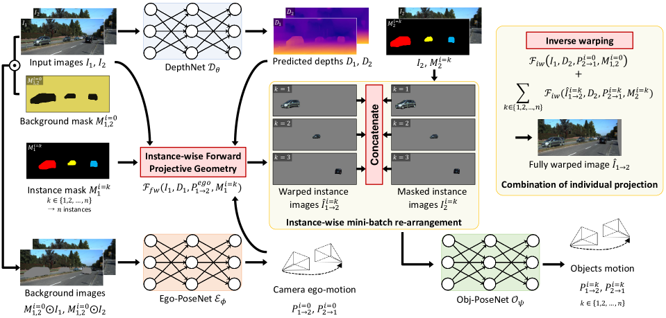
Figure 2: Overview of the proposed frameworks.

Learning motion of moving objects Recently, the joint optimization of dynamic object motion along with depth and ego-motion has gained interest as a new research topic. Cao et al. (Cao et al. 2019) propose a self-supervised framework with a given 2D bounding box to learn scene structure and 3D object motion from stereo videos. The disparity from the paired images, which is deterministic, enables computing the 3D motion vector of each instance using simple mean filtering. Gordon et al. (Gordon et al. 2019) and Li et al. (Li et al. 2020) propose a motion field network to estimate a pixel-wise transformation. It receives two consecutive rough images, which are, however, ambiguous and unclear inputs to explicitly disentangle the motion of the camera and non-rigid objects. Hence, we suggest to design the network to determine the object motion by looking at the residual signal between two images caused by pure object motion. Casser et al. (Casser et al. 2019a, b) and Klingner et al. (Klingner et al. 2020) present an unsupervised image-to-depth framework that models the motion of moving objects and cameras with given segmentation knowledge.

All the aforementioned studies use the inverse warping technique when rendering dynamic objects, which causes appearance distortion, illustrated in Fig. 1. Thus, we propose a geometrically correct projection method in dynamic situations, which is a fundamental problem in 3D geometry.

Methodology

We introduce an end-to-end joint training framework for instance-wise depth and motion learning from monocular videos without supervision as illustrated in Fig. 2. Our main contribution lies in applying the inverse and forward warping in appropriate projection situations. In this section, we introduce the instance-wise forward projective geometry and the networks for each type of output: DepthNet, Ego-PoseNet, and Obj-PoseNet. Further, we describe our novel loss functions and how they are designed for back-propagation in decomposing the background and moving object regions.

Method Overview

Baseline  Given two consecutive RGB images $(I_{1},I_{2})\in\mathbb{R}^{H\times W\times 3}$, sampled from an unlabeled video, we first predict their respective depth maps $(D_{1},D_{2})$ via our presented DepthNet $\mathcal{D}_{\theta}:\mathbb{R}^{H\times W\times 3}\rightarrow\mathbb{R}^{H\times W}$ with trainable parameters $\theta$. By concatenating two sequential images as an input, our proposed Ego-PoseNet $\mathcal{E}_{\phi}:\mathbb{R}^{2\times H\times W\times 3}\rightarrow\mathbb{R}^{6}$, with trainable parameters $\phi$, estimates the six-dimensional SE(3) relative transformation vectors $(P_{1\rightarrow 2},P_{2\rightarrow 1})$. With the predicted depth, relative ego-motion, and a given camera intrinsic matrix $K\in\mathbb{R}^{3\times 3}$, we can synthesize an adjacent image in the sequence using an inverse warping operation $\mathcal{F}_{iw}(I_{i},D_{j},P_{j\rightarrow i},K)\rightarrow\hat{I}_{i\rightarrow j}$, where $\hat{I}_{i\rightarrow j}$ is the reconstructed image by warping the reference frame $I_{i}$ (Zhou et al. 2017; Jaderberg et al. 2015). As a supervisory signal, an image reconstruction loss, $\mathcal{L}_{rec}=||I_{j}-\hat{I}_{i\rightarrow j}||_{1}$, is imposed to optimize the parameters, $\theta$ and $\phi$.

Instance-wise learning  The baseline method has a limitation that it cannot handle dynamic scenes containing moving objects. Our goal is to learn depth and ego-motion, as well as object motions, using monocular videos by constraining them with instance-wise geometric consistencies. We propose an Obj-PoseNet $\mathcal{O}_{\psi}:\mathbb{R}^{2\times H\times W\times 3}\rightarrow\mathbb{R}^{6}$ with trainable parameters $\psi$, which is specialized to estimate individual object motions. We annotate a novel video instance segmentation dataset to utilize it as an individual object mask while training the ego-motion and object motions. Given two consecutive binary instance masks $(M^{i}_{1},M^{i}_{2})\in\{0,1\}^{H\times W\times n}$ corresponding to $(I_{1},I_{2})$, $n$ instances are annotated and matched between the frames. First, in the case of camera motion, potentially moving objects are masked out and only the background region is fed to Ego-PoseNet. Secondly, the $n$ binary instance masks are multiplied to the input images and fed to Obj-PoseNet. For both networks, motions of the $k^{th}$ element are represented as $P^{i=k}_{1\rightarrow 2}$, where $k=0$ indicates camera motion from frame $I_{1}$ to $I_{2}$. The details of the motion models will be described in the following subsections.

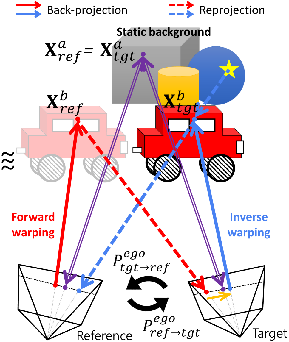
(a)

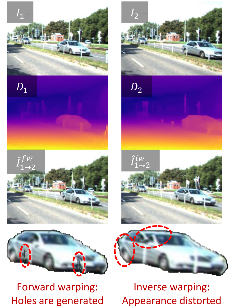
(b)

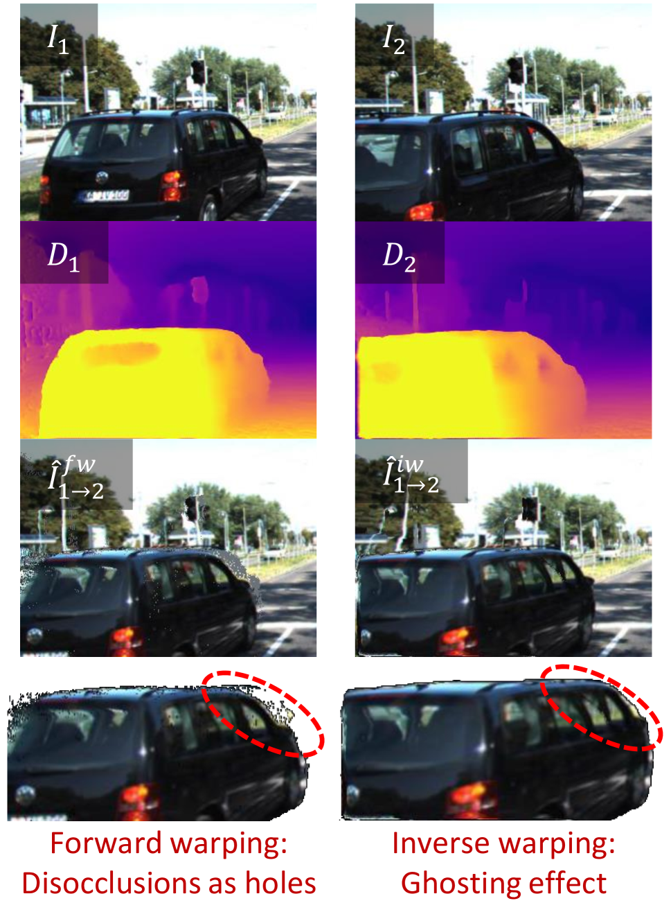
(c)

Figure 3: (a) Warping discrepancy occurs for inverse projection of moving objects. Different warping results on (b) moving and (c) close objects. $\hat{I}^{iw}$ and $\hat{I}^{fw}$ are warped only by the camera motion.

Training objectives  The previous works (Mahjourian, Wicke, and Angelova 2018; Bian et al. 2019; Chen, Schmid, and Sminchisescu 2019; Zhang et al. 2020) imposed geometric constraints between frames, but they are limited to rigid projections. Regions containing moving objects cannot be constrained with this term and are treated as outlier regions with regard to geometric consistency. In this paper, we propose instance-wise geometric consistency. We leverage instance masks to impose geometric consistency region-by-region. Following instance-wise learning, our overall objective function can be defined as follows:

where $({\mathcal{L}}_{p},{\mathcal{L}}_{g})$ are the photometric and geometric consistency losses applied on each instance region including the background, ${\mathcal{L}}_{s}$ stands for the depth smoothness loss, and $({\mathcal{L}}_{t},{\mathcal{L}}_{h})$ are the object translation and height constraint losses. $\{\lambda_{p},\lambda_{g},\lambda_{s},\lambda_{t},\lambda_{h}\}$ is the set of loss weights. We train the models in both forward ($I_{1}\rightarrow I_{2}$) and backward ($I_{2}\rightarrow I_{1}$) directions to maximally use the self-supervisory signals. In the following subsections, we introduce how to constrain the instance-wise consistencies.

Forward Projective Geometry

A fully differentiable warping function enables learning of structure-from-motion tasks. This operation is first proposed by spatial transformer networks (STN) (Jaderberg et al. 2015). Previous works for learning depth and ego-motion from unlabeled videos so far follow this grid sampling module to synthesize adjacent views. To synthesize $\hat{I}_{1\rightarrow 2}$ from $I_{1}$, the homogeneous coordinates, $p_{2}$, of a pixel in $I_{2}$ are projected to $p_{1}$ as follows:

As expressed in the equation, this operation computes $\hat{I}_{1\rightarrow 2}$ by taking the value of the homogeneous coordinates $p_{1}$ from the inverse rigid projection using $P^{i=0}_{2\rightarrow 1}$ and $D_{2}(p_{2})$. As a result, the coordinates $p_{1}$ are not valid if $p_{2}$ lies on an object that moves between $I_{1}$ and $I_{2}$. Therefore, the inverse warping is not suitable for removing the effects of ego-motion in dynamic scenes. As shown in Fig. 3(a), the inverse warping causes pixel discrepancy on a moving object, since it reprojects the point ($X^{b}_{tgt}$) from the target geometry where the 3D point has moved. This causes distortion of the appearance of moving objects as in Fig. 3(b) and ghosting effects (Janai et al. 2018) on objects near to the camera as in Fig. 3(c). To solve this problem, we define an intermediate frame which is transformed by camera motion with reference geometry, and mitigate the residual displacement (orange arrow in Fig. 3(a)) by training Obj-PoseNet as a supervisory signal. In Table 1, we describe the difference between input resources of inverse and forward warping, as well as their advantages and disadvantages.

Table 1: Comparison between inverse and forward warping.

	Inverse warping	Forward warping
Inputs	$I_{ref}$, $D_{tgt}$, $P^{ego}_{tgt\rightarrow ref}$	$I_{ref}$, $D_{ref}$, $P^{ego}_{ref\rightarrow tgt}$
Pros.	Dense registration by grid sampling.	Geometry corresponds to reference.
Cons.	Errors induced on moving objects.	Holes are generated.

In order to synthesize the novel view (from $I_{1}$ to $\hat{I}_{1\rightarrow 2}$) properly when there exist moving objects, we propose forward projective geometry, $\mathcal{F}_{fw}(I_{i},D_{i},P_{i\rightarrow j},K)\rightarrow\hat{I}_{i\rightarrow j}$ as follows:

Unlike inverse projection in Eq. (2), this warping process cannot be sampled by the STN since the projection is in the forward direction (inverse of grid sampling). In order to make this operation differentiable, we first use sparse tensor coding to index the homogeneous coordinates $p_{2}$ of a pixel in $I_{2}$. Invalid coordinates (exiting the view where $p_{2}\notin\{(x,y)|0\leq x<W,0\leq y<H\}$) of the sparse tensor are masked out. We then convert this sparse tensor to be dense by taking the nearest neighbor value of the source pixel. However, this process has a limitation that there exist irregular holes due to the sparse tensor coding. Since we need to feed those forward projected images into the neural networks in the next step, the size of the holes should be minimized. To fill these holes as much as possible, we pre-upsample the depth map $D^{\uparrow}_{1}(p_{1})$ of the reference frame. If the depth map is upsampled by a factor of $\alpha$, the camera intrinsic matrix is also upsampled as follows:

where $(f_{x},f_{y})$ are the focal lengths along the $x$- and $y$-axis. In the following subsection, we describe the steps of how to synthesize novel views with inverse and forward projection in each instance region.

Instance-Aware View Synthesis and Projection Consistency

Instance-wise projection  Each step of the instance-wise view synthesis is depicted in Fig. 2. To synthesize a novel view in an instance-wise manner, we first decompose the image region into background and object (potentially moving) regions. With given instance masks $(M^{i}_{1},M^{i}_{2})$, the background mask along frames $(I_{1},I_{2})$ is generated as

The background mask is pixel-wise multiplied ($\odot$) to the input frames $(I_{1},I_{2})$, and then concatenated along the channel axis, which is an input to Ego-PoseNet. The camera motion is computed as

To learn the object motions, we first apply the forward warping, ${\mathcal{F}}_{fw}(\cdot)$, to generate ego-motion-eliminated warped images and masks as follows:

Now we can generate forward-projected instance images as $\hat{I}^{fw,i=k}_{1\rightarrow 2}=\hat{M}^{fw,i=k}_{1\rightarrow 2}\odot\hat{I}^{fw}_{1\rightarrow 2}$ and $\hat{I}^{fw,i=k}_{2\rightarrow 1}=\hat{M}^{fw,i=k}_{2\rightarrow 1}\odot\hat{I}^{fw}_{2\rightarrow 1}$. For every object instance in the image, Obj-PoseNet predicts the $k^{th}$ object motion as

where both object motions are composed of six-dimensional SE(3) translation and rotation vectors. We merge all instance regions to synthesize the novel view. In this step, we utilize inverse warping, ${\mathcal{F}}_{iw}(\cdot)$. First, the background region is reconstructed as

where the gradients are propagated with respect to $\theta$ and $\phi$. Second, the inverse-warped $k^{th}$ instance is represented as

where the gradients are propagated with respect to $\theta$ and $\psi$. Finally, our instance-wise fully reconstructed novel view is formulated as

Instance mask propagation  Through the process of forward and inverse warping, the instance mask is also propagated to represent information on instance position and pixel validity. In the case of the $k^{th}$ instance mask $M^{i=k}_{1}$, the forward and inverse warped mask is expressed as follows:

Note that the forward warped mask $\hat{M}^{fw,i=k}_{1\rightarrow 2}$ has holes due to the sparse tensor coding. To keep the binary format and avoid interpolation near the holes while inverse warping, we round up the fractional values after each warping operation. The final valid instance mask is expressed as follows:

Instance-wise geometric consistency  We impose the geometric consistency loss for each region of an instance. With the predicted depth map and warped instance mask, $D_{1}$ can be spatially aligned to the frame $D_{2}$ by forward and inverse warping, represented as $M^{i=0}_{1,2}\odot\hat{D}^{iw,i=0}_{1\rightarrow 2}$ and $\hat{M}^{fw\rightarrow iw,i=k}_{1\rightarrow 2}\odot\hat{D}^{fw\rightarrow iw,i=k}_{1\rightarrow 2}$ respectively for background and instance regions. In addition, $D_{2}$ can be scale-consistently transformed to the frame $D_{1}$, represented as $M^{i=0}_{1,2}\odot D^{sc,i=0}_{2\rightarrow 1}$ and $\hat{M}^{fw\rightarrow iw,i=k}_{1\rightarrow 2}\odot D^{sc,i=k}_{2\rightarrow 1}$ respectively for background and instance regions. Based on this instance-wise operation, we compute the unified depth inconsistency map as:

Note that the above depth inconsistency maps are spatially aligned to the frame $D_{2}$. Therefore, we can integrate the depth inconsistency maps from the background and instance regions as follows:

Training loss  In order to handle occluded, view-exiting, and invalid instance regions, we leverage Eq. (13) and Eq. (15). We generate a weight mask as $1-D^{diff}_{1\rightarrow 2}$ and this is multiplied to the valid instance mask $\hat{M}_{1\rightarrow 2}$. Finally, our weighted valid mask is formulated as:

The photometric consistency loss ${\mathcal{L}}_{p}$ is expressed as follows:

where $\rm{x}$ is the location of each pixel, $SSIM(\cdot)$ is the structural similarity index (Wang et al. 2004), and $\gamma$ is set to 0.85 based on cross-validation. The geometric consistency loss ${\mathcal{L}}_{g}$ is expressed as follows:

To mitigate spatial fluctuation, we incorporate a smoothness term to regularize the predicted depth. We apply the edge-aware smoothness loss proposed by Ranjan et al. (Ranjan et al. 2019), which is described as:

Note that the above equations are imposed for both forward and backward directions by switching the subscripts ₁ and ₂.

Since the dataset has a low proportion of moving objects, the learned motions of objects tend to converge to zero. The same issue has been raised in a previous study (Casser et al. 2019a). To supervise the approximate amount of an object’s movement, we constrain the motion of the object with a translation prior. We compute this translation prior, $\vv{t_{p}}$, by subtracting the mean estimate of the object’s 3D points in the forward warped frame into that of the target frame’s 3D object points. This represents the mean estimated 3D vector of the object’s motion. The object translation constraint loss measures scale and cosine similarity of 3D vectors as follows:

where $\vv{t^{i=k}}$ and $\vv{t^{i=k}_{p}}$ are predicted object translation from Obj-PoseNet and the translation prior on the $k^{th}$ instance mask, and $loss_{\measuredangle}$ is a cosine similarity loss between 3D vectors.

Although we have accounted for instance-wise geometric consistency, there still exists a trivial case of infinite depth for a moving object that has the same motion as the camera motion, such as for a vehicle in front. To mitigate this issue, we adopt the object height constraint loss proposed by a previous study (Casser et al. 2019a), which is described as:

where $\overline{D}$ is the mean estimated depth, and ($p_{h}$, $h^{i=k}$) are a learnable height prior and pixel height of the $k^{th}$ instance. Unlike the previous study, for stable training, the learning rate of $p_{h}$ is reduced to $0.1$ times and the gradient of $\overline{D}$ is detached. The final loss is a weighted summation of the five loss terms, defined as Eq. (1).

Experiments

Implementation Details

Network details  For DepthNet, we use DispResNet (Ranjan et al. 2019) and a ResNet18-based encoder-decoder structure. The network can generate multi-scale outputs (six different scales), but the single-scale training converges faster and produces better performance as shown from SC-SfM (Bian et al. 2019). The structures of Ego-PoseNet and Obj-PoseNet are the same, but the weights are not shared. They consist of seven convolutional layers and regress the relative pose as three Euler angles and three translation vectors.

Training  Our system is implemented in PyTorch (Paszke et al. 2019). We train our networks using the ADAM optimizer (Kingma and Ba 2015) with $\beta_{1}=0.9$ and $\beta_{2}=0.999$ on $4\times$Nvidia RTX 2080 GPUs. The image resolution is set to $832\times 256$ and the video data is augmented with random scaling, cropping, and horizontal flipping. We set the mini-batch size to 4 and train the networks over 200 epochs with 1,000 randomly sampled batches in each epoch considering the representation capacity (Zhang et al. 2019, 2021). The initial learning rate is set to $10^{-4}$ and is decreased by half every 50 epochs. The loss weights are set to $\lambda_{p}=2.0$, $\lambda_{g}=1.0$, $\lambda_{s}=0.1$, $\lambda_{t}=0.1$, and $\lambda_{h}=0.02$.

Video instance segmentation dataset  We introduce an auto-annotation scheme to generate two video instance segmentation datasets, KITTI-VIS and Cityscapes-VIS, from existing driving datasets, KITTI (Geiger, Lenz, and Urtasun 2012) and Cityscapes (Cordts et al. 2016). To this end, we adopt an off-the-shelf instance segmentation model, e.g., Mask R-CNN (He et al. 2017) and PANet (Liu et al. 2018), and an optical flow model, PWC-Net (Sun et al. 2018), for mask propagation. We first compute the instance segmentation for every image frame, and calculate the Intersection over Union (IoU) scores among instances in each frame. If the maximal IoU in the adjacent frame is above a threshold ($\tau=0.5$), then the instance is assumed to be tracked and both masks are assigned with the same ID. The occluded regions by the bidirectional consistency check (Meister, Hur, and Roth 2018) are excluded while computing the IoU scores. The instance ID is ordered by the size of the reference instance, with the maximum size among the matched instances coming first. This size ordering is necessary, since we set the maximum number of instances with larger instances having a higher priority in the optimization. In our training, we set the maximum number of instances as three.

Table 2: Ablation study (backbone - DispResNet) on KITTI Eigen split for both background (bg.) and object (obj.) areas.

  Instance knowledge Geometric consistency Object warping AbsRel inverse forward all bg. obj.   ✗ ✗ ✗ ✗ 0.156 0.142 0.396 ✗ ✓ ✗ ✗ 0.137 0.124 0.309 ✓ ✗ ✓ ✗ 0.151 0.138 0.377 ✓ ✓ ✓ ✗ 0.146 0.131 0.362 ✓ ✗ ✗ ✓ 0.143 0.133 0.285 ✓ ✓ ✗ ✓ 0.124 0.119 0.178  

Table 3: Evaluation on KITTI 2015 scene flow training set. We evaluate the disparity compared to recent monocular-based training methods.

  Method Backbone D1 D2 bg. fg. all bg. fg. all   CC (Ranjan et al. 2019) DispResNet 35.0 42.7 36.2 – – – SC-SfM (Bian et al. 2019) DispResNet 36.0 46.5 37.5 – – – EPC++ (mono) (Luo et al. 2019) DispNet 30.7 34.4 32.7 18.4 84.6 65.6 Ours DispResNet 26.8 30.4 27.4 28.9 32.3 29.4  

Table 4: Monocular depth estimation results on the KITTI (K) Eigen test split and Cityscapes (C) test set. Models pretrained on Cityscapes and fine-tuned on KITTI are denoted by ‘C+K’. Models trained with semantic knowledge are denoted by ‘S’. For each partition, best results are written in boldface.

  Method Backbone Training Test Error metric $\downarrow$ Accuracy metric $\uparrow$ AbsRel SqRel RMSE RMSE log $\delta<1.25$ $\delta<1.25^{2}$ $\delta<1.25^{3}$   EPC++ (Luo et al. 2019) DispNet K K 0.141 1.029 5.350 0.216 0.816 0.941 0.976 CC (Ranjan et al. 2019) DispResNet K K 0.140 1.070 5.326 0.217 0.826 0.941 0.975 SC-SfM (Bian et al. 2019) DispResNet K K 0.137 1.089 5.439 0.217 0.830 0.942 0.975 Ours DispResNet K (S) K 0.124 0.886 5.061 0.206 0.844 0.948 0.979   GLNet (Chen, Schmid, and Sminchisescu 2019) ResNet18 K K 0.135 1.070 5.230 0.210 0.841 0.948 0.980 Monodepth2 (Godard et al. 2019) ResNet18 K K 0.132 1.044 5.142 0.210 0.845 0.948 0.977 Li et al. (Li et al. 2020) ResNet18 K K 0.130 0.950 5.138 0.209 0.843 0.948 0.978 Struct2Depth (Casser et al. 2019a) ResNet18 K (S) K 0.141 1.026 5.290 0.215 0.816 0.945 0.979 Gordon et al. (Gordon et al. 2019) ResNet18 K (S) K 0.128 0.959 5.230 0.212 0.845 0.947 0.976 SGDepth (Klingner et al. 2020) ResNet18 K (S) K 0.113 0.835 4.693 0.191 0.879 0.961 0.981 Ours ResNet18 K (S) K 0.112 0.777 4.772 0.191 0.872 0.959 0.982   CC (Ranjan et al. 2019) DispResNet C+K K 0.139 1.032 5.199 0.213 0.827 0.943 0.977 SC-SfM (Bian et al. 2019) DispResNet C+K K 0.128 1.047 5.234 0.208 0.846 0.947 0.976 Ours DispResNet C+K (S) K 0.119 0.863 4.984 0.202 0.856 0.950 0.980   Gordon et al. (Gordon et al. 2019) ResNet18 C+K (S) K 0.124 0.930 5.120 0.206 0.851 0.950 0.978 Ours ResNet18 C+K (S) K 0.109 0.740 4.547 0.184 0.883 0.962 0.983   Li et al. (Li et al. 2020) ResNet18 C C 0.119 1.290 6.980 0.190 0.846 0.952 0.982 Struct2Depth (Casser et al. 2019b) ResNet18 C (S) C 0.145 1.737 7.280 0.205 0.813 0.942 0.978 Gordon et al. (Gordon et al. 2019) ResNet18 C (S) C 0.127 1.330 6.960 0.195 0.830 0.947 0.981 Ours ResNet18 C (S) C 0.111 1.158 6.437 0.182 0.868 0.961 0.983  

Ablation Study

We conduct an ablation study to validate the effect of our forward projective geometry and instance-wise geometric consistency term on monocular depth estimation. The ablation is performed with the KITTI Eigen split (Eigen, Puhrsch, and Fergus 2014). The models are validated with the AbsRel metric by separating the background and object areas, which are masked by our annotation. As described in Table 2, we first evaluate SC-SfM (Bian et al. 2019) as a baseline, which is not trained with instance knowledge (the $1^{st}$ and $2^{nd}$ models). Since there are no instance masks, DepthNet is trained by inverse warping the whole image. The results show that the geometric consistency term over the whole image plane boosts the performance of depth estimation. With the given instance masks, we try both inverse and forward warping on the object areas. The inverse warping on the objects slightly improves the depth estimation; however, we observe that Obj-PoseNet does not converge (the $3^{rd}$ and $4^{th}$ models). Rather, the performance is degraded when using the instance-wise geometric consistency term with inverse warping on the objects (comparing the $2^{nd}$ and $4^{th}$ models). We conjecture that the uncertainty in learning the depth of the object area degrades the performance on the background depth around which the object is moving. However, the forward warping on the objects improves the depth estimation on both background and object areas (the $5^{th}$ and $6^{th}$ models). This shows that a well-optimized Obj-PoseNet helps to boost the performance of DepthNet and they complement each other. We note that the background is still inverse warped to synthesize the target view and the significant performance improvement comes from the instance-wise geometric loss incorporated with forward projection while warping the object areas.

Table 5: Absolute trajectory error (ATE) on KITTI visual odometry.

  Method Seq. 09 Seq. 10   SfM-Learner (Zhou et al. 2017) $0.021\pm 0.017$ $0.020\pm 0.015$ GeoNet (Yin and Shi 2018) $0.012\pm 0.007$ $0.012\pm 0.009$ CC (Ranjan et al. 2019) $0.012\pm 0.007$ $0.012\pm 0.008$ Struct2Depth (Casser et al. 2019a) $0.011\pm 0.006$ $0.011\pm 0.010$ GLNet (Chen, Schmid, and Sminchisescu 2019) $0.011\pm 0.006$ $0.011\pm 0.009$ SGDepth (Klingner et al. 2020) $0.017\pm 0.009$ $0.014\pm 0.010$   Ours (w/o inst.) $0.012\pm 0.008$ $0.011\pm 0.010$ Ours (w/ inst.) $\mathbf{0.010\pm 0.013}$ $\mathbf{0.011\pm 0.008}$  

Table 6: Relative translation $t_{err}$ ($\%$) and rotation $r_{err}$ ($\nicefrac{{{}^{\circ}}}{{100m}}$) errors on KITTI visual odometry.

  Method Seq. 09 Seq. 10 $t_{err}$ $r_{err}$ $t_{err}$ $r_{err}$   GeoNet (Yin and Shi 2018) 39.4 14.3 29.0 8.6 SC-SfM (Bian et al. 2019) 11.2 3.4 10.1 5.0   Ours (w/o inst.) 10.2 5.2 10.1 4.8 Ours (w/ inst.) 8.6 2.9 9.2 4.5  

Monocular Depth Estimation

Test setup  First, we show the disparity results on the KITTI 2015 scene flow training set. Our models are trained with non-overlapped KITTI raw images. We follow the standard metrics (D1, D2: percentage of erroneous pixels over all pixels). Since monocular training has a scale issue, we assume that the scale for disparity is given, which is the same experimental setup in EPC++ (Luo et al. 2019).

Second, we train and test our models with the Eigen split (Eigen, Puhrsch, and Fergus 2014) of the KITTI dataset, and the Cityscapes dataset following the method from Struct2Depth (Casser et al. 2019a). We compare the performance of the proposed method with recent state-of-the-art works (Chen, Schmid, and Sminchisescu 2019; Casser et al. 2019a; Bian et al. 2019; Ranjan et al. 2019; Godard et al. 2019; Gordon et al. 2019; Klingner et al. 2020; Li et al. 2020) for unsupervised single-view depth estimation.

Results analysis  Table 3 shows the results on KITTI 2015 scene flow. The foreground (fg.) results show the superiority on handling dynamic regions. Table 4 shows the KITTI Eigen split and Cityscapes test results, where ours achieves state-of-the-art performance in the single-view depth prediction task with unsupervised monocular training. The advantage is evident from using instance masks and constraining the instance-wise photometric and geometric consistencies. Note that we do not need instance masks for DepthNet in testing.

Visual Odometry

Test setup  We evaluate the performance of our Ego-PoseNet on the KITTI visual odometry dataset. Following the evaluation setup of SfM-Learner (Zhou et al. 2017), we use sequences 00-08 for training, and sequences 09 and 10 for tests. In our case, since the potentially moving object masks are fed together with the image sequences while training Ego-PoseNet, we test the performance of visual odometry under two conditions: with and without instance masks.

Results analysis  We measure the absolute trajectory error (ATE) in Table 5 and relative errors ($t_{err}$, $r_{err}$) in Table 6, which show state-of-the-art performance. Although we do not use the instance mask, the result of sequence 10 produces favorable performance. This is because the scene does not have many potentially moving objects, e.g., vehicles and pedestrians, so the result is not affected much by using or not using instance masks.

Conclusion

In this work, we propose a unified framework that predicts monocular depth, ego-motion, and 6-DoF motion of multiple dynamic objects by training on monocular videos. Leveraging video instance segmentation, we design an end-to-end joint training pipeline. There are three main contributions of our work: (1) a neural forward projection module, (2) a unified instance-aware photometric and geometric consistency loss, and (3) an auto-annotation scheme for video instance segmentation. We show that our method outperforms the existing unsupervised methods that estimate monocular depth. We also show that each proposed module plays a role in improving the performance of our framework.

Acknowledgements

This research was supported by the Shared Sensing for Cooperative Cars Project funded by Bosch (China) Investment Ltd. This work was supported by the National Research Foundation of Korea (NRF) grant funded by the Korea government (MSIT) (No. 2020R1C1C1013210), and the DGIST R&D Program of the Ministry of Science and ICT (20-CoE-IT-01).

References

- Behley et al. (2019) Behley, J.; Garbade, M.; Milioto, A.; Quenzel, J.; Behnke, S.; Stachniss, C.; and Gall, J. 2019. SemanticKITTI: A Dataset for Semantic Scene Understanding of LiDAR Sequences. In ICCV.
- Bian et al. (2019) Bian, J.-W.; Li, Z.; Wang, N.; Zhan, H.; Shen, C.; Cheng, M.-M.; and Reid, I. 2019. Unsupervised Scale-consistent Depth and Ego-motion Learning from Monocular Video. In NeurIPS.
- Cao et al. (2019) Cao, Z.; Kar, A.; Hane, C.; and Malik, J. 2019. Learning Independent Object Motion from Unlabelled Stereoscopic Videos. In CVPR.
- Casser et al. (2019a) Casser, V.; Pirk, S.; Mahjourian, R.; and Angelova, A. 2019a. Depth prediction without the sensors: Leveraging structure for unsupervised learning from monocular videos. In AAAI.
- Casser et al. (2019b) Casser, V.; Pirk, S.; Mahjourian, R.; and Angelova, A. 2019b. Unsupervised monocular depth and ego-motion learning with structure and semantics. In CVPRw.
- Chang and Chen (2018) Chang, J.-R.; and Chen, Y.-S. 2018. Pyramid stereo matching network. In CVPR.
- Chen et al. (2019) Chen, P.-Y.; Liu, A. H.; Liu, Y.-C.; and Wang, Y.-C. F. 2019. Towards scene understanding: Unsupervised monocular depth estimation with semantic-aware representation. In CVPR.
- Chen, Schmid, and Sminchisescu (2019) Chen, Y.; Schmid, C.; and Sminchisescu, C. 2019. Self-Supervised Learning With Geometric Constraints in Monocular Video: Connecting Flow, Depth, and Camera. In ICCV.
- Cordts et al. (2016) Cordts, M.; Omran, M.; Ramos, S.; Rehfeld, T.; Enzweiler, M.; Benenson, R.; Franke, U.; Roth, S.; and Schiele, B. 2016. The cityscapes dataset for semantic urban scene understanding. In CVPR.
- Dosovitskiy et al. (2015) Dosovitskiy, A.; Fischer, P.; Ilg, E.; Hausser, P.; Hazirbas, C.; Golkov, V.; Van Der Smagt, P.; Cremers, D.; and Brox, T. 2015. Flownet: Learning optical flow with convolutional networks. In ICCV.
- Eigen, Puhrsch, and Fergus (2014) Eigen, D.; Puhrsch, C.; and Fergus, R. 2014. Depth map prediction from a single image using a multi-scale deep network. In NIPS.
- Garg et al. (2016) Garg, R.; BG, V. K.; Carneiro, G.; and Reid, I. 2016. Unsupervised cnn for single view depth estimation: Geometry to the rescue. In ECCV.
- Geiger et al. (2014) Geiger, A.; Lauer, M.; Wojek, C.; Stiller, C.; and Urtasun, R. 2014. 3d traffic scene understanding from movable platforms. IEEE Transactions on Pattern Analysis and Machine Intelligence (PAMI) .
- Geiger, Lenz, and Urtasun (2012) Geiger, A.; Lenz, P.; and Urtasun, R. 2012. Are we ready for autonomous driving? the kitti vision benchmark suite. In CVPR.
- Godard, Mac Aodha, and Brostow (2017) Godard, C.; Mac Aodha, O.; and Brostow, G. J. 2017. Unsupervised monocular depth estimation with left-right consistency. In CVPR.
- Godard et al. (2019) Godard, C.; Mac Aodha, O.; Firman, M.; and Brostow, G. J. 2019. Digging into self-supervised monocular depth estimation. In ICCV.
- Gordon et al. (2019) Gordon, A.; Li, H.; Jonschkowski, R.; and Angelova, A. 2019. Depth from videos in the wild: Unsupervised monocular depth learning from unknown cameras. In ICCV.
- Guizilini et al. (2020a) Guizilini, V.; Ambrus, R.; Pillai, S.; Raventos, A.; and Gaidon, A. 2020a. 3D Packing for Self-Supervised Monocular Depth Estimation. In CVPR.
- Guizilini et al. (2020b) Guizilini, V.; Hou, R.; Li, J.; Ambrus, R.; and Gaidon, A. 2020b. Semantically-Guided Representation Learning for Self-Supervised Monocular Depth. In ICLR.
- He et al. (2017) He, K.; Gkioxari, G.; Dollár, P.; and Girshick, R. 2017. Mask r-cnn. In ICCV.
- Hur and Roth (2020) Hur, J.; and Roth, S. 2020. Self-Supervised Monocular Scene Flow Estimation. In CVPR.
- Jaderberg et al. (2015) Jaderberg, M.; Simonyan, K.; Zisserman, A.; et al. 2015. Spatial transformer networks. In NIPS.
- Janai et al. (2018) Janai, J.; Guney, F.; Ranjan, A.; Black, M.; and Geiger, A. 2018. Unsupervised learning of multi-frame optical flow with occlusions. In ECCV.
- Kingma and Ba (2015) Kingma, D. P.; and Ba, J. 2015. Adam: A method for stochastic optimization. In ICLR.
- Klingner et al. (2020) Klingner, M.; Termöhlen, J.-A.; Mikolajczyk, J.; and Fingscheidt, T. 2020. Self-Supervised Monocular Depth Estimation: Solving the Dynamic Object Problem by Semantic Guidance. In ECCV.
- Lee et al. (2015) Lee, S.; Huh, S.; Yoo, D.; Kweon, I. S.; and Shim, D. H. 2015. Rich feature hierarchies from omni-directional RGB-DI information for pedestrian detection. In URAI.
- Lee et al. (2019a) Lee, S.; Im, S.; Lin, S.; and Kweon, I. S. 2019a. Learning Residual Flow as Dynamic Motion from Stereo Videos. In IROS.
- Lee et al. (2019b) Lee, S.; Kim, J.; Oh, T.-H.; Jeong, Y.; Yoo, D.; Lin, S.; and Kweon, I. S. 2019b. Visuomotor Understanding for Representation Learning of Driving Scenes. In BMVC.
- Lee et al. (2017) Lee, S.; Kim, J.; Shin Yoon, J.; Shin, S.; Bailo, O.; Kim, N.; Lee, T.-H.; Seok Hong, H.; Han, S.-H.; and So Kweon, I. 2017. VPGNet: Vanishing Point Guided Network for Lane and Road Marking Detection and Recognition. In ICCV.
- Li et al. (2020) Li, H.; Gordon, A.; Zhao, H.; Casser, V.; and Angelova, A. 2020. Unsupervised monocular depth learning in dynamic scenes. In CoRL.
- Liu et al. (2020) Liu, P.; King, I.; Lyu, M. R.; and Xu, J. 2020. Flow2Stereo: Effective Self-Supervised Learning of Optical Flow and Stereo Matching. In CVPR.
- Liu et al. (2019) Liu, P.; Lyu, M.; King, I.; and Xu, J. 2019. Selflow: Self-supervised learning of optical flow. In CVPR.
- Liu et al. (2018) Liu, S.; Qi, L.; Qin, H.; Shi, J.; and Jia, J. 2018. Path aggregation network for instance segmentation. In CVPR.
- Luo et al. (2019) Luo, C.; Yang, Z.; Wang, P.; Wang, Y.; Xu, W.; Nevatia, R.; and Yuille, A. 2019. Every Pixel Counts++: Joint Learning of Geometry and Motion with 3D Holistic Understanding. IEEE Transactions on Pattern Analysis and Machine Intelligence (PAMI) .
- Lv et al. (2018) Lv, Z.; Kim, K.; Troccoli, A.; Sun, D.; Rehg, J. M.; and Kautz, J. 2018. Learning rigidity in dynamic scenes with a moving camera for 3d motion field estimation. In ECCV.
- Mahjourian, Wicke, and Angelova (2018) Mahjourian, R.; Wicke, M.; and Angelova, A. 2018. Unsupervised Learning of Depth and Ego-Motion from Monocular Video Using 3D Geometric Constraints. In CVPR.
- Mayer et al. (2016) Mayer, N.; Ilg, E.; Hausser, P.; Fischer, P.; Cremers, D.; Dosovitskiy, A.; and Brox, T. 2016. A large dataset to train convolutional networks for disparity, optical flow, and scene flow estimation. In CVPR.
- Meister, Hur, and Roth (2018) Meister, S.; Hur, J.; and Roth, S. 2018. UnFlow: Unsupervised Learning of Optical Flow with a Bidirectional Census Loss. In AAAI.
- Paszke et al. (2019) Paszke, A.; Gross, S.; Massa, F.; Lerer, A.; Bradbury, J.; Chanan, G.; Killeen, T.; Lin, Z.; Gimelshein, N.; Antiga, L.; et al. 2019. Pytorch: An imperative style, high-performance deep learning library. In NeurIPS.
- Pillai, Ambruş, and Gaidon (2019) Pillai, S.; Ambruş, R.; and Gaidon, A. 2019. Superdepth: Self-supervised, super-resolved monocular depth estimation. In ICRA.
- Ranjan et al. (2019) Ranjan, A.; Jampani, V.; Kim, K.; Sun, D.; Wulff, J.; and Black, M. J. 2019. Competitive Collaboration: Joint Unsupervised Learning of Depth, Camera Motion, Optical Flow and Motion Segmentation. In CVPR.
- Shashua, Gdalyahu, and Hayun (2004) Shashua, A.; Gdalyahu, Y.; and Hayun, G. 2004. Pedestrian detection for driving assistance systems: Single-frame classification and system level performance. In IEEE Intelligent Vehicles Symposium.
- Shin, Kwon, and Tomizuka (2019) Shin, K.; Kwon, Y. P.; and Tomizuka, M. 2019. Roarnet: A robust 3d object detection based on region approximation refinement. In 2019 IEEE Intelligent Vehicles Symposium (IV).
- Sun et al. (2018) Sun, D.; Yang, X.; Liu, M.-Y.; and Kautz, J. 2018. Pwc-net: Cnns for optical flow using pyramid, warping, and cost volume. In CVPR.
- Wang et al. (2018a) Wang, C.; Buenaposada, J. M.; Zhu, R.; and Lucey, S. 2018a. Learning Depth from Monocular Videos using Direct Methods. In CVPR.
- Wang et al. (2019) Wang, Y.; Wang, P.; Yang, Z.; Luo, C.; Yang, Y.; and Xu, W. 2019. Unos: Unified unsupervised optical-flow and stereo-depth estimation by watching videos. In CVPR.
- Wang et al. (2018b) Wang, Y.; Yang, Y.; Yang, Z.; Zhao, L.; Wang, P.; and Xu, W. 2018b. Occlusion aware unsupervised learning of optical flow. In CVPR.
- Wang et al. (2004) Wang, Z.; Bovik, A. C.; Sheikh, H. R.; and Simoncelli, E. P. 2004. Image quality assessment: from error visibility to structural similarity. IEEE Transactions on Image Processing .
- Yang, Fan, and Xu (2019) Yang, L.; Fan, Y.; and Xu, N. 2019. Video Instance Segmentation. In ICCV.
- Yang et al. (2018) Yang, Z.; Wang, P.; Wang, Y.; Xu, W.; and Nevatia, R. 2018. Lego: Learning edge with geometry all at once by watching videos. In CVPR.
- Yin and Shi (2018) Yin, Z.; and Shi, J. 2018. Geonet: Unsupervised learning of dense depth, optical flow and camera pose. In CVPR.
- Zhang et al. (2021) Zhang, C.; Benz, P.; Argaw, D. M.; Lee, S.; Kim, J.; Rameau, F.; Bazin, J.-C.; and Kweon, I. S. 2021. Resnet or densenet? introducing dense shortcuts to resnet. In WACV.
- Zhang et al. (2020) Zhang, C.; Rameau, F.; Kim, J.; Argaw, D. M.; Bazin, J.-C.; and Kweon, I. S. 2020. DeepPTZ: Deep Self-Calibration for PTZ Cameras. In WACV.
- Zhang et al. (2019) Zhang, C.; Rameau, F.; Lee, S.; Kim, J.; Benz, P.; Argaw, D. M.; Bazin, J.-C.; and Kweon, I. S. 2019. Revisiting Residual Networks with Nonlinear Shortcuts. In BMVC.
- Zhou et al. (2017) Zhou, T.; Brown, M.; Snavely, N.; and Lowe, D. G. 2017. Unsupervised learning of depth and ego-motion from video. In CVPR.