Nonlinear diffusion in transparent media

Abstract

We consider a prototypical nonlinear parabolic equation whose flux has three distinguished features: it is nonlinear with respect to both the unknown and its gradient, it is homogeneous, and it depends only on the direction of the gradient. For such equation, we obtain existence and uniqueness of entropy solutions to the Dirichlet problem, the homogeneous Neumann problem, and the Cauchy problem. Qualitative properties of solutions, such as finite speed of propagation and the occurrence of waiting-time phenomena, with sharp bounds, are shown. We also discuss the formation of jump discontinuities both at the boundary of the solutions’ support and in the bulk.

Keywords: Parabolic Equations, Dirichlet problem, Cauchy problem, Neumann problem, Entropy solutions, Flux-saturated diffusion equations, Waiting time phenomena, Conservation laws

MSC Classification [2020] 35K20, 35D99, 35K67, 35L65

1 Introduction

The paper is concerned with the following PDE:

$$u_{t}=\operatorname{div}\left(u^{m}\frac{\nabla u}{|\nabla u|}\right){.}$$ (1)

Two particular values of the parameter $m$ lead to well known equations. When $m=0$, (1) coincides with the total variation flow: we refer to the monograph [4] for a detailed study of the subject and to [31] for its applications in image processing. The case $m=1$ (the so-called heat equation in transparent media) was considered in [8], where existence and uniqueness of entropy solutions to the Cauchy problem for (1) were obtained. In addition, the authors showed that solutions to the relativistic heat equation,

$$\frac{\partial u}{\partial t}=\varrho\operatorname{div}\left(u\frac{\nabla u}{\sqrt{u^{2}+\varrho^{2}|\nabla u|^{2}}}\right),$$ (2)

converge to solutions of (1) (with $m=1$) as $\varrho\to+\infty$.

Our focus is on the case $m>1$, in which (1) is the formal limit of the relativistic porous medium equation,

$$\frac{\partial u}{\partial t}=\varrho\operatorname{div}\left(\frac{{u^{m}}\nabla u}{\sqrt{u^{2}+\varrho^{2}|\nabla u|^{2}}}\right),\quad m>1\,,$$ (3)

as the kinematic viscosity $\varrho$ tends to $+\infty$ (here the maximal speed of propagation has been normalized to $1$). Eq. (3) was introduced in [29, 30] while studying heat diffusion in neutral gases (precisely with $m=3/2$). Existence and uniqueness of solutions to the Cauchy problem associated to (3) were obtained in [6]. This equation has received recently some attention and different key-features of solutions, such as propagation of support, waiting time phenomena, speed of discontinuity fronts, and pattern formations, have been addressed by many authors [7, 21, 25, 26, 17, 18, 19].

Our interest in Eq. (1) is twofold.

Shock formation.. First of all, the dynamics of shock formation for solutions to (3) is not yet fully understood in this type of parabolic equations with hyperbolic phenomena. The studies are limited to some equations related to (3) in the pioneering contributions [14, 16, 15] and to numerical simulations [11, 20]. Since (1) and (3) formally coincide where $|\nabla u|\gg 1$, in particular at discontinuity fronts, (1) could serve as a prototype equation for investigating such phenomena. Moreover, Eq. (1) has two scaling invariances: thus one can expect to clarify and study qualitatively the strong interplays between hyperbolic and parabolic mechanisms in this type of flux–limited diffusion equations.

Well-posedness. (1) stands as a model for autonomous evolution equations in divergence form which, though of second order, have the same scaling as that of a first order nonlinear conservation law. For this type of equations, a well-posedness theory is not known at our best knowledge.

Concerning well-posedness, we will consider the Dirichlet problem, the homogeneous Neumann problem (both in a bounded domain $\Omega$), and the Cauchy problem. Our arguments rely on nonlinear semigroup theory. In a bounded domain $\Omega$, in [27] we studied the resolvent equation of (1), i.e.

$$u-f=\operatorname{div}\left(u^{m}\frac{\nabla u}{|\nabla u|}\right)\quad\mbox{in }\ \Omega,$$ (4)

and we obtained existence and contraction in $L^{1}(\Omega)$ (see Theorem 3.5 below). By associating an $m-$accretive operator in $L^{1}(\Omega)$ to solutions to (4) we obtain existence of a mild solution to (1). In order to characterize such solution, we introduce a definition of entropy solutions and subsolutions to (1) and we prove that the semigroup solution is in fact an entropy solution. Finally, we show that a comparison principle holds in $L^{1}$ between subsolutions and solutions, which yields uniqueness of solutions. This programme is worked out in Section 3 for the nonhomogeneous Dirichlet problem associated to (1), while the corresponding results for the homogeneous Neumann problem and the Cauchy problem are discussed in Section 4 and 6, respectively.

The second main objective of this paper is to study qualitative properties of solutions to (1). In Section 5, we construct a family of compactly supported self-similar ${S}BV$-solutions: together with the comparison principle, this permits to show the finite speed of propagation property. In Section 6, thanks to the finite speed of propagation property, we obtain existence and uniqueness of solutions to the Cauchy problem for bounded and compactly supported initial data. There, we also characterize entropy solutions as those distributional solutions that satisfy the corresponding Rankine-Hugoniot jump conditions (together with an inequality for the Cantor part, if any). In Section 7 we perform a complete study of the waiting time phenomenon: we show that there is a scaling-wise sharp bound on the behavior at the boundary of the solutions’ support, which discriminates between occurrence and non-occurrence of a waiting time phenomenon. The corresponding results for Eq. (3) are contained in [25, 26]. Finally, in the one-dimensional case we discuss similarities and differences between the behavior of solutions to (1) and those of the Burger’s equation. This is done in Section 8, where we also show that the formation of jump discontinuities may take place both at the boundary of the solution’s support and in the bulk.

2 Preliminaries and Notation

Throughout the paper, $m>1$ and $\Omega$ is a bounded open subset of ${\mathbb{R}}^{N}$ with Lipschitz boundary $\partial\Omega$. For a general $\ell\in L^{1}_{loc}(\mathbb{R})$, we let

$$J_{\ell}(s)=\int_{0}^{s}\ell(\sigma)\ d\sigma\,,\ \ \text{and}\ \ \ \Phi_{\ell}(s)=\int_{0}^{s}\ell^{\prime}(\sigma)\varphi(\sigma)\ d\sigma\,,$$ (5)

where we have written $\varphi(s):=s^{m}$, for $s>0$ to ease the notation. Moreover, let

$$\mathcal{L}=\{\ell:[0,\infty)\to[0,\infty):\ \ell^{\prime}\geq 0,\ {\rm Lip}(\ell)<\infty,\ {\ell(0)=0,}\ {\rm supp}({\ell^{\prime}})\subset(0,\infty{)}\}\,.$$

For $a,b,l\in[-\infty,+\infty]$ we let

$$T_{a,b}^{l}(r)=\max\{\min\{b,r\},a\}-l,$$

and we define, for $r\geq 0$,

$$\mathcal{T}_{+}=\{T_{a,b}^{l}:\ 0<a<b,\ l\leq a\}.$$

For a given $T=T_{a,b}^{l}\in\mathcal{T}_{+}$, we let $T^{0}:=T+l=T_{a,b}^{0}.$ The subscript $+$ on a function space denotes that the functions within it are nonnegative.

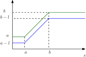
Figure 1: $\color[rgb]{0,0,1}T_{a,b}^{l}(s)$ and $\ {\color[rgb]{0,0.6,0}T_{a,b}^{0}(s)}$

We denote by $\mathcal{H}^{N-1}$ the $(N-1)$-dimensional Hausdorff measure, by $\mathcal{L}^{N}$ the $N$-dimensional Lebesgue measure, and by ${\mathcal{M}}(\Omega)$ the space of finite Radon measures on $\Omega$ (see [3, Def. 1.40]). The subscript ₀ denotes spaces of compactly supported functions. We recall that ${\mathcal{M}}(\Omega)$ is the dual space of $C_{0}(\Omega)$. We let $\mathcal{D}(\Omega):=C_{0}^{\infty}(\Omega)$ and $\mathcal{D}^{\prime}(\Omega)$ its dual.

When no ambiguity arises, we shall often make use of the simplified notation $\|v\|_{q}$, $1\leq q\leq\infty$ to indicate the Lebesgue norms of $v$; here $v$ can be either a scalar function in $L^{q}(\Omega)$ or a vector field in $(L^{q}(\Omega))^{N}$ (usually indicated by ${\bf v}$). From time to time we will also use the following notation:

$$\int_{\Omega}f(x)\,{\mathrm{d}}x:=\int_{\Omega}f\,.$$

2.1 The space $L^{\infty}_{loc,w}((0,\tau];\mathcal{M}(\Omega))$

For $\tau\in(0,+\infty]$ we denote by $L^{\infty}_{loc,w}((0,\tau];\mathcal{M}(\Omega))$ the set of measures $\mu\in\mathcal{M}(Q_{\tau})$ for which for a.e. $t\in(0,\tau)$ there is a measure $\mu(\cdot,t)\in\mathcal{M}(\Omega)$ such that:

• for all $\zeta\in C_{c}(Q_{\tau})$ the map $t\mapsto\left\langle\mu(\cdot,t),\zeta(\cdot,t)\right\rangle_{\Omega}$ belongs to $L^{1}(0,\tau)$ and

  $$\left\langle\mu,\zeta\right\rangle_{Q_{\tau}}=\int_{0}^{\tau}\left\langle\mu(\cdot,t),\zeta(\cdot,t)\right\rangle_{\Omega}\,dt\,;$$ (6)

• the map $t\mapsto\|\mu(t)\|_{\mathcal{M}(\Omega)}$ belongs to $L^{\infty}_{loc}((0,\tau])$.

Accordingly, for $0<\overline{\tau}<\tau$, we use the notation

$$\|\mu\|_{L^{\infty}_{w}([\overline{\tau},\tau];\mathcal{M}(\Omega))}:=\mbox{ess}\sup_{t\in(\overline{\tau},\tau)}\|\mu(t)\|_{\mathcal{M}(\Omega)}\quad\text{for $\mu\in L^{\infty}_{loc,w}((0,\tau];\mathcal{M}(\Omega))$\,.}$$

Observe that by the above definition the map $t\mapsto\left\langle\mu(\cdot,t),\rho\right\rangle_{\Omega}$ is measurable for all $\rho\in C_{c}(\Omega)$, thus the map $(0,\tau)\ni t\mapsto\mu(t)\in\mathcal{M}(\Omega)$ is weakly* measurable.

2.2 $TBV$-functions

We use standard notations and concepts for $BV$ functions as in [3]; in particular, for $u\in BV({\mathbb{R}}^{N})$, $\nabla u\mathcal{L}^{N}$, resp. $D^{s}u$, denote the absolutely continuous, resp. singular, parts of $Du$ with respect to the Lebesgue measure $\mathcal{L}^{N}$, $\tilde{\nabla}u$ denotes the diffuse part of $Du$; i.e. $\tilde{\nabla}u:=\nabla u\mathcal{L}^{N}+D^{c}u$, with $D^{c}u$ is the Cantor part of $Du$, $J_{u}$ denotes its jump set. For any $BV$-function $u$, we denote $[u]:=u^{+}-u^{-}$ on $J_{u}$. From now on, we will always identify a $BV$-function with its precise representative.

Let

$$TBV_{+}(\Omega)=\{u\in L^{1}(\Omega;[0,+\infty)):\ T_{a,\infty}^{0}(u)\in BV(\Omega)\ \mbox{for all }a>0\}.$$

Given $u\in L^{1}_{loc}(\Omega)$, the upper and lower approximate limits of $u$ at a point $x\in\Omega$ are defined respectively as

$$u^{\vee}(x) := \inf\{t\in{\mathbb{R}}:\lim_{\rho\downarrow 0}\rho^{-N}|\{u>t\}\cap B_{\rho}(x)|=0\},$$

$$u^{\wedge}(x) := \sup\{t\in{\mathbb{R}}:\lim_{\rho\downarrow 0}\rho^{-N}|\{u<t\}\cap B_{\rho}(x)|=0\}.$$

We let $S_{u}^{*}:=\{x\in\Omega:u^{\wedge}(x)<u^{\vee}(x)\}$ and

$$DTBV_{+}(\Omega)=\{u\in TBV_{+}(\Omega):\ \mathcal{H}^{N-1}(S_{u}^{*})=0\}.$$ (7)

The set of weak approximate jump points is the subset $J_{u}^{*}$ of $S_{u}^{*}$ such that there exists a unit vector $\nu_{u}^{*}(x)\in{\mathbb{R}}^{N}$ such that the weak approximate limit of the restriction of $u$ to the hyperplane $H^{+}:=\{y\in\Omega:\langle y-x,\nu_{u}^{*}(x)\rangle>0\}$ is $u^{\vee}(x)$ and the weak approximate limit of the restriction of $u$ to $H^{-}:=\{y\in\Omega:\langle y-x,\nu_{u}^{*}(x)\rangle<0\}$ is $u^{\wedge}(x)$. In [3, Page 237] it is shown that for any $u\in L^{1}_{loc}(\Omega)$, $J_{u}\subset J_{u}^{*}$. Moreover, $u^{\vee}(x)=\max\{u^{+}(x),u^{-}(x)\}$, $u^{\wedge}(x)=\min\{u^{+}(x),u^{-}(x)\}$ and $\nu_{u}^{*}(x)=\pm\nu_{u}(x)$ for any $x\in J_{u}$. Furthermore, ([27, Lemma 2.1] $S_{u}^{*}$ is countably $\mathcal{H}^{N-1}$ rectifiable and $\mathcal{H}^{N-1}(S_{u}^{*}\setminus J_{u}^{*})=0$.

Finally, $TBV_{+}(\Omega)$ functions have a well defined trace on the boundary $\partial\Omega$ (see [27, Lemma 5.1].

Given $u\in TBV_{+}(\Omega)$ we use the following notation for consistency with previous works, e.g. [5, 6, 7, 8, 9, 10, 26]:

$$h(u,D\ell(u))=|D\Phi_{\ell}(u)|\,.$$

2.3 Divergence-measure vector-fields

We define the space

$$X_{\mathcal{M}}(\Omega)=\left\{{\bf z}\in L^{\infty}(\Omega;{\mathbb{R}}^{N})\ :\,\operatorname{div}{\bf z}\in{\mathcal{M}}(\Omega)\right\}.$$

In [12, Theorem 1.2] (see also [4, 22]), the weak trace on $\partial\Omega$ of the normal component of ${\bf z}\in X_{\mathcal{M}}(\Omega)$ is defined as a linear operator $[\cdot,\nu^{\Omega}]:X_{\mathcal{M}}(\Omega)\rightarrow L^{\infty}(\partial\Omega)$ such that $\|\,[{\bf z},\nu^{\Omega}]\,\|_{L^{\infty}(\partial\Omega)}\leq\|{\bf z}\|_{\infty}$ for all ${\bf z}\in X_{\mathcal{M}}(\Omega)$ and $[{\bf z},\nu^{\Omega}]$ coincides with the point-wise trace of the normal component if ${\bf z}$ is smooth, i.e.

$$[{\bf z},\nu^{\Omega}](x)={\bf z}(x)\cdot\nu^{\Omega}(x)\quad\hbox{for all}\ x\in\partial\Omega\ \ \hbox{if}\ {\bf z}\in C^{1}(\overline{\Omega},{\mathbb{R}}^{m}).$$

It follows from [22, Proposition 3.1] or [2, Proposition 3.4] that $\operatorname{div}{\bf z}$ is absolutely continuous with respect to $\mathcal{H}^{N-1}$. Therefore, given ${\bf z}\in X_{\mathcal{M}}(\Omega)$ and $u\in BV(\Omega)\cap L^{\infty}(\Omega)$, the functional $({\bf z},Du)\in\mathcal{D}^{\prime}(\Omega)$ given by

$$\langle({\bf z},Du),\psi\rangle:=-\int_{\Omega}u\,\psi\,{\mathrm{d}}(\operatorname{div}{\bf z})-\int_{\Omega}u\,{\bf z}\nabla\psi\,{\mathrm{d}}x\,$$ (8)

is well defined, and the following holds (see [21], Lemma 5.1, Theorem 5.3, Lemma 5.4, and Lemma 5.6).

Lemma 2.1.

Let ${\bf z}\in X_{\mathcal{M}}(\Omega)$ and $u\in BV(\Omega)\cap L^{\infty}(\Omega)$. Then the functional $({\bf z},Du)\in\mathcal{D}^{\prime}(\Omega)$ defined by (8) is a Radon measure which is absolutely continuous with respect to $|Du|$. Furthermore

$$\int_{\Omega}u\,{\mathrm{d}}(\operatorname{div}{\bf z})+({\bf z},Du)(\Omega)=\int_{\partial\Omega}[{\bf z},\nu^{\Omega}]u\,{\mathrm{d}}\mathcal{H}^{m-1}$$ (9)

and

$$\operatorname{div}(u{\bf z})=u\operatorname{div}{\bf z}+({\bf z},Du)\,\quad{\rm as\ measures.}$$ (10)

3 Entropy solution to the Dirichlet problem

Let $\tau\in(0,+\infty]$. In this Section we consider the following problem:

$$\left\{\begin{array}[]{ll}u_{t}=\displaystyle\operatorname{div}\left(u^{m}\frac{\nabla u}{|\nabla u|}\right)&{\rm in\ }{Q_{\rm\tau}:=(0,{\rm\tau})\times\Omega}\\[4.30554pt] u(0,x)=u_{0}&{\rm in\ }\Omega\\ u=g&{\rm on\ }{S_{\rm\tau}:=(0,{\rm\tau})\times\partial\Omega}\end{array}\right.$$ (11)

3.1 Definition of entropy solution

A solution to problem (11) is defined as follows.

Definition 3.1.

Let $u_{0}\in L^{\infty}_{+}(\Omega)$, $g\in L^{\infty}_{+}(\partial\Omega)$, and ${\rm\tau}<+\infty$. A nonnegative function $u\in C([0,{\rm\tau});$$L^{1}(\Omega))\cap L^{\infty}((0,{\rm\tau})\times\Omega)$ is an entropy solution to (11) in $Q_{\tau}$ if:

• $\ell(u)\in L^{1}((0,{\rm\tau});BV(\Omega))$ for all $\ell\in\mathcal{L}$;

• $u_{t}\in L^{\infty}_{loc,w}((0,{\rm\tau}],\mathcal{M}(\Omega))$;

• there exists ${\bf w}\in L^{\infty}((0,{\rm\tau})\times\Omega)$ such that $\|{\bf w}\|_{\infty}\leq 1$ and that ${\bf z}:=\varphi(u){\bf w}$ satisfies

  $$u_{t}(t)=\operatorname{div}{\bf z}(t)\quad\mbox{as distributions for a.e.\ $t\in(0,{\rm\tau})$;}$$ (12)

• the entropy inequality

  $$\int_{0}^{{\rm\tau}}\int_{\Omega}\psi\ \,{\mathrm{d}}h(u,D\ell(u))\leq\int_{0}^{{\rm\tau}}\int_{\Omega}J_{\ell}(u)\psi_{t}-\int_{0}^{\tau}\int_{\Omega}\ell(u){\bf z}\cdot\nabla\psi$$ (13)

  holds for any $\ell\in\mathcal{L}$ and any nonnegative $\psi\in C^{\infty}_{c}((0,{\rm\tau})\times\Omega)$;

• for a.e. $t\in(0,{\rm\tau})$,

  $$\mbox{$u(t)\geq g$ \ \ $\mathcal{H}^{N-1}$-a.e. \ \ on $\partial\Omega$}\,,$$ (14)

  $$[{\bf z}(t),\nu^{\Omega}]=-\varphi(u(t))\ \ {\rm if\ }{u(t)>g}\quad\mbox{$\mathcal{H}^{N-1}$-a.e. on $\partial\Omega$;}$$ (15)

• $u(0)=u_{0}\ \ \mbox{in $L^{1}(\Omega)$}\,.$

A nonnegative function $u$ is an entropy solution to (11) in $Q:=Q_{+\infty}$ if it is an entropy solution to (11) in $Q_{\rm\tau}$ for all ${\rm\tau}$.

Remark 3.2.

The normal trace of ${\bf z}$ in (15) makes sense since $\operatorname{div}{\bf z}(t)\in\mathcal{M}(\Omega)$ for a.e. $0<t<{\rm\tau}$. Moreover, as $\ell(u)\in L^{1}([0,{\rm\tau});BV(\Omega))$, the trace of $u(t)$ on $\partial\Omega$ is well defined for a. e. $t\in(0,{\rm\tau})$, see [27, Lemma 5.1]. The regularity of $u_{t}$ stated in $(ii)$ naturally arises from the homogeneity of the operator (see (33); see also Remark 3.22). For a discussion on the form of the Dirichlet boundary condition in $(v)$, we refer to the introduction of [27].

We now give a definition of subsolution to problem (11), consistent with those previously given in literature (see e.g. [26, 27] and references therein).

Definition 3.3.

Let $u_{0}\in L^{\infty}_{+}(\Omega)$, $g\in L^{\infty}_{+}(\partial\Omega)$, and ${\rm\tau}\in(0,+\infty)$. A nonnegative function $u\in C([0,{\rm\tau});$$L^{1}(\Omega))\cap L^{\infty}((0,{\rm\tau})\times\Omega)$ is an entropy subsolution to (11) in $Q_{\rm\tau}$ if $(i)$, $(ii)$, and $(iv)$ in Definition 3.1 hold, whilst $(iii)$, $(v)$, and $(vi)$ are replaced by:

• There exists ${\bf w}\in L^{\infty}((0,{\rm\tau})\times\Omega)$ such that $\|{\bf w}\|_{\infty}\leq 1$ and that ${\bf z}:=\varphi(u){\bf w}$ satisfies

  $$u_{t}(t){\leq}\operatorname{div}{\bf z}(t)\quad\mbox{as distributions in $\Omega$ for a.e.\ $t\in(0,{\rm\tau})$;}$$ (16)

• for a.e. $t\in(0,{\rm\tau})$,

  $$[{\bf z}(t),\nu^{\Omega}]=-\varphi(u(t))\ \ {\rm if\ }{u(t)>g}\quad\mbox{$\mathcal{H}^{N-1}$-a.e. on $\partial\Omega$;}$$ (17)

• $u(0)\leq u_{0}\ \ \mbox{in $L^{1}(\Omega)$}\,.$

A nonnegative function $u$ is an entropy subsolution to (11) in $Q:=Q_{+\infty}$ if it is an entropy subsolution to (11) in $Q_{\rm\tau}$ for all ${\rm\tau}$.

3.2 Existence

In this subsection we will prove the following result.

Theorem 3.4.

For any $u_{0}\in L^{\infty}_{+}(\Omega)$ and $g\in L_{+}^{\infty}(\partial\Omega)$ there exists an entropy solution of (11) in $Q$ in the sense of Definition 3.1.

We consider the resolvent equation

$$\left\{\begin{array}[]{cc}\displaystyle u-f=\operatorname{div}\left(u^{m}\frac{\nabla u}{|\nabla u|}\right)&{\rm in\ }\Omega\\ u=g&{\rm on\ }\partial\Omega\,.\end{array}\right.$$ (18)

In [27, Theorem 5.6 and 5.11] we obtained the following existence and uniqueness result for solutions to (18). Recall that $DTBV_{+}(\Omega)$ is defined in (7).

Theorem 3.5.

Given $f\in L_{+}^{\infty}(\Omega)$ and $g\in L^{\infty}_{+}(\partial\Omega)$, there exists a unique solution $u$ to (18) in the following sense: $u\in{DTBV_{+}(\Omega)}\cap L^{\infty}(\Omega)$, there exists ${\bf w}\in L^{\infty}(\Omega;\mathbb{R}^{N})$ with $\|{\bf w}\|_{\infty}\leq 1$ such that

$$u-f=\operatorname{div}{\bf z}\quad\mbox{in $\mathcal{D}^{\prime}(\Omega)$},\quad{\bf z}:=u^{m}{\bf w},$$ (19)

$$\left|D\Phi({T_{a,b}^{0}}(u))\right|=({\bf z},DT_{a,b}^{0}(u))\quad\mbox{as measures for a.e. }0<a<b\leq+\infty,$$ (20)

and

$$u\geq g\ \ \mathcal{H}^{N-1}-{\rm a.e.\ on\ }\partial\Omega,$$ (21)

$$[{\bf z},\nu^{\Omega}]=-\varphi(u)\ {\rm if\ }u>g\ \ \ \mathcal{H}^{N-1}-{\rm a.e.\ on\ }\partial\Omega.$$ (22)

In addition, if $\tilde{u}\in{DTBV_{+}(\Omega)}\cap L^{\infty}(\Omega)$ is the solution corresponding to $\tilde{f}\in L^{\infty}_{+}(\Omega)$ and $g\in L^{\infty}_{+}(\partial\Omega)$, then

$$\int_{\Omega}{(u-\tilde{u})^{+}}\leq\int_{\Omega}{(f-\tilde{f})^{+}}.$$ (23)

The solution $u$ in Theorem 3.5 satisfies the following additional properties:

Proposition 3.6.

Let $f\in L_{+}^{\infty}(\Omega)$ and $g\in L^{\infty}_{+}(\partial\Omega)$. Let $u$ be the unique solution to (18) as given in Theorem 3.5. Then

$$0\leq u\leq M:=\max\{\|f\|_{\infty},\|g\|_{\infty}\}$$ (24)

and for any $\ell\in\mathcal{L}$, it holds:

$$\left|D\Phi_{\ell}(u)\right|=({\bf z},D\ell(u))\quad\mbox{as measures};$$ (25)

$$|\Phi_{\ell}(g)-\Phi_{\ell}(u)|\leq(\ell(g)-\ell(u))[{\bf z},\nu^{\Omega}]\quad\mbox{$\mathcal{H}^{N-1}$-a.e. on $\partial\Omega$.}$$ (26)

Proof 3.7.

The bound (24) follows from [27, formula (5.19)]. For $\ell\in\mathcal{L}$, let $a>0$ be such that supp $\ell\subset[a,+\infty[$. Then $\ell(u)=\ell(T_{a,M}^{0}(u))$ with $M$ as given in (24). Since $u\in DTBV_{+}(\Omega)$, we have

$$({\bf z},D\ell(u)) = ({\bf z},D\ell(T_{a,M}^{0}(u)))\stackrel{{\scriptstyle\text{\cite[cite]{[\@@bibref{}{GMP}{}{}, Lemma 2.3]}}}}{{=}}\ell^{\prime}(u)({\bf z},DT_{a,M}^{0}(u))$$

$$\stackrel{{\scriptstyle\eqref{identify-z_ell}}}{{=}} \ell^{\prime}(u)|D\Phi(T_{a,M}^{0}(u))|{=}|D\Phi_{\ell}(T_{a,M}^{0}(u))|=|D\Phi_{\ell}(u)|\,,$$

where in the last but one equality we used the chain rule for BV functions. Inequality (26) follows directly from (21) and (22); indeed, at those points where $u>g$ we have

$$[{\bf z},\nu^{\Omega}](\ell(g)-\ell(u))\stackrel{{\scriptstyle\eqref{boundconddu>g2}}}{{=}}\varphi(u)(\ell(u)-\ell(g))=\varphi(u)\int_{g}^{u}\ell^{\prime}(s)\,{\mathrm{d}}s\geq\int_{g}^{u}\ell^{\prime}(s)\varphi(s)\,{\mathrm{d}}s\,.$$

In order to prove Theorem 3.4, we associate an operator in $L^{1}(\Omega)$ to the following elliptic problem:

$$\left\{\begin{array}[]{cc}-v=\operatorname{div}\left(u^{m}\frac{\nabla u}{|\nabla u|}\right)&{\rm in\ }\Omega\\ u=g&{\rm on\ }\partial\Omega.\end{array}\right.$$ (27)

Definition 3.8.

Given $g\in L_{+}^{\infty}(\partial\Omega)$, we define $B_{g}$ by:

$$(u,v)\in B_{g}\ \iff\ \left\{\begin{array}[]{l}u\in TBV_{+}(\Omega)\cap L^{\infty}(\Omega),\ v\in L^{\infty}(\Omega),\\ {\mbox{$u$ is a solution to \eqref{elliptic problem}, }}\end{array}\right.$$

where by a solution to (27) we mean that $u$ is a solution to (18) with $f=u+v\in L^{\infty}_{+}(\Omega)$. Accordingly, we define

$$A_{g}u=\{v\in L^{\infty}_{+}(\Omega):\ (u,v)\in B_{g}\},\quad D(A_{g})=\{u\in L^{1}_{+}(\Omega):\ A_{g}u\neq\emptyset\}.$$

We recall that, on a generic Banach space $X$, an operator $A:X\to 2^{X}$ with domain $D(A)$ is said to be accretive if

$$\|u-\bar{u}\|_{X}\leq\|u-\bar{u}+\lambda(v-\bar{v})\|_{X}\quad\mbox{for all $\lambda>0$, $(u,v),(\bar{v},\bar{v})\in A$,}$$ (28)

where we use the standard identification of a multivalued operator with its graph. Equivalently, $A$ is accretive in $X$ if and only if $(I+\lambda A)^{-1}$ is a single-valued non-expansive map for any $\lambda\geq 0$.

Proposition 3.9.

Let $g\in L^{\infty}_{+}(\partial\Omega)$. Then $A_{g}$ is an accretive operator in $L^{1}(\Omega)$ with $D(A_{g})$ dense in $L^{1}_{+}(\Omega)$, satisfying the non-expansivity condition (23) and the range condition $L^{\infty}_{+}(\Omega){\subseteq}R(I+\lambda{A_{g}})$, for all $\lambda>0$

Proof 3.10.

The accretivity of $A_{g}$ in $L^{1}(\Omega)$ and the range condition follow from Theorem 3.5. Indeed, $(I+\lambda A_{g})u=f$ for $\lambda>0$ if and only if

$$\left\{\begin{array}[]{cc}\displaystyle u-\lambda\operatorname{div}\left(\varphi(u)\frac{\nabla u}{|\nabla u|}\right)=f&{\rm in\ }\Omega.\\ u=g&{\rm on\ }\partial\Omega.\end{array}\right.$$

Scaling $x\mapsto\hat{x}=\frac{1}{\lambda}x$ and applying Theorem 3.5 in the rescaled domain $\hat{\Omega}$, we see that $I+\lambda A_{g}$ is single-valued and that the range condition holds true. In addition,

$$\|(u-\tilde{u})^{+}\|_{L^{1}(\hat{\Omega})}\stackrel{{\scriptstyle\eqref{comp-elliptic}}}{{\leq}}\|(f-\tilde{f})^{+}\|_{L^{1}(\hat{\Omega})},$$

hence

$$\|(u-\tilde{u})^{+}\|_{L^{1}(\Omega)}\leq{\|(f-\tilde{f})^{+}\|_{L^{1}(\Omega)}.}$$

Note that this implies that

$$\|u-\tilde{u}\|_{L^{1}(\Omega)}\leq\|f-\tilde{f}\|_{L^{1}(\Omega)},$$

thus $A_{g}$ is non-expansive. To prove the density of $D({A_{g}})$ in $L^{1}_{+}(\Omega)$, in view of the density of $\mathcal{D}_{+}(\Omega)$ in $L^{1}_{+}(\Omega)$, it suffices to show that any $h\in\mathcal{D}_{+}(\Omega)$ may be approximated by a sequence $\{u_{n}\}\subset D(A_{g})$ in $L^{2}(\Omega)$. By the range condition, $h\in R(I+\frac{1}{n}{A_{g}})$ for all $n\in{\mathbb{N}}$. Thus, for each $n\in{\mathbb{N}}$ there exists $u_{n}\in D({A_{g}})$ such that $(u_{n},{n(u_{n}-h}))\in B_{g}$. Let ${\bf w}_{n}\in L^{\infty}(\Omega;{\mathbb{R}}^{N})$ such that $\|{\bf w}\|_{\infty}\leq 1$ and ${\bf z}_{n}:=\varphi(u_{n}){\bf w}_{n}$ as in Theorem 3.5. In particular,

$${u_{n}-h=\frac{1}{n}\operatorname{div}{\bf z}_{n}}\quad{\rm in\ }\mathcal{D}^{\prime}(\Omega).$$

Given ${\varepsilon}>0$, we multiply last equation by $T_{{\varepsilon},M}(u_{n})-h$ and integrate by parts, obtaining

$$\int_{\Omega}{(u_{n}-h)(T_{{\varepsilon},M}(u_{n})-h)} {\leq} -\frac{1}{n}|D\Phi(T_{{\varepsilon},M}(u_{n}))|(\Omega)$$

$$+ \frac{\varphi(M)}{n}(\|\nabla h\|_{1}+{M}{\rm Per}(\Omega)).$$

Then, letting ${\varepsilon}\to 0^{+}$ we obtain that

$$\|u_{n}-h\|_{L^{2}(\Omega)}\leq\frac{C}{\sqrt{n}}.$$

Therefore $u_{n}$ has the desired property.

We are now ready to begin the proof of Theorem 3.4.

Proof 3.11 (Proof of Theorem 3.4, first part).

Let ${\mathcal{B}}_{g}$ be the closure of $B_{g}$ in $(L^{1}(\Omega))^{2}$:

$$(u,f)\in{\mathcal{B}}_{g} \iff \exists(u_{n},f_{n})\in B_{g}:(u_{n},f_{n})\to(u,f) (L^{1}(\Omega))^{2}$$ in .

Accordingly, we define

$${\mathcal{A}}_{g}u=\{f\in L^{1}_{+}(\Omega):\ (u,f)\in{\mathcal{B}}_{g}\},\quad D({\mathcal{A}}_{g})=\{u\in L^{1}_{+}(\Omega):\ {\mathcal{A}}_{g}u\neq\emptyset\}.$$

It follows that ${\mathcal{A}}_{g}$ is accretive in $L^{1}(\Omega)$ (cf. (28)), it satisfies the contraction principle (cf. (23)), and it verifies the range condition $\overline{D({\mathcal{A}}_{g})}^{L^{1}(\Omega)}=L^{1}_{+}(\Omega)\subset R(I+\lambda{\mathcal{A}}_{g})$ for all $\lambda>0$. Therefore, according to Crandall-Liggett’s Theorem ([23], see also [4, Theorem A.28]), for any $0\leq u_{0}\in L^{1}(\Omega)$ there exists a unique mild solution (see [4, Definition A.5]) $u\in C({[0,+\infty)};L^{1}(\Omega))$ of the abstract Cauchy problem

$$u^{\prime}(t)+{\mathcal{A}}_{g}u(t)\ni 0,\ \ \ \ u(0)=u_{0}.$$

Moreover, $u(t)=S(t)u_{0}$ for all $t\geq 0$, where $(\mathcal{S}(t))_{t\geq 0}$ is the semigroup in $L^{1}(\Omega)$ generated by Crandall-Liggett’s exponential formula, i.e.,

$$S(t)u_{0}=\lim_{n\to\infty}\left(I+\frac{t}{n}{\mathcal{A}}_{g}\right)^{-n}u_{0}.$$

We are going to prove that the mild solution obtained by Crandall-Ligget’s Theorem is in fact an entropy solution in the sense of Definition 3.1.

Fix any $\tau>0$. Let $k\in{\mathbb{N}}$, $h:={\rm\tau}/k$, $u^{0}=u_{0}$, and let $u^{n+1}$, $n\geq 0$, be the unique solution to the Euler implicit scheme

$$\left\{\begin{array}[]{lc}\displaystyle\frac{u^{n+1}-u^{n}}{h}=\operatorname{div}\left(\varphi(u^{n+1})\frac{\nabla u^{n+1}}{|\nabla u^{n+1}|}\right)&{\rm in\ }\Omega\\[4.30554pt] u^{n+1}=g&{\rm on\ }\partial\Omega,\end{array}\right.$$ (29)

as given by Theorem 3.5. Note that, by (24),

$$0\leq u^{n}\leq M:=\max\{\|u_{0}\|_{\infty},\|g\|_{L^{\infty}(\partial\Omega)}\}\quad\mbox{for all $n\geq 0$.}$$ (30)

Let ${\bf w}^{n+1}$ be the vector field associated to $u^{n+1}$, as given by Theorem 3.5, ${\bf z}^{n+1}:=\varphi(u^{n+1}){\bf w}^{n+1}$, $t_{n}:=nh$, and $I_{n}:=(t_{n},t_{n+1}]$. We define

$$\displaystyle u_{k}:=u^{0}\chi_{[0,t_{1}]}+\sum_{n=1}^{k-1}u^{n}\chi_{I_{n}},\qquad\xi_{k}:=\sum_{n=0}^{k-1}\frac{u^{n+1}-u^{n}}{h}\chi_{I_{n}},$$

$$\displaystyle{\bf w}_{k}:={\bf w}^{1}\chi_{[0,t_{1}]}+\sum_{n=1}^{k-1}{\bf w}^{k+1}\chi_{I_{n}},\qquad{\bf z}_{k}:=\varphi(u_{k}){\bf w}_{k}.$$ (31)

We know (see e.g. [4, Theorem A.24 and A.25]) that this scheme converges, as $k\to+\infty$, to the unique mild solution $u(t)=S(t)u_{0}$ in $(0,{\rm\tau})$, with

$$u_{k}\to u\quad{\rm in\ }L^{1}(\Omega){\rm\ uniformly\ in\ }[0,{{\rm\tau}]}$$ (32)

and that, for any two given functions $u_{0},\overline{u}_{0}\in L^{1}(\Omega)_{+}$, there holds

$$\|S(t)u_{0}-S(t)\overline{u}_{0}\|_{1}\leq\|u_{0}-\overline{u}_{0}\|_{1}.$$

Moreover, the homogeneity of $\mathcal{B}_{g}$ implies (cf. [13]) that there exists $C>0$ such that

$$\overline{\lim}_{h\to 0}\left\|\frac{S(t+h)u_{0}-S(t)u_{0}}{h}\right\|\leq C\frac{\|u_{0}\|_{1}}{t},$$

which implies that

$$\|tu_{t}\|_{L^{\infty}((0,{\rm\tau});\mathcal{M}(\Omega))}\leq C\|u_{0}\|_{1}.$$ (33)

Arguing as in [9, Proof of Theorem 1], we find that

$${\bf w}_{k}\stackrel{{\scriptstyle*}}{{\rightharpoonup}}{\bf w}\quad{\rm weakly}^{*}{\rm\ in\ }L^{\infty}(Q_{{\rm\tau}}),{\quad\|{\bf w}\|_{\infty}\leq 1,}$$

$${\bf z}_{k}\stackrel{{\scriptstyle*}}{{\rightharpoonup}}\varphi(u){\bf w}=:{\bf z}\quad{\rm weakly}^{*}{\rm\ in\ }L^{\infty}(Q_{{\rm\tau}}),$$ (34)

$$\xi_{k}\stackrel{{\scriptstyle*}}{{\rightharpoonup}}u_{t}\quad{\rm weakly}^{*}{\rm\ in\ }(L^{1}((0,{\rm\tau});BV(\Omega)\cap L^{2}(\Omega)))^{*}$$

and

$$u_{t}=\operatorname{div}{\bf z}\quad{\rm in\ }{\mathcal{D}^{\prime}(Q_{\rm\tau}).}$$

In fact, by (33), we have

$$u_{t}=\operatorname{div}{\bf z}\quad{\rm in\ }L^{\infty}_{loc{,w}}((0,{{\rm\tau}]},\mathcal{M}(\Omega)),$$

hence $(iii)$ in Definition 3.1 holds. Moreover, by [9, Lemma 10], it holds

$$[{\bf z}^{k},\nu^{\Omega}]\rightharpoonup[{\bf z},\nu^{\Omega}]\,,\quad{\rm weakly}^{*}{\rm\ in\ }L^{\infty}(S_{\rm\tau}).$$ (35)

This completes the first part of the proof of Theorem 3.4.

The proof of Theorem 3.4 will be completed once the following three lemmas (Lemma 3.12, Lemma 3.14, and Lemma 3.16) have been established.

Lemma 3.12.

Let $u_{0}\in L^{\infty}_{+}(\Omega)$, $g\in L_{+}^{\infty}(\partial\Omega)$, $\tau\in(0,+\infty)$, and $u(t)=S(t)u_{0}$. Then $u\in L^{1}((0,{\rm\tau});TBV_{+}(\Omega))$ and

$$\ell(u),J_{\ell}(u)\in BV([\overline{\tau},{\rm\tau}]\times\Omega)\quad\mbox{for any $\ell\in\mathcal{L}$ and any $\overline{\tau}>0$.}$$ (36)

Proof 3.13.

Let $u^{n}$ be defined by (29). We multiply the first equation in (29) by $\ell(u^{n+1})$ and integrate by parts:

$$\int_{\Omega}\ell(u^{n+1})\frac{u^{n+1}-u^{n}}{h}=\int_{\Omega}\ell(u^{n+1})\operatorname{div}{\bf z}^{n+1}{\stackrel{{\scriptstyle\eqref{identify-w}}}{{=}}}\int_{\partial\Omega}\ell(u^{n+1})[{\bf z}^{n+1},\nu^{\Omega}]\,{\mathrm{d}}\mathcal{H}^{N-1}-\int_{\Omega}|D\phi_{\ell}(u^{n+1})|.$$

Then, using the convexity of $J$, one gets

$$\int_{\Omega}\frac{J_{\ell}(u^{n+1})-J_{\ell}(u^{n})}{h}+\int_{\Omega}|D\phi_{\ell}(u^{n+1})|\leq\int_{\partial\Omega}\ell(u^{n+1})[{\bf z}^{n+1},\nu^{\Omega}]\,{\mathrm{d}}\mathcal{H}^{N-1}.$$

Integrating over $I_{n+1}$ and adding up, we get

$$\int_{h{={\rm\tau}/k}}^{\rm\tau}\int_{\Omega}|D\phi_{\ell}(u_{k})|=\sum_{n=0}^{k-1}\int_{I_{n+1}}\int_{\Omega}|D\phi_{\ell}(u^{n+1})|$$

$$\leq {-}\sum_{n=0}^{k-1}\int_{I_{n+1}}\int_{\Omega}\frac{J_{\ell}(u^{n+1})-J_{\ell}(u^{n})}{h}+\sum_{n=0}^{k-1}\int_{I_{n+1}}\int_{\partial\Omega}\ell(u^{n+1})[{\bf z}^{n+1},\nu^{\Omega}]\,{\mathrm{d}}\mathcal{H}^{N-1}$$

$$\stackrel{{\scriptstyle\eqref{boundparabolic},\eqref{def-z-k}}}{{\leq}} \int_{\Omega}J_{\ell}(u_{0})-\int_{\Omega}J_{\ell}(u^{k})+\sum_{n=0}^{k-1}\int_{I_{n+1}}\int_{\partial\Omega}\ell(M)\varphi(M)\,.$$

By lower semicontinuity and (32), we get that

$$\int_{\Omega}J_{\ell}(u)+\int_{0}^{\rm\tau}\int_{\Omega}|D\phi_{\ell}({u})|\leq{\rm\tau}|\partial\Omega|\ell(M)\varphi(M){+\int_{\Omega}J_{\ell}(u_{0})\,.}$$

Hence $u\in L^{1}((0,{\rm\tau});TBV_{+}(\Omega))$ and (36) follows taking (33) into account.

The next result is preparatory for the proof of $(iv)$ and $(v)$.

Lemma 3.14.

The following inequality is satisfied for any $0\leq\psi\in C_{c}^{\infty}((0,{\rm\tau})\times\overline{\Omega})$ and any $\ell\in\mathcal{L}$:

$$\int_{0}^{\rm\tau}\int_{\Omega}\psi d|D\phi_{\ell}(u)|+\int_{0}^{\rm\tau}\int_{\partial\Omega}\psi|\phi_{\ell}(u)-\phi_{\ell}(g)|$$

$$\leq\int_{0}^{\rm\tau}\int_{\Omega}J_{\ell}(u)\psi_{t}+\int_{0}^{\rm\tau}\int_{\partial\Omega}\ell(g)[{\bf z},\nu^{\Omega}]\psi\,{\mathrm{d}}\mathcal{H}^{N-1}-\int_{0}^{\rm\tau}\int_{\Omega}\ell(u){\bf z}\cdot\nabla\psi.$$ (37)

Proof 3.15.

As in the proof of Lemma 3.12, we multiply the equation by $\ell(u^{n+1})\psi$ and integrate by parts to get

$$\int_{\Omega}\frac{J_{\ell}(u^{n+1})-J_{\ell}(u^{n})}{h}\psi+\int_{\Omega}\psi|D\phi_{\ell}(u^{n+1})|$$

$$\leq \int_{\partial\Omega}\ell(u^{n+1})\psi[{\bf z}^{n+1},\nu^{\Omega}]\,{\mathrm{d}}\mathcal{H}^{N-1}-\int_{\Omega}\ell(u^{n+1}){\bf z}^{n+1}\cdot\nabla\psi.$$

Integrating over $I_{n+1}$, adding up, and choosing $k$ sufficiently large such that ${\rm supp}\psi\subset{(h,{\rm\tau}-h)\times\overline{\Omega}}$, we see that

$$\int_{0}^{\rm\tau}\int_{\Omega}J_{\ell}(u_{k})\frac{\psi(t)-\psi(t+h)}{h}+\int_{0}^{\rm\tau}\int_{\Omega}\psi|D\phi_{\ell}(u_{k})|$$

$$\leq \int_{0}^{\rm\tau}\int_{\partial\Omega}\ell(u_{k}(t))[{\bf z}_{k}(t-h),\nu^{\Omega}]\psi(t)\,{\mathrm{d}}\mathcal{H}^{N-1}-\int_{0}^{\rm\tau}\int_{\Omega}\ell(u_{k}(t)){\bf z}_{k}(t-h)\cdot\nabla\psi.$$

Using (26), we obtain that

$$\int_{0}^{\rm\tau}\int_{\Omega}\psi|D\phi_{\ell}(u_{k})|+\int_{0}^{\rm\tau}\int_{\partial\Omega}|\phi_{\ell}(u_{k})-\phi_{\ell}(g)|\psi\,{\mathrm{d}}\mathcal{H}^{N-1}$$

$$\leq \displaystyle\int_{0}^{\rm\tau}\int_{\Omega}J_{\ell}(u_{k})\frac{\psi(t+h)-\psi(t)}{h}+\int_{0}^{\rm\tau}\int_{\partial\Omega}\ell(g)[{\bf z}_{k}(t-h),\nu^{\Omega}]\psi(t)\,{\mathrm{d}}\mathcal{H}^{N-1}-\int_{0}^{\rm\tau}\int_{\Omega}\ell(u_{k}(t)){\bf z}_{k}(t-h)\cdot\nabla\psi.$$

We pass to the limit as $k\to+\infty$: by lower semicontinuity, (32), (34), and (35) we obtain (3.14).

We next show that the solution also satisfies inequality (26) a.e. in $[0,{\rm\tau}]$:

Lemma 3.16.

Let $u\in C((0,{\rm\tau});L^{1}(\Omega))\cap L^{\infty}(Q_{\rm\tau})\cap L^{1}((0,{\rm\tau});TBV(\Omega))$ and ${\bf w}\in X(\Omega)$ with $\|{\bf w}\|_{\infty}\leq 1$ such that $u$ and ${\bf z}:=\varphi(u){\bf w}$ satisfy the entropy inequality (3.14). Then,

$$|\Phi_{\ell}(g)-\Phi_{\ell}(u(t))|\leq(\ell(g)-\ell(u(t)))[{\bf z}(t),\nu^{\Omega}]\quad\mbox{$\mathcal{H}^{N-1}-$a.e. on $\partial\Omega$ for a.e.\ $t>0$.}$$ (38)

Proof 3.17.

It suffices to integrate by parts equation (3.14) (recall (36)) to get

$$\int_{0}^{\rm\tau}\int_{\Omega}\psi d|D\phi_{\ell}(u)|+\int_{0}^{\rm\tau}\int_{\partial\Omega}\psi|\phi_{\ell}(u)-\phi_{\ell}(g)|$$

$$\leq \displaystyle-\int_{0}^{\rm\tau}\int_{\Omega}(J_{\ell}(u))_{t}\psi+\int_{0}^{\rm\tau}\int_{\partial\Omega}(\ell(g)-\ell(u))[{\bf z},\nu^{\Omega}]\psi\,{\mathrm{d}}\mathcal{H}^{N-1}+\int_{0}^{\rm\tau}\int_{\Omega}\psi({\bf z},D\ell(u)).$$

This implies that, a.e. $t\in[0,{\rm\tau}]$ as measures

$$|D\phi_{\ell}(u)|+|\phi_{\ell}(u)-\phi_{\ell}(g)|\mathcal{H}^{N-1}\!\!\mathop{\hbox{ \vrule height=7.0pt,width=0.5pt,depth=0.0pt\vrule height=0.5pt,width=6.0pt,depth=0.0pt}}\nolimits_{\partial\Omega}\leq-(J_{\ell}(u))_{t}+(\ell(g)-\ell(u))[{\bf z},\nu^{\Omega}]\mathcal{H}^{N-1}\!\!\mathop{\hbox{ \vrule height=7.0pt,width=0.5pt,depth=0.0pt\vrule height=0.5pt,width=6.0pt,depth=0.0pt}}\nolimits_{\partial\Omega}+({\bf z},D\ell(u)).$$

Since they have disjoint support, we obtain, a.e. $t\in[0,{\rm\tau}]$ as measures,

$$|D\phi_{\ell}(u)|\leq-(J_{\ell}(u))_{t}+({\bf z},D\ell(u)),$$

$$|\phi_{\ell}(u)-\phi_{\ell}(g)|\mathcal{H}^{N-1}\!\!\mathop{\hbox{ \vrule height=7.0pt,width=0.5pt,depth=0.0pt\vrule height=0.5pt,width=6.0pt,depth=0.0pt}}\nolimits_{\partial\Omega}\leq(\ell(g)-\ell(u))[{\bf z},\nu^{\Omega}]\mathcal{H}^{N-1}\!\!\mathop{\hbox{ \vrule height=7.0pt,width=0.5pt,depth=0.0pt\vrule height=0.5pt,width=6.0pt,depth=0.0pt}}\nolimits_{\partial\Omega},$$

which proves the Lemma.

We are now ready to complete the proof of Theorem 3.4.

Proof 3.18 (Proof of Theorem 3.4: conclusion).

Let $\tau\in(0,+\infty)$. In the first part of the proof, we have already shown that $u\in C([0,{\rm\tau});$$L^{1}(\Omega))\cap L^{\infty}((0,{\rm\tau})\times\Omega)$ and that $(ii)$, $(iii)$, and $(vi)$ in Definition 3.1 hold. Lemma 3.12 implies $(i)$. Lemma 3.14 with $\psi\in C_{c}^{\infty}((0,{\rm\tau})\times\Omega)$ implies $(iv)$. We note that $(v)$ is implied by (38) as proven in [27, Lemma 5.8].

3.3 Uniqueness

In this section we prove:

Theorem 3.19.

Let $u_{0}\in L^{\infty}_{+}(\Omega)$ and $g\in L^{\infty}_{+}(\partial\Omega)$. The entropy solution to (11) in $Q$ is unique.

The proof of Theorem 3.19 is a consequence of the following comparison result:

Theorem 3.20.

Let ${\rm\tau}>0$, $u_{0}\in L^{\infty}_{+}(\Omega)$, and $g\in L^{\infty}_{+}(\partial\Omega)$. Let $u$, resp. $\underline{u}$, be an entropy solution, resp. subsolution, to (11) in $Q_{\rm\tau}$. Then $\underline{u}(t)\leq u(t)$ for all $t\in(0,{\rm\tau})$.

Proof 3.21 (Proof of Theorem 3.20).

The basic idea in the proof of Theorem 3.20 relies in a refinement of the proofs of [26, Theorem 2.6] and of [9, Theorem 3] (with the emendations given in [10]). We divide the proof into steps.

$\bullet$ Step 0. Preparatory tools.

For $S,T\in\mathcal{T}_{+}$ and ${u}$ satisfying (i) in Definition 3.1, we let $h_{S}(u,DT(u))$ be the Radon measure defined for a.e. $t\in[0,{\rm\tau}]$ by

$$\langle h_{S}(u,DT(u)),\phi\rangle := \int_{\Omega}\phi S(T^{0}(u))h(T^{0}(u),\tilde{\nabla}T^{0}(u))$$ (39)

$$+\int_{\Omega}\phi\,{\mathrm{d}}|D^{j}J_{S\varphi}(T^{0}(u))|\,+\int_{\Omega}\phi S(T^{0}(u))h(T^{0}(u),\tilde{\nabla}T^{0}(u))$$

$$+\int_{J(T^{0}(u))}\phi\int_{T^{0}(u)^{-}}^{T^{0}(u)^{+}}S(s)\varphi(s)\,{\mathrm{d}}s\,{\mathrm{d}}\mathcal{H}^{N-1}\quad\mbox{for all $\phi\in C_{c}(\Omega)$}$$

For $b>a>2{\varepsilon}>0$, we let $T(r)=T_{a,b}^{a}(r).$ Without losing generality ([10, Lemma 1]) we can choose ${\varepsilon}$ such that

$$\mathcal{L}^{N+2}(\{(x,s,t):T_{a,\infty}^{0}(\underline{u}(s,x))-T^{0}_{\frac{a}{2},\infty}({u}(t,x))={\varepsilon}\})=0\,,$$ (40)

and

$$\int_{(0,{\rm\tau})^{2}}(|D^{c}T^{0}_{a,\infty}(u(t))|+|D^{c}T^{0}_{a,\infty}(u(t))|)(\{{{T^{0}_{a,\infty}(u(s))}}+{{T^{0}_{\frac{a}{2},\infty}(u(t))}}={\varepsilon}\})dsdt=0\,.$$ (41)

$\bullet$ Step 1. Doubling.

We denote ${\bf z}=\varphi(u){\bf w}$ and $\underline{{\bf z}}=\varphi(\underline{u})\underline{{\bf w}}$. We define

$$R_{{\varepsilon},l}(r) := \left\{\begin{array}[]{ll}T_{l-{\varepsilon},l}^{l-{\varepsilon}}(r)&\mbox{if $l>2{\varepsilon}$},\\ T_{{\varepsilon},2{\varepsilon}}^{\varepsilon}(r)&\mbox{if $l<2{\varepsilon}$},\end{array}\right.$$ (44)

$$S_{{\varepsilon},l}(r) := \left\{\begin{array}[]{ll}T_{l,l+{\varepsilon}}^{l}(r)&\mbox{if $l>{\varepsilon}$},\\ T_{{\varepsilon},2{\varepsilon}}^{\varepsilon}(r)&\mbox{if $l<{\varepsilon}$}.\end{array}\right.$$ (47)

We choose two different pairs of variables $(t,x)\in Q_{\rm\tau}=(0,{\rm\tau})\times\Omega$, $({\underline{t}},{\underline{x}})\in{\underline{Q}}_{\rm\tau}:=(0,{\rm\tau})\times\Omega$, and consider $u$, ${\bf z}$ and $\underline{u}$, $\underline{{\bf z}}$ as functions of $(t,x)$, resp. $({\underline{t}},{\underline{x}})$. Let $0\leq\phi\in{\mathcal{D}}((0,{\rm\tau}))$, $0\leq\sigma\in\mathcal{D}(\Omega)$, $\rho_{k}$ a sequence of mollifiers in ${\mathbb{R}}^{N}$, and $\tilde{\rho}_{n}$ a sequence of mollifiers in ${\mathbb{R}}$. Define

$$\eta_{k,n}(t,x,{\underline{t}},{\underline{x}}):=\rho_{k}(x-{\underline{x}})\tilde{\rho}_{n}(t-{\underline{t}})\phi\bigg{(}\frac{t+{\underline{t}}}{2}\bigg{)}{\sigma\bigg{(}\frac{x+{\underline{x}}}{2}}\bigg{)}.$$

For fixed $({\underline{t}},{\underline{x}})$, we choose $\ell(u)=\ell_{\varepsilon,\underline{u}}(u)=T(u)R_{{\varepsilon},\underline{u}}(u)$ and $\psi=\eta_{k,n}$ in (13):

$$\begin{array}[]{l}\displaystyle-\int_{Q_{\rm\tau}}{J}_{\ell_{\varepsilon,\underline{u}}}(u)(\eta_{k,n})_{t}+\int_{Q_{\rm\tau}}\eta_{k,n}\,{\mathrm{d}}h(u,D_{x}(TR_{{\varepsilon},\underline{u}}(u)))+\int_{Q_{\rm\tau}}T(u)R_{{\varepsilon},\underline{u}}(u){\bf z}\cdot\nabla_{x}\eta_{k,n}\leq 0.\end{array}$$ (48)

Similarly, for fixed $(t,x)$ we choose $\ell(\underline{u})=\ell_{\varepsilon,{u}}(\underline{u})=T(\underline{u})S_{{\varepsilon},u}(\underline{u})$ and $\psi=\eta_{k,n}$ in (13) (which holds for the subsolution $\underline{u}$):

$$\begin{array}[]{l}\displaystyle-\int_{\underline{Q}_{\rm\tau}}{J}_{\ell_{\varepsilon,{u}}}(\underline{u})(\eta_{k,n})_{t}+\int_{\underline{Q}_{\rm\tau}}\eta_{k,n}\,{\mathrm{d}}h(\underline{u},D_{{\underline{x}}}(TS_{{\varepsilon},u}(\underline{u})))+\int_{\underline{Q}_{\rm\tau}}{T(\underline{u})}S_{{\varepsilon},u}(\underline{u}){\bf z}\cdot\nabla_{\underline{x}}\eta_{k,n}\leq 0.\end{array}$$ (49)

Integrating (48) in ${\underline{Q}}_{\rm\tau}$, (49) in $Q_{\rm\tau}$, adding the two inequalities and taking into account that $\nabla_{x}\eta_{k,n}+\nabla_{\underline{x}}\eta_{k,n}=\rho_{k}(x-{\underline{x}}){\tilde{\rho}_{n}}(t-{\underline{t}})\phi\left(\frac{t+{\underline{t}}}{2}\right)\nabla\sigma\left(\frac{x+{\underline{x}}}{2}\right)$, we see that

$$-\int_{Q_{\rm\tau}\times{\underline{Q}}_{\rm\tau}}\left({J}_{TR_{{\varepsilon},\underline{u}}}(u)(\eta_{k,n})_{t}+{J}_{TS_{{\varepsilon},u}}(\underline{u})(\eta_{k,n})_{\underline{t}}\right)+\int_{Q_{\rm\tau}\times{\underline{Q}}_{\rm\tau}}\eta_{m,n}\,{\mathrm{d}}h(u,D_{x}(TR_{{\varepsilon},\underline{u}}(u)))$$

$$+{\int_{Q_{\rm\tau}\times{\underline{Q}}_{\rm\tau}}}\eta_{k,n}\,{\mathrm{d}}h(\underline{u},D_{{\underline{x}}}(TS_{{\varepsilon},u}(\underline{u})))-\int_{Q_{\rm\tau}\times{\underline{Q}}_{\rm\tau}}T(u)R_{{\varepsilon},\underline{u}}(u){\bf z}\cdot\nabla_{\underline{x}}\eta_{k,n}-\int_{Q_{\rm\tau}\times{\underline{Q}}_{\rm\tau}}T(\underline{u})S_{{\varepsilon},u}(\underline{u})\underline{{\bf z}}\cdot\nabla_{x}\eta_{k,n}$$

$$+ \int_{Q_{\rm\tau}\times{\underline{Q}}_{\rm\tau}}\rho_{k}\tilde{\rho}_{n}\phi\big{(}T(u)R_{{\varepsilon},\underline{u}}(u){\bf z}+T(\underline{u})S_{{\varepsilon},u}(\underline{u})\underline{{\bf z}}\big{)}\cdot\nabla\sigma\leq 0$$

That is, after one integration by parts,

$$\tilde{I}_{1}+\tilde{I}_{2}\leq 0,$$ (50)

where

$$\tilde{I}_{1} := -\int_{Q_{\rm\tau}\times{\underline{Q}}_{\rm\tau}}\left({J}_{TR_{{\varepsilon},\underline{u}}}(u)(\eta_{k,n})_{t}+{J}_{TS_{{\varepsilon},u}}(\underline{u})(\eta_{k,n})_{\underline{t}}\right)$$

$${\tilde{I}}_{2} := \int_{Q_{\rm\tau}\times{\underline{Q}}_{\rm\tau}}\eta_{k,n}\,{\mathrm{d}}h(u,D_{x}(TR_{{\varepsilon},\underline{u}}(u)))+{\int_{Q_{\rm\tau}\times{\underline{Q}}_{\rm\tau}}}\eta_{k,n}\,{\mathrm{d}}h({\underline{u}},D_{{\underline{x}}}(TS_{{\varepsilon},u}(\underline{u})))$$

$$+\int_{Q_{\rm\tau}\times{\underline{Q}}_{\rm\tau}}\eta_{k,n}T(u){\bf z}\cdot{\,{\mathrm{d}}}D_{{\underline{x}}}R_{{\varepsilon},\underline{u}}(u)+\int_{Q_{\rm\tau}\times{\underline{Q}}_{\rm\tau}}\eta_{k,n}T(\underline{u})\underline{{\bf z}}\cdot{\,{\mathrm{d}}}D_{x}S_{{\varepsilon},u}(\underline{u})$$

$$+ \int_{Q_{\rm\tau}\times{\underline{Q}}_{\rm\tau}}\rho_{m}\tilde{\rho}_{n}\phi\big{(}T(u)R_{{\varepsilon},\underline{u}}(u){\bf z}+T(\underline{u})S_{{\varepsilon},u}(\underline{u})\underline{{\bf z}}\big{)}\cdot\nabla\sigma$$

By definition, $T(u)=0$ if $\{u\leq a\}$ and $T(\underline{u})=0$ if $\{u\leq a\}$. On the other hand, we have

$$R_{{\varepsilon},l}(r)=\left\{\begin{array}[]{ll}T_{l-{\varepsilon},l}^{l-{\varepsilon}}(r)&\mbox{if $l>a$}\\ T_{l-{\varepsilon},l}^{l-{\varepsilon}}(r)={\varepsilon}&\mbox{if $2{\varepsilon}<l<a$}\\ T_{{\varepsilon},2{\varepsilon}}^{\varepsilon}(r)={\varepsilon}&\mbox{if $l<2{\varepsilon}$}\end{array}\right\}=T_{l-{\varepsilon},l}^{l-{\varepsilon}}(r)\quad\mbox{for $r\geq a$}$$

and, analogously, $S_{{\varepsilon},l}(\underline{u})=T_{l,l+{\varepsilon}}^{l}(\underline{u})$ for $\underline{u}>a$. Therefore in $\tilde{I}_{2}$ we have

$$R_{{\varepsilon},\underline{u}}(u) = T_{\underline{u}-{\varepsilon},\underline{u}}^{\underline{u}-{\varepsilon}}(u)=T_{0,{\varepsilon}}^{0}(u-\underline{u}+{\varepsilon}),$$ (51)

$$S_{{\varepsilon},u}(\underline{u}) = T_{u,u+{\varepsilon}}^{u}(\underline{u})=T_{0,{\varepsilon}}^{0}(\underline{u}-u).$$ (52)

The latter equalities in (51)-(52) show in particular that

$$R_{{\varepsilon},\underline{u}}(u)+S_{{\varepsilon},u}(\underline{u})\equiv{\varepsilon},$$ (53)

whence

$$D_{x}R_{{\varepsilon},\underline{u}}(u)=-D_{x}S_{{\varepsilon},u}(\underline{u})\quad\mbox{and}\quad D_{\underline{x}}S_{{\varepsilon},u}(\underline{u})=-D_{\underline{x}}R_{{\varepsilon},\underline{u}}(u).$$

Furthermore, letting

$$u_{\varepsilon}:=T_{\underline{u}-{\varepsilon},\underline{u}}^{0}(u),\quad\underline{u}_{\varepsilon}:=T_{u,u+{\varepsilon}}^{0}(\underline{u}),$$ (54)

it follows from (51)-(52) that

$$D_{x}R_{{\varepsilon},\underline{u}}(u)=D_{x}u_{\varepsilon}\quad\mbox{and}\quad D_{\underline{x}}S_{{\varepsilon},u}(\underline{u})=D_{\underline{x}}\underline{u}_{\varepsilon}.$$ (55)

Hence $\tilde{I}_{2}$ may be rewritten as follows (we also permute terms for future convenience):

$${\tilde{I}}_{2} := \int_{Q_{\rm\tau}\times{\underline{Q}}_{\rm\tau}}\eta_{k,n}\,{\mathrm{d}}h(u,D_{x}(TR_{{\varepsilon},\underline{u}}(u)))-\int_{Q_{\rm\tau}\times{\underline{Q}}_{\rm\tau}}\eta_{k,n}T(\underline{u})\underline{{\bf z}}\cdot\,{\mathrm{d}}D_{x}u_{\varepsilon}+\int_{Q_{\rm\tau}\times{\underline{Q}}_{\rm\tau}}\eta_{k,n}\,{\mathrm{d}}h(\underline{u},D_{{\underline{x}}}(TS_{{\varepsilon},u}(\underline{u})))$$

$$-\int_{Q_{\rm\tau}\times{\underline{Q}}_{\rm\tau}}\eta_{k,n}T(u){\bf z}\cdot\,{\mathrm{d}}D_{{\underline{x}}}\underline{u}_{\varepsilon}+\int_{Q_{\rm\tau}\times{\underline{Q}}_{\rm\tau}}\rho_{k}\tilde{\rho}_{n}\phi\big{(}T(u)R_{{\varepsilon},\underline{u}}(u){\bf z}+T(\underline{u})S_{{\varepsilon},u}(\underline{u})\underline{{\bf z}}\big{)}\cdot\nabla\sigma$$

$\bullet$ Step 2. A preliminary estimate on $\tilde{I}_{2}$

We estimate the first two terms in $\tilde{I}_{2}$. We analyze the first one (the second one is analogous). We split $h(u,D_{x}(TR_{{\varepsilon},\underline{u}}(u)))$ into its diffuse and singular parts. Using (54), (55), and recalling (39), we have that

$$\begin{array}[]{l}\displaystyle h^{d}(u,D_{x}(TR_{{\varepsilon},\underline{u}}(u)))=\varphi(u)(TR_{{\varepsilon},\underline{u}}(u))^{\prime}|\tilde{\nabla}u|\stackrel{{\scriptstyle T^{\prime}\geq 0}}{{\geq}}\varphi(u)TR_{{\varepsilon},\underline{u}}^{\prime}(u)|\tilde{\nabla}u|=\displaystyle T(u)|\tilde{\nabla}\Phi_{R_{{\varepsilon},\underline{u}}}u|=h^{d}_{T}(u,D_{x}u_{\varepsilon})\,.\end{array}$$ (56)

and

$$\displaystyle h^{j}(u,D_{x}(TR_{{\varepsilon},\underline{u}}(u))) = |\Phi_{TR_{{\varepsilon},\underline{u}}}(u^{+})-\Phi_{TR_{{\varepsilon},\underline{u}}}(u^{-})|=\int_{u^{-}}^{u^{+}}\varphi(s)(TR_{{\varepsilon},\underline{u}})^{\prime}(s)\,{\mathrm{d}}s$$ (57)

$$\displaystyle\stackrel{{\scriptstyle T^{\prime}\geq 0}}{{\geq}} \int_{u^{-}}^{u^{+}}\varphi(s)T(s)R_{{\varepsilon},\underline{u}}^{\prime}(s)\,{\mathrm{d}}s=h^{j}_{T}(u,D_{x}u_{\varepsilon})\,.$$

Therefore, using (56) and (57), $\tilde{I}_{2}$ may be estimated by

$$\tilde{I}_{2} \geq \int_{Q_{\rm\tau}\times{\underline{Q}}_{\rm\tau}}\eta_{k,n}\,{\mathrm{d}}h_{T}(u,D_{x}u_{\varepsilon})-\int_{Q_{\rm\tau}\times{\underline{Q}}_{\rm\tau}}\eta_{k,n}T(\underline{u})\ \underline{{\bf z}}\cdot\,{\mathrm{d}}D_{x}u_{\varepsilon}+\int_{Q_{\rm\tau}\times{\underline{Q}}_{\rm\tau}}\eta_{k,n}\,{\mathrm{d}}h_{T}(\underline{u},D_{\underline{x}}\underline{u}_{\varepsilon})$$

$$-\int_{Q_{\rm\tau}\times{\underline{Q}}_{\rm\tau}}\eta_{k,n}T(u)\ {\bf z}\cdot\,{\mathrm{d}}D_{\underline{x}}\underline{u}_{\varepsilon}+{\varepsilon}\int_{Q_{\rm\tau}\times{\underline{Q}}_{\rm\tau}}\rho_{k}\tilde{\rho}_{n}\phi T(u){\bf z}\cdot\nabla\sigma$$

$$+\int_{Q_{\rm\tau}\times{\underline{Q}}_{\rm\tau}}\rho_{k}\tilde{\rho}_{n}\phi S_{{\varepsilon},u}(\underline{u})(T(\underline{u})\underline{{\bf z}}-T(u){\bf z})\cdot\nabla\sigma:=I_{2}+I_{\sigma}\,,$$

where in the last step we added and subtracted $S_{{\varepsilon},u}(\underline{u})T(u){\bf z}$ and we used (53), and we defined

$$I_{\sigma}={\varepsilon}\int_{Q_{\rm\tau}\times{\underline{Q}}_{\rm\tau}}\rho_{k}\tilde{\rho}_{n}\phi T(u){\bf z}\cdot\nabla\sigma+\int_{Q_{\rm\tau}\times{\underline{Q}}_{\rm\tau}}\rho_{k}\tilde{\rho}_{n}\phi S_{{\varepsilon},u}(\underline{u})(T(\underline{u})\underline{{\bf z}}-T(u){\bf z})\cdot\nabla\sigma.$$ (58)

We will now split, and analyze separately, $I_{2}$ into $I_{2}=I_{2}^{d}+I_{2}^{j}$, where $I_{2}^{d}$ and $I_{2}^{j}$ contain the diffuse, resp. the jump, part of the measures within $I_{2}$. We note for further reference that, in view of (54) and (51)-(52), we have

$$\mbox{$\nabla_{x}u_{\varepsilon}=\chi_{\varepsilon}\nabla_{x}u$ and $\nabla_{\underline{x}}\underline{u}_{\varepsilon}=\chi_{\varepsilon}\nabla_{\underline{x}}\underline{u}$,\quad where }\ \chi_{\varepsilon}:=\chi_{\{u<\underline{u}<u+{\varepsilon}\}}=\chi_{\{\underline{u}-{\varepsilon}<u<\underline{u}\}}.$$ (59)

$\bullet$ Step 3. Estimate of the diffuse part of $I_{2}$.

Let us estimate the first two integrals of $I_{2}^{d}$ (see (3.21)) uniformly with respect to $k$.

$$\displaystyle\int_{Q_{\rm\tau}\times{\underline{Q}}_{\rm\tau}}\eta_{k,n}\,{\mathrm{d}}h^{d}_{T}(u,D_{x}u_{\varepsilon})-\displaystyle\int_{Q_{\rm\tau}\times{\underline{Q}}_{\rm\tau}}\eta_{k,n}T(\underline{u})\ \underline{{\bf z}}\cdot\,{\mathrm{d}}\tilde{\nabla}_{x}u_{\varepsilon}$$

$$=\displaystyle\int_{Q_{\rm\tau}\times{\underline{Q}}_{\rm\tau}}\eta_{k,n}(T(u_{\varepsilon})\varphi(u_{\varepsilon})|\tilde{\nabla}_{x}u_{\varepsilon}|\displaystyle-T(\underline{u}_{\varepsilon})\varphi(\underline{u}_{\varepsilon})\underline{{\bf w}}{\cdot}\tilde{\nabla}_{x}u_{\varepsilon})$$

$$\displaystyle=\int_{Q_{\rm\tau}\times{\underline{Q}}_{\rm\tau}}\eta_{k,n}(T(u_{\varepsilon})\varphi(u_{\varepsilon})\displaystyle-T(\underline{u}_{\varepsilon})\varphi(\underline{u}_{\varepsilon}))|\tilde{\nabla}_{x}u_{\varepsilon}|+\displaystyle\int_{Q_{\rm\tau}\times{\underline{Q}}_{\rm\tau}}\eta_{k,n}T(\underline{u}_{\varepsilon})\varphi(\underline{u}_{\varepsilon})(|\tilde{\nabla}_{x}u_{\varepsilon}|-{\bf w}\tilde{\nabla}_{x}u_{\varepsilon})$$

$$\displaystyle\stackrel{{\scriptstyle\|{\bf w}\|_{\infty}\leq 1}}{{\geq}}\int_{Q_{\rm\tau}\times{\underline{Q}}_{\rm\tau}}\eta_{k,n}(T(u_{\varepsilon})\varphi(u_{\varepsilon})\displaystyle-T(\underline{u}_{\varepsilon})\varphi(\underline{u}_{\varepsilon}))|\tilde{\nabla}_{x}u_{\varepsilon}|,$$ (60)

where we added and subtracted $T(\underline{u}_{\varepsilon})\varphi(\underline{u}_{\varepsilon})|\tilde{\nabla}_{x}u_{\varepsilon}|$. Note that the above expression makes sense since

$$\operatorname{supp}(T(\underline{u}_{\varepsilon})|\tilde{\nabla}_{x}u_{\varepsilon}|)\subseteq\{\underline{u}-{\varepsilon}\leq u\leq\underline{u}\ \wedge\ \underline{u}_{\varepsilon}\geq a\}\subseteq\{u\geq a-{\varepsilon}\ \wedge\ \underline{u}\geq a\}.$$

Analogously we can estimate the third and the fourth integrals in $I_{2}^{d}$, to get

$$\displaystyle\int_{Q_{\rm\tau}\times{\underline{Q}}_{\rm\tau}}\eta_{k,n}\,{\mathrm{d}}h_{T}^{d}(\underline{u},D_{\underline{x}}\underline{u}_{\varepsilon})-\int_{Q_{\rm\tau}\times{\underline{Q}}_{\rm\tau}}\eta_{k,n}T(u)\ {\bf z}\cdot\,{\mathrm{d}}\tilde{\nabla}{{}_{\underline{x}}}\underline{u}_{\varepsilon}$$

$$\geq\int_{Q_{\rm\tau}\times{\underline{Q}}_{\rm\tau}}\eta_{k,n}(T(\underline{u}_{\varepsilon})\varphi(\underline{u}_{\varepsilon})-T(u_{\varepsilon})\varphi(u_{\varepsilon}))\displaystyle|\tilde{\nabla}{{}_{\underline{x}}}\underline{u}_{\varepsilon}|,$$ (61)

where in this case

$$\operatorname{supp}(T(u_{\varepsilon})|\tilde{\nabla}_{\underline{x}}\underline{u}_{\varepsilon}|)\subseteq\{u\leq\underline{u}\leq u+{\varepsilon}\ \wedge\ u_{\varepsilon}\geq a\}\subseteq\{u\geq a\ \wedge\ \underline{u}\geq a\}.$$

Adding (60) and (61), and recalling (59), we then get

$$I_{2}^{d} \geq \int_{Q_{\rm\tau}\times{\underline{Q}}_{\rm\tau}}\eta_{k,n}(T(u_{\varepsilon})\varphi(u_{\varepsilon})\displaystyle-T(\underline{u}_{\varepsilon})\varphi(\underline{u}_{\varepsilon}))(|\tilde{\nabla}_{x}u_{\varepsilon}|-|\tilde{\nabla}{{}_{\underline{x}}}\underline{u}_{\varepsilon}|)$$

$$= \int_{Q_{\rm\tau}\times{\underline{Q}}_{\rm\tau}}\eta_{k,n}\chi_{\varepsilon}(T(u)\varphi(u)\displaystyle-T(\underline{u})\varphi(\underline{u}))(|\tilde{\nabla}_{x}u|-|\tilde{\nabla}{{}_{\underline{x}}}\underline{u}|){=I_{2}^{ac}+I_{2}^{c}.}$$

with

$$I_{2}^{ac}=\int_{Q_{\rm T}\times{\underline{Q}}_{\rm T}}\eta_{k,n}\chi_{\varepsilon}(T(u)\varphi(u)\displaystyle-T(\underline{u})\varphi(\underline{u}))(|{\nabla}_{x}u|-|\nabla{{}_{\underline{x}}}\underline{u}|)$$

and

$$I_{2}^{c}=\int_{Q_{\rm T}\times{\underline{Q}}_{\rm T}}\eta_{k,n}\chi_{\varepsilon}(T(u)\varphi(u)\displaystyle-T(\underline{u})\varphi(\underline{u}))({\,{\mathrm{d}}}|D^{c}_{x}u|-{\,{\mathrm{d}}}|D{{}_{\underline{x}}}^{c}\underline{u}|)$$

Concerning the absolutely continuous part, since the map $s\mapsto T(s)\varphi(s)$ increasing and $u<\underline{u}$,

$$I_{2}^{ac} {\geq} -\int_{Q_{\rm\tau}\times{\underline{Q}}_{\rm\tau}}\eta_{k,n}\chi_{\varepsilon}(T(\underline{u})\varphi(\underline{u})-T(u)\varphi(u)){|{\nabla}_{x}u-\nabla{{}_{\underline{x}}}\underline{u}|}$$

$$= -\int_{Q_{\rm\tau}\times{\underline{Q}}_{\rm\tau}}\eta_{k,n}\chi_{\varepsilon}\chi_{\{u\geq\frac{a}{2}\}}\chi_{\{\underline{u}\geq a\}}(T(\underline{u})\varphi(\underline{u})-T(u)\varphi(u)){|{\nabla}_{x}u-\nabla{{}_{\underline{x}}}\underline{u}|}.$$

Let

$$\hat{\chi}_{\varepsilon}:=\chi_{\{T_{\frac{a}{2},\infty}^{0}(u)<T_{a,\infty}^{0}(\underline{u})<T_{\frac{a}{2},\infty}^{0}(u)+{\varepsilon}\}}=\chi_{\{T_{a,\infty}^{0}(\underline{u})-{\varepsilon}<T_{\frac{a}{2},\infty}^{0}(u)<T_{a,\infty}^{0}(\underline{u})\}}.$$ (62)

Since the map $s\mapsto T(s)\varphi(s)$ il locally Lipschitz in $[0,+\infty)$ and $u,\underline{u}$ are bounded,

$$I_{2}^{ac} \geq -C\int_{Q_{\rm\tau}\times{\underline{Q}}_{\rm\tau}}\eta_{k,n}\chi_{\varepsilon}\chi_{\{u\geq\frac{a}{2}\}}\chi_{\{\underline{u}\geq a\}}(\underline{u}-u)|{\nabla}_{x}u-\nabla{{}_{\underline{x}}}\underline{u}|$$

$$= -C\int_{Q_{\rm\tau}\times{\underline{Q}}_{\rm\tau}}\eta_{k,n}\hat{\chi}_{\varepsilon}\chi_{\{u\geq\frac{a}{2}\}}\chi_{\{\underline{u}\geq a\}}(T_{a,\infty}^{0}(\underline{u})-T_{\frac{a}{2},\infty}^{0}(u))|{\nabla}_{x}T_{\frac{a}{2},\infty}^{0}(u)-\nabla{{}_{\underline{x}}}T_{a,\infty}^{0}(\underline{u})|$$

$$\geq -C\int_{Q_{\rm\tau}\times{\underline{Q}}_{\rm\tau}}\eta_{k,n}\hat{\chi}_{\varepsilon}(T_{a,\infty}^{0}(\underline{u})-T_{\frac{a}{2},\infty}^{0}(u))|{\nabla}_{x}T_{\frac{a}{2},\infty}^{0}(u)-\nabla{{}_{\underline{x}}}T_{a,\infty}^{0}(\underline{u})|.$$

Recalling (40) and using [10, Lemma 5], we obtain

$$\liminf_{k\to\infty}I_{2}^{ac} \geq -C\int_{(0,\tau)\times{\underline{Q}}_{\rm\tau}}\tilde{\rho}_{n}(t-\underline{t})\phi(\tfrac{t+\underline{t}}{2})\sigma({\underline{x}})\hat{\chi}_{\varepsilon}(T_{a,\infty}^{0}(\underline{u})-T_{\frac{a}{2},\infty}^{0}(u))|{\nabla}_{\underline{x}}(T_{\frac{a}{2},\infty}^{0}(u)-T_{a,\infty}^{0}(\underline{u}))|$$

$$\stackrel{{\scriptstyle\eqref{def-chie-t}}}{{\geq}} -C\varepsilon\int_{(0,\tau)\times{\underline{Q}}_{\rm\tau}}\tilde{\rho}_{n}(t-\underline{t})\phi(\tfrac{t+\underline{t}}{2})\sigma({\underline{x}})\hat{\chi}_{\varepsilon}|{\nabla}_{\underline{x}}(T_{\frac{a}{2},\infty}^{0}(u)-T_{a,\infty}^{0}(\underline{u}))|$$

$$\geq -C\varepsilon o_{\varepsilon}(1),$$

where in this formula $u=u(t,\underline{x})$ and where in the last inequality we used the coarea formula.

We now estimate $I_{2}^{c}$. We note that

$$\displaystyle I_{2}^{c} = \int_{Q_{\tau}\times\underline{Q_{\tau}}}\eta_{k,n}\chi_{\varepsilon}\chi_{\{u>{\frac{a}{2}}\}}\chi_{\{\underline{u}>a\}}(T(u)\varphi(u)-T(\underline{u})\varphi(\underline{u}))(d|D^{c}_{x}u|-d|D^{c}_{{\underline{x}}}\underline{u}|).$$

In view of (41), we may use [10, Lemma 4], with $F(r)=T(r)\varphi(r)$, $\omega=T_{a,\infty}^{0}(\underline{u})$ and $\underline{\omega}=T_{{\frac{a}{2}},\infty}^{0}(u)$, to get

$$\liminf_{k\to\infty}I_{2}^{c}=\int_{(0,\tau)\times\underline{Q_{\tau}}}\tilde{\rho}_{n}(t-{\underline{t}})\phi\left(\frac{t+{\underline{t}}}{2}\right)\sigma({\underline{x}})\chi_{\varepsilon}\chi_{\{u>{\frac{a}{2}}\}}\chi_{\{\underline{u}>a\}}(T(u)\varphi(u)-T(\underline{u})\varphi(\underline{u}))(d|D^{c}_{{\underline{x}}}u|-|D^{c}_{{\underline{x}}}\underline{u}|),$$

where in this formula $u=u(t,\underline{x})$. Finally, using again the lipschitzity of the map $s\mapsto s\varphi(s)$ and the coarea formula, we get as for ${I_{2}^{ac}}$:

$$\liminf_{m\to\infty}I_{2}^{c}\geq-C{\varepsilon}o_{{\varepsilon}}(1).$$

Together with (3.21), this yields

$$\liminf_{k\to\infty}I_{2}^{d}\geq-C{\varepsilon}o_{{\varepsilon}}(1)\,.$$ (64)

$\bullet$ Step 4. Estimate of the jump part in $I_{2}$.

Concerning $I_{2}^{j}$, we first consider its first two terms (see (3.21)). Recalling the definition of ${\bf z}$ (for the first inequality) and (39), (51) and (55) (in the second inequality), we have

$$\int_{Q_{\rm\tau}\times{\underline{Q}}_{\rm\tau}}\eta_{k,n}\,{\mathrm{d}}h_{T}^{j}(u,D_{x}u_{\varepsilon})-\int_{Q_{\rm\tau}\times{\underline{Q}}_{\rm\tau}}\eta_{k,n}T(\underline{u})\ \underline{{\bf z}}\cdot\,{\mathrm{d}}D^{j}_{x}u_{\varepsilon}$$ (65)

$${\geq} \int_{{\underline{Q}}_{\rm\tau}}\left(\int_{Q_{\rm\tau}}\eta_{k,n}(\,{\mathrm{d}}h_{T}^{j}(u,D_{x}u_{\varepsilon})-T(\underline{u}){\varphi(\underline{u})}\ \,{\mathrm{d}}|D^{j}_{x}u_{\varepsilon}|)\right)\,{\mathrm{d}}{\underline{x}}\,{\mathrm{d}}\underline{t}$$

$$= \int_{{\underline{Q}}_{\rm\tau}}\left(\int_{Q_{\rm\tau}}\eta_{k,n}\left(\int_{R_{{\varepsilon},\underline{u}}(u)^{-}}^{R_{{\varepsilon},\underline{u}}(u)^{+}}(T(s)\varphi(s)-T(\underline{u})\varphi(\underline{u}))\,{\mathrm{d}}s\right)\,{\mathrm{d}}\mathcal{H}^{N-1}(x){\llcorner}_{J_{R_{{\varepsilon},\underline{u}}(u)}}\right)$$

$$\geq -C{\varepsilon}^{2}\,,$$

where in the last step we used the mean value property as in [10, Pag. 1388]. The sum of the third and the fourth terms in $I_{2}$ can be easily seen to be nonnegative reasoning as in the previous estimate, yielding

$$\liminf_{k\to\infty}I_{2}^{j}\geq-C{{\varepsilon}^{2}\,.}$$ (66)

$\bullet$ Step 5. Passing to the limit as $k\to+\infty$

Combining (64) and (66) we obtain

$$\liminf_{k\to\infty}I_{2}\geq-C{\varepsilon}o_{{\varepsilon}}(1)\,.$$ (67)

We define $\kappa_{n}=\tilde{\rho}_{n}\phi$ and we pass to the limit as $k\to+\infty$ in (50): in view of (67), we obtain

$$\displaystyle-\int_{(0,{\rm\tau})^{2}\times\Omega}\left({J}_{TR_{{\varepsilon},\underline{u}}}(u)(\kappa_{n})_{t}+{J}_{TS_{{\varepsilon},u}}(\underline{u})(\kappa_{n})_{\underline{t}}\right)\sigma$$

$$\quad+\int_{(0,{\rm\tau})^{2}\times\Omega}\kappa_{n}S_{{\varepsilon},u}(\underline{u})(T(\underline{u})\underline{{\bf z}}-T(u){\bf z})\cdot\nabla\sigma$$

$$\quad+{\varepsilon}\int_{(0,{\rm\tau})^{2}\times\Omega}\kappa_{n}T(u){\bf z}\cdot\nabla\sigma\leq C{\varepsilon}o_{{\varepsilon}}(1).$$

$\bullet$ Step 6. Invading $\Omega$.

We choose a sequence $\sigma=\sigma_{k}\nearrow\chi_{\Omega}$ in (3.21). Arguing as in the proof of Claims (10) and (11) of [10] we get

$$\lim_{k\to\infty}\left(\int_{(0,{\rm\tau})^{2}\times\Omega}\kappa_{n}S_{{\varepsilon},u}(u)(T(\underline{u})\underline{{\bf z}}-T(u){\bf z})\cdot\nabla{\sigma_{k}}\displaystyle+{\varepsilon}\int_{(0,{\rm\tau})^{2}\times\Omega}\kappa_{n}T(u){\bf z}\cdot\nabla{\sigma_{k}}\right)$$

$$= -\int_{{(0,{\rm\tau})^{2}}\times\partial\Omega}\kappa_{n}S_{{\varepsilon},u}(\underline{u})(T(\underline{u})[\underline{{\bf z}},\nu^{\Omega}]-T(u)[{\bf z},\nu^{\Omega}])-{\varepsilon}\int_{{(0,{\rm\tau})^{2}}\times\partial\Omega}\kappa_{n}T(u)[{\bf z},\nu^{\Omega}]\,.$$

The passage to the limit as $k\nearrow\infty$ in the remaining terms of (3.21) is straightforward: therefore

$$\displaystyle-\int_{(0,{\rm\tau})^{2}\times\Omega}\left({J}_{TR_{{\varepsilon},\underline{u}}}(u)(\kappa_{n})_{t}+{J}_{TS_{{\varepsilon},u}}(\underline{u})(\kappa_{n})_{\underline{t}}\right) - \int_{{(0,{\rm\tau})^{2}}\times\partial\Omega}\kappa_{n}S_{{\varepsilon},u}(\underline{u})(T(\underline{u})[\underline{{\bf z}},\nu^{\Omega}]-T(u)[{\bf z},\nu^{\Omega}])$$

$$\displaystyle-{\varepsilon}\int_{{(0,{\rm\tau})^{2}}\times\partial\Omega}\kappa_{n}T(u)[{\bf z},\nu^{\Omega}] \leq C{\varepsilon}o_{{\varepsilon}}(1)\,.$$ (69)

$\bullet$ Step 7. Conclusion.

We divide (69) by ${\varepsilon}$ and pass to the limit as ${\varepsilon}\to 0$:

$$-\int_{{(0,{\rm\tau})^{2}}\times\Omega}\left({J}_{T,\operatorname*{sign}(\cdot-\underline{u})_{+}}(u)(\kappa_{n})_{t}+{J}_{T,\operatorname*{sign}(\cdot-u)_{+}}(\underline{u})(\kappa_{n})_{\underline{t}}\right)$$

$$-\int_{{(0,{\rm\tau})^{2}}\times\partial\Omega}\kappa_{n}\operatorname*{sign}(\underline{u}-u)_{+}(T(\underline{u})[\underline{{\bf z}},\nu^{\Omega}]-T(u)[{\bf z},\nu^{\Omega}])-\int_{{(0,{\rm\tau})^{2}}\times\partial\Omega}\kappa_{n}T(u)[{\bf z},\nu^{\Omega}]\,\leq 0$$

It is easy to see from (14), (15) and (17) that

$$\operatorname*{sign}(\underline{u}-u)_{+}(T(\underline{u})[\underline{{\bf z}},\nu^{\Omega}]-T(u)[{\bf z},\nu^{\Omega}])\leq 0\,,\quad\mathcal{H}^{N-1}-{\rm a.e.\ on\ }\partial\Omega.$$

Therefore

$$-\int_{{(0,{\rm\tau})^{2}}\times\Omega}\left({J}_{T,\operatorname*{sign}(\cdot-\underline{u})_{+}}(u)(\kappa_{n})_{t}+{J}_{T,\operatorname*{sign}(\cdot-u)_{+}}(\underline{u})(\kappa_{n})_{\underline{t}}\right)\\ \leq\int_{{(0,{\rm\tau})^{2}}\times\partial\Omega}\kappa_{n}T(u)[{\bf z},\nu^{\Omega}].$$ (70)

We divide the last equation by $b-a$ and pass to the limit as $a\to 0$ and $b\to 0$, in this order. We obtain

$$-\int_{{(0,{\rm\tau})^{2}}\times\Omega}((u-\underline{u})_{+}(\kappa_{n})_{t}+(\underline{u}-u)_{+}(\kappa_{n})_{\underline{t}})\leq\int_{{(0,{\rm\tau})^{2}}\times\partial\Omega}\kappa_{n}[{\bf z},\nu^{\Omega}]$$ (71)

(we used that ${\bf z}=0$ if $u=0$). We write

$$-\int_{{{(0,{\rm\tau})^{2}}\times\Omega}}(\underline{u}-u)_{+}\tilde{\rho}_{n}\phi^{\prime} = -\int_{{(0,{\rm\tau})^{2}}\times\Omega}(\underline{u}-u)_{+}((\kappa_{n})_{t}+(\kappa_{n})_{\underline{t}})$$

$$\stackrel{{\scriptstyle\eqref{UE8conclusion6}}}{{\leq}} {-\int_{{(0,{\rm\tau})^{2}}\times\Omega}\left((\underline{u}-u)_{+}-(u-\underline{u})_{+}\right)(\kappa_{n})_{t}}+\int_{{(0,{\rm\tau})^{2}}\times\partial\Omega}\kappa_{n}[{\bf z},\nu^{\Omega}]$$

$${\stackrel{{\scriptstyle\eqref{Green}}}{{=}}} \int_{{(0,{\rm\tau})^{2}}\times\Omega}(u-\underline{u})(\kappa_{n})_{t}-{\kappa_{n}\operatorname{div}{\bf z}}={\tau}\int_{{Q_{\rm\tau}}}u(\kappa_{n})_{t}{-\kappa_{n}\operatorname{div}{\bf z}}\stackrel{{\scriptstyle\eqref{dist}}}{{=}}0,$$

where we used that $\operatorname{div}{\bf z}(t)\in\mathcal{M}(\Omega)$ for a.e. $t$. Letting $n\to\infty$, we obtain

$$\begin{array}[]{l}-\displaystyle\int_{Q_{\rm\tau}}(\underline{u}(t,x)-{u}(t,x))_{+}\,\phi^{\prime}(t)\,{\mathrm{d}}t\,{\mathrm{d}}x\leq 0.\end{array}$$

Since this is true for all $0\leq\phi\in{\mathcal{D}}((0,{\rm\tau}))$, it implies

$$\int_{\Omega}(\underline{u}(t,x)-{u}(t,x))_{+}\,{\mathrm{d}}x\leq\int_{\Omega}(\underline{u}(0)-{u}_{0})_{+}\,{\mathrm{d}}x\ {=0}\ \ \ \ {\rm for\ all}\ \ t\in(0,{\rm\tau}).$$

Remark 3.22.

Let us remark the following: as we have already said, our attention is focused on the case of a mobility given by the nonlinear term $u^{m}$. However, one might consider the case of a more general nonlinearity:

$$\left\{\begin{array}[]{ll}u_{t}=\operatorname{div}\left(\varphi(u)\frac{\nabla u}{|\nabla u|}\right)&\mbox{in }\ \Omega\\ u=g&\mbox{on}\ \partial\Omega\\ u(0)=u_{0}&\mbox{in }\Omega\end{array}\right.$$

where $\varphi(s)\in{C}([0,+\infty))$ is a strictly increasing function. In fact, one can construct a theory and obtain existence and uniqueness of solutions. However, due to the loss of homogeneity, one cannot use Benilan-Crandall’s theorem to obtain enough regularity of $u_{t}$ as the one stated in $(ii)$ of Definition 3.1. Instead, one has to work in the dual spaces $(L^{1}((0,\tau);BV(\Omega)\cap L^{2}(\Omega))^{*}$ as in [5], [7] or [9], among others. Once one has defined the proper notion of solution, the proof of uniqueness follows exactly as in Theorem 3.19. However, for the existence of solutions, one has to work much harder. Moreover, without the regularity of the time derivative stated above, we cannot build a good theory on qualitative properties of the solutions.

Therefore, since our main interest in this work is to investigate the qualitative properties of the solutions to Equations (1), and for the sake of simplicity and clarity of the presentation, we decided to present only the case of the mobility $u^{m}$, at the price of loosing generality.

4 Homogeneous Neumann boundary conditions

The homogeneous Neumann problem,

$$\left\{\begin{array}[]{ll}u_{t}=\displaystyle\operatorname{div}\left(u^{m}\frac{\nabla u}{|\nabla u|}\right)&{\rm in\ }Q_{\tau}\\[4.30554pt] u(0,x)=u_{0}&{\rm in\ }\Omega\\[4.30554pt] u^{m}\frac{Du}{|Du|}\cdot\nu^{\Omega}=0&{\rm on\ }S_{\tau},\end{array}\right.$$ (72)

can be analyzed with analogous, though simpler, arguments. The notions of solution and sub-solution to problem (11) are modified as follows.

Definition 4.1.

Let $u_{0}\in L^{\infty}_{+}(\Omega)$ and ${\rm\tau}<+\infty$. A nonnegative function $u\in C([0,{\rm\tau});$$L^{1}(\Omega))\cap L^{\infty}((0,{\rm\tau})\times\Omega)$ is:

• an entropy solution to (72) in $Q_{\tau}$ if $(i)$, $(ii)$, $(iii)$, and $(vi)$ in Definition 3.1 hold, the entropy inequality (13) is satisfied for any for any $\ell\in\mathcal{L}$ and any nonnegative $\psi\in C^{\infty}_{c}((0,{\rm\tau})\times\overline{\Omega})$, and $(v)$ is replaced by

  • for a.e. $t\in(0,{\rm\tau})$,

    $$[{\bf z}(t),\nu^{\Omega}]=0\quad\mbox{$\mathcal{H}^{N-1}$-a.e. on $\partial\Omega$;}$$ (73)

• an entropy solution to (72) in $Q$ if it is an entropy solution to (72) in $Q_{\rm\tau}$ for all ${\rm\tau}$;

• an entropy sub-solution to (72) in $Q_{\rm\tau}$ if: $(i)$ and $(ii)$ in Def. 3.1 hold; $(iii)_{sub}$ and $(vi)_{sub}$ in Def. 3.3 hold; the entropy inequality (13) is satisfied for any for any $\ell\in\mathcal{L}$ and any nonnegative $\psi\in C^{\infty}_{c}((0,{\rm\tau})\times\overline{\Omega})$; $(v)_{N}$ holds;

• an entropy subsolution to (72) in $Q$ if it is an entropy subsolution to (72) in $Q_{\rm\tau}$ for all ${\rm\tau}$.

Using the analysis of the resolvent equation for (72) contained in [27, Section 7], the following existence, uniqueness, and comparison results can be proved:

Theorem 4.2.

• Let $u_{0}\in L^{\infty}_{+}(\Omega)$ and $\tau\in(0,+\infty]$.

• There exists an entropy solution of (72) in $Q_{\tau}$ in the sense of Definition 4.1.

• if $u$, resp. $\underline{u}$, are an entropy solution, resp. sub-solution, to (72) in $Q_{\tau}$, then $\underline{u}(t)\leq u(t)$ for all $t\in(0,{\rm\tau})$. In particular, the entropy solution $u$ is unique.

The proof of Theorem 4.2 closely follows the lines of that of Theorems 3.4 and 3.20, with many simplifications due to the homogeneous Neumann boundary conditions. We only mention that one has to use the existence and uniqueness result in [27, Theorem 7.2] for the corresponding resolvent equation. The estimates and the passage to the limit are completely analogous, in fact simpler, due to the absence of boundary terms: for instance, the boundary condition (73) follows directly from (35), and in the proof of Lemmas 3.12 and 3.14 one has to use lower semi-continuity of the functional

$$u\in L^{1}(\Omega)\mapsto\left\{\begin{array}[]{cc}\displaystyle\int_{\Omega}\psi d|D\phi_{\ell}(u)|&{\rm if\ }u\in TBV(\Omega)\\ +\infty&{\rm otherwise}\end{array}\right.,{\rm\ with\ }0\leq\psi\in\mathcal{D}(\Omega)\,,$$

(see [1, Theorem 3.1]) which does not contain any boundary contribution.

5 Self-similar solutions and the finite speed of propagation property

5.1 Self-similar source-type solutions

Due to its homogeneity, (1) possesses a two-parameter family (besides translations in time and space) of self-similar source type solutions: they are supported on moving balls and thereon spatially constant.

Theorem 5.1.

Let $x_{0}\in\Omega$, $\rm X>0$, $t_{0}>0$ and ${\rm T}>0$ be such that ${\rm X}^{-1}(\alpha^{-1}t_{0}{\rm T})^{\alpha}\subset\Omega$. Then the function

$$u_{\rm s}(t,x)={\rm T}^{\frac{1}{m-1}-\alpha N}{\rm X}^{-\frac{1}{m-1}}(r(t))^{-N}\chi_{B_{t}},\ \ B_{t}:=B(x_{0},{\rm X}^{-1}{\rm T}^{\alpha}r(t)),$$ (74)

with

$$\quad r(t)=(\alpha^{-1}(t_{0}+t))^{\alpha},\quad\alpha=\frac{1}{N(m-1)+1},$$ (75)

is an entropy solution to both (11) with $g=0$ and (72) in $(0,\tau)\times\Omega$, where $\tau=\sup\{t>0:\ B_{t}{\Subset}\Omega\}$.

Proof 5.2.

By translation invariance in space and time, and by the scaling invariance

$$(t,x,u)\mapsto(Tt,{\rm X}x,({\rm X}/{\rm T})^{{1/(m-1)}}u),$$ (76)

it suffices to consider the case ${\rm X}=1$, ${\rm T}=1$, $x_{0}=0$, $t_{0}={1}$: we thus look for solutions of the form

$$u(t,x)=(r(t))^{-N}\chi_{B_{t}},\quad B_{t}:=B(0,r(t))\,,$$

with $r$ to be characterized below. Define

$${\bf w}=\left\{\begin{array}[]{ll}-\frac{x}{r(t)}&x\in B_{t}\\ -\frac{x}{|x|}&x\in\Omega\setminus B_{t},\end{array}\right.\quad\mbox{hence}\quad{\bf z}=u^{m}{\bf w}={-x(r(t))^{-mN-1}\chi_{B_{t}}}$$

Then

$$\operatorname{div}{\bf z}=(r(t))^{-mN}\mathcal{H}^{N-1}\!\!\mathop{\hbox{ \vrule height=7.0pt,width=0.5pt,depth=0.0pt\vrule height=0.5pt,width=6.0pt,depth=0.0pt}}\nolimits\partial B_{t}{-N(r(t))^{-mN-1}\chi_{B_{t}}\mathcal{L}^{N}.}$$

On the other hand, it is easily computed

$$u_{t}=(r(t))^{-N}r^{\prime}(t)\mathcal{H}^{N-1}\!\!\mathop{\hbox{ \vrule height=7.0pt,width=0.5pt,depth=0.0pt\vrule height=0.5pt,width=6.0pt,depth=0.0pt}}\nolimits\partial B_{t}-N(r(t))^{-N-1}r^{\prime}(t)\chi_{B_{t}}\mathcal{L}^{N}.$$

Hence (12) holds if and only if

$$(r(t))^{(1-m)N}=r^{\prime}(t),$$ (77)

which implies (75) with $t_{0}=1$. In view of the form of $u$ and ${\bf z}$, the entropy condition decouples into two inequalities between measures for the Lebesgue, resp. the jump parts:

$$|\nabla\Phi_{\ell}(u)| \leq -(J_{\ell}(u))_{t}+(\operatorname{div}(\ell(u){\bf z}))^{ac},$$ (78)

$$|D^{j}\Phi_{\ell}(u)| \leq -D^{j}_{t}(J_{\ell}(u))+(\operatorname{div}(\ell(u){\bf z}))^{j}$$ (79)

for any $\ell\in\mathcal{L}$, where we recall that

$$\Phi_{\ell}(u)=\int_{0}^{u}\ell^{\prime}(\sigma)\sigma^{m}\,{\mathrm{d}}\sigma,\quad J_{\ell}(u)=\int_{0}^{u}\ell(\sigma)\,{\mathrm{d}}\sigma.$$

Inequality (78) is satisfied as an equality in view of (12). Indeed, by integration by parts and the chain’s rule,

$$-(J_{\ell}(u))_{t}+(\operatorname{div}(\ell(u){\bf z}))^{ac}=\ell(u)u_{t}^{ac}+\ell(u)\operatorname{div}({\bf z})^{ac}+\ell^{\prime}(u){\bf z}\cdot\nabla u\stackrel{{\scriptstyle\eqref{dist}}}{{=}}\ell^{\prime}(u){\bf z}\cdot\nabla u,$$

whence (78) since $\nabla u\equiv 0$.

On the other hand, arguing as in [26] (see the proof of Proposition 4.1, in particular (4.10)), (79) reduces to

$$\int_{0}^{u^{+}}(\ell^{\prime}(\sigma)\sigma(\sigma^{m-1}-r^{\prime})\,{\mathrm{d}}\sigma\leq u^{+}(t)\ell(u^{+})((u^{+})^{m-1}-r^{\prime}),$$ (80)

where $u^{+}=(r(t))^{-N}$. In view of (77), $(u^{+})^{m-1}=r^{\prime}$: hence the right-hand side of (80) is zero and the left-hand side is negative. Therefore $u$ is an entropy solution to (11) as long as its support is contained in $\Omega$, and (74) follows from scaling.

5.2 The finite speed of propagation property.

It follows immediately from Theorem 5.1 and comparison that solutions to (1) enjoy the finite speed of propagation property: in words, a compactly supported initial datum induces a solution whose support remains compact for any later time, with a universal control on its width.

Theorem 5.3.

Let $u$ be an entropy solution to (11) with $g=0$ or to (72), such that supp$(u_{0})\subset B(x_{0},R)\Subset\Omega$, and let $d=$dist$(B(x_{0},R),\partial\Omega)$. Then

$${\rm supp}u(t,\cdot)\subset B\left(x_{0},R\left(1+\alpha^{-1}t\right)^{\alpha}\right)\quad\mbox{as long as $\ R\left(1+\alpha^{-1}t\right)^{\alpha}<R+d$.}$$

Note that the speed of propagation is independent of any norm of $u$: it just depends on the width of the initial support. This is quite natural, in view of the scaling invariance (76).–

Proof 5.4.

By translation invariance, we may assume without loss of generality that $x_{0}=0$. Choose $x_{0}=0$ and $t_{0}=\alpha$, so that $r(0)=1$, in the definition (74) of $u_{\rm s}$. We require $u(0,x)\leq u_{\rm s}(0,x)$, which is implied by

$$\|u_{0}\|_{\infty}\chi_{B(0,R)}\leq u_{\rm s}(0,x)={\rm T}^{\frac{1}{m-1}-\alpha N}{\rm X}^{-\frac{1}{m-1}}\chi_{B(0,{\rm X}^{-1}{\rm T}^{\alpha})}.$$

Therefore, we choose ${\rm X}$ and ${\rm T}$ such that

$$\|u_{0}\|_{\infty}={\rm T}^{\frac{1}{m-1}-\alpha N}{\rm X}^{-\frac{1}{m-1}}\quad\mbox{and}\quad R={\rm X}^{-1}{\rm T}^{\alpha}.$$

By the comparison given in Theorem 3.20, $u\leq u_{\rm s}$ as long as $\operatorname{supp}u_{\rm s}\subset\Omega$, i.e. ${\rm X}^{-1}{\rm T}^{\alpha}r(t)=Rr(t)<R+d$.

6 The Cauchy problem

6.1 Existence and uniqueness of solutions.

Let $u_{0}\in L^{\infty}_{loc}(\mathbb{R}^{N})$ be nonnegative. We consider the Cauchy problem

$$\left\{\begin{array}[]{cc}u_{t}=\displaystyle\operatorname{div}\left(u^{m}\frac{\nabla u}{|\nabla u|}\right)&{\rm in\ }{(0,{\rm\tau})\times}\mathbb{R}^{N}\\ \\ u(0,x)=u_{0}&{\rm in\ }\mathbb{R}^{N}\,.\end{array}\right.$$ (81)

Definition 6.1.

Let $u_{0}\in L^{\infty}_{loc}({\mathbb{R}}^{N})$ be nonnegative and ${\rm\tau}<+\infty$. A nonnegative function $u\in C([0,{\rm\tau});L^{1}_{loc}({\mathbb{R}}^{N}))\cap L^{\infty}_{loc}([0,{\rm\tau}]\times{\mathbb{R}}^{N})$ is an entropy solution to (81) in $(0,{\rm\tau})\times{\mathbb{R}}^{N}$ if:

• $\ell(u)\in L^{1}([0,{\rm\tau});BV_{loc}({\mathbb{R}}^{N}))$ for all $\ell\in\mathcal{L}$;

• $u_{t}\in L^{\infty}_{loc,w}((0,{\rm\tau}],\mathcal{M}_{loc}({\mathbb{R}}^{N}))$

• There exists ${\bf w}\in L^{\infty}((0,{\rm\tau})\times{\mathbb{R}}^{N})$ such that $\|{\bf w}\|_{\infty}\leq 1$ with ${\bf z}:=\varphi(u){\bf w}$ satisfying

  $${u_{t}(t)=\operatorname{div}{\bf z}(t)\quad\mbox{as distributions for a.e. $t\in(0,{\rm\tau})$;}}$$ (82)

• the entropy inequality

  $$\int_{0}^{{\rm\tau}}\int_{{\mathbb{R}}^{N}}\psi\ \,{\mathrm{d}}h(u,D\ell(u))\leq\int_{0}^{{\rm\tau}}\int_{{\mathbb{R}}^{N}}J_{\ell}(u)\psi_{t}-\int_{0}^{{\rm\tau}}\int_{{\mathbb{R}}^{N}}\ell(u){\bf z}\cdot\nabla\psi$$ (83)

  holds for any $\ell\in\mathcal{L}$, and any nonnegative $\psi\in C^{\infty}_{c}((0,{\rm\tau})\times{\mathbb{R}}^{N})$;

• $u(0)=u_{0}\ \ \mbox{in $L^{1}_{loc}({\mathbb{R}}^{N})$}\,.$

A nonnegative function $u$ is an entropy solution to (81) in $(0,+\infty)\times{\mathbb{R}}^{N}$ if it is an entropy solution to to (81) in $(0,{\rm\tau})\times{\mathbb{R}}^{N}$ for all ${\rm\tau}>0$.

Definition 6.1 implies mass conservation if $u_{0}\in{L^{1}_{+}}({\mathbb{R}}^{N})$:

Proposition 6.2.

Let ${\rm\tau}\leq+\infty$. If $u_{0}\in L^{1}_{+}({\mathbb{R}}^{N})$, the entropy solution to (81) in $(0,{\rm\tau})\times{\mathbb{R}}^{N}$ is such that

$$\int_{{\mathbb{R}}^{N}}u(t,x)\,{\mathrm{d}}x=\int_{{\mathbb{R}}^{N}}u_{0}(x)\,{\mathrm{d}}x\quad{\rm for\ all\ }t\in{(0,{\rm\tau})}.$$ (84)

The proof is exactly the same as the proof of [26, Proposition 2.3], hence we omit it. It is also easy to check that:

Proposition 6.3.

The self-similar source-type solutions in Theorem 5.1 solve (81) in $(0,+\infty)\times{\mathbb{R}}^{N}$.

In view of the uniform bound on the support given by Theorem 5.3, entropy solutions to (81) for a generic, bounded initial datum with compact support can be obtained in a standard way, gluing together those of the homogeneous Dirichlet or Neumann problem:

Theorem 6.4.

Let ${0\leq}u_{0}\in L^{\infty}_{loc}({\mathbb{R}}^{N})$ with compact support. Then there exists an entropy solution to (81) in $(0,+\infty)\times{\mathbb{R}}^{N}$.

Definition 6.5.

The definition of subsolution is the same as Definition 6.1, except that the equalities in (82) and in item $(v)$ have to be replaced by a less than or equal sign.

With this notion at hand, we can formulate the following comparison principle, leading to uniqueness of solutions:

Theorem 6.6.

Let ${\rm\tau}>0$ and $u_{0}\in L_{loc}^{\infty}({\mathbb{R}}^{N})$ be nonnegative. Let $u$ and $\underline{u}$ be an entropy solution, respectively subsolution, to (81) in $(0,{\rm\tau})\times{\mathbb{R}}^{N}$ such that supp $\underline{u}\cap((0,{\rm\tau})\times{\mathbb{R}}^{N})$ is compact. Then $\underline{u}(t)\leq u(t)$ for all $t\in(0,{\rm\tau})$.

Proof 6.7.

The proof closely follows that of Theorem 3.20, and is in fact simpler. We assume all the notation therein. After repeating line by line the arguments up to Step 5, we arrive at a formula identical to (3.21):

$$\displaystyle-\int_{(0,{\rm\tau})^{2}\times\Omega}\left({J}_{TR_{{\varepsilon},\underline{u}}}(u)(\kappa_{n})_{t}+{J}_{TS_{{\varepsilon},u}}(\underline{u})(\kappa_{n})_{\underline{t}}\right)\sigma$$

$$\quad+\int_{(0,{\rm\tau})^{2}\times\Omega}\kappa_{n}S_{{\varepsilon},u}(\underline{u})(T(\underline{u})\underline{{\bf z}}-T(u){\bf z})\cdot\nabla\sigma$$

$$+{\varepsilon}\int_{(0,{\rm\tau})^{2}\times\Omega}\kappa_{n}T(u){\bf z}\cdot\nabla\sigma\leq C{\varepsilon}o_{{\varepsilon}}(1).$$

Dividing (6.7) by ${\varepsilon}$ and passing to the limit as ${\varepsilon}\to 0^{+}$ we get

$$-\int_{(0,{\rm\tau})^{2}\times{\mathbb{R}}^{N}}\left({J}_{T{\rm sign}{(\cdot-\underline{u})_{+}}}(u)(\kappa_{n})_{t}+{J}_{T{\rm sign}(\cdot-u)_{+}}(\underline{u})(\kappa_{n})_{\underline{t}}\right)\sigma$$

$$+ \int_{(0,{\rm\tau})^{2}\times{\mathbb{R}}^{N}}\kappa_{n}\chi_{\{\underline{u}>u\}}(T(\underline{u})\underline{{\bf z}}-T(u){\bf z})\cdot\nabla\sigma$$

$$+\int_{(0,{\rm\tau})^{2}\times{\mathbb{R}}^{N}}\kappa_{n}T(u){\bf z}\cdot\nabla\sigma\leq 0.$$

Since the support of $\underline{u}$ is compact, we may choose $\sigma$ as a cut-off function such that $\sigma\equiv 1$ on the support of $\underline{u}$. Observe that ${\{\underline{u}>u\}}\subset{\rm supp}(\underline{u})$, then (6.7) turns into

$$-\int_{(0,{\rm\tau})^{2}\times{\mathbb{R}}^{N}}\left({J}_{T{\rm sign}{(\cdot-\underline{u})_{+}}}(u)(\kappa_{n})_{t}+{J}_{T{\rm sign}(\cdot-u)_{+}}(\underline{u})(\kappa_{n})_{\underline{t}}\right)\sigma+\int_{(0,{\rm\tau})^{2}\times{\mathbb{R}}^{N}}\kappa_{n}T(u){\bf z}\cdot\nabla\sigma\leq 0.$$

From here, the proof continues as that of Theorem 3.20.

6.2 Characterization of solutions: the Rankine-Hugoniot condition

Assume that $u\in BV_{loc}((0,\tau)\times{\mathbb{R}}^{N})$. Let us denote by ${J}_{u}$ the jump set of $u$ as a function of $(t,x)$. Let $\nu:=\nu_{u}=(\nu_{t},\nu_{x})$ be the unit normal to the jump set of $u$ so that $D^{j}_{t,x}u=[u]\nu\mathcal{H}^{N}\!\!\mathop{\hbox{ \vrule height=7.0pt,width=0.5pt,depth=0.0pt\vrule height=0.5pt,width=6.0pt,depth=0.0pt}}\nolimits_{J_{u}}$.

Lemma 6.8.

[21, Lemma 6.6, Proposition 6.8] Let $u\in BV_{loc}((0,\tau)\times{\mathbb{R}}^{N})$, let ${\bf z}\in L^{\infty}([0,\tau]\times{\mathbb{R}}^{N};{\mathbb{R}}^{N})$ be such that $u_{t}=\operatorname{div}{\bf z}$ , and let the speed of the discontinuity set be defined by

$$v(t,x):=\frac{\nu_{t}(t,x)}{|\nu_{x}(t,x)|}\quad\mbox{$\mathcal{H}^{N}$-a.e. on $J_{u}$.}$$

Then

$$\nu_{t}\mathcal{H}^{N}\!\!\mathop{\hbox{ \vrule height=7.0pt,width=0.5pt,depth=0.0pt\vrule height=0.5pt,width=6.0pt,depth=0.0pt}}\nolimits_{J_{u}}={v}\mathcal{H}^{N-1}\!\!\mathop{\hbox{ \vrule height=7.0pt,width=0.5pt,depth=0.0pt\vrule height=0.5pt,width=6.0pt,depth=0.0pt}}\nolimits_{J_{u(t)}}dt$$ (86)

and

$$[u(t)]v(t)=[{\bf z},\nu^{J_{u(t)}}]^{+}-[{\bf z},\nu^{J_{u(t)}}]^{-}\quad\mbox{$\mathcal{H}^{N-1}$-a.e. on $J_{u(t)}$}.$$

We have the following characterization of entropy solutions to Problem 81:

Theorem 6.9.

Let $u\in C([0,{\rm\tau});L^{1}_{loc}({\mathbb{R}}^{N}))\cap L^{\infty}_{loc}([0,{\rm\tau}]\times{\mathbb{R}}^{N})$ satisfy $(i)$-$(iii)$ in Definition 6.1. Then, the entropy condition (83) is satisfied iff

$${\bf z}\cdot\nabla u=|\nabla\Phi(u)|\quad\mbox{and}\quad|D^{c}\Phi_{\ell}(u)|\leq-(J_{\ell}(u))_{t}^{c}+(\operatorname{div}\ell(u){\bf z})^{c}{\quad\mbox{$\forall\ell\in\mathcal{L}$}}$$ (87)

and

$$[{\bf z},\nu^{J_{u(t)}}]^{\pm}=(u^{m})^{\pm}{\rm\ sign\ }(u^{+}-u^{-})\quad\mbox{$\mathcal{H}^{N-1}$-a.e. on $J_{u(t)}$ {for a.e. $t\in(0,\tau)$}}.$$ (88)

Moreover, a.e. $t\in[0,\tau]$, it holds

$$v(t,x)=\frac{(u^{+})^{m}-(u^{-})^{m}}{u^{+}-u^{-}}\quad\mbox{$\mathcal{H}^{N-1}$-a.e. on $J_{u(t)}$}.$$

Proof 6.10.

Observe first that the entropy condition decouples into three inequalities between measures for the Lebesgue, Cantor, and jump parts, respectively:

$$|\nabla\Phi_{\ell}(u)| \leq -(J_{\ell}(u))_{t}+(\operatorname{div}(\ell(u){\bf z}))^{ac},$$ (89)

$$|D^{c}\Phi_{\ell}(u)| \leq -(J_{\ell}(u))_{t}^{c}+(\operatorname{div}(\ell(u){\bf z}))^{c},$$ (90)

$$|D^{j}\Phi_{\ell}(u)| \leq -D^{j}_{t}(J_{\ell}(u))+(\operatorname{div}(\ell(u){\bf z}))^{j}$$ (91)

for all $\ell\in\mathcal{L}$ and a.e. $t\in(0,\tau)$. Arguing as in the proof of Theorem 5.1, (89) is easily seen to be equivalent to the following inequality for any $\ell\in\mathcal{L}$:

$$\ell^{\prime}(u)\varphi(u)|\nabla u|=|\nabla\Phi_{\ell}(u)|\leq\ell^{\prime}(u){\bf z}\cdot\nabla u{.}$$

Since by $(iii)$ ${\bf z}\cdot\nabla u\leq\varphi(u)|\nabla u|$, (89) holds if and only if ${\bf z}\cdot\nabla u=|D\Phi(u)|$, i.e. (87)₁, holds. Since (87)₂ coincides with (90), it remains to prove that (91) is equivalent to (88). In view of (86), (91) is equivalent to

$$[\Phi_{\ell}(u)]+[J_{\ell}(u)]{v}\leq[\ell(u){\bf z},\nu^{J_{u(t)}}]^{+}-[\ell(u){\bf z},\nu^{J_{u(t)}}]^{-}\quad\mbox{$\mathcal{H}^{N-1}$-a.e. on $J_{u(t)}$.}$$ (92)

Assume that (92) holds for any $\ell\in\mathcal{L}$ and a.e. $t\in(0,\tau)$. If $u^{+}>u^{-}$ (the other case is analogous), we let

$$\ell_{\varepsilon}(s):=\frac{1}{{\varepsilon}}(s-u^{-})\chi_{[u^{-},u^{-}+{\varepsilon}]}+\chi_{]u^{-}+{\varepsilon},u^{+}-{\varepsilon}]}+\left(2+\frac{1}{{\varepsilon}}(s-u^{+})\right)\chi_{[u^{+}-{\varepsilon},u^{+}]}+2\chi_{[u^{+},\infty[}.$$

Then, taking ${\varepsilon}\to 0^{+}$ in (92), we obtain that

$$[\Phi_{\ell_{\varepsilon}}(u)]=\int_{u^{-}}^{u^{+}}\ell_{\varepsilon}^{\prime}(\sigma)\sigma^{m}\,{\mathrm{d}}\sigma\stackrel{{\scriptstyle{\varepsilon}\to 0}}{{\to}}2(u^{+})^{m}-m\int_{u^{-}}^{u^{+}}\sigma^{m-1}\,{\mathrm{d}}\sigma=(u^{+})^{m}+(u^{-})^{m},$$

whence

$$(u^{+})^{m}+(u^{-})^{m}+v[u]\leq 2[{\bf z},\nu^{J_{u(t)}}]^{+}$$

which, in view of Lemma 6.8, yields

$$(u^{+})^{m}+(u^{-})^{m}\leq[{\bf z},\nu^{J_{u(t)}}]^{+}+[{\bf z},\nu^{J_{u(t)}}]^{-}\leq(u^{+})^{m}+(u^{-})^{m}.$$

Therefore (88) holds.

Suppose now that (88) holds, and suppose that we are again in a jump point where $u^{-}(t,x)<u^{+}(t,x)$. Then, (92) reads as:

$$\int_{u^{-}}^{u^{+}}\ell^{\prime}(\sigma)\sigma^{m}\,d\sigma+v\int_{u^{-}}^{u^{+}}\ell(\sigma)\,d\sigma\leq\ell(u^{+})(u^{+})^{m}-\ell(u^{-})(u^{-})^{m}.$$

Integrating by parts the first term and using Lemma 6.8, then we will have to show that

$$\int_{u^{-}}^{u^{+}}\ell(\sigma)\left(\frac{(u^{+})^{m}-(u^{-})^{m}}{u^{+}-u^{-}}-m\sigma^{m-1}\right)\,d\sigma\leq 0,$$

but this inequality is trivially satisfied by the convexity of $\sigma\mapsto\sigma^{m}$.

7 Waiting-time solutions

7.1 Explicit solutions.

We construct a family of solutions which exhibit a waiting-time phenomenon. As a byproduct we infer that the operator $\mathcal{A}_{g}$ is not completely accretive; this in contrast to the case $m=1$, see [8].

Proposition 7.1.

Let $x_{0}\in{\mathbb{R}}^{N}$, ${D}_{0}>0$, $C_{0}>0$, $R>0$, and $\rho_{0}\in(0,R)$. Consider $B_{\rho}:=B(x_{0},\rho)$ and let

$$p:=\frac{N(m-1)+1}{m}>1,\quad{\rm\tau^{\ast}}:=\frac{\rho_{0}D_{0}^{1-m}}{{mp}}\left(\left(\frac{R}{\rho_{0}}\right)^{p}-1\right).$$

There exist:

• an increasing function $\rho\in C([0,{\rm\tau^{*}}])$ such that $\rho(0)=\rho_{0}$ and $\rho({\rm\tau^{*}})=R$,

• a decreasing function $D\in C([0,{\rm\tau^{*}}))$ such that $D(0)=D_{0}$, $D({\rm\tau^{*}})>0$,

such that the function

$$u(t,x)=\left\{\begin{array}[]{ll}D(t)\chi_{B_{\rho(t)}}+C(t)\psi(r)\chi_{B_{R}\setminus B_{\rho(t)}}&t<{\rm\tau^{*}}\\[4.30554pt] \displaystyle D({\rm\tau^{*}})\left(\frac{t}{{\rm\tau^{*}}}\right)^{-\frac{N}{mp}}\chi_{B_{R(t/{\rm\tau^{*}})^{1/{mp}}}}&t>{\rm\tau^{*}}\end{array}\right.,\quad\quad r={\|x-x_{0}\|}$$

is a solution to the Cauchy problem (81), where

$$(C(t))^{1-m}=C_{0}^{1-m}\left(1-\frac{t}{{\rm\tau^{*}}}\right),\quad\psi(r)=\frac{D_{0}}{C_{0}}\left(\frac{r}{\rho_{0}}\frac{\left(\left(\frac{R}{r}\right)^{p}-1\right)}{\left(\left(\frac{R}{\rho_{0}}\right)^{p}-1\right)}\right)^{1/(m-1)}.$$

Proof 7.2.

Without loss of generality, we set $x_{0}=0$. Let us first consider $t<{\rm\tau^{*}}$. We require initial conditions,

$$D(0)=D_{0},\ C(0)=C_{0},\ \rho(0)=\rho_{0}\in(0,R),$$

and $u$ to be continuous in ${\mathbb{R}}^{N}$,

$$D(t)=C(t)\psi(\rho(t)),\quad\psi(R)=0.$$ (93)

Since $u$ is supported in $B_{R}$, it suffices to perform the analysis there. Define

$${\bf w}=\left\{\begin{array}[]{ll}-\dfrac{x}{\rho(t)}&x\in B_{\rho(t)}\\[8.61108pt] -\dfrac{x}{r}&x\in B_{R}\setminus B_{\rho(t)},\end{array}\right.\ \mbox{hence}\quad{\bf z}=u^{m}{\bf w}=\left\{\begin{array}[]{ll}-\dfrac{(D(t))^{m}}{\rho(t)}x&x\in B_{\rho(t)}\\[8.61108pt] -\dfrac{(C(t)\psi(r))^{m}}{r}x&x\in B_{R}\setminus B_{\rho(t)}.\end{array}\right.$$

Then

$$\operatorname{div}{\bf z}=\left\{\begin{array}[]{ll}-\dfrac{N(D(t))^{m}}{\rho(t)}&x\in B_{\rho(t)}\\[8.61108pt] -m(\psi(r))^{m-1}(C(t))^{m}\psi^{\prime}(r)-(N-1)\dfrac{(C(t)\psi(r))^{m}}{r}&x\in B_{R}\setminus B_{\rho(t)}\end{array}\right.$$

On the other hand, in view of (93),

$$u_{t}=\left\{\begin{array}[]{ll}D^{\prime}(t)&x\in B_{\rho(t)}\\[8.61108pt] C^{\prime}(t)\psi(r)&x\in B_{R}\setminus B_{\rho(t)},\end{array}\right.$$

Therefore we obtain the conditions

$$D^{\prime}(t)=-\dfrac{N(D(t))^{m}}{\rho(t)}$$

and, by separation of variables,

$$(C(t))^{-m}C^{\prime}(t)=-m(\psi(r))^{m-2}\psi^{\prime}(r)-(N-1)\dfrac{(\psi(r))^{m-1}}{r}=K\,,$$ (94)

where $K$ is a constant to be determined later. An integration using $\psi(R)=0$ and initial conditions yields

$$(D(t))^{1-m} = D_{0}^{1-m}+N(m-1)\int_{0}^{t}\frac{1}{\rho(t^{\prime})}\,{\mathrm{d}}t^{\prime},$$ (95)

$$(C(t))^{1-m} = C_{0}^{1-m}-(m-1)Kt,\quad t<\frac{C_{0}^{1-m}}{K(m-1)},$$ (96)

$$(\psi(r))^{m-1} = \frac{K(m-1)}{mp}r\left(\left(\frac{R}{r}\right)^{p}-1\right),\quad K\in{\mathbb{R}}.$$ (97)

Condition (93) at $t=0$ determines

$$K:=\left(\frac{D_{0}}{C_{0}}\right)^{m-1}\frac{mp}{(m-1)\rho_{0}}\left(\left(\frac{R}{\rho_{0}}\right)^{p}-1\right)^{-1}.$$

In order to determine $\rho$, we rewrite (93) as $D^{1-m}=C^{1-m}(\psi(\rho))^{1-m},$ differentiate it in time,

$$(D^{1-m})^{\prime}=(C^{1-m})^{\prime}(\psi(\rho))^{1-m}+C^{1-m}(\psi^{1-m})^{\prime}\rho^{\prime},$$

note that

$$(\psi^{1-m})^{\prime}=\frac{m-1}{m}\psi^{1-m}\frac{-m\psi^{\prime}}{\psi}\stackrel{{\scriptstyle\eqref{AP}}}{{=}}\frac{m-1}{m}\psi^{1-m}\left(\frac{N-1}{r}+K\psi^{1-m}\right),$$

and substitute using (95), (96), and (94):

$$\frac{N}{\rho}=-K(\psi(\rho))^{1-m}+C^{1-m}\frac{1}{m}(\psi(\rho))^{1-m}\left(\frac{N-1}{\rho}+K(\psi(\rho))^{1-m}\right)\rho^{\prime},$$

i.e.

$$\frac{m}{C_{0}^{1-m}-(m-1)Kt}=(\psi(\rho))^{1-m}\frac{\frac{N-1}{\rho}+K(\psi(\rho))^{1-m}}{\frac{N}{\rho}+K(\psi(\rho))^{1-m}}\rho^{\prime},$$

a separable ODE which has a unique, strictly increasing solution starting from $\rho(0)=\rho_{0}$, defined for $t<{\rm\tau^{*}}$ and such that $\rho(t)\to R$ as $t\to{\rm\tau^{*}}$. As $t\to{\rm\tau^{*}}$, we have

$$u({\rm\tau^{*}},x)\to D({\rm\tau^{*}})\chi_{B_{R}}.$$

Finally, we note that, by Proposition 6.2, $D(\tau^{*})>0$.

For $t\geq\rm\tau^{*}$, we observe that $u$ coincides with one of the self-similar solutions $u_{\rm s}$ for suitable values of the scaling parameters in Theorem 5.1. This completes the proof.

Figure 2: The radial profile of the function $u(t,x)=\tilde{u}(t,r)$ in the case $x_{0}=0$, $N=1$, $m=2$, evaluated resp., at $t=0,t=\frac{\tau^{*}}{2},\tau^{*}$ and $2\tau^{*}$.

Remark 7.3.

Note that the solutions constructed in Proposition 7.1 are continuous until $\rm\tau^{*}$, that is, as long as their support does not expand, and develop a jump discontinuity at the boundary of their support at $t=\rm\tau^{*}$ , that is, as soon as their support starts expanding (see Figure 2 as an example). We believe that such behavior is generic, in the sense that the support of solutions to (81) expands if and only if a jump discontinuity exists continuous across the support’s boundary. In next section (see Example 8.3) we will show that singularities may form also in the bulk of the solutions’ support, a fact which has been numerically observed ([20], [11]) and analytically shown for some analogous equations in pioneering papers [16, 14].

Remark 7.4.

In contrast to the case $m=1$, the operator $\mathcal{A}_{g}$ is not completely accretive.

If it were, it would be accretive in $L^{p}(\Omega)$ for all $1\leq p\leq\infty$ [13]. In particular, for any $u_{0}\in{\mathcal{D}(A_{g})}^{L^{\infty}(\Omega)}$ the approximating solution $u_{k}$ constructed by Crandall-Ligget’s scheme (29) would converge to the mild solution $u(t)=S(t)u_{0}$ uniformly in time in the $L^{\infty}(\Omega)$- topology. Therefore, since $u_{k}(t)\in DTBV_{+}(\Omega)$ for a.e. $t\in[0,\tau]$ and the convergence is uniform, it would follow that $u(t)\in DTBV_{+}(\Omega)$, too. We will now show that this is not the case.

Let $u$ and $\tau^{*}$ as in Proposition 7.1. We claim that $u_{0}\in\mathcal{D}(A_{g})$ if $B(0,R)\Subset\Omega$, $g=0$, and $\tau^{*}\geq\frac{1}{m-1}$. For this, it suffices to prove that $u_{0}-(\operatorname{div}{\bf z})(0)\in L^{\infty}_{+}(\Omega),$ with ${\bf z}$ the vector field defined in the proof of Proposition 7.1, since the other conditions are guaranteed by construction. This is equivalent to show that

$$u_{0}-(u_{t})\!\!\mathop{\hbox{ \vrule height=7.0pt,width=0.5pt,depth=0.0pt\vrule height=0.5pt,width=6.0pt,depth=0.0pt}}\nolimits_{t=0}\in L^{\infty}_{+}(\Omega)\Leftrightarrow\left\{\begin{array}[]{c}D_{0}\geq D^{\prime}(0)\\ C_{0}\geq C^{\prime}(0)\end{array}\right.$$

The first inequality is always satisfied while the second one is equivalent to $\tau^{*}\geq\frac{1}{m-1}$. Therefore $u_{0}\in\mathcal{D}(A_{g})$, but the corresponding solution $u(t)\notin DTBV_{+}(\Omega)$ for $t\geq\tau^{*}$ and until the time in which $\operatorname{supp}u$ reaches $\partial\Omega$. This contradicts the previous argument, thus proving that $\mathcal{A}_{g}$ is not completely accretive.

7.2 Optimal waiting-time bounds

The waiting time is a positive time during which the solution’s support, locally in space, does not expand, e.g. $\tau^{*}$ is the waiting time for the solutions constructed in Proposition 7.1. It is well-known that waiting time phenomena are expected to occur for degenerate parabolic equations, depending on the local behavior of the initial datum. In the next two theorems we provide a scaling-wise sharp condition on the initial datum for the existence of a positive waiting time.

Theorem 1.

Let ${0\leq}u_{0}\in L^{\infty}_{loc}({\mathbb{R}}^{N})\cap L^{1}({\mathbb{R}}^{N})$ and let $u$ be the entropy solution to (81) in $(0,+\infty)\times{\mathbb{R}}^{N}$. If $x_{0}\in{\mathbb{R}}^{N}$ is such that

$$\sup_{x\in{\mathbb{R}}^{N}}|x-x_{0}|^{-1/(m-1)}u_{0}(x)=:L<+\infty,$$

then

$$u(t,x_{0})=0\quad\mbox{for all $t<{\rm\tau}_{\rm low}:=\frac{1}{N(m-1)+1}L^{1-m}$}.$$

Proof 7.5.

We may assume without loss of generality that $x_{0}=0$. A straightforward computation shows that

$$\overline{u}(t,x)=\left(\frac{|x|}{(N(m-1)+1)({\rm\tau_{low}}-t)}\right)^{1/(m-1)}$$

is a solution to (81) in $(0,{\rm\tau_{low}})\times{\mathbb{R}}^{N}$. In view of the definition of ${\rm\tau_{low}}$, we have

$$u(0,x)\leq L|x|^{1/(m-1)}\leq\overline{u}(0,x)\quad\mbox{for all $x\in{\mathbb{R}}^{N}$},$$

hence Theorem 6.6 (applied with $\overline{u}$ as solution and $u$ as subsolution) implies that $u(t,x)\leq\overline{u}(t,x)$ for $t<{\rm\tau_{low}}$.

Theorem 2.

Let $0\leq u_{0}\in L^{\infty}_{loc}({\mathbb{R}}^{N})\cap L^{1}({\mathbb{R}}^{N})$ be nonnegative, let $u$ be the entropy solution to (81) in $(0,+\infty)\times{\mathbb{R}}^{N}$, and let $x_{0}\in\overline{{\mathbb{R}}^{N}\setminus\operatorname{supp}(u_{0})}$. Let

$$t_{*}=\sup\left\{t\geq 0:\ x_{0}\in\overline{{\mathbb{R}}^{N}\setminus\operatorname{supp}(u(\tau,\cdot))}\quad\mbox{for all $\tau\in[0,t]$}\right\}.$$

If

$$\lim_{\rho\to 0^{+}}\operatorname*{ess\,inf}_{x\in B(x_{0}+\rho\nu_{0},\rho)}u_{0}(x)|x-x_{0}|^{-\frac{1}{m-1}}=\ell\in(0,+\infty],$$ (98)

for some $\nu_{0}\in\mathbb{S}^{N-1}$, then

$$t_{*}\leq{\rm\tau}_{\rm up}:=\frac{1}{N(m-1)+1}\ell^{1-m}.$$ (99)

In particular, $t_{*}=0$ if $\ell=+\infty$.

Remark 7.6.

Note that the balls in (98) are nested, hence the infimum with respect to $\rho$ is monotone increasing: therefore the limit in (98) exists and coincides with the supremum over $\rho$. In view of Theorem 1, we have

$$L^{1-m}\leq(N(m-1)+1)t_{*}\leq\ell^{1-m}.$$

Hence the estimate is scaling-wise sharp.

Proof 7.7.

We may assume without loss of generality that $x_{0}=0$. In view of (98), for any ${\varepsilon}\in(0,\ell)$ there exists $R>0$ such that

$$u_{0}(x)\geq(\ell-{\varepsilon})|x|^{\frac{1}{m-1}}\quad\mbox{for all $x\in B(R\nu_{0},R)$.}$$ (100)

We wish to choose initial constants in Proposition 7.1 such that

$$\underline{u}(t,x)={D}(t)\chi_{B_{\rho(t)}}+C(t)\psi(r)\chi_{B_{R}\setminus B_{\rho(t)}},\quad B_{\rho}:=B(R\nu_{0},\rho),\quad r={{\|}}x-R\nu_{0}\|$$

is a solution with initial datum $\underline{u}(0)\leq u_{0}$, so that we can use it as a subsolution. Take $\rho_{0}<R$. On $B_{\rho_{0}}$ we need

$$\inf_{x\in B_{\rho_{0}}}u_{0}(x){\stackrel{{\scriptstyle\eqref{lbR-u0}}}{{\geq}}}\inf_{x\in B_{\rho_{0}}}(\ell-{\varepsilon})|x|^{1/(m-1)}=(\ell-{\varepsilon})|R-\rho_{0}|^{1/(m-1)}\geq D_{0}.$$ (101)

On $B_{R}\setminus B_{\rho_{0}}$, for any $r\in[\rho_{0},R]$ we need

$$\inf_{\|x-R\nu_{0}\|=r}u_{0}(x){\stackrel{{\scriptstyle\eqref{lbR-u0}}}{{\geq}}}\inf_{|x-R\nu_{0}|=r}(\ell-{\varepsilon})|x|^{1/(m-1)}=(\ell-{\varepsilon})|R-r|^{1/(m-1)}\geq C_{0}\psi(r),$$

that is,

$$\left(\ell-{\varepsilon}\right)^{m-1}|R-r|\geq C_{0}^{m-1}(\psi(r))^{m-1}=D_{0}^{m-1}\frac{r}{\rho_{0}}\frac{\left(\left(\frac{R}{r}\right)^{p}-1\right)}{\left(\left(\frac{R}{\rho_{0}}\right)^{p}-1\right)},$$

which is implied by

$$D_{0}^{m-1}\leq\left(\ell-{\varepsilon}\right)^{m-1}\rho_{0}\left(\left(\tfrac{R}{\rho_{0}}\right)^{p}-1\right)\min_{r\in[\rho_{0},R]}\frac{R-r}{r\left(\left(\frac{R}{r}\right)^{p}-1\right)}.$$

It is easy to see that the function to be minimized is increasing (take $x=r/R\in(0,1)$). Hence the minimum is attained at $r=\rho_{0}$, so that we need

$$D_{0}^{m-1}\leq\left(\ell-{\varepsilon}\right)^{m-1}(R-\rho_{0}),$$

which coincides with (101). We choose equality. Therefore $\underline{u}$ is a subsolution, hence $\underline{u}\leq u$ by Theorem 6.6. Since the support of $\underline{u}$ starts expanding at time ${\rm\tau^{*}}$, we have

$$t_{*}\leq{\rm\tau^{{*}}}=\frac{\rho_{0}A_{0}^{1-m}}{{mp}}\left(\left(\frac{R}{\rho_{0}}\right)^{p}-1\right)=\left(\ell-{\varepsilon}\right)^{1-m}\frac{1}{mp}\frac{R^{p}-\rho_{0}^{p}}{\rho_{0}^{p-1}(R-\rho_{0})}$$

for all $\rho_{0}\in(0,R)$. Minimizing with respect to $\rho_{0}$ and recalling the arbitrariness of ${\varepsilon}$ and the definition of $p$ yields the conclusion.

8 Burgers’ type dynamics

In this section, we concentrate on the one-dimensional case:

$$u_{t}=\left(u^{m}\frac{u_{x}}{|u_{x}|}\right)_{x}.$$ (102)

Formally speaking, $\frac{u_{x}}{|u_{x}|}$ is constant on intervals in which $u$ is strictly monotone, whence (102) reduces to a nonlinear conservation law: for instance,

$$u_{t}=\left(u^{m}\frac{u_{x}}{|u_{x}|}\right)_{x}=-\left(u^{m}\right)_{x}\quad\mbox{in $J\times I$}\quad\mbox{if $u(t,\cdot)$ is decreasing in $I$ for a.e. $t\in J$}.$$

This formal observation suggests that the behavior of solutions to (102) is strictly related to that of a nonlinear conservation law. In what follows we give two examples of the relationship between the two: in the first one, solutions in fact coincide; in the second one, instead, the qualitative and quantitative properties turn out to differ sensibly.

Prior to the examples, let us recall that an entropy solution to the generalized Burgers equation,

$$\begin{cases}v_{t}=-\left(v^{m}\right)_{x}&\text{in}\,(0,{\rm\tau})\times\mathbb{R},\\ v(0)=v_{0}&\text{in}\ \mathbb{R}\end{cases}$$ (103)

with $m>1$, is a bounded function $v\in L^{\infty}((0,\infty);TBV_{loc}({\mathbb{R}}))$ satisfying (103)₁ in distributional sense, $v(0)=v_{0}$, and

$$\eta(v)_{t}+(q(v))_{x}\leq 0\quad\mbox{in $\mathcal{D}^{\prime}({\mathbb{R}})$}$$ (104)

for all convex functions (entropies) $\eta$, with corresponding entropy flux $q$ defined by $q^{\prime}(v)=mv^{m-1}\eta^{\prime}(v)$ (see e.g. [28]).

Example 8.1.

Let $\Omega=]0,R[$, let $u_{0}:\Omega\to{\mathbb{R}}$ be nonincreasing. Assume that ${\rm supp}(u_{0})\subset[0,R[$. Then the entropy solution to

$$\begin{cases}u_{t}=\left(u^{m}\frac{u_{x}}{|u_{x}|}\right)_{x}&\text{in}\,(0,{\rm\tau})\times[0,R],\\ u(0)=u_{0}&\text{in}\ [0,R],\\ u(t,0)=u_{0}(0),\ u(t,R)=0&\text{for}\ t>0,\end{cases}$$ (105)

coincides in $[0,R]$ with the entropy solution $v$ to (103) with

$$v_{0}(x)=\left\{\begin{array}[]{ll}u_{0}(0)&\mbox{if $x\leq 0$}\\ u_{0}(x)&\mbox{if $x\in[0,R]$}\\ 0&\mbox{if $x\geq R$}.\end{array}\right.$$ (106)

Proof 8.2.

Let $v$ be the entropy solution to (103) with (106) as initial datum. We will show that $u:=v\lfloor_{[0,R]}$ is a solution to (105).

It follows from (106), the monotonicity of $u_{0}$, and Lax-Oleinik formula (see e.g. [24]) that

$$v(t,x)=u_{0}(0)\ t>0 x<m(u_{0}(0))^{m-1}t$$ for all and all (107)

and

$$v_{x}(t,{\cdot})\leq 0\ {\mathbb{R}} t>0$$ as a measure in for all . (108)

Choosing $\eta(v)=J_{\ell}(v)$ with $\ell\in\mathcal{L}$, we have $\eta^{\prime}(v)=\ell(v)$,

$$q_{\ell}(v)=\int_{0}^{v}mw^{m-1}\ell(w)\,{\mathrm{d}}w=v^{m}\ell(v)-\int_{0}^{v}v^{m}\ell^{\prime}(w)\,{\mathrm{d}}w=v^{m}\ell(v)-{{\Phi}}_{\ell}(v),$$

and for any nonnegative $\psi\in C^{\infty}_{c}((0,\infty)\times{\mathbb{R}})$ it holds that

$$\iint_{(0,\infty)\times{\mathbb{R}}}J_{\ell}(v)\psi_{t} \geq -\iint_{(0,\infty)\times{\mathbb{R}}}\left(v^{m}\ell(v)-\Phi_{\ell}(v)\right)\psi_{x}$$

$$= -\iint_{(0,\infty)\times{\mathbb{R}}}v^{m}\ell(v)\psi_{x}-\iint_{(0,\infty)\times{\mathbb{R}}}\left(\Phi_{\ell}(v)\right)_{x}\psi$$

$$\stackrel{{\scriptstyle\eqref{K3}}}{{=}} -\iint_{(0,\infty)\times{\mathbb{R}}}v^{m}\ell(v)\psi_{x}+\iint_{(0,\infty)\times{\mathbb{R}}}\psi\,{\mathrm{d}}\left|\left(\Phi_{\ell}(v)\right)_{x}\right|,$$

whence (13) holds choosing $z=-v^{m}$. Condition (14) is immediate from (107) and the fact that $v$ is nonnegative. Condition (12) follows from (103)₁ and the choice of $z$; the regularity $\ell(v)\in L^{1}([0,{\rm\tau});BV(0,R))$ for all $\ell\in\mathcal{L}$ follows from the regularity of $v$. Observe that the boundary condition (15) is automatically satisfied. Hence, since $v\in C([0,{\rm\tau});L^{1}(0,R))$ and $v_{t}\in L^{\infty}_{loc}((0,{\rm\tau}],\mathcal{M}(0,R))$ (see, for instance [13]), the proof is finished.

The next example shows that instead, for the Cauchy problem, the solution’s behavior is different from that of the associated Burgers equation.

Example 8.3.

Let

$$u_{0}(x)=2\chi_{[0,1]}+(3-x)\chi_{[1,2]}+\frac{9-x}{7}\chi_{[2,9]}\quad\mbox{for $x\geq 0$},\qquad u_{0}(x)=u_{0}(-x)\quad\mbox{for $x\leq 0$}.$$

Figure 3: $u_{0}(x)$

Then there exist $t_{*}\in(\frac{1}{2},\frac{7}{2})$ and nonnegative functions ${{D}},r\in C([0,t_{*}-\frac{1}{2}])$ with $D$ decreasing, $D(t-\frac{1}{2})>\frac{9-x}{7-2t}$ in $(\frac{1}{2},t_{*})$ and $r$ increasing with $r(0)=3$ and $r(t_{*}-\frac{1}{2})<9$, such that the solution to

$$\begin{cases}u_{t}=\left(u^{2}\frac{u_{x}}{|u_{x}|}\right)_{x}&\text{in}\,(0,{\rm\tau})\times\mathbb{R},\\ u(0)=u_{0}&\text{in}\ \mathbb{R}\end{cases}$$ (109)

is symmetric with respect to $x=0$ and for $x\geq 0$ is given by:

$$u(t,x)=\left\{\begin{array}[]{ll}\displaystyle\frac{3-\sqrt{16t+1}}{1-2t}\chi_{[0,\sqrt{16t+1}]}(x)+\frac{3-x}{1-2t}\chi_{[\sqrt{16t+1},{2+2t}]}(x)+\frac{9-x}{7-2t}\chi_{[{2+2t},9]}(x)&\quad\mbox{if $t<1/2$,}\\[12.91663pt] \displaystyle D\left(t-\frac{1}{2}\right)\chi_{\left[0,r\left(t-\frac{1}{2}\right)\right)}+\frac{9-x}{7-2t}\chi_{\left(r\left(t-\frac{1}{2}\right),9\right]}&\quad\mbox{if $\frac{1}{2}\leq t<t_{*}$}\\[12.91663pt] \displaystyle\frac{9-\sqrt{28t-17}}{7-2t}\chi_{[0,\sqrt{28t-17}]}+\frac{9-x}{7-2t}\chi_{[\sqrt{28t-17},9]}&\quad t_{*}\leq t\leq\frac{7}{2}\\[12.91663pt] \displaystyle\left(\frac{32}{49}+\frac{2t}{7}\right)^{\frac{-1}{2}}\chi_{[0,7\sqrt{\frac{32}{49}+\frac{2t}{7}}]}&t\geq\frac{7}{2}\end{array},\right.$$ (110)

Figure 4: The function $u$ in (110) at times $t_{1}=\frac{1}{2}$, $t_{2}=t_{*}$, and $t_{3}={\frac{7}{2}}$.

Before the proof, let us briefly comment on the structure of such solution, also by comparing it with the solution to the Burgers equation

$$\begin{cases}v_{t}=-\left(v^{2}\right)_{x}&\text{in}\,(0,{\rm\tau})\times\mathbb{R},\\ v(0,x)=\left\{\begin{array}[]{ll}u_{0}(x)&\text{for}\ x\geq 0\\ u_{0}(0)&\text{for}\ x\leq 0,\end{array}\right.\end{cases}$$ (111)

which can be easily found by the method of characteristics:

$$v(t,x)=\left\{\begin{array}[]{ll}\displaystyle 2\chi_{(-\infty,1+4t]}(x)+\frac{3-x}{1-2t}\chi_{(1+4t,2+2t]}(x)+\frac{9-x}{7-2t}\chi_{(2+2t,9]}(x)&\mbox{if $t<1/2$}\\[8.61108pt] \displaystyle 2\chi_{(-\infty,r_{v}(t)]}(x)+\frac{9-x}{7-2t}\chi_{(r_{v}(t),9]}(x)&\mbox{if $1/2\leq t<11/4$},\\[8.61108pt] \displaystyle 2\chi_{(-\infty,9+2(t-11/4)]}(x)&\mbox{if $t>11/4$},\end{array}\right.$$ (112)

where $r_{v}(t)=\sqrt{42-12t}+4t-5$.

Figure 5: The function $v$ in (112) at times $t_{1}=\frac{1}{2}$, $t_{2}\in\left(\frac{1}{2},\frac{11}{4}\right)$, and $t_{3}=\frac{11}{4}$

The behaviour of $u$ and $v$ for $x\leq 0$ is obviously different ($u$ is even, $v$ is constant for $x\leq 0$) and does not deserve comments. Comparing $u$ and $v$ for $x\geq 0$, two different features should be noted. Firstly, the bulk singularity (which is formed in both cases at $t_{1}=\frac{1}{2}$) persist for $v$, whereas it vanishes at time $t_{*}$ for $u$. Hence (by the Rankine-Hugoniot condition, which holds in both cases) the bulk singularity travels faster for $v$ than for $u$ ($\frac{11}{4}<\frac{7}{2}$). Secondly, the height of the plateau is constant for $v$, whereas it decreases for $u$. The nonlocal effect caused by mass constraint is the source of both of these qualitative differences.

Proof 8.4.

Of course $u$ will be symmetric with respect to $x=0$, hence we only work for $x\geq 0$. The candidate solution $u$ is constructed as follows: as long as the first singularity of $v$ appears, $u$ behaves as $v$, except for the fact that mass needs to be preserved: hence the flat region on top expands and decreases: for $x\geq 0$,

$$u(t,x)=D_{1}(t)\chi_{[0,r_{1}(t)]}(x)+\frac{3-x}{1-2t}\chi_{(r_{1}(t),2+2t]}(x)+\frac{9-x}{7-2t}\chi_{(2+2t,9]}(x)\quad\mbox{if $t<1/2$},$$

where $D_{1}$ and $r_{1}$ have to be obtained by imposing continuity of $u$ and mass conservation, that is,

$$D_{1}(t)=\frac{3-r_{1}(t)}{1-2t},\quad\mbox{resp.}\quad 7=D_{1}(t)r_{1}(t)+\int_{r_{1}(t)}^{2+2t}\frac{3-x}{1-2t}\,{\mathrm{d}}x+\int_{2+2t}^{9}\frac{9-x}{7-2t}\,{\mathrm{d}}x.$$

Solving the equation gives $D_{1}$ and $r_{1}$ as in (110). At $t=1/2$,

$$u(1/2,x)=\frac{4}{3}\chi_{[0,3]}(x)+\frac{9-x}{6}\chi_{]3,9]}.$$

We now consider $s:=t-1/2>0$. Then

$$u(s+1/2,x)=D(s)\chi_{[0,r(s)[}+\frac{9-x}{2(3-s)}\chi_{]r(s),9]}.$$

In this case, we recover $D$ and $r$ from the Rankine-Hugoniot condition and mass conservation, that is,

$$r^{\prime}(s)=D(s)+\frac{9-r(s)}{2(3-s)},$$ (113)

respectively

$$7=D(s)r(s)+\int_{r(s)}^{9}\frac{9-x}{2(3-s)}\,{\mathrm{d}}x=D(s)r(s)+\frac{(9-r(s))^{2}}{4(3-s)},$$ (114)

as long as $s<3$ and

$$0<C(s):=u^{+}(s+1/2,r(s))=\frac{9-r(s)}{2(3-s)}<D(s).$$

We now argue for $s<3$. As long as it is defined, $C$ solves

$$C^{\prime}(s) = \frac{C(s)-D(s)}{2(3-s)}$$ (115)

$$= \frac{-(3-s)C^{2}(s)+9C(s)-7}{2(3-s)(9-2(3-s)C(s))}$$ (116)

with initial condition $C(0)=1$. Since $B$ is initially decreasing and

$$9-2(3-s)C(s))>0\ \iff\ C<\frac{3}{2}<\frac{9}{2(3-s)},$$

$C$ is well defined as long as $C<3/2$. Equation (116) may be integrated implicitly, yielding

$$\operatorname{arctanh}\left(\sqrt{\frac{3-s}{7}}C(s)\right)-\frac{\sqrt{7(3-s)}(14-9C(s))}{63-9(3-s)B^{2}(s)}=\operatorname{arctanh}\left(\sqrt{\frac{3}{7}}\right)-\frac{5\sqrt{21}}{36}$$

Therefore

$$C(s)=1\ \iff\ f(s):=\operatorname{arctanh}\left(\sqrt{\frac{3-s}{7}}\right)-\operatorname{arctanh}\left(\sqrt{\frac{3}{7}}\right)-\frac{5\sqrt{7(3-s)}}{36+9s}+\frac{5\sqrt{21}}{36}=0.$$

We already know that $f(0)=0$. Simple computations show that $f^{\prime}(0)=\frac{7\sqrt{7}}{144\sqrt{3}}>0$ and

$$f(3)=\frac{5\sqrt{21}}{36}-\operatorname{arctanh}\left(\sqrt{\frac{3}{7}}\right)<0\,.$$

Therefore there exists $s_{1}\in(0,3)$ such that $f(s_{1})=0$, i.e. $C(s_{1})=1=C(0)$. By Rolle’s theorem, there exists $s_{*}\in(0,s_{1})$ such that $C^{\prime}(s_{*})=0$ and $C^{\prime}<0$ in $(0,s_{*})$. Then (115) implies that $D(s_{*})=C(s_{*})=\frac{9-r(s_{*})}{2(3-s_{*})}$. Hence $r_{*}=r(s_{*})<9$, and it follows from mass conservation (Propostition 6.2) that

$$7=D(s_{*})r_{*}+\frac{(9-r_{*})^{2}}{4(3-s_{*})}=\frac{(81-r_{*}^{2})}{2(6-2s_{*})},$$

whence $r_{*}:=r(s_{*})<9$. This completes the construction of (110) in the time interval $[\frac{1}{2},t^{*}]$. At $t=t_{*}=s_{*}+1/2<7/2$, we have

$$u(t_{*},x)=\frac{9-r_{*}}{7-2t_{*}}\chi_{[0,r_{*})[}(x)+\frac{9-x}{7-2t_{*}}\chi_{[r_{*},9]}(x),\quad r_{*}=\sqrt{81-14(7-2t_{*})}=\sqrt{28t_{*}-17},$$

a continuous (piecewise linear) function. Hence we may argue as in the construction of the solution in the time interval $[0,\frac{1}{2}]$, obtaining

$$u(t,x)=\frac{9-\sqrt{28t-17}}{7-2t}\chi_{[0,\sqrt{28t-17}]}+\frac{9-x}{7-2t}\chi_{[\sqrt{28t-17},9]}\,\quad t_{*}\leq t\leq\frac{7}{2}.$$

At $t_{**}=\frac{7}{2}$, the solution develops a new singularity, since $\sqrt{28t-17}\to 9$ and $\frac{9-\sqrt{28t-17}}{7-2t}\to\frac{7}{9}$ as $t\to t_{**}^{-}$. Therefore

$$u(t_{**})=\frac{7}{9}\chi_{[0,9]}.$$

After $t_{**}$ the solution becomes the self-simliar one obtained in Theorem 5.1; i.e.

$$u(t,x)=\left(\frac{32}{49}+\frac{2t}{7}\right)^{\frac{-1}{2}}\chi_{[0,7\sqrt{\frac{32}{49}+\frac{2t}{7}}]}.$$

The second author acknowledges partial support by Spanish MCIU and FEDER project PGC2018-094775-B-I00. The authors also acknowledge partial support by GNAMPA of the italian Instituto Nazionale di Alta Matematica.

References

- [1] Amar M., De Cicco V., and Fusco N. “A relaxation result in BV for integral functionals with discontinuous integrands.” ESAIM Control Optim. Calc. Var., 13, no.2 (2007): 396–412.
- [2] Ambrosio L., Crippa G., and Maniglia S. “Traces and fine properties of a class of vector fields and applications.” Ann. Fac. Sci. Toulouse Math. (6), 14, no.4 (2005): 527–561.
- [3] Ambrosio L., Fusco N., and Pallara D. Functions of bounded variation and free discontinuity problems, Oxford Mathematical Monographs. The Clarendon Press, Oxford University Press, New York, 2000.
- [4] Andreu F., Caselles V., Mazón J. M. Parabolic quasilinear equations minimizing linear growth functionals, Progress in Mathematics, 223. Birkhauser Verlag, Basel. 2004.
- [5] Andreu F., Caselles V., Mazón J. M. “The Cauchy problem for a strongly degenerate quasilinear equation.” J. Euro. Math. Soc. 7, no. 3 (2005): 361–393.
- [6] Andreu F., Caselles V., Mazón J. M. “A strongly degenerate quasilinear equation: the parabolic case.” Arch. Ration. Mech. Anal. 176, no. 3, (2005): 415–453.
- [7] Andreu F., Caselles V., Mazón J. M. “Some regularity results on the ‘relativistic’ heat equation.” J. Differential Equations 245 no. 12, (2008): 3639-3663.
- [8] Andreu F., Caselles V., Mazón J. M., Moll S. “A diffusion equation in transparent media.” J. Evol. Equ. 7, no. 1, (2007): 113–143.
- [9] Andreu F., Caselles V., Mazón J. M., Moll S. “The Dirichlet problem associated to the relativistic heat equation.” Math. Ann. 347, no. 1, (2010): 135–199.
- [10] Andreu F., Caselles V., Mazón J. M., Moll S. “Erratum to: The Dirichlet problem associated to the relativistic heat equation.” Math. Ann. 362 no. 3-4, (2015): 1379–1393.
- [11] Andreu F., Caselles V., Mazón J. M., Soler J., and Verbeni M. “Radially symmetric solutions of a tempered diffusion equation. A porous media, flux-limited case.” SIAM J. Math. Anal., 44(2) (2012):1019–1049.
- [12] Anzellotti G. “Pairings between measures and bounded functions and compensated compactness.” Ann. Mat. Pura Appl. (4), 135 (1983):293–318.
- [13] Bénilan, Ph.; Crandall, M. G. “Completely accretive operators” in Semigroup theory and evolution equations (Delft, 1989), 41-75, Lecture Notes in Pure and Appl. Math., 135, Dekker, New York, 1991.
- [14] Bertsch M., Dal Passo R. “Hyperbolic phenomena in a strongly degenerate parabolic equation.” Arch. Ration. Mech. Anal. 117, (1992): 349–387.
- [15] Blanc, P. “Existence de solutions discontinues pour des équations paraboliques.” C. R. Acad. Sci. Paris. Math. 310 (1990), 53-56
- [16] Blanc P. “On the regularity of the solutions of some degenerate parabolic equations.” Comm. Partial Differential Equations 18, (1993): 821–846.
- [17] Calvo J. “Analysis of a class of degenerate parabolic equations with saturation mechanisms.” SIAM J. Math. Anal. 47, no. 4, (2015): 2917–2951.
- [18] Calvo J., Campos J., Caselles V., Sánchez O., Soler J. “Flux-saturated porous media equations and applications.” EMS Surv. Math. Sci. 2 no. 1, (2015): 131–218.
- [19] Calvo J., Campos J., Caselles V., Sánchez O., Soler J. “Pattern formation in a flux limited reaction–diffusion equation of porous media type.” Invent. Math. 206 (2016): 57-108.
- [20] Carrillo J. A., Caselles V., and Moll S. “On the relativistic heat equation in one space dimension.” Proc. Lond. Math. Soc. (3), 107(6) (2013): 1395–1423.
- [21] Caselles V. “On the entropy conditions for some flux limited diffusion equations.” J. Differential Equations 250, no. 8, (2011): 3311–3348.
- [22] Chen G-Q., and Frid H. “Divergence-measure fields and hyperbolic conservation laws.” Arch. Ration. Mech. Anal., 147(2) (1999): 89–118.
- [23] Crandall M. G. and Liggett T. M. “Generation of semi-groups of nonlinear transformations on general Banach spaces.” Amer. J. Math., 93 (1971): 265-298.
- [24] Evans L.C. Partial Differential Equations, Graduate studies in mathematics, American Mathematical Society, Berlin, 2010.
- [25] Giacomelli L. “Finite speed of propagation and waiting time phenomena for degenerate parabolic equations with linear-growth Lagrangian.” SIAM J. Math. Anal. 47, (2015): 2426–2441.
- [26] Giacomelli L., Moll S., Petitta F. “Optimal waiting time bounds for some flux-saturated diffusion equations.” Comm. Partial Differential Equations, 42, no. 4 , (2017): 556–578.
- [27] Giacomelli L., Moll S., Petitta F. “Nonlinear diffusion in transparent media: the resolvent equation.” Adv. Calc. Var., 11 (2018): 405–432.
- [28] De Lellis C., Otto F. and Westdickenberg M. “Minimal entropy conditions for Burgers equation.” Quarterly of Applied Mathematics, 62, no. 4 (2004): 687–700.
- [29] Rosenau P. “Free energy functionals at the high gradient limit.” Phys. Rev. A 41, (1990): 2227–2230.
- [30] Rosenau P. “Tempered diffusion: a transport process with propagating front and inertial delay.” Phys. Rev. A 46, (1992): 7371–7374.
- [31] Sapiro G. Geometric partial differential equations and image analysis, Cambridge University Press, Cambridge, 2006