Synthetic observables for electron-capture supernovae and low-mass core collapse supernovae

Abstract

Stars in the mass range from 8 $\mathrm{M}_{\odot}$ to 10 $\mathrm{M}_{\odot}$ are expected to produce one of two types of supernovae (SNe), either electron-capture supernovae (ECSNe) or core-collapse supernovae (CCSNe), depending on their previous evolution. Either of the associated progenitors retain extended and massive hydrogen-rich envelopes, the observables of these SNe are, therefore, expected to be similar. In this study we explore the differences in these two types of SNe. Specifically, we investigate three different progenitor models: a solar-metallicity ECSN progenitor with an initial mass of 8.8 $\mathrm{M}_{\odot}$, a zero-metallicity progenitor with 9.6 $\mathrm{M}_{\odot}$, and a solar-metallicity progenitor with 9 $\mathrm{M}_{\odot}$, carrying out radiative transfer simulations for these progenitors. We present the resulting light curves for these models. The models exhibit very low photospheric velocity variations of about 2000 km s${}^{\,-1}$, therefore, this may serve as a convenient indicator of low-mass SNe. The ECSN has very unique light curves in broad bands, especially the U band, and does not resemble any currently observed SN. This ECSN progenitor being part of a binary will lose its envelope for which reason the light curve becomes short and undetectable. The SN from the 9.6 $\mathrm{M}_{\odot}$ progenitor exhibits also quite an unusual light curve, explained by the absence of metals in the initial composition. The artificially iron polluted 9.6 $\mathrm{M}_{\odot}$ model demonstrates light curves closer to normal SNe IIP. The SN from the 9 $\mathrm{M}_{\odot}$ progenitor remains the best candidate for so-called low-luminosity SNe IIP like SN 1999br and SN 2005cs.

1 Introdution

According to the Salpeter initial mass function, stellar populations are dominated by low-mass stars, with initial masses below 8 $\mathrm{M}_{\odot}$ (Salpeter, 1955; Kroupa, 2001). The majority of them live quiet, billion-year long lives if single and isolated, like our Sun. Some of them with initial masses 4 – 8 $\mathrm{M}_{\odot}$ form degenerate carbon-oxygen cores, end up as white dwarfs and, if part of a binary, may become progenitors of thermonuclear supernovae (SNe, see e.g. Miyaji et al., 1980; Hillebrandt & Niemeyer, 2000; Neunteufel et al., 2016). Massive stars with initial masses of 10 – 40 $\mathrm{M}_{\odot}$ (referred to as “typical” massive) end their lives in more spectacular explosions triggered by neutronisation of the iron-core and subsequent gravitational collapse (Woosley et al., 2002; Heger et al., 2003; Ertl et al., 2016; Sukhbold et al., 2016).

The narrow range of initial masses between 8 $\mathrm{M}_{\odot}$ and 10 $\mathrm{M}_{\odot}$ is thoroughly explored (see e.g., Jones et al., 2013, 2014; Doherty et al., 2015; Jones et al., 2019b; Müller et al., 2019; Takahashi et al., 2019), however, there is no clear understanding of the final remnants of these stars. Evolution of these stars is determined by a number of shell-burning flashes, i.e. it involves a complex history proceeding on both dynamical and nuclear time scales. Nevertheless, mass limits for this class of events are still a matter of debate in the literature on stellar evolution modelling (Jones et al., 2015; Stancliffe et al., 2016; Takahashi et al., 2016). Electron-capture SNe (ECSNe) occur for progenitors in the very narrow initial mass range of about $\pm$0.2 $\mathrm{M}_{\odot}$ around 8 $\mathrm{M}_{\odot}$, 7.8 – 8.2 $\mathrm{M}_{\odot}$, assuming single stellar evolution (Siess, 2007; Doherty et al., 2015). Progenitors in a wider initial stellar mass range between 13.5 $\mathrm{M}_{\odot}$ and 17.6 $\mathrm{M}_{\odot}$ result in ECSNe while considering stellar evolution within a binary (Poelarends et al., 2017; Siess & Lebreuilly, 2018). Consequently, this leads to a higher rate of ECSNe among core-collapse explosions, although they might look as SNe IIb or SNe Ib/c (Tauris et al., 2015).

Predicted observables depend strongly on the outcomes of stellar evolution simulations, e.g. whether the envelope is hydrogen rich (Pumo et al., 2009), and the post-explosion calculations, i.e. the degree of macroscopic mixing. Therefore, the real explosion can be adequately modelled as a thermal bomb. However, details of the explosion simulations may strongly affect the distribution of chemical elements, erasing the chemically-stratified structure. For example, strong mixing between chemically confined layers happens when the reverse shock passes through the expanding stellar ejecta accelerated by the forward shock. This may be caused by asymmetries which occur at the earlier phase of the explosion, i.e. during shock revival.

It is worth mentioning that super-asymptotic-giant-branch (super-AGB) stars and those at the low-mass end of the core-collapse SN (CCSN) progenitors are important contributors to the chemical evolution of the Galaxy (Karakas, 2010; Doherty et al., 2014; Karakas, 2016; Jones et al., 2019b; Kobayashi et al., 2019). Namely, the main contribution of massive and super-AGB stars to Galactic chemical evolution prior to explosion is probably only isotopes produced in hot-bottom-burning and some small subset of s-process isotopes. If these stars are stripped being part of a binary then they probably would not make either of these contributions. If they explode as a core-collapse or a thermonuclear explosion, they are major contributors of neutron-rich isotopes as ⁴⁸Ca, ⁵⁰Ti, and ⁵⁴Cr, ⁵⁸Fe, ⁶⁴Ni, ⁸²Se, and ⁸⁶Kr and several isotopes beyond the iron-peak, e.g., Zn – Zr (Jones et al., 2019b).

In this study, fully self-consistent calculations of three progenitors with initial masses 8.8 $\mathrm{M}_{\odot}$, 9 $\mathrm{M}_{\odot}$, and 9.6 $\mathrm{M}_{\odot}$ are presented, including stellar evolution simulations, core-collapse explosion simulations, and radiative transfer simulations. We consider our treatment as “self-consistent” in the sense that the pre-collapse models from stellar evolution calculations were mapped into PROMETHEUS-HOTB or PROMETHEUS-VERTEX to perform 3D explosion calculations with a detailed treatment of the neutrino energy deposition that triggers and powers the explosions, and then mapped 1D-averages of the 3D explosion models into the radiation transport code STELLA without adding any additional explosion energy and ⁵⁶Ni. We present physically consistent calculations of:

1. stellar evolution from the zero-age main sequence (ZAMS) through the nuclear burning stages until formation of the iron-core;

2. core-contraction, bounce, shock revival, finally SN explosion until the shock breakout (Stockinger et al., 2020);

3. hydrodynamics of the SN ejecta and evolution of the radiation field;

4. multi-band light curves and spectral energy distribution.

The goal of the study is to explore differences in observables for the progenitors in the narrow initial mass range of 8 to 10 $\mathrm{M}_{\odot}$ which may either be ECSNe or iron CCSNe. We describe our models in Section 2, as well as our methodology of computing post-explosion hydrodynamical evolution and radiative transfer. Section 3 presents bolometric and broad band light curves and their dependences on the progenitor metallicity, explosion energy, hydrogen-to-helium ratio in the envelope, and the radius of the progenitor. We compare our simulations with observed SNe in Section 5 trying to find any observed candidates matching our models. We present our conclusions in Section 6.

2 Input models and Method

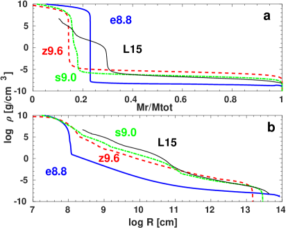
Figure 1: Density structure of the models e8.8, z9.6, s9.0, and L15 prior to the explosion. The top plot shows the density profiles versus mass coordinate relative to total mass. The bottom plot presents the same density profiles versus radius.

Table 1: Input models for our radiative transfer simulations. Note, that both the e8.8 and s9.0 stellar models are initially at solar metallicity, but the model e8.8 was computed with abundances from Asplund et al. (2009), having metallicity Z_⊙, and the model s9.0, taken from Sukhbold et al. (2016), was made with the assumption of solar abundances from Lodders (2003) having metallicity Z${}^{(1)}_{\odot}$. “Fe” stands for the mass fraction of stable iron in the stellar envelope. “E_kin” represents terminal kinetic energy of the entire ejecta. “Time” means time since bounce, i.e. the point where the models were mapped into STELLA, and approximately corresponds to time of the shock breakout. The comparison model L15 from Utrobin et al. (2017) is listed at the bottom as well.

	Mfin/Mej [$\mathrm{M}_{\odot}$]	Z	X(Fe)	R [$\mathrm{R}_{\odot}$]	Mcut [$\mathrm{M}_{\odot}$]	Time [days]	E${}_{\mathrm{kin}}^{\mathrm{fin}}$ [$10^{\,50}$ erg]	56Ni [$\mathrm{M}_{\odot}$]
e8.8 3D	5.83/4.5	Z⊙	4.7$\times 10^{\,-4}$	1200	1.326	5.2	0.86	0.0013
Tracer								0.0077
								0.0141
Z-study		0	0
		ZSMC	1.4$\times 10^{\,-4}$
Energy-study
3e49-2D							0.3	0.0009
6e49-2D							0.55	0.0011
1e50-2D							0.92	0.0013
1.5e50-2D							1.37	0.0012
Radius-study
e8.8 evol	5.82/4.5	Z⊙		1200	1.326		0.86	0.00092
e8.8 evol	4/2.7			900			0.86	0.00092
e8.8 evol	2.4/1.1			600			0.86	0.00098
e8.8 evol	1.8/0.5			400			0.86	0.00127
z9.6	9.6/8.25	0	0	214	1.353	5.8	0.81	0.0007
		ZSMC	1.4$\times 10^{\,-4}$
		Z⊙	5$\times 10^{\,-4}$
		Z${}^{(1)}_{\odot}$	1.4$\times 10^{\,-3}$
s9.0	8.75/7.4	Z${}^{(1)}_{\odot}$	1.46$\times 10^{\,-3}$	409	1.356	4.2	0.68	0.0051
L15-nu	15/13	Z${}^{(1)}_{\odot}$	1.36$\times 10^{\,-3}$	627	2	0	5.5	0.036
L15-tb	15/13.47	Z${}^{(1)}_{\odot}$	1.36$\times 10^{\,-3}$	627	1.53	0	5.4	0.036

We use three self-consistently modeled SN simulations as presented by Stockinger et al. (2020) for this study, namely, the ECSN model e8.8, and two low-mass CCSN models z9.6 and s9.0. e8.8 is a 1D solar-metallicity stellar evolution model which was constructed the following way before being mapped into the PROMETHEUS code: a 2.2 $\mathrm{M}_{\odot}$ core was initially calculated by Nomoto (1987). The envelope was computed with MESA (Jones et al., 2013), then truncated and attached to the core that was slightly reduced in mass (Nomoto & Leung, 2018; Leung et al., 2020). The reduced envelope mass is explained by the pre-collapse stellar evolution which contains numerous shell-burning flashes, i.e., pulsation-driven mass-loss episodes, and steady-state mass-loss (Poelarends et al., 2008). Furthermore, the available prescriptions for the mixing processes and mass-loss remain the overarching uncertainty in the final outcome of the models in the range between 8 $\mathrm{M}_{\odot}$ and 10 $\mathrm{M}_{\odot}$ (Jones et al., 2013). The final total mass of 5.83 $\mathrm{M}_{\odot}$ was chosen to match the estimated mass of the Crab Nebula (Hillebrandt, 1982; Nomoto et al., 1982; Tominaga et al., 2013). The model e8.8 is relatively physically large, having a radius of 1200 $\mathrm{R}_{\odot}$ which is similar to the average red supergiant. However, we show that the extended tenuous envelope makes the observational properties of this particular model quite unique.

Figure 2: Chemical structure (hydrogen, helium, carbon, and oxygen profiles) of the ejecta. Model designation as labeled. Dashed lines indicate the pre-collapse chemical structures of the models while solid lines present post-explosion structures.

Model z9.6 is a zero-metallicity stellar evolution model with initial mass of 9.6 $\mathrm{M}_{\odot}$ calculated with the KEPLER code (Weaver et al., 1978). With no metals in the original chemical mixture this model is relatively compact, its radius at the moment of iron-core collapse being 214 $\mathrm{R}_{\odot}$, i.e. the star is somewhere at the boundary between blue and red supergiants (Heger & Woosley, 2010). The solar-metallicity model s9.0 is a star with initial 9 $\mathrm{M}_{\odot}$ also produced with KEPLER (Sukhbold et al., 2016).

The choice of the models in the present study is explained by the following aspects:

1. One of the purposes of our study is to explore differences and similarities in the resulting supernova observables between models in the narrow range of initial ZAMS masses between 8 $\mathrm{M}_{\odot}$ and 10 $\mathrm{M}_{\odot}$.

2. Pre-collapse model e8.8 is the latest version of a super-AGB ECSN progenitor available to us.

3. The z9.6 progenitor has a density structure prior to the collapse similar to e8.8, namely, a steep density gradient at the core-envelope interface (see Figure 1).

4. Pre-collapse model s9.0 is the representative of low-mass progenitors and explodes fairly easily in self-consistent 3D simulations, having similar energy as the other two cases (see Radice et al., 2017; Glas et al., 2019; Stockinger et al., 2020).

We note that adding 3D simulations of more progenitors or more model variations is computationally expensive and currently not feasible. One of the reasons is the long time, up to 5 days, required for the shock to break out from these very extended progenitors. The approximate time for the shock breakout is definited as:

$$t_{\mathrm{SBO}}\sim 0.91~{}\mathrm{days}\,R_{500}\,E_{51}\,M_{10}\,,$$ (1)

where $R_{500}=R/500$ $\mathrm{R}_{\odot}$, $E_{51}=E_{\mathrm{exp}}/10^{\,51}$ erg, and $M_{10}=M_{\mathrm{ej}}/10$ $\mathrm{M}_{\odot}$ (see, e.g., Shigeyama et al., 1987; Goldberg et al., 2019). The macroscopic mixing processes proceed over this time. Consequently, the computational time is very long in order to catch all relevant dynamical effects.

These models were mapped into the PROMETHEUS code in order to simulate the contraction, bounce, shock formation, shock revival and shock propagation until the moment of shock breakout. The details of the simulations are fully described in the recent paper by Stockinger et al. (2020), therefore, we direct the reader to this comprehensive study for the details to avoid repetition.

In Table 1, we list relevant properties of the default models. Furthermore, we add the subsets of models we used for our study as explained in sections below. E.g. we did a “Tracer”-study for the model e8.8 in which we modified the mass of radioactive nickel ⁵⁶Ni according to the amount of so-called “Tracer” material (Section 3.6). We deem an exploration of metallicity dependence very important for the observational properties of our models. In order to do this, we constructed a subset of models for e8.8 by tuning the iron content in the hydrogen-rich envelope, either setting iron mass fraction to zero or to 0.00014, thus mimicking the zero-metalicity progenitor and the progenitor at Small Magellanic Cloud (SMC) metallicity. We did the same experiment for model z9.6, studying three additional metallicities: solar metallicity (set to 0.014 and 0.02 in accordance with Asplund et al. 2009 and Lodders 2003) and SMC metallicity (Section 3.4). For the model e8.8, we carried out an analysis of the influence of a different ratio between hydrogen and helium fraction in the outer envelope, as this ratio may differ taking the uncertainty of stellar evolution calculations into account (Section 3.5). We also carried out the radius-dependence study for e8.8, in which we produced 3 additional models with the radius of 400 $\mathrm{R}_{\odot}$, 600 $\mathrm{R}_{\odot}$, and 900 $\mathrm{R}_{\odot}$, while truncating the original 1D stellar evolution profile prior to the collapse.

In the current study, the models were mapped into the radiation hydrodynamics code STELLA (Blinnikov et al., 2006). This code is capable of processing hydrodynamics as well as radiation field evolution and computing light curves, spectral energy distribution and resulting broad-band magnitudes and colours. We used the standard parameter settings, well-explained in many papers involving STELLA simulations (see e.g., Kozyreva et al., 2019; Moriya et al., 2020).

We compare our radiative transfer results to the CCSN progenitor model L15 (Limongi et al., 2000; Utrobin et al., 2017), which is presented in Table 1 as L15-nu and L15-tb. We use this model as a “reference” CCSN model, even though the progenitors of CCSNe and their explosions are diverse. This model approximates the explosion of a massive progenitor with an initial mass of 15 $\mathrm{M}_{\odot}$ at solar metallicity, neglecting wind mass-loss (Limongi et al., 2000). We note though that the published light curves (Utrobin et al., 2017) mistakenly did not account for metallicity, i.e. there is no stable iron content in the hydrogen-rich envelope. We correct for this oversight in our calculations and figures. Even though there is a minor effect on the bolometric light curve, the bigger impact is observed for the U-band magnitude and colour temperature (see Section 3.4). The model’s final mass is thus the same as the initial mass, the resulting ejecta mass is 13.5 $\mathrm{M}_{\odot}$, and the radius at the moment of core-collapse explosion is 627 $\mathrm{R}_{\odot}$. For comparison, we used two types explosions for this model. The first explosion, named “L15-nu”, was done as a 3D neutrino-driven model with PROMETHEUS (Utrobin et al., 2017), i.e. the PROMETHEUS output was mapped directly into STELLA. The resulting light curve and observables are labelled “L15-nu” in the plots below. The second explosion, named “L15-tb”, was performed as a detonation of the progenitor L15 using the thermal bomb method, assuming an explosion energy of 0.9 foe (1 foe = $10^{\,51}$ erg) and reaching a terminal kinetic energy of 0.54 foe. The result of these simulations is labelled “L15-tb” in the plots below. The principal difference between a 3D neutrino-driven explosion and thermal bomb explosion lies in the absence of macroscopic mixing of the chemical composition in the latter case mapped into STELLA.

In Figure 2, we provide the input chemical profiles for the models in our study as well as the chemical structure of L15 for comparison. Dashed lines present pre-explosion chemical structures while solid lines present post-explosion distributions of hydrogen, helium, carbon and oxygen. The different chemical structures of the models is easily seen in the plot. The reference massive star model prior to the explosion exhibits a stratified chemical structure: the outer, hydrogen-rich, envelope rests on top of a thick 2 $\mathrm{M}_{\odot}$ pure helium shell, which in turn lies on an almost pure oxygen shell. In contrast, the low-mass model z9.6 has a thin 0.5 $\mathrm{M}_{\odot}$ helium layer and no oxygen layer, and the low-mass model s9.0 has no distinct helium shell at all. This is a result of macroscopic mixing occuring during the passage of the shock. At the same time the model L15 experiences macroscopic mixing and has the sharp chemical interfaces washed out to some degree. The ECSN model e8.8 exhibits a unique chemical structure, having only a hydrogen-rich envelope, polluted by a high fraction of helium and some amount of carbon and oxygen because of dredge-out episode, depending on metallicity. The very different chemical structure of the SN ejecta of these models leads to a variety of observational properties of the resulting SN light curves which we discuss in detail in the following sections.

Further, Figure 1 shows the pre-SN density structure prior to the collapse in order to illustrate the difference in the pre-explosion density profiles. The layers around the final neutron star in the model e8.8 look very unique compared to the other low-mass models (s9.0 and z9.6) and the reference CCSN model L15. The most important difference in model e8.8 is a very steep density gradient at the edge of the core culminating in a very tenuous hydrogen-rich envelope. The latter condition was shown by Grasberg & Nadezhin (1976) to prevent fast recombination in typical SN ejecta. The low-mass progenitors s9.0 and z9.6 differ from the reference massive progenitor. These models have no appreciable helium layer, while the reference massive star explosion L15 has a relatively massive helium shell ($0.19<M_{r}/M_{\mathrm{tot}}<0.3$) prior to the explosion. Apparently, the density structure is washed out after the passage of the shock. However, the shock propagation is different in these three different models and unavoidably influences a variety of properties of the ejecta and resulting observables.

3 Results

3.1 Bolometric properties

Figure 3: Bolometric light curves for the models e8.8, z9.6, s9.0, and L15-tb/L15-nu (Utrobin et al., 2017).

In Figure 3, bolometric light curves for the models explored in the current study are displayed. The bolometric light curves for the models e8.8 and z9.6 clearly differ from the canonical CCSN light curve, e.g. the curve labeled “L15-tb” and “L15-nu” from Utrobin et al. (2017). The difference consists in the sharp and pronounced drop between the plateau and the radioactive tail. The obvious explanation is that the models in our study produce too small amount of radioactive nickel ⁵⁶Ni, about 0.001 $\mathrm{M}_{\odot}$ (see Table 1). In contrast, the model s9.0 produces slightly higher amount of ⁵⁶Ni, about five times more (0.005 $\mathrm{M}_{\odot}$). Additionally the models e8.8 and z9.6 maintain their stratified structure even at the moment when all mixing processes cease. In contrast, there is significant large-scale mixing in the model s9.0. Concequently, the transition from the plateau to the radioactive tail is shallower in s9.0. The steepess of the transition in the models e8.8 and z9.6 is also caused by a lack of a distinct oxygen shell (Figure 2, Jones et al., 2013; Stockinger et al., 2020). As seen, the plateau luminosities for the low-mass CCSN models z9.6 and s9.0 are lower than that of a canonical CCSN originating from a standard mass progenitor, this is due to the relatively lower explosion energy. Nevertheless, the plateau luminostity for the ECSN model e8.8 is comparable to the normal CCSN as a result of the large radius of the progenitor ($L_{\mathrm{bol}}\sim R^{\,0.76}$, Goldberg et al. 2019).

Figure 4: Time evolution of the photospheric velocity, U_ph, for the models e8.8, z9.6, s9.0, and L15-tb/L15-nu.

In order to illustrate the overall energetics of the explosions, we show the photospheric velocity evolution for the models considered here together with the SN IIP reference models L15-nu and L15-tb in Figure 4. The photospheric velocity is the velocity of the mass shell in which the accumulated optical depth in B broad band is equal 2/3. It is easily seen that the photospheric velocity in all of our models, i.e. both the ECSN model and low-mass CCSN models, is systematically lower than the photospheric velocity for the reference SN IIP models L15-nu/L15-tb because of the lower explosion energy. Indeed photospheric velocity at the earliest phase is already very low, 2500 km s${}^{\,-1}$, while the reference CCSN model exhibits velocity of about 7000 km s${}^{\,-1}$, typical for observed SNe IIP (Jones et al., 2009). The photospheric velocity remains steady at a level of 1000–2000 km s${}^{\,-1}$ thoughout the entire plateau in all our models. However, the ECSN model exhibits roughly 500 km s${}^{\,-1}$ higher velocity during the plateau, i.e. slightly faster ejecta compared to the low-mass CCSN models in our study. This is explained by the fact of relatively lower ejecta mass. Velocity scales with energy $v\sim\sqrt{E/M}$, i.e. an increase a magnitude in energy (expected explosion energy for a ECSN is $10^{\,50}$ erg, while typical explosion energy of an CCSN is $10^{\,51}$ erg) leads to an increase in velocity about three times over, as seen in the plot. We suggest to use this diagnostic as a distinct feature in the identification of low-mass explosions, both ECSNe and low-mass CCSNe, which is in agreement with the suggestions by Pumo et al. (2017) and Tomasella et al. (2018).

3.2 Broad-band light curves and colours

We show the light curves in the standard Bessel broad-bands for the models e8.8, z9.6, and s9.0 in Figures 5, 6, and 7, respectively.

The broad-band light curves for the model e8.8 look similar to broad-band magnitudes for a reference SN IIP, excepting the first 50 days. The distinguishing feature of the model e8.8 is a 50-day blue plateau, i.e. the U band magnitude remains constant and even slightly increases over the first half of the plateau (see Figure 5), while normal SNe IIP usually exhibit a decreasing U-band magnitude across the entire plateau. We directly compare the U band magnitudes of the ECSN model and the CCSN model in the next section. We note that the original progenitor’s metallicity has a strong impact on the behaviour of the light curve in the U band, specifically, the higher metallicity leads to overall redder light curves (see e.g., Lentz et al., 2000). We explore the metallicity dependence in the Section 3.4 below. However, the model e8.8 shows blue colours even at solar metallicity. Reasons for this are the colour temperature evolution and the conditions during, and the time of, start of recombination (Grasberg et al., 1971; Goldfriend et al., 2014; Sapir & Waxman, 2017). In contrary to normal CCSNe, recombination settles in at relatively late times depending on the explosion energy (Shussman et al., 2016; Kozyreva et al., 2020a):

$$t_{\mathrm{rec}}\sim M^{\,0.22}R^{\,0.76}E^{\,-0.43}\,,$$ (2)

where $M$ is ejecta mass in 15 $\mathrm{M}_{\odot}$, $R$ is progenitor radius in 500 $\mathrm{R}_{\odot}$, and $E$ is explosion energy in 1 foe. The ejecta mass for ECSN progenitors is generally expected to be lower than that of CCSNe (e.g. for both our low-mass and the reference models). The explosion energy is also expected to be lower (see e.g., Melson et al., 2015; Radice et al., 2017; Stockinger et al., 2020). The progenitor radius of the ECSN e8.8 1200 $\mathrm{R}_{\odot}$ is significantly larger than the 214 $\mathrm{R}_{\odot}$ of model z9.6 (the latter being zero metallicity) and the 408 $\mathrm{R}_{\odot}$ of model s9.0. Note that the e8.8 radius is still in the range of reference progenitor radii of red supergiants (100 – 2850 $\mathrm{R}_{\odot}$, Levesque et al., 2005; Levesque et al., 2006). The larger radius of the ECSN progenitor (the super-AGB star), is a consequence the dredge-out episode (Nomoto, 1987; Ritossa et al., 1999; Jones et al., 2013). Accordingly, the hydrogen-rich envelope of the model e8.8 is very tenuous and recombination hard settles in, which in turn forces the overall electron-scattering photosphere to recede more slowly (Grasberg & Nadezhin, 1976).

The zero-metallicity model z9.6 demonstrates a quite unusual behaviour in the broad-band light curves compared to a normal SN IIP. We show in the next sections that the same model at solar metallicity should have colour behaviour quite standard for SNe IIP. Nevertheless, the zero-metallicity low-mass CCSNe, as demonstrated by the model z9.6, have monotonically rising U, B, V, R, and I light curves, and constant colours during the plateau phase. This means that the shape of the spectrum persists more or less unchanged for the first 100 days, i.e. while the electron-scattering photosphere gradually recedes through the hydrogen-rich envelope. Later, i.e. after the end of plateau, there is a sharp reddening of the colours. The photosphere at this phase enters the inner region of the ejecta dominated by iron-group elements which are the major contributors to the line opacity. However, compatible zero-metallicity stars (Population III) exist only in the early Universe, therefore, the application of model 9.6 is of limited usefulness, when observations in the nearby Universe are concerned. Predictions about observational properties of CCSNe for Population III stars are very useful for upcoming transient surveys like LSST (Whalen et al., 2013; Ivezić et al., 2019). However, the majority of known SNe IIP are found in non-zero metallicity galaxies (Anderson et al., 2016), and theoretical predictions for the observables of CCSNe at the SMC and solar metalicity are deemed more useful.

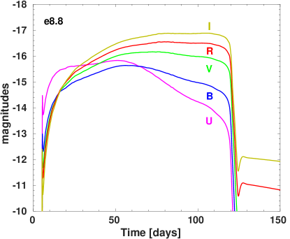
Figure 5: Broad-band U, B, V, R, and I light curves for the model e8.8.

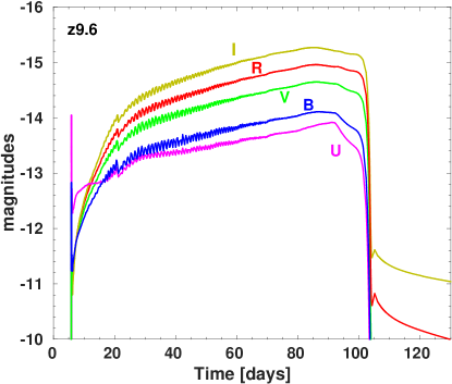
Figure 6: Broad-band U, B, V, R, and I light curves for the model z9.6.

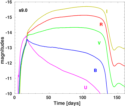
Figure 7: Broad-band U, B, V, R, and I light curves for the model s9.0.

3.3 Dependence on the explosion energy

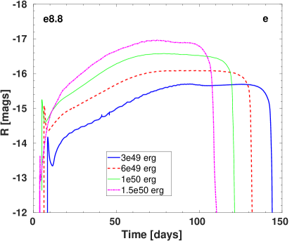
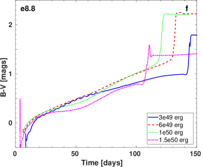
Figure 8: Dependence on the explosion energy: Bolometric, broad-band light curves, and B–V colour for the model e8.8 simulated in 2D and 3D with explosion energies as labelled.

The numerics and physics input in the core-collapse simulations lead to uncertainties in the final explosion energy (Radice et al., 2017; Melson et al., 2020). As a remedy, Stockinger et al. (2020) provided simulations for e8.8 with four different neutrino luminosity values in 2D corresponding to explosion energies of: $3\times 10^{\,49}$ erg, $6\times 10^{\,49}$ erg, $1\times 10^{\,50}$ erg, and $1.5\times 10^{\,50}$ erg (see Table 1). We would like to emphasize that the explosion energy is unequal to the terminal kinetic energy listed in Table 1. There are number of reasons for this difference. (1) The explosion energy published by Stockinger et al. (2020) is a direct integral of the total energy in 2D or 3D. The multidimensional profiles were converted into 1D-profiles using an angle-averaging procedure. (2) Since STELLA is a hydrodynamics code, it requires some numerical relaxation when mapping PROMETHEUS output into it, which in turn is liable to cause some (up to 15 %) difference in the resulting integrated energy. (3) The supernova ejecta at the moment of shock breakout have not yet reached the coasting phase. This causes some hydrodynamical evolution and inelastic conversion of kinetic energy into thermal energy. We note that the total mass of radioactive nickel ⁵⁶Ni is kept the same for different explosion energies. Nevertheless, it is expected that more energetic explosions naturally produce a higher mass of ⁵⁶Ni (Ertl et al., 2016). However, we find that the resulting chemical profiles in the post-shock ejecta structure do not differ significantly. For different energies the hydrodynamical profiles explicitly scale with the explosion energy. Otherwise, the final light curves obey the well-known Popov’s relation for absolute magnitude in V band and duration of the plateau $t_{p}$ (Litvinova & Nadezhin, 1985; Popov, 1993; Sukhbold et al., 2016; Goldberg et al., 2019):

$$V\sim-1.67\log R+1.25\log M-2.08\log E$$ (3)

$$\log t_{p}\sim 0.167\log R+0.5\log M-0.167\log E\,,$$

where $R$ is radius in $\mathrm{R}_{\odot}$, $M$ is ejecta mass in $\mathrm{M}_{\odot}$, and $E$ is explosion energy in foe. In Figure 8, bolometric and broad-band light curves and B–V colour for the model e8.8 computed with a variety of energies are presented. Figure 8a also shows the result of the simulations for the model e8.8 in 3D for an explosion energy of $1\times 10^{\,50}$ erg (bolometric light curve for the default model e8.8 is displayed in Figure 3). The light curves for this case are almost identical in 2D and 3D. This means that an explosion calculated in 2D provides the same hydrodynamical and chemical ejecta structure as in 3D. The higher explosion energy leads to a more luminous and shorter plateau. The broad-band magnitudes for this case follow the behaviour of the bolometric curve without major flux redistribution thoughout the spectrum. Figure 8 shows B–V colour for different choices in explsoion energy. There is no significant difference for cases of different energy. However, the colour tends to be slightly bluer for higher energies, e.g. B–V is 0.2 mag bluer an explosion energy of $1\times 10^{\,50}$ erg and $1.5\times 10^{\,50}$ erg in e8.8 at the end of plateau and later compared to the results for the lower explosion energy of $3\times 10^{\,49}$ erg and $6\times 10^{\,49}$ erg.

3.4 Dependence on the initial metallicity

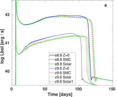
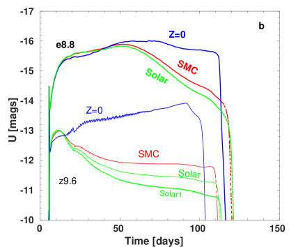
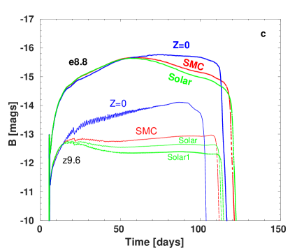
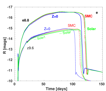
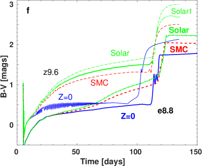
Figure 9: Dependence on the initial metallicity: Bolometric and broad-band light curves, and B–V colour for the subset of runs based on the model e8.8 and z9.6 with different stable-Iron content in the hydrogen-rich envelope, which corresponds to zero metallicity (“Z=0”), SMC metallicity (“SMC”), and solar metallicity (“Solar” and “Solar1”). “Solar” metallicity stands for the initial metallicity of the model e8.8 and has iron fraction of $5\times 10^{\,-4}$, while “Solar1” metallicity stands for the solar metallicity with the iron fraction of $1.4\times 10^{\,-3}$ (initial metallicity of the model s9.0).

In order to understand the influence of initial metallicity, we explored two of the models from the study in greater detail: e8.8 and z9.6. Specifically, we modified the stable iron abundance in the hydrogen-rich envelope. The subset of the runs for model e8.8 has the following adopted metallicity: zero ($Z=0$), SMC ($Z=0.0014$), solar ($X(\mathrm{Fe})=5\times 10^{\,-4}$), the latter being the default metallicity of the model e8.8). The subset of the runs for the model z9.6 has the adopted metallicity: zero ($Z=0$, the default metallicity of the input model), SMC ($Z=0.0014$, $X(\mathrm{Fe})=1.4\times 10^{\,-4}$), and two different runs for solar metallicity “solar” ($Z=0.014$, Asplund et al. 2009, $X(\mathrm{Fe})=5\times 10^{\,-4}$, the default metallicity of the model e8.8) and “solar1” ($Z=0.02$, Lodders 2003, $X(\mathrm{Fe})=1.4\times 10^{\,-3}$, the default metallicity of the model s9.0). Changing metallicity of the initial model unavoidably leads to different stellar evolution path, different mass-loss, consequently different final mass and progenitor radius (Georgy, 2012; Georgy et al., 2013; Jones et al., 2015; Renzo et al., 2017). We, nevertheless, rely on the conclusions we make based on the metallicity study we carried out in the frame of the current paper.

Iron is the most influencial element contributing to the overall line opacity. Therefore, light curves for runs with zero metallicity are significantly more blue than light curves for solar metallicity runs as seen in Figure 9 (see also Goldshtein & Blinnikov, 2020). The most significantly affected broad band magnitudes are U and B, while the V, R, and I magnitudes are less dependent on the iron content. This is due to the blue flux being effectively absorbed by iron and redistributed to longer wavelengths (Lucy, 1999; Kasen, 2006; Kozyreva et al., 2020b). Hence, a supernova may have a prominent 110-day plateau in U and B broad band in case of zero metallicity (e8.8 at $Z=0$), while having a 50 day plateau with a subsequent decline in case of solar and SMC metallicity (e8.8 “solar” and e8.8 “SMC”). Interestingly, the U broad band light curve rises for the model z9.6 with the default zero metallicity, while it declines for solar/solar1 and SMC metallicity, similar to many typical SNe IIP. Similarly, the light curve rises in B band in case of zero metallicity, while the model z9.6 shows a plateau in B if the iron content in the hydrogen-rich envelope corresponds to solar or SMC metallicity. Hence, the U band light curve serves as a direct indicator of the initial metallicity of the progenitor for CCSNe (Dessart et al., 2013; Dessart et al., 2014). The same is true for the ECSN model e8.8. However, the earlier 50-day U band light curve remains unaffected by metallicity, because of the relatively long delay until recombination settles in (see Figure 5). Additionally, metallicity, i.e. iron content in the hydrogen-rich envelope, effectively determines the length of the plateau. Specifically, a difference of 5 to 10 days is observed in duration of the plateau between runs with zero and solar/SMC metallicity: the higher metallicity the longer the plateau (see e.g., Kasen & Woosley, 2009).

3.5 Dependence on the H-to-He-ratio in the outer envelope

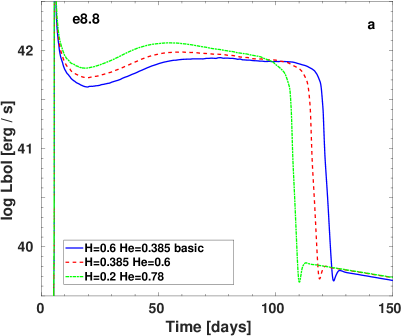
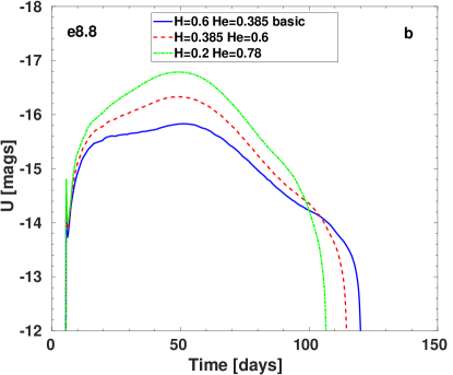
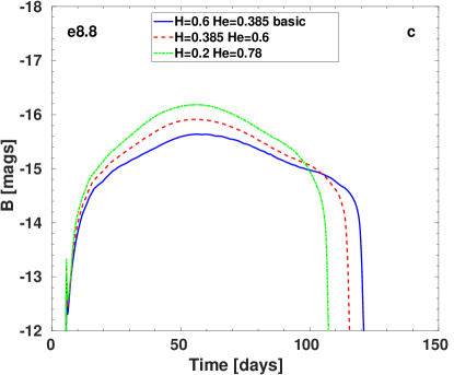
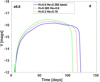
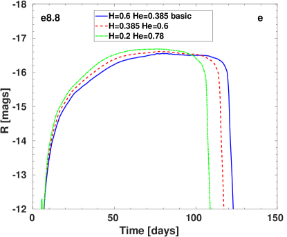
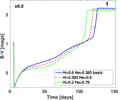
Figure 10: Dependence on the hydrogen-to-helium-ratio: Bolometric and broad-band light curves, and the B–V colour for the subset of runs based on the model e8.8 with different hydrogen-to-helium-ratio: 0.385:0.6, 0.385:0.6, and 0.2:0.78.

Different works (e.g., Nomoto, 1987; Ritossa et al., 1999; Siess, 2007, and other studies) report that one of the distinct properties of the evolution of stars in the narrow mass range around 8 $\mathrm{M}_{\odot}$, is a sequence of carbon-shell burning flashes which lead to the dredge-out episode. This later results in complete destruction of the helium layer and macroscopic injection of helium into the hydrogen-rich envelope. The stellar models consequently tend to have a decreased hydrogen-to-helium ratio in the envelope (see, however, Woosley & Heger 2015). Tominaga et al. (2013) explored the consequence of different hydrogen-to-helium ratios on SN light curves. In their study, the relative hydrogen abundance in the envelope was set to 0.7, 0.5, and 0.2. We carried out a similar study, this time assuming two different hydrogen abundances in addition to the default value: 0.385 and 0.2 (the default value of the hydrogen abundance is 0.6). The resulting light curves are shown in Figure 10. The impact of a different hydrogen-to-helium ratio is the same as found by Tominaga et al. (2013) and similar to that found by Kasen & Woosley (2009) for normal SNe IIP. The lower hydrogen abundance leads to a slightly shorter and brighter plateau. This is explained by the lower electron abundance, in this case. The lower electron abundance leads to a lower electron-scattering opacity which governs the dynamics of the receding photosphere. According to Nomoto et al. (1982), the hydrogen-to-helium ratio in the Crab nebula, which is believed to originate from an ECSN explosion, ranges between 0.125 and 0.625 with the hydrogen fraction in the range 0.2–0.3. Therefore, the green light curves in Figure 10 are more favourable for this ECSN candidate. The B–V colour differs not significantly between variants of e8.8 with different hydrogen-to-helium ratio, showing a scatter of 0.2 mag during the plateau phase. Otherwise the behaviour of the light curves with different hydrogen-to-helium ratios is similar.

3.6 Dependence on the assumed yield of the Tracer material

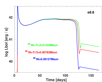
Figure 11: Bolometric light curves for the subset of runs based on the model e8.8 with different ⁵⁶Ni mass: “pure” ⁵⁶Ni, ⁵⁶Ni+Tracer/2, and ⁵⁶Ni+Tracer, which correspond to 0.00127 $\mathrm{M}_{\odot}$, 0.00783 $\mathrm{M}_{\odot}$, and 0.01435 $\mathrm{M}_{\odot}$.

The core-collapse explosion simulations for our models were carried out with the PROMETHEUS code, which provides a small 23-isotope (VERTEX-PROMETHEUS) and a 16-isotope (PROMETHEUS-HOTB) nuclear network (for details, see Stockinger et al., 2020). The production of iron-group elements in those studies is governed by the reduced set of nuclear species used in the treatment of nuclear statistical equilibrium and in a simplified nuclear alpha-reaction network. The latter provides an approximate estimate of the ⁵⁶Ni yield. However, the exact amount of ⁵⁶Ni depends on the electron fraction (or neutron-to-proton ratio) in the ejecta, which is not accurately determined with the approximate neutrino transport used in the PROMETHEUS-HOTB simulations of the model e8.8. In neutron-rich conditions (electron fraction $Y_{e}<0.49$) the code produces a so-called “tracer” nucleon that traces neutron-rich nuclei. With more accurate $Y_{e}$, some fraction of this tracer could actually be radioactive nickel ⁵⁶Ni. To account for this uncertainty, we run two additional simulations for the same hydrodynamical profile of the default model e8.8 for which we set the ⁵⁶Ni yield to be the following: ${}^{56}\mathrm{Ni}+\mathrm{Tracer}/2$ and ${}^{56}\mathrm{Ni}+\mathrm{Tracer}$. We show the result of the simulations in Figure 11. Different total amounts of radioactive nickel ⁵⁶Ni with the same shape of distribution throughout the ejecta largely affect the luminosity of the radioactive tail and the extension of the plateau (Kozyreva et al., 2019). Inclusion of the entire mass of the Tracer into the ⁵⁶Ni mass leads to higher mass of the radioactive material, i.e. reduces the drop between the plateau and the tail, and makes the ECSN bolometric light curve more similar to that of normal SN IIP of a massive progenitor (10 – 20 $\mathrm{M}_{\odot}$). However, the overall spectral evolution and colours remain the same as for the default model e8.8.

3.7 Dependence on the progenitor radius. The case of e8.8

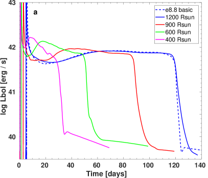
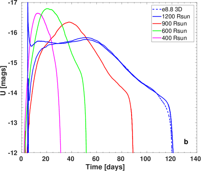
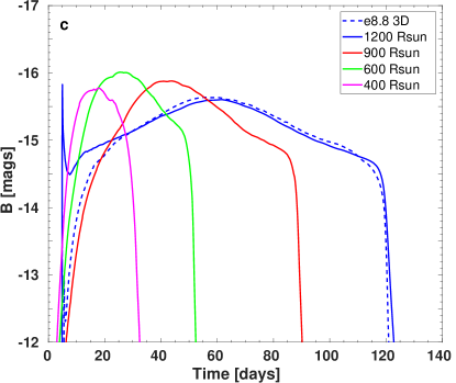
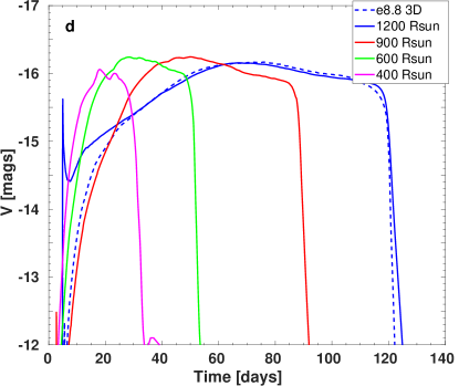
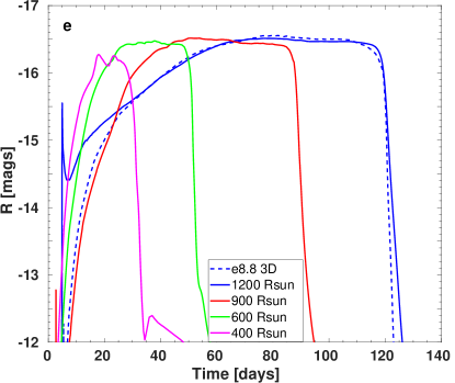
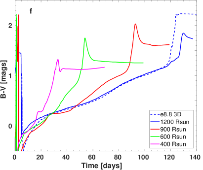
Figure 12: Bolometric light curves for the subset of runs based on the stellar evolution model e8.8 with different degree of truncated envelope.

It is known that the large fraction of stars are born in binary, triple or multiple systems (Podsiadlowski et al., 1992). Similar to the famous Algol paradox, stars lose its mass via critical Roche surface (Pustylnik, 1998). The stellar evolution of individual stars is strongly affected if they are part of a close binary. Therefore, it is adequate to admit some degree of uncertainty to the mass-loss. Additional mass-loss happens via mass transfer in a binary system, which is the channel for some initially hydrogen-rich low-metallicity massive stars to result in hydrogen-free supernovae SN Ib/c (Yoon et al., 2012). Georgy (2012) show that increasing the wind mass-loss rate by a factor of 3 to 10 shrinks the progenitor, i.e. makes the more compact star. Multipling the rate of wind mass-loss may mimic the binarity, i.e. the enhanced mass-loss happening in a binary via Langrangian point L1. Specifically, ECSNe may occur in binaries (Eldridge et al., 2008; Poelarends et al., 2017; Siess & Lebreuilly, 2018). Tauris et al. (2015) and Jones et al. (2019a) show that a star that would otherwise result in an ECSN will instead result in an ultra-stripped SN if part of a close binary. Losing mass via close binary interaction, i.e. via the Roche lobe overflow, a star becomes more compact. Hence, we did additional subset of runs based on the stellar evolution model e8.8 which has radius of 1200 $\mathrm{R}_{\odot}$ at the moment of collapse. Three another truncated models have radii of 900 $\mathrm{R}_{\odot}$, 600 $\mathrm{R}_{\odot}$, and 400 Rsun. We note that the main model e8.8 discussed above was evolved with PROMETHEUS up to the moment of shock breakout and then was mapped into STELLA. Truncating the main profile (the PROMETHEUS output) leads to cut in the total energy budget. Therefore, we used the stellar evolution 1D output which was mapped into PROMETHEUS prior to the collapse. We detonate it with the thermal bomb method with according explosion energy. We note that the amount of explosion energy was set in a way to allow the subset models to reach the same terminal kinetic energy of 0.86$\times\,10^{\,50}$ erg which is the explosion energy of the main model e8.8 in the study. The reduction of the radius by cutting numerically leads to some degree of inconsistency, since the star is supposed to relax into a new thermodynamical equilibrium. Another unavoidable side-effect consists in reduction of the ejecta mass. Hence the total mass for the truncated sub-models are: 1.8 $\mathrm{M}_{\odot}$, 2.4 $\mathrm{M}_{\odot}$, 4 $\mathrm{M}_{\odot}$ for 400 $\mathrm{R}_{\odot}$, 600 $\mathrm{R}_{\odot}$, and 900 $\mathrm{R}_{\odot}$ cases, respectively.

In Figure 12, the resulting bolometric, broad-band light curves and the B-V colour are shown. The artificially detonated stellar evolution model (labelled “1200 Rsun”) displays the same curve as the main model e8.8 exploded in a self-consistent manner (blue solid and dashed curves). There is some difference between these curves due to a few reasons. First, the detonated evolutionary model does not have any applied macroscopic mixing of chemicals. Second, PROMETHEUS simulations were performed without taking radiation transport into account while STELLA does hydrodynamics coupled with radiation transport. I.e. this leads to a difference in propagation of the radiation-dominated shock. Third, PROMETHEUS does not include heating from radioactive ⁵⁶Ni, while STELLA does. The presence of ⁵⁶Ni results in variation in velocity, temperature and density field which is called “Ni-bubble” effect and leads to variation in, e.g., velocity upto 10 – 15 % in the region where ⁵⁶Ni mass fraction is close to unity (Kozyreva et al., 2017). Fourth, the PROMETHEUS 3D output was angle-averaged to be suitable for mapping into STELLA which leads to the slight variation in hydrodynamical profiles and may cause some diversity in the resulting radiation transfer simulations.

As seen in Figure 12, the more compact the progenitor the shorter the plateau, which is consistent with Equation 3 (Popov, 1993) and numerical experiments by Young (2004). However, the plateau duration has the major impact from the ejecta mass which is connected to the reduction of the radius. The model e8.8 being truncated to 400 $\mathrm{R}_{\odot}$ has a very short living light curve lasting only 30 days, although it still retains hydrogen-rich envelope with the total mass of hydrogen of 0.3 $\mathrm{M}_{\odot}$. The colour of the more truncated models tends to be bluer since the hotter region of the ejecta gets closer to the outer edge. The higher temperature also explains the bump in the bolometric light curves for the cases of 400 $\mathrm{R}_{\odot}$ and 600 $\mathrm{R}_{\odot}$. For the same reason U-band light curves for the 400 $\mathrm{R}_{\odot}$ and 600 $\mathrm{R}_{\odot}$ cases are relatively luminous. We conclude that ECSNe in the binaries have fastly declining low-luminosity light curves and will be easily missed even being exploded in the close vicinity. This is the reason that there is no solid detection of an ECSN yet.

4 Comparison to a normal SN IIP model

U and V broad-band light curves for three default models from our study and the reference CCSN model L15-nu/L15-tb are shown in Figure 13. The U magnitude of the model z9.6 evolves significantly differently to other models due to its lack of metals. We study the effect of metallicity and discuss our results in Section 3.4 above. The light curves of L15-tb and L15-nu in U-band decline 2 mags during 50 days, i.e. evolves typically for the canonical SNe IIP. s9.0 U-band light curve behaves the same way as the reference CCSN model L15-nu/L15-tb with a systematically lower luminosity overall. There is no appreciable difference between plateau-like light curves in V band for the ECSN model e8.8 and the low-mass CCSN models z9.6 and s9.0 in comparison to the reference CCSN model L15-nu/L15-tb.

The colours B–V, V–R, and V–I are bluer for z9.6 and e8.8 compared to the models s9.0 and L15-nu/L15-tb. This is a conquence of the lack of metals in the model z9.6 and the unusual colour temperature evolution for the model e8.8. We discuss the latter below.

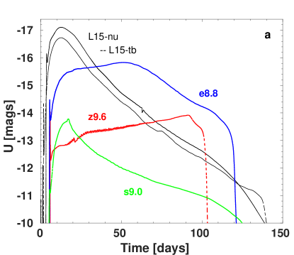
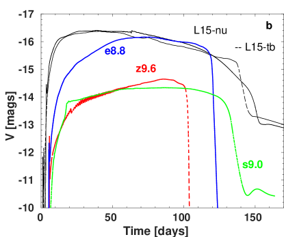
Figure 13: U and V broad-band light curves for the models e8.8, z9.6, s9.0, and L15-nu/L15-tb.

The colour temperature evolution for all models is shown in Figure 14. The colour temperature is the black body temperature as estimated from the least-square method. It serves as the indicator of the maximum in the spectral energy distribution, i.e. represent the frequency where the major flux is radiated. As was discussed above, recombination sets in at relatively late times in the model e8.8 compared to the other models. This is explained by a strong dependence of the “recombination time” on the radius of the progenitor and energy of the explosion (see Equation 2). The distinguishing property of ECSN progenitors is the large radius, and generally ECSN explosions are low energetic, therefore, the recombination time tends to be relatively long. Specifically the radius of model e8.8 is 1200 $\mathrm{R}_{\odot}$, quite large even for an average red supergiant. The explosion energy of the reference explosion model e8.8 is 0.1 foe. According to Equation 2 (Shussman et al., 2016; Kozyreva et al., 2020a), recombination is established at day 66 for the model e8.8, day 22 for the models z9.6 and L15, and at day 38 for the model s9.0.

Hence the main feature which distinguishes ECSN explosions from CCSN explosions are the behaviour of the blue flux, i.e. U and B magnitude, colour temperature, and colours. The specific features of e8.8’s observables are:

1. the light curve in the U and B bands rising during the first 50 days and then slowly declining,

2. the light curve in V and other redder bands rising during the same phase of 50 days and then holding at a plateau before the sharp drop to the low-luminosity tail powered by a small amount of the radioactive nickel ⁵⁶Ni.

We emphasise that this unique behaviour is the consequence of the relatively extended hydrogen-rich envelope and the absence of helium and oxygen shells which in turn is the result of the unique stellar evolution path of the super-AGB stars (see e.g., Doherty et al., 2015).

The main differences between low- and normal-mass CCSNe are (1) an overall lower luminosity at the plateau, 0.5 – 1 dex for bolometric luminosity or 1.5–2 mags in V broad band, (2) a low-luminosity radioactive tail, and (3) a large drop in luminosity between the plateau and the tail. All of these features are explained by the relatively lower explosion energy of low-mass explosions (below 0.1 foe) and a lower yield of radioactive nickel.

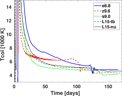
Figure 14: Colour temperature evolution for the models e8.8, z9.6, s9.0, and L15-nu/L15-tb.

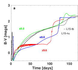
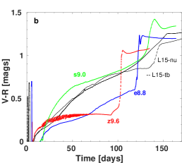
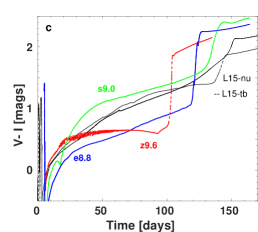
Figure 15: B–V, V–R, and V–I colours for the models e8.8, z9.6, s9.0, and L15-nu/L15-tb.

5 Application to observations

In this section we consider the results of our radiative transfer simulations for the ECSN model e8.8 and the low-mass CCSN models z9.6 and s9.0 in the context of observations. Particularly, we aim to find possible candidates matching our calculations. Further, we aim to point out the criteria for distingushing properties, specifically for the ECSNe and low-mass CCSNe. Immediately we encounter an obvious problem: namely that the number of detected and followed-up SNe increases every year at an exponential rate (Gal-Yam et al., 2013). Therefore, in our analysis we opt to compare our synthetic light curves to a representative sample and draw some general conclusions.

5.1 SN 2005cs

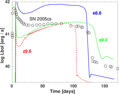
Figure 16: Bolometric light curves for the models e8.8, z9.6 and s9.0 and observed SN 2005cs (Pastorello et al., 2009).

For example, low-mass CCSNe are expected to be low energy and to produce a small amount of ⁵⁶Ni leading to a low-luminosity plateau, and a large drop towards the low-luminosity radioactive tail. Therefore, we choose SN 2005cs as the first example for our comparison. This event is famous for its low plateau luminosity and steep and pronounced drop towards the tail. We show the bolometric light curve of SN 2005cs (Pastorello et al., 2009) superposed on our simulated bolometric light curves in Figure 16. It is apparent that none of the models match the bolometric light curve of SN 2005cs. However, there are some conclusion to be drawn on the general energetics and bolometric parameters of this particular SN and its possible progenitor. (1) SN 2005cs is likely not a ECSN explosion with an envelope and energy as model e8.8, because the luminosity of the SN throughout the plateau phase is about 0.2–0.5 dex lower than the luminosity of the ECSN model e8.8. This means that the progenitor of SN 2005cs was likely more compact than our model (with a radius of 1200 $\mathrm{R}_{\odot}$), which is in agreement with the conclusion drawn by Eldridge et al. (2007). (2) The model s9.0 is likely more similar to the real progenitor of SN 2005cs. The remaining differences are explained either by the radius of the progenitor larger than the radius of the model s9.0 (408 $\mathrm{R}_{\odot}$) or/and the explosion energy being higher than $0.7\times 10^{\,50}$ erg. The total mass of the radioactive ⁵⁶Ni in SN 2005cs is likely lower than the 0.005 $\mathrm{M}_{\odot}$ contained in the model s9.0. Pastorello et al. (2009) proposed the following parameters for the progenitor based on their simulations: radius 100 $\mathrm{R}_{\odot}$, ejecta mass 11.1 $\mathrm{M}_{\odot}$, and explosion energy $3\times 10^{\,50}$ erg. Later Spiro et al. (2014) revised these numbers providing new parameters for SN 2005cs: 350 $\mathrm{R}_{\odot}$, 9.5 $\mathrm{M}_{\odot}$, and 1.6$\times 10^{\,50}$ erg. The photospheric velocity of SN 2005cs is at the same level as in our models (Figure 4), i.e. about 1000–2000 km s${}^{\,-1}$. Hence, judging from the bolometric properties of the SNe, the progenitor is likely a low-mass star of moderate radius which exploded at relatively low energy, but still higher than the low energy explosions in our study.

We show the broad-band magnitudes of the model s9.0 and SN 2005cs in Figure 17. As discussed in the previous sections, U magnitude is a very unique indicator of many model parameters, such as iron and nickel content in the ejecta and the radius of the progenitor. From the plot, we conclude that the model s9.0, which is the most similar to a normal SN IIP judging from its U band light curve, still evolves too shallowly. On the one hand, this is explained by the fact that radioactive nickel is mixed extensively in the ejecta of s9.0, retaining flux in the blue bands to later times. On the other hand, increased short wavelength flux might be explained by a low stable iron content in the hydrogen-rich envelope. However, as the model s9.0 is computed with solar metallicity, and the contained iron is able to absorb the blue flux sufficiently. There are a few assumptions, e.g. using a super-solar metallicity model or reducing the mass and/or radius of the existing s9.0 model, which might result in the recombination wave receding faster (i.e. U magnitude to decline sharper). Magnitudes in V, R, and I bands tend to rise after day 20, while observed SNe, particularly normal SNe IIP or other low-luminosity SNe (as seen in Spiro et al. 2014), have light curves declining in broad-bands B and V, or exhibit a plateau in R and I.

There is another distinct feature seen in Figure 17: observed magnitudes have an significant flux excess compared to the synthetic light curves of the model s9.0. This may indicate that the true progenitor is more extended than the model s9.0. However, introducing a larger progenitor radius unavoidably leads to higher luminosity during the plateau phase (Popov, 1993).

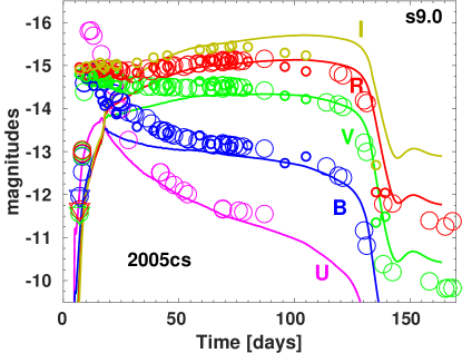
Figure 17: Light curves for the model s9.0 and observed SN 2005cs in broad bands Small and large circles correspond to the observed data taken from Tsvetkov et al. (2006) and Pastorello et al. (2009), respectively. Triangles present the upper limits for observed magnitudes.

5.2 SN 1999br

A number of low-luminosity SNe IIP have been observed (Pastorello et al., 2004; Spiro et al., 2014). We show a comparison of broad-band light curves of the model s9.0 to one of these SNe (SN 1999br) in Figure 18. The distance to the parent galaxy of SN 1999br (NGC 4900) is subject to uncertainty. We apply the up-to-date distance modulus from Karachentsev & Karachentseva (2019). Accordingly, the magnitudes for all observed broad-band magnitudes are well matched by the model. However, there is a flux excess at earlier time which suggests similarity between SN 1999br and SN 2005cs. Another reason for the luminosity excess at earlier time may lie in the possibility of interaction of the SN ejecta with the circumstellar matter, expelled by the progenitor as wind during earlier evolutionary stages (Morozova et al., 2017; Moriya et al., 2018; Goldberg & Bildsten, 2020). However, adding a wind environment to the model leads to certain consequences for observations. In particular, the SN can be expected to exhibit an X-ray excess which is not observed for every SN IIP.

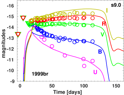
Figure 18: Light curves for the model s9.0 and observed SN 1999br in broad bands (Pastorello et al., 2004).

The low-luminosity SN 2008bk is considered to be similar to SN 1999br in its photometric evolution (Van Dyk et al., 2012). According to Lisakov et al. (2017), SN 2008bk is best fitted by a progenitor of initial mass 12 $\mathrm{M}_{\odot}$ (model X in their study), pre-explosion radius 502 $\mathrm{R}_{\odot}$ (consistent with 496 $\mathrm{R}_{\odot}$ derived by Pastorello et al. (2004) and 500 $\mathrm{R}_{\odot}$ by Pumo et al. (2017)), ejecta mass of 8.29 $\mathrm{M}_{\odot}$, ejected ⁵⁶Ni mass of 0.0086 $\mathrm{M}_{\odot}$, and explosion energy $2.5\times 10^{\,50}$ erg. However, Lisakov et al. (2017) state that this energy is too high to match photospheric velocity evolution (see also Lisakov et al., 2018). In contrast, our model s9.0 fits the observed velocity better due to a significantly lower explosion energy of $0.68\times 10^{\,50}$ erg and a lower ejecta mass of 7.4 $\mathrm{M}_{\odot}$ ($E/M=0.092$ in our study versus 0.3 in Lisakov et al. (2017)). Similarly, SN 1997D was explained by Chugai & Utrobin (2000) as a low-mass (6 $\mathrm{M}_{\odot}$) low energetic explosion ($1\times 10^{\,50}$ erg).

5.3 SN 2018zd and SN 2018hwm

It is worth mentioning that recently Zhang et al. (2020) and Hiramatsu et al. (2020) presented evidence of SN 2018zd as an ECSN candidate. However, the evolution of the broad-band magnitudes, specifically, the decline of the U band magnitude, is very similar to an average SN IIP. An analysis of spectra (FLASH-spectroscopy) and the time evolution of the photospheric velocity also indicate the explosion of an average massive star in a surrounding wind (Zhang et al., 2020). Hence, the most probable explanation is that SN 2018zd was a low- to intermediate-mass iron-CCSN. Note that the distance to the host galaxy (NGC 2146) is estimated two times larger by Zhang et al. (2020) than by Hiramatsu et al. (2020), which directly affects all consequently derived values of the explosion energy, the mass of radioactive nickel ⁵⁶Ni, radius of the progenitor and other parameters. Specifically, Zhang et al. (2020) estimate 0.033 $\mathrm{M}_{\odot}$ of ⁵⁶Ni while Hiramatsu et al. (2020) calculate 0.0086 $\mathrm{M}_{\odot}$ of ⁵⁶Ni. Particularly, the latter conclude that SN 2018zd was an ECSN based on the low mass of ⁵⁶Ni. Nevertheless, it is difficult to discriminate different kinds of progenitors relying on the estimated ⁵⁶Ni mass, because the amount of ⁵⁶Ni produced during neutrino-driven explosions is mostly a function of the explosion energy (Sukhbold et al., 2016; Ertl et al., 2020), and both ECSNe and low-mass iron-CCSNe can explode with similar energies.

Moreover, Reguitti et al. (2021) observed the low-luminosity SN 2018hwm and suggested two possibilities: either it is an ECSN or a low-mass iron-CCSN. The authors do not favour one possibility over the other. However, a low plateau luminosity does not necessarily indicate an ECSN candidate, i.e. an explosion of a super-AGB star, because the luminosity depends on the radius, and the radius of an ECSN progenitor might be very large. E.g. our extended ECSN progenitor e8.8 exhibits a luminosity on the plateau of about $9\times 10^{\,41}$ erg s${}^{\,-1}$, i.e. comparable to an average SN IIP (Hamuy & Pinto, 2002; Pejcha & Prieto, 2015; Müller et al., 2017), as we show in Figure 3. On the other hand, the very low photospheric velocity of about 1500 km s${}^{\,-1}$ and very long plateau of 150 days explicitly point to a low explosion energy, 0.055 foe, as derived by Reguitti et al. (2021). The very low mass of radioactive nickel ⁵⁶Ni of 0.002 $\mathrm{M}_{\odot}$ also does not necessarily point the explosion as an ECSN, because our low-mass iron-core explosions produce as little ⁵⁶Ni as 0.0007 $\mathrm{M}_{\odot}$ (model z9.6, see Table 1). Therefore, SN 2018hwm is also most likely a low-mass iron-CCSN.

To conclude, the published observations cannot exclude low-mass iron-CCSNe as an explanation of SN 2018zd and SN 2018hwm.

5.4 B –V colour diagnostics

In Figure 19, we show the B–V colour for our models e8.8, z9.6, and s9.0, in comparison to five normal SNe IIP, namely the typical SN 1999em, and also SN 2013fs, ASASSN 2014gm, ASASSN 2014ha, SN 2005cs (Pastorello et al., 2009; Faran et al., 2014b, a; Valenti et al., 2016). As mentioned by Kozyreva et al. (2019), the B–V colour could serve as an indicator of the ⁵⁶Ni mixing in the SN ejecta. Indeed, the models e8.8 and z9.6 have a strictly stratified chemical structure, leading to a sharp reddening at the end of the plateau, while the model s9.0 has extensive mixing of radioactive nickel in the ejecta. Extensive mixing of radioactive nickel leads to colour reddening more gradually at the end of the plateau. Still, none of the models in our study matches the behaviour of the B–V colour for the typical SNe IIP in our sample. It is possible that the model s9.0 might explain the colour of SN 2005cs while having a smaller mass of ⁵⁶Ni. With 0.005 $\mathrm{M}_{\odot}$ of ⁵⁶Ni the colour reddens to much after the transition to the tail, meaning the absorption, i.e. line opacity, is very strong in the inner ejecta.

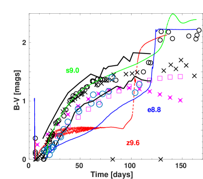
Figure 19: The B–V colour for the models e8.8, z9.6 and s9.0 and observed SN 1999em, SN 2013fs, ASASSN 2014gm, ASASSN 2014ha. We also superpose the lower and upper limits for the B–V colour for normal SNe IIP derived by Faran et al. (2014a) represented by black lines.

Contrary to the conclusions of Botticella et al. (2009), the light curve of SN 2008S is dissimilar to the ECSN model e8.8. The distinguishing property of an ECSN, i.e. a super-AGB progenitor explosion, is not a low-luminosity plateau, but a distinct moderate luminosity plateau accompanied by a sharp transition to a low-luminosity radioactive tail. Tominaga et al. (2013) also speculate that SN 2008S is most likely not an ECSN explosion. However, they suggest that a more compact ECSN progenitor might be a good candidate for SN 2008S, especially taking the uncertainty of the wind mass-loss and pulsationally-driven mass-loss into account.

The sub-class of very faint, faint, or/and low-luminosity SNe IIP (Pastorello et al., 2004, 2007; Spiro et al., 2014) are most likely explosions of low-mass progenitors, similar to our model z9.6 but at solar metallicity and a lower energy, e.g. a few $10^{\,49}$ erg, and relatively low masses of ejected ⁵⁶Ni. The very low energies of these explosions are favoured by the low photospheric velocity during the plateau phase.

6 Conclusions

In this study, we present the evolution of the SN ejecta of three progenitors: the ECSN progenitor e8.8, the low-mass zero-metallicity z9.6, and the low-mass solar-metallicity s9.0, with initial ZAMS masses of 8.8 $\mathrm{M}_{\odot}$, 9.6 $\mathrm{M}_{\odot}$, and 9 $\mathrm{M}_{\odot}$, respectively. The models were exploded self-consistently with PROMETHEUS by Stockinger et al. (2020). We calculated the hydrodynamical evolution and radiative transfer simulations for these three models with STELLA. The resulting light curves differ from explosions of massive stars. We used 15 $\mathrm{M}_{\odot}$ model L15 (Limongi et al., 2000) as a reference CCSN model for comparison. Among the reasons for the differences are:

• low explosion energy;

• low mass of ejected radioactive nickel ⁵⁶Ni;

• absence of the distinct massive ($>1$ $\mathrm{M}_{\odot}$) helium shell and oxygen layer.

The distinct properties of the SNe arising from our default models can be summarised as:

The model e8.8:

• during the first 50 days: plateau in U band and rising magnitudes in B, V, R, and I bands.

• after day 50: plateau in R and I bands.

• the transition to the tail is steep and pronounced, more than two orders in bolometric luminosity, or 6 mags in V band.

• colour temperature remains above 6000 K until the middle of the plateau.

The model z9.6:

• relatively low luminosity on the plateau, $\log L_{\mathrm{bol}}\sim 10^{\,41}$ erg s${}^{\,-1}$, or –14.5 mags in V band.

• pronounced and steep transition to the tail, about 1.5 orders in bolometric luminosity, or 4.6 mags in V band.

• magnitudes in all broad bands increase starting at early times. The colours remain largely constant during the plateau phase.

The model s9.0:

• relatively low luminosity during the plateau phase, $\log L_{\mathrm{bol}}\sim 10^{\,41}$ erg s${}^{\,-1}$, or –14 mag in V band.

• shallow transition to the tail due to extended macroscopic mixing of radioactive material.

• the transition is less pronounced, about 3.5 mags in V band.

The model s9.0 is the best candidate among our models for the observed low-luminosity SNe IIP according to its broad-band light curves and colour evolution.

For all our models, photospheric velocity is relatively low, 1000 – 2000 km s${}^{\,-1}$ during the plateau. This feature is a convenient indicator of low-mass explosions.

We do not find a good candidate among our sample of observed SNe resembeling the observables of the ECSN model e8.8. According to our models, low-luminosity SNe IIP like SN 1999br and SN 2005cs, can be explained by the explosion of low-mass CCSNe. However, the observed SNe show a clear flux excess at the earlier phase (before day 20). This requires either more extended progenitors or the presense of circumstellar matter (e.g. pre-SN wind), and interaction of the SN ejecta with the circumstellar environment.

Further we carried out the following studies:

1. Variations of the ⁵⁶Ni mass produced in model e8.8. The more ⁵⁶Ni is ejected, the longer is the plateau and the higher the luminosity on the tail. Slightly bluer colours (0.2 mags in B–V).

2. Variations of the explosion energy for the model e8.8. We find that the light curves obey the standard relations from Popov (1993), i.e. the higher the energy the shorter and brighter the plateau. Slightly bluer colours (0.2 mags in B–V).

3. Variations of the hydrogen-to-helium ratio in the model e8.8. Here we find that the higher helium fraction in the hydrogen-rich envelope, the shorter and brighter the plateau. Slightly bluer colours (0.2 mags in B–V).

4. A metallicity study for the models e8.8 and z9.6. We find that the higher the metallicity, i.e. the higher the iron abundance in the hydrogen-rich envelope, the redder the colours; the U band magnitude is good indicator for measuring the metallicity of the SN progenitor; the B–V colour changes significantly: 1 mag between zero metallicity case and SMC/solar metallicity.

5. A radius-dependence study for the ECSN model e8.8. Assuming the ECSN explodes in a binary system, the progenitor may lose hydrogen-rich envelope via close binary interaction. We found out that the light curves for the truncated models become shorter, namely, the sub-model with the radius 400 $\mathrm{R}_{\odot}$ has the sharply declining 30 day light curve with a low-luminosity maximum phase. Therefore, ECSNe in binaries are mostly undetectable.

Spectral synthesis simulations for our models similar to Jerkstrand et al. (2018) will be useful, as synthetic spectra are more sensitive to the SN ejecta structure than broad-band light curves.

Data availability

The data computed and analysed for the current study are available via link https://wwwmpa.mpa-garching.mpg.de/ccsnarchive/data/Kozyreva2018/. Results of the core-collapse explosion simulations are available for download upon request on the following website: https://wwwmpa.mpa-garching.mpg.de/ccsnarchive/archive.html .

References

- Anderson et al. (2016) Anderson J. P., et al., 2016, A&A, 589, A110
- Asplund et al. (2009) Asplund M., Grevesse N., Sauval A. J., Scott P., 2009, ARA&A, 47, 481
- Blinnikov et al. (2006) Blinnikov S. I., Röpke F. K., Sorokina E. I., Gieseler M., Reinecke M., Travaglio C., Hillebrandt W., Stritzinger M., 2006, A&A, 453, 229
- Botticella et al. (2009) Botticella M. T., et al., 2009, MNRAS, 398, 1041
- Chugai & Utrobin (2000) Chugai N. N., Utrobin V. P., 2000, A&A, 354, 557
- Dessart et al. (2013) Dessart L., Hillier D. J., Waldman R., Livne E., 2013, MNRAS, 433, 1745
- Dessart et al. (2014) Dessart L., et al., 2014, MNRAS, 440, 1856
- Doherty et al. (2014) Doherty C. L., Gil-Pons P., Lau H. H. B., Lattanzio J. C., Siess L., 2014, MNRAS, 437, 195
- Doherty et al. (2015) Doherty C. L., Gil-Pons P., Siess L., Lattanzio J. C., Lau H. H. B., 2015, MNRAS, 446, 2599
- Eldridge et al. (2007) Eldridge J. J., Mattila S., Smartt S. J., 2007, MNRAS, 376, L52
- Eldridge et al. (2008) Eldridge J. J., Izzard R. G., Tout C. A., 2008, MNRAS, 384, 1109
- Ertl et al. (2016) Ertl T., Janka H. T., Woosley S. E., Sukhbold T., Ugliano M., 2016, ApJ, 818, 124
- Ertl et al. (2020) Ertl T., Woosley S. E., Sukhbold T., Janka H. T., 2020, ApJ, 890, 51
- Faran et al. (2014a) Faran T., et al., 2014a, MNRAS, 442, 844
- Faran et al. (2014b) Faran T., et al., 2014b, MNRAS, 445, 554
- Gal-Yam et al. (2013) Gal-Yam A., Mazzali P. A., Manulis I., Bishop D., 2013, PASP, 125, 749
- Georgy (2012) Georgy C., 2012, A&A, 538, L8
- Georgy et al. (2013) Georgy C., Ekström S., Saio H., Meynet G., Groh J., Granada A., 2013, in Kervella P., Le Bertre T., Perrin G., eds, EAS Publications Series Vol. 60, EAS Publications Series. pp 43–50 (arXiv:1301.2978), doi:10.1051/eas/1360004
- Glas et al. (2019) Glas R., Just O., Janka H. T., Obergaulinger M., 2019, ApJ, 873, 45
- Goldberg & Bildsten (2020) Goldberg J. A., Bildsten L., 2020, ApJ, 895, L45
- Goldberg et al. (2019) Goldberg J. A., Bildsten L., Paxton B., 2019, ApJ, 879, 3
- Goldfriend et al. (2014) Goldfriend T., Nakar E., Sari R., 2014, arXiv e-prints, p. arXiv:1404.6313
- Goldshtein & Blinnikov (2020) Goldshtein A. A., Blinnikov S. I., 2020, Astronomy Letters, 46, 312–318
- Grasberg & Nadezhin (1976) Grasberg E. K., Nadezhin D. K., 1976, Ap&SS, 44, 409
- Grasberg et al. (1971) Grasberg E. K., Imshenik V. S., Nadyozhin D. K., 1971, Ap&SS, 10, 3
- Hamuy & Pinto (2002) Hamuy M., Pinto P. A., 2002, ApJ, 566, L63
- Heger & Woosley (2010) Heger A., Woosley S. E., 2010, ApJ, 724, 341
- Heger et al. (2003) Heger A., Fryer C. L., Woosley S. E., Langer N., Hartmann D. H., 2003, ApJ, 591, 288
- Hillebrandt (1982) Hillebrandt W., 1982, A&A, 110, L3
- Hillebrandt & Niemeyer (2000) Hillebrandt W., Niemeyer J. C., 2000, ARA&A, 38, 191
- Hiramatsu et al. (2020) Hiramatsu D., et al., 2020, arXiv e-prints, p. arXiv:2011.02176
- Ivezić et al. (2019) Ivezić Ž., Kahn S. M., Tyson J. A. e. a., 2019, ApJ, 873, 111
- Jerkstrand et al. (2018) Jerkstrand A., Ertl T., Janka H. T., Müller E., Sukhbold T., Woosley S. E., 2018, MNRAS, 475, 277
- Jones et al. (2009) Jones M. I., et al., 2009, ApJ, 696, 1176
- Jones et al. (2013) Jones S., et al., 2013, ApJ, 772, 150
- Jones et al. (2014) Jones S., Hirschi R., Nomoto K., 2014, ApJ, 797, 83
- Jones et al. (2015) Jones S., Hirschi R., Pignatari M., Heger A., Georgy C., Nishimura N., Fryer C., Herwig F., 2015, MNRAS, 447, 3115
- Jones et al. (2019a) Jones S., et al., 2019a, A&A, 622, A74
- Jones et al. (2019b) Jones S., Côté B., Röpke F. K., Wanajo S., 2019b, ApJ, 882, 170
- Karachentsev & Karachentseva (2019) Karachentsev I. D., Karachentseva V. E., 2019, MNRAS, 485, 1477
- Karakas (2010) Karakas A. I., 2010, MNRAS, 403, 1413
- Karakas (2016) Karakas A. I., 2016, Mem. Soc. Astron. Italiana, 87, 229
- Kasen (2006) Kasen D., 2006, ApJ, 649, 939
- Kasen & Woosley (2009) Kasen D., Woosley S. E., 2009, ApJ, 703, 2205
- Kobayashi et al. (2019) Kobayashi C., Haynes C. J., Vincenzo F., 2019, in Kerschbaum F., Groenewegen M., Olofsson H., eds, IAU Symposium Vol. 343, IAU Symposium. pp 247–257, doi:10.1017/S1743921318007184
- Kozyreva et al. (2017) Kozyreva A., et al., 2017, MNRAS, 464, 2854
- Kozyreva et al. (2019) Kozyreva A., Nakar E., Waldman R., 2019, MNRAS, 483, 1211
- Kozyreva et al. (2020a) Kozyreva A., Nakar E., Waldman R., Blinnikov S., Baklanov P., 2020a, MNRAS, 494, 3927
- Kozyreva et al. (2020b) Kozyreva A., Shingles L., Mironov A., Baklanov P., Blinnikov S., 2020b, MNRAS, 499, 4312
- Kroupa (2001) Kroupa P., 2001, MNRAS, 322, 231
- Lentz et al. (2000) Lentz E. J., Baron E., Branch D., Hauschildt P. H., Nugent P. E., 2000, ApJ, 530, 966
- Leung et al. (2020) Leung S.-C., Nomoto K., Suzuki T., 2020, ApJ, 889, 34
- Levesque et al. (2005) Levesque E. M., Massey P., Olsen K. A. G., Plez B., Josselin E., Maeder A., Meynet G., 2005, ApJ, 628, 973
- Levesque et al. (2006) Levesque E. M., Massey P., Olsen K. A. G., Plez B., Meynet G., Maeder A., 2006, ApJ, 645, 1102
- Limongi et al. (2000) Limongi M., Straniero O., Chieffi A., 2000, ApJS, 129, 625
- Lisakov et al. (2017) Lisakov S. M., Dessart L., Hillier D. J., Waldman R., Livne E., 2017, MNRAS, 466, 34
- Lisakov et al. (2018) Lisakov S. M., Dessart L., Hillier D. J., Waldman R., Livne E., 2018, MNRAS, 473, 3863
- Litvinova & Nadezhin (1985) Litvinova I. Y., Nadezhin D. K., 1985, Soviet Astronomy Letters, 11, 145
- Lodders (2003) Lodders K., 2003, ApJ, 591, 1220
- Lucy (1999) Lucy L. B., 1999, A&A, 345, 211
- Melson et al. (2015) Melson T., Janka H.-T., Marek A., 2015, ApJ, 801, L24
- Melson et al. (2020) Melson T., Kresse D., Janka H.-T., 2020, ApJ, 891, 27
- Miyaji et al. (1980) Miyaji S., Nomoto K., Yokoi K., Sugimoto D., 1980, PASJ, 32, 303
- Moriya et al. (2018) Moriya T. J., Förster F., Yoon S.-C., Gräfener G., Blinnikov S. I., 2018, MNRAS, 476, 2840
- Moriya et al. (2020) Moriya T. J., Suzuki A., Takiwaki T., Pan Y.-C., Blinnikov S. I., 2020, MNRAS, 497, 1619
- Morozova et al. (2017) Morozova V., Piro A. L., Valenti S., 2017, ApJ, 838, 28
- Müller et al. (2017) Müller T., Prieto J. L., Pejcha O., Clocchiatti A., 2017, ApJ, 841, 127
- Müller et al. (2019) Müller B., et al., 2019, MNRAS, 484, 3307
- Neunteufel et al. (2016) Neunteufel P., Yoon S. C., Langer N., 2016, A&A, 589, A43
- Nomoto (1987) Nomoto K., 1987, ApJ, 322, 206
- Nomoto & Leung (2018) Nomoto K., Leung S.-C., 2018, Space Sci. Rev., 214, 67
- Nomoto et al. (1982) Nomoto K., Sugimoto D., Sparks W. M., Fesen R. A., Gull T. R., Miyaji S., 1982, Nature, 299, 803
- Pastorello et al. (2004) Pastorello A., et al., 2004, MNRAS, 347, 74
- Pastorello et al. (2007) Pastorello A., et al., 2007, Nature, 449, 1
- Pastorello et al. (2009) Pastorello A., et al., 2009, MNRAS, 394, 2266
- Paxton et al. (2011) Paxton B., Bildsten L., Dotter A., Herwig F., Lesaffre P., Timmes F., 2011, ApJS, 192, 3
- Paxton et al. (2013) Paxton B., et al., 2013, ApJS, 208, 4
- Paxton et al. (2015) Paxton B., et al., 2015, ApJS, 220, 15
- Paxton et al. (2018) Paxton B., et al., 2018, ApJS, 234, 34
- Paxton et al. (2019) Paxton B., et al., 2019, ApJS, 243, 10
- Pejcha & Prieto (2015) Pejcha O., Prieto J. L., 2015, ApJ, 806, 225
- Podsiadlowski et al. (1992) Podsiadlowski P., Joss P. C., Hsu J. J. L., 1992, ApJ, 391, 246
- Poelarends et al. (2008) Poelarends A. J. T., Herwig F., Langer N., Heger A., 2008, ApJ, 675, 614
- Poelarends et al. (2017) Poelarends A. J. T., Wurtz S., Tarka J., Cole Adams L., Hills S. T., 2017, ApJ, 850, 197
- Popov (1993) Popov D. V., 1993, ApJ, 414, 712
- Pumo et al. (2009) Pumo M. L., et al., 2009, ApJ, 705, L138
- Pumo et al. (2017) Pumo M. L., Zampieri L., Spiro S., Pastorello A., Benetti S., Cappellaro E., Manicò G., Turatto M., 2017, MNRAS, 464, 3013
- Pustylnik (1998) Pustylnik I., 1998, Astronomical and Astrophysical Transactions, 15, 357
- Radice et al. (2017) Radice D., Burrows A., Vartanyan D., Skinner M. A., Dolence J. C., 2017, ApJ, 850, 43
- Reguitti et al. (2021) Reguitti A., et al., 2021, MNRAS, 501, 1059
- Renzo et al. (2017) Renzo M., Ott C. D., Shore S. N., de Mink S. E., 2017, A&A, 603, A118
- Ritossa et al. (1999) Ritossa C., García-Berro E., Iben Icko J., 1999, ApJ, 515, 381
- Salpeter (1955) Salpeter E. E., 1955, ApJ, 121, 161
- Sapir & Waxman (2017) Sapir N., Waxman E., 2017, ApJ, 838, 130
- Shigeyama et al. (1987) Shigeyama T., Nomoto K., Hashimoto M., Sugimoto D., 1987, Nature, 328, 320
- Shussman et al. (2016) Shussman T., Waldman R., Nakar E., 2016, preprint, (arXiv:1610.05323)
- Siess (2007) Siess L., 2007, A&A, 476, 893
- Siess & Lebreuilly (2018) Siess L., Lebreuilly U., 2018, A&A, 614, A99
- Spiro et al. (2014) Spiro S., et al., 2014, MNRAS, 439, 2873
- Stancliffe et al. (2016) Stancliffe R. J., Fossati L., Passy J. C., Schneider F. R. N., 2016, A&A, 586, A119
- Stockinger et al. (2020) Stockinger G., et al., 2020, MNRAS, 496, 2039
- Sukhbold et al. (2016) Sukhbold T., Ertl T., Woosley S. E., Brown J. M., Janka H.-T., 2016, ApJ, 821, 38
- Takahashi et al. (2016) Takahashi K., Yoshida T., Umeda H., Sumiyoshi K., Yamada S., 2016, MNRAS, 456, 1320
- Takahashi et al. (2019) Takahashi K., Sumiyoshi K., Yamada S., Umeda H., Yoshida T., 2019, ApJ, 871, 153
- Tauris et al. (2015) Tauris T. M., Langer N., Podsiadlowski P., 2015, MNRAS, 451, 2123
- Tomasella et al. (2018) Tomasella L., et al., 2018, MNRAS, 475, 1937
- Tominaga et al. (2013) Tominaga N., Blinnikov S. I., Nomoto K., 2013, ApJ, 771, L12
- Tsvetkov et al. (2006) Tsvetkov D. Y., Volnova A. A., Shulga A. P., Korotkiy S. A., Elmhamdi A., Danziger I. J., Ereshko M. V., 2006, A&A, 460, 769
- Utrobin et al. (2017) Utrobin V. P., Wongwathanarat A., Janka H.-T., Müller E., 2017, ApJ, 846, 37
- Valenti et al. (2016) Valenti S., et al., 2016, MNRAS, 459, 3939
- Van Dyk et al. (2012) Van Dyk S. D., et al., 2012, AJ, 143, 19
- Weaver et al. (1978) Weaver T. A., Zimmerman G. B., Woosley S. E., 1978, ApJ, 225, 1021
- Whalen et al. (2013) Whalen D. J., Joggerst C. C., Fryer C. L., Stiavelli M., Heger A., Holz D. E., 2013, ApJ, 768, 95
- Woosley & Heger (2015) Woosley S. E., Heger A., 2015, ApJ, 810, 34
- Woosley et al. (2002) Woosley S. E., Heger A., Weaver T. A., 2002, Reviews of Modern Physics, 74, 1015
- Yoon et al. (2012) Yoon S.-C., Gräfener G., Vink J. S., Kozyreva A., Izzard R. G., 2012, A&A, 544, L11
- Young (2004) Young T. R., 2004, ApJ, 617, 1233
- Zhang et al. (2020) Zhang J., et al., 2020, MNRAS, 498, 84