Present address: ]Graduate School of Information Sciences, Tohoku University, Sendai 980-8578, Japan

Classical simulation and theory of quantum annealing in a thermal environment

Abstract

We study quantum annealing in the quantum Ising model coupled to a thermal environment. When the speed of quantum annealing is sufficiently slow, the system evolves following the instantaneous thermal equilibrium. This quasistatic and isothermal evolution, however, fails near the end of annealing because the relaxation time grows infinitely, therefore yielding excess energy from the thermal equilibrium. We develop a phenomenological theory based on this picture and derive a scaling relation of the excess energy after annealing. The theoretical results are numerically confirmed using a novel non-Markovian method that we recently proposed based on a path-integral representation of the reduced density matrix and the infinite time evolving block decimation. In addition, we discuss crossovers from weak to strong coupling as well as from the adiabatic to quasistatic regime, and propose experiments on the D-Wave quantum annealer.

Introduction.— The quantum annealing (QA) device manufactured by D-Wave Systems has made an immense impact not only in the physics community but also in the industrial community with a hope of developing quantum computers and simulators [1, 2, 3, 4, 5, 6, 7, 8, 9]. It is known that this device carries out QA imperfectly in the sense that the system embedded in this device is affected by its environment [1, 10, 11]. This fact raises issues regarding QA dynamics in a thermal environment [12, 13, 14, 2, 15, 16, 17, 18].

QA was proposed as a quantum mechanical algorithm to solve combinatorial optimization problems [19, 20, 21, 22, 23, 24]. The problem to be solved is encoded in an Ising Hamiltonian such that the solution is given by its ground state. The original algorithm is based on the quantum adiabatic time evolution from a known trivial ground state of an initial Hamiltonian to the unknown ground state of the Ising Hamiltonian [25]. However, a system in a quantum device cannot be free from environmental effects. Studying QA in a thermal environment is beneficial not only for QA devices but also to understand nonequilibrium statistical mechanics [26, 27, 28, 29, 30, 31, 32, 16, 33, 34, 35, 36, 37].

A plausible picture of QA in the presence of a thermal environment is quasistatic and isothermal evolution, in which a system evolves maintaining a thermal equilibrium state at the temperature of its environment. This picture should be valid when the QA duration is much longer than the relaxation time of the system. Previous studies, based on a system-bath coupling realistic in the D-Wave quantum annealer [38, 15, 11, 39], have suggested that the relaxation time increases dramatically as the transverse field is reduced. Because of this increase, the quasistatic and isothermal evolution should fail near the end of annealing, and result in a final state with an effective temperature higher than that of the environment. Even though this picture has only been studied in small-sized systems, the scalings of the physical quantities expected in the thermodynamic limit have not yet been studied. In this letter, we develop a phenomenological theory and derive a novel scaling relation of the energy after QA.

To study the QA of a system with an experimentally realistic system-bath coupling, we employ a novel numerical non-Markovian method proposed by the present authors in Ref. [40]. This method makes use of the discrete-time path integral for a dissipative system [41] and the infinite time-evolving block decimation (iTEBD) algorithm [42], which enable the computation of the reduced density matrix (RDM) in and out of equilibrium of the translationally invariant quantum Ising chain in the thermodynamic limit. We verify the theoretical consequences on QA in a thermal environment using this method.

Model.— We consider the dissipative quantum Ising chain (DQIC) described by the Hamiltonian $H(s)=H_{\mathrm{S}}(s)+H_{\mathrm{B}}+H_{\mathrm{SB}}$, where $H_{\mathrm{S}}(s)$ represents the system Hamiltonian given by the quantum Ising chain,

$$H_{\mathrm{S}}(s)=A(s)H_{\rm TF}+B(s)H_{\rm I},$$ (1)

with $H_{\rm TF}=-\sum_{j=1}^{N}\hat{\sigma}_{j}^{x}$ and $H_{\rm I}=-\sum_{j=1}^{N-1}\hat{\sigma}_{j}^{z}\hat{\sigma}_{j+1}^{z}$. Here $\hat{\sigma}^{x}_{j}$ and $\hat{\sigma}^{z}_{j}$ denote the Pauli matrices for the site $j$, $N$ is the number of sites, and $s$ is a parameter ranging from 0 to 1. The schedule functions, $A(s)$ and $B(s)$, are assumed to be

$$A(s)=(1-s)^{\alpha},~{}~{}B(s)=s,$$ (2)

where an exponent $\alpha>0$ in $A(s)$ represents how the transverse field goes to zero at the end of annealing. The bath Hamiltonian is represented by the collection of harmonic oscillators, $H_{\mathrm{B}}=\sum_{j=1}^{N}\sum_{k}\omega_{k}\hat{b}^{\dagger}_{j,k}\hat{b}_{j,k}$, where $\hat{b}_{j,k}$ and $\hat{b}_{j,k}^{\dagger}$ are the annihilation and creation operators, respectively, of the boson for the site $j$ and mode $k$ with the frequency $\omega_{k}$. We use the unit $\hbar=1$ throughout this letter. As for the interaction between the system and the bath, we assume the Caldeira–Leggett model [43, 44] for dissipative superconductor flux qubits given by

$$H_{\mathrm{SB}}=\sum_{j=1}^{N}\hat{\sigma}^{z}_{j}\sum_{k}\lambda_{k}\left(\hat{b}^{\dagger}_{j,k}+\hat{b}_{j,k}\right),$$ (3)

where $\lambda_{k}$ is a coupling constant for the mode $k$. We assume the Ohmic spectral density for the bath modes,

$$J(\omega)=\sum_{k}\lambda_{k}^{2}\delta(\omega-\omega_{k})=\frac{\eta}{2}\omega e^{-\omega/\omega_{c}},$$ (4)

where $\eta$ is the dimensionless coupling constant and $\omega_{c}$ is the cut-off frequency of the bath spectrum, which is chosen to be larger than the bath temperature. We leave quantitative study for other system-bath couplings and a non-Ohmic bath to future work. When we mention QA, we consider the time evolution with time $t$ from $t=0$ to $t_{\rm a}$ by the Hamiltonian $H(t/t_{\rm a})$.

The dynamics of the spin system is specified by the RDM defined by tracing out the bosonic degrees of freedom from the density matrix $\rho(t)$ of the full system,

$$\rho_{\mathrm{S}}(t)\equiv\mathrm{Tr}_{\mathrm{B}}\rho(t)=\mathrm{Tr}_{\mathrm{B}}\left[\mathcal{U}(t)\rho(0)\mathcal{U}^{\dagger}(t)\right],$$ (5)

where $\mathrm{Tr}_{\rm B(S)}$ stands for the trace with respect to the boson (spin) degrees of freedom, $\mathcal{U}(t)$ is the time evolution operator of the full system and $\rho(0)$ is an initial density matrix. We assume that $\rho(0)$ is the direct product of the ground state of $H_{\mathrm{S}}(0)$ denoted by $\ket{\psi_{0}(0)}$ and the thermal equilibrium state of $H_{\mathrm{B}}$ at the temperature $T_{\rm B}$: $\rho(0)=\ket{\psi_{0}(0)}\bra{\psi_{0}(0)}\otimes{e^{-H_{\mathrm{B}}/T_{\rm B}}}/{Z_{\mathrm{B}}}$, where $Z_{\mathrm{B}}$ is the partition function of $H_{\mathrm{B}}$. We refer to $T_{\rm B}$ as the bath temperature. We choose the Boltzmann constant $k_{B}$ to be the temperature unit throughout this letter.

The spin state in the instantaneous thermal equilibrium at $s$ and temperature $T$ is given by

$$\rho_{\mathrm{S}}^{\mathrm{eq}}(s,T)\equiv{\mathrm{Tr}_{\mathrm{B}}[e^{-H(s)/T}}]/{Z(s,T)},$$ (6)

where $Z(s,T)$ is the partition function of the full system. We define the Gibbs state of $H_{\rm I}$ as

$$\rho_{\rm I}^{\mathrm{eq}}(T)\equiv e^{-H_{\rm I}/T}/{\rm Tr}_{\rm S}[e^{-H_{\rm I}/T}].$$ (7)

Note that $\rho^{\rm eq}_{\rm S}(s,T)$ at $s=1$ reduces to $\rho_{\rm I}^{\rm eq}(T)$ because $H_{\rm S}(1)$ commutes with $H_{\rm SB}$ and ${\rm Tr}_{\rm B}e^{-(H_{\rm S}+H_{\rm SB})/T}$ is independent of $\sigma_{j}^{z}$, which is shown by introducing new boson operators $\tilde{b}_{j,k}\equiv b_{j,k}+\lambda_{k}\sigma_{j}^{z}/\omega_{k}$ for all $j$ and $k$.

Non-Markovian iTEBD.— We focus on a time-dependent state and outline the numerical method [40] used to compute Eq. (5). The application to the equilibrium RDM in Eq. (6) is straightforward.

Let us apply the Trotter decomposition [45, 46] with a step size $\Delta t=t/M$ and the Trotter number $M$ to $\mathcal{U}(t)$ in Eq. (5), and perform the Gaussian integral with respect to the bosonic degrees of freedom. The resulting discrete-time path integral formula of the RDM is given by

$$\bra{\boldsymbol{\sigma}^{(M)}}\rho_{\mathrm{S}}(t)\ket{\boldsymbol{\sigma}^{(M+1)}}=\sum_{\{\sigma_{j}^{(l)}=\pm 1\}_{l\neq M,M+1}}e^{i\mathcal{S}_{0}+\mathcal{S}_{\mathrm{infl}}},$$ (8)

where $\sigma_{j}^{(l)}$ is the Ising-spin variable at the site $j$ and the time $t_{l}$ is defined as

$$t_{l}=\left\{\begin{array}[]{cl}l\Delta t&(0\leq l\leq M)\\ (2M+1-l)\Delta t&(M+1\leq l\leq 2M+1),\end{array}\right.$$ (11)

and $\ket{\boldsymbol{\sigma}^{(l)}}$ denotes the eigenstate of $\sigma_{j}^{z}$ with the eigenvalue $\sigma_{j}^{(l)}$ [43, 47]. $\mathcal{S}_{0}$ denotes the action of the isolated spin system.

The influence action $\mathcal{S}_{\rm infl}$ induced by coupling to the bath is given by

$$\mathcal{S}_{\mathrm{infl}}=\sum_{j=1}^{N}\sum_{l>m}^{|t_{l}-t_{m}|<\tau_{c}}\kappa_{l,m}\sigma_{j}^{(l)}\sigma_{j}^{(m)},$$ (12)

where

$$\kappa_{l,m}=\Delta t^{2}\int_{0}^{\infty}d\omega J(\omega)\frac{\cosh[\omega/(2T_{\rm B})-i\omega(t_{l}-t_{m})]}{\sinh[\omega/(2T_{\rm B})]}.$$ (13)

Note that $\tau_{c}$ in Eq. (12) is the memory time cut-off introduced to reduce the computational cost.

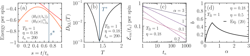
Figure 1: (a) Energy expectation values, $\langle H_{\rm S}(t/{t_{\rm a}})\rangle_{t}$ and $\langle H_{\rm S}(s)\rangle_{s,T_{\rm B}}^{\rm eq}$, per spin of the time-dependent state $\rho_{\rm S}(t)$ and the instantaneous thermal equilibrium state $\rho_{\rm S}^{\rm eq}(s,T_{\rm B})$, respectively, as functions of the rescaled time $s$ for $t_{\mathrm{a}}=200$ and $\eta=0.18$ at $T_{\rm B}=1$. We fixed $\alpha=1$. The dashed line and the solid vertical line indicate $\frac{1}{N}\langle H_{\rm I}\rangle_{t_{a}}t/t_{a}$ and $s^{*}\equiv T_{\rm B}/T^{\ast}$, respectively, where $T^{\ast}$ is determined by the minimization of the Kullback–Leibler (KL) divergence. (b) KL divergence $D_{\rm KL}(T)$ between the final state after QA and the Gibbs state of $H_{\rm I}$ with temperature $T$. See the main text for a detailed definition. (c) Excess energy $\mathcal{E}_{\mathrm{exc}}$ per spin from the thermal expectation value after QA as a function of $t_{\mathrm{a}}$ for various $\alpha$. Lines indicate the best power-law fits $\mathcal{E}_{\rm exc}=at_{a}^{-b}$ to the data for $t_{\mathrm{a}}>100$ with the fitting parameters $a$ and $b$. (d) Exponent $b$ as a function of $\alpha$. The numerical results (symbols) are compared to the theoretical prediction shown by the solid line. The parameters used in the numerical simulations are $\omega_{c}=5$, $\tau_{c}=10$, $\Delta t=0.05$ and $N\to\infty$. The bond dimensions are up to 128.

The key idea of our method is to represent the part of $\exp\mathcal{S}_{\mathrm{infl}}$ associated with a site $j$ in terms of a matrix product state (MPS) as follows:

$$\exp\Biggl{(}\sum_{l>m}^{|t_{l}-t_{m}|<\tau_{c}}\kappa_{l,m}\sigma_{j}^{(l)}\sigma_{j}^{(m)}\Biggr{)}$$

$$\approx\sum_{\{\mu_{j,l}\}}^{\chi_{t}}\phi^{(j,0)S^{(0)}_{j}}_{\mu_{j,0}}\phi^{(j,1)S^{(1)}_{j}}_{\mu_{j,0},\mu_{j,1}}\phi^{(j,2)S^{(2)}_{j}}_{\mu_{j,1},\mu_{j,2}}\cdots\phi^{(j,M)S^{(M)}_{j}}_{\mu_{j,M-1}},$$ (14)

where $S_{j}^{(l)}\equiv(\sigma_{j}^{(l)},~{}\sigma_{j}^{(2M+1-l)})$ denotes the composite variable and $\chi_{t}$ is the bond dimension which controls the precision of the approximation in this MPS representation. The tensors $\phi^{(j,l)}$ are given by recursive application of the singular value decomposition [48, 40]. Using Eq. (14) in Eq. (8), we obtain a tensor network representation for the RDM:

$$\bra{\boldsymbol{\sigma}^{(M)}}\rho_{\mathrm{S}}(t)\ket{\boldsymbol{\sigma}^{(M+1)}}$$ (15)

$$\approx\sum_{\{S_{j}^{(l)},\mu_{j,l}\}_{l\neq M}}e^{i\mathcal{S}_{\mathrm{0}}}\prod_{j=1}^{N}\phi^{(j,0)S^{(0)}}_{\mu_{j,0}}\Bigl{[}\prod_{l=1}^{M-1}\phi_{\mu_{j,l-1},\mu_{j,l}}^{(j,l)S_{j}^{(l)}}\Bigr{]}\phi^{(j,M)S^{(M)}_{j}}_{\mu_{j,M-1}}.$$

Having obtained this tensor network representation, the iTEBD algorithm can be applied to implement the sum with respect to $\{S_{j}^{(l)},\mu_{j,l}\}_{l\neq M}$ and compute local quantities, taking $N\to\infty$ and using the translational invariance in space [42].

Phenomenological theory.— Let us assume a finite bath temperature $T_{\rm B}>0$. In the limiting case of $t_{\rm a}\to\infty$, QA in this thermal environment leads to the quasistatic and isothermal process. Accordingly, the final state of the spin system is described by $\rho^{\rm eq}_{\rm S}(1,T_{\rm B})=\rho_{\rm I}^{\rm eq}(T_{\rm B})$. When $t_{\rm a}$ is finite, the spin system approximately maintains thermal equilibrium as long as the relaxation time of the spin system is shorter than the annealing time scale. However, in the case of $[H_{\rm S}(1),H_{\rm SB}]=0$, it is known that the relaxation time grows infinitely with $s\to 1$. Therefore the quasistatic and isothermal evolution must fail before QA ends, and the spin state is expected to be frozen at a time $t^{\ast}=s^{\ast}t_{\rm a}$ [38, 15]. We refer to $t^{\ast}$ or $s^{\ast}$ as the freezing time. To develop a scaling theory for the freezing time, we employ the quasistatic-freezing approximation as follows. The quasistatic-freezing approximation assumes that the spin state is frozen when the changing rate with $t$ of the instantaneous relaxation time of the spin system exceeds unity. Writing the instantaneous relaxation time at $s=t/t_{\rm a}$ as $\tau_{\mathrm{rel}}(s)$, the freezing time is then determined by

$$\dot{\tau}_{\mathrm{rel}}(s^{*})=1,$$ (16)

where the dot denotes differentiation by $t$. $\tau_{\mathrm{rel}}(s)$ is now estimated from the transition rate $\gamma(s)$. Using Fermi’s golden rule, the latter is given, up to an $s$-independent factor, as

$$\gamma_{l,m}(s)\propto\eta|\bra{\psi_{l}(s)}\sum_{i}\hat{\sigma}^{z}_{i}\ket{\psi_{m}(s)}|^{2}$$ (17)

where $\ket{\psi_{l}(s)}$ and $\ket{\psi_{m}(s)}$ are the $l$-th and $m$-th eigenstates of $H_{\mathrm{S}}(s)$, respectively. When $s$ is close to 1, $|\psi_{l}(s)\rangle$ is written within the first order of $A(s)$ as $|\psi_{l}(s)\rangle\approx|\psi_{l}(1)\rangle+A(s)\sum_{m\neq l}[\langle\psi_{l}(1)|H_{\rm TF}|\psi_{m}(1)\rangle/(E_{l}-E_{m})]|\psi_{m}(1)\rangle$, where $E_{m}$ denotes an eigenenergy of $B(s)H_{\rm I}$. Using this and noting that $\sum_{i}\hat{\sigma}^{z}_{i}$ is diagonal with the basis $\{|\psi_{m}(1)\rangle\}$, one finds that Eq. (17) is proportinal to $\eta A(s)^{2}$. Therefore, the scaling of relaxation time is obtained as

$$\tau_{\mathrm{rel}}(s)\approx\gamma_{l,m}(s)^{-1}\sim\eta^{-1}A(s)^{-2}\sim\eta^{-1}(1-s)^{-2\alpha}.$$ (18)

Using this in Eq. (16), the scaling relation of $s^{\ast}$ is obtained as follows:

$$(1-s^{\ast})\sim(\eta t_{\mathrm{a}})^{-1/(2\alpha+1)}.$$ (19)

Now, the quasistatic-freezing approximation implies that the RDM after the freezing time is approximately replaced by that of the instantaneous thermal equilibrium at $s=s^{\ast}$, namely, $\rho_{\rm S}(t)\approx\rho_{\rm S}^{\rm eq}(s^{\ast},T_{\rm B})$ for $t>s^{\ast}t_{\rm a}$. Moreover, $\rho_{\rm S}^{\rm eq}(s^{\ast},T_{\rm B})$ can be approximated by the Gibbs state $\rho_{\rm S}^{\rm Gibbs}\equiv e^{-H_{\rm S}(s^{\ast})/T_{\rm B}}/{\rm Tr}[e^{-H_{\rm S}(s^{\ast})/T_{\rm B}}]$ for sufficiently weak $\eta$, and the latter is approximated as $\rho_{\rm S}^{\rm Gibbs}\approx\rho_{\rm I}^{\rm eq}(T_{\rm B}/{B(s^{\ast})})+O(A(s^{\ast}))$ near $s^{\ast}=1$. Therefore, neglecting the $O(A(s^{\ast})^{2})$ and $O(A(s)A(s^{\ast}))$ terms for $\alpha>\frac{1}{2}$, the energy of the spin system for $t>s^{\ast}t_{\rm a}$ is estimated as [49]

$$\langle H_{\rm S}(t/t_{\rm a})\rangle_{t}\approx B(t/t_{\rm a})\langle H_{\rm I}\rangle^{\rm eq}_{{\rm I},T_{\rm B}/{B(s^{\ast})}},$$ (20)

where $\langle\cdot\rangle_{t}$ and $\langle\cdot\rangle^{\rm eq}_{{\rm I},T}$ represent the expectation values with respect to $\rho_{\rm S}(t)$ and $\rho_{\rm I}^{\rm eq}(T)$, respectively. Therefore, the energy of the spin system approaches the thermal expectation value of $H_{\rm I}$ at the temperature $T_{\rm B}/{B(s^{\ast})}$ as $s\to 1$. For general $\alpha>0$, expanding $\rho_{\rm S}^{\rm Gibbs}$ in series of $(1-s^{\ast})$ and $(1-s^{\ast})^{\alpha}$ perturbatively, one obtains $\langle H_{\rm S}(1)\rangle_{t_{\rm a}}\approx\langle H_{\rm S}(1)\rangle^{\rm eq}_{{\rm I},T_{\rm B}}+c_{1}(1-s^{\ast})+c_{2}(1-s^{\ast})^{2\alpha}$ [49], where $c_{1}$ and $c_{2}$ are coefficients independent of $s^{\ast}$. Keeping the leading term and applying Eq. (19), the excess energy of the final state is obtained as

$$\mathcal{E}_{\rm exc}\equiv\langle H_{\rm S}(1)\rangle_{t_{\rm a}}-\langle H_{\rm S}(1)\rangle^{\rm eq}_{{\rm I},T_{\rm B}}\sim(\eta~{}t_{\mathrm{a}})^{-b},$$ (21)

with

$$b=\min\{1,2\alpha\}/({2}\alpha+1).$$ (22)

Note that the excess energy decays the fastest when $\alpha=\frac{1}{2}$. Equations (21) and (22) are valid for DQIC in any dimension, any lattice and non-Ohmic spectral densities as well.

Numerical results.— Figure 1(a) shows the energy expectation value per site of the time-dependent state during QA and that of the instantaneous thermal equilibrium as functions of the rescaled time $s$. After the initial relaxation, the system maintains thermal equilibrium until a certain time $s^{\ast}$, when the quasistatic and isotheral evolution fails and the energy deviates upwards from that of the instantaneous equilibrium state. This behavior is perfectly consistent with the quasistatic-freezing picture mentioned above. To evaluate the freezing time $s^{\ast}$ and identify the final energy $\langle H_{\rm I}\rangle_{{t_{\rm a}}}$, we focus on the Kullback-Leibler (KL) divergence $D_{\rm KL}$ of the final state and the Boltzmann distribution of $H_{\rm I}$ as a measure of the distance between the two. Because this quantity is not accessible for the RDMs of the entire spin system when using our method, we instead consider the RDMs of eight spins given by $\rho_{8}\equiv{\rm Tr}_{\bar{8}}\rho_{\rm S}({t_{\rm a}})$ and $\rho_{8}^{\rm eq}(T)\equiv{\rm Tr}_{\bar{8}}\rho_{\rm I}^{\rm eq}(T)$ to define $D_{\rm KL}(T)\equiv{\rm Tr}_{8}[\rho_{8}(\log\rho_{8}-\log\rho_{8}^{\rm eq}(T))]$, where ${\rm Tr}_{8}$ and ${\rm Tr}_{\bar{8}}$ denote the trace with respect to the eight adjacent spins and the other spins, respectively. We show $D_{\rm KL}(T)$ in Fig. 1(b). $D_{\rm KL}(T)$ has a sharp minimum at a certain $T$ labeled $T^{\ast}$. This implies that the RDM after QA is approximated by the Gibbs state of $H_{\rm I}$ with the temperature $T^{\ast}$. In addition, as shown in Fig. 1(a), the curve of $\langle H_{\rm S}(t/{t_{\rm a}})\rangle_{t}$ is indistinguishable from the line of $s\langle H_{\rm I}\rangle_{{\rm I},T^{\ast}}$ near $s=1$. Assuming $T^{\ast}=T/s^{\ast}$, this result implies Eq. (20) and that $s^{\ast}$ determined by $T/T^{\ast}$ is consistent with the freezing time when the quasistatic evolution fails (see the vertical line in Fig. 1(a)). Figure 1(c) shows the excess energy as a function of the annealing time $t_{\rm a}$ for $\eta=0.18$ and $T_{\rm B}=1$. It can be seen that the excess energy decays as a power law for large $t_{\rm a}$ with an exponent denoted by $b$ that depends on $\alpha$. Figure 1(d) shows the $\alpha$ dependence of the exponent $b$. There is excellent agreement between the numerical results and the theoretical prediction.

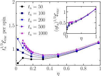
Figure 2: Excess energy per spin after QA scaled by $t_{\mathrm{a}}^{-1/3}$ as a function of $\eta$ for $T_{\rm B}=1$, $\alpha=1$, and various ${t_{\rm a}}$ ranging from 50 to 1000. With increasing $t_{\rm a}$, the data collapse into a single nonmonotonic curve, which implies $\mathcal{E}_{\rm exc}\sim t_{\rm a}^{-1/3}$ for large $t_{\rm a}$. The inset shows the data rescaled by $(\eta t_{\mathrm{a}})^{-1/3}$. The constancy of the data with large $t_{\rm a}$ near $\eta=0$ corresponds to Eq. (21). The parameters in the numerical simulations are the same as those in Fig. 1.

Figure 2 shows the $\eta$-dependence of $\mathcal{E}_{\rm exc}$ scaled by $t_{\mathrm{a}}^{1/3}$ for $T_{\rm B}=1$, $\alpha=1$, and various ${t_{\rm a}}$. It can be seen that $\mathcal{E}_{\rm exc}$ is nonmonotonic with respect to $\eta$. The decreasing behavior of $\mathcal{E}_{\rm exc}$ with increasing $\eta$ in the weak coupling regime is consistent with Eq. (21), while its increasing behavior in the strong-coupling regime ($\eta\gtrsim 0.4$) is not described by the phenomenological theory mentioned above. This failure of the theory arises from the perturbative argument used for the relaxation time in Eq. (17). The existence of the optimal strength in the system-bath coupling to reduce $\mathcal{E_{\rm exc}}$ is first revealed by our numerical method based on a non-perturbative formulation. Note that the scaling of $\mathcal{E}_{\rm exc}$ by $t_{\rm a}$ is valid even in the case of strong-coupling.

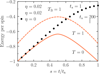
Figure 3: Energy expectation values per spin as functions of the rescaled time $s$. The solid and dashed lines show the energies per spin of the instantaneous equilibrium states of the closed system at $T=0$ and $T=1$ , respectively. The filled symbols show the energy of the time-dependent state for $t_{\rm a}=1$ of the closed system ($\eta=0$). The empty symbols denote energies of the time-dependent states of the dissipative system with $\eta=0.02$ and $T_{\rm B}=1$ for $t_{\rm a}=1$ and $t_{\rm a}=200$. We fixed $\alpha=1$. The parameters in the numerical simulations are the same as those in Fig. 1.

So far, we have focused on slow QA in a thermal environment with a finite temperature and have discussed consequences of freezing near the end of annealing. Here, we comment on two situations where the dynamics is governed by a quantum phase transition (QPT) at zero temperature, assuming the absence of a thermal phase transition at finite temperature. The first is the case of weak-coupling and short-annealing-time. When the system-bath coupling is sufficiently weak, i.e. $\eta\ll 1$, QA drives the spin system in the same way as a closed system as long as ${t_{\rm a}}$ is not large, as demonstrated by the proximity of filled and empty circles in Fig. 3. In this case, the QPT governs the dynamics, and gives rise to the Kibble–Zurek scaling (KZS) [50, 51, 52] of the residual energy to the ground state after QA. For larger ${t_{\rm a}}$, the system is thermalized and the QPT no longer affect the dynamics as shown by the overlap of squares with the dashed line in Fig. 3. The crossover from the KZS regime to the large $t_{\rm a}$ regime is accompanied by a non-monotonic change in the residual energy when $T_{\rm B}$ is sufficiently high [53]. The second is the case of medium-coupling and low-temperature, where the dynamics is governed by a QPT of the dissipative system at $T_{\rm B}=0$. In this case, KZS with a modified exponent [40] is observed. When the temperature is not low and/or ${t_{\rm a}}$ is much larger, however, the spin system is not influenced by a QPT and the quasistatic-freezing picture is valid because the time scale of QA is beyond the characteristic time in the quantum critical region [53]. A recent experimental study suggests that systems realized in the D-Wave device should be in a situation with a medium $\eta$ and a low $T_{\rm B}$ [36]. Therefore, if one performs experiments with still longer ${t_{\rm a}}$ or higher $T_{\rm B}$, the scaling of the excess energy given by Eqs.  (21) and (22) should be observed.

Summary.— We studied QA in a thermal environment. The simulation using the non-Markovian iTEBD not only confirmed the phenomenological theory for weak system-bath coupling but revealed a nontrivial behavior of the excess energy after QA in the regime beyond weak coupling. The findings presented here will be beneficial in designing and evaluating QA devices. Other system-bath couplings, non-Ohmic baths, and other driven DQICs are open to numerical study with the non-Markovian iTEBD method.

The authors acknowledge H. Nishimori and Y. Susa for valuable discussions, and Y. Bando M. Ohzeki, F. J. Gómez-Ruiz, A. del Campo, and D. A. Lidar for collaboration on a related experimental project.

References

- Johnson et al. [2011] M. W. Johnson, M. H. Amin, S. Gildert, T. Lanting, F. Hamze, N. Dickson, R. Harris, A. J. Berkley, J. Johansson, P. Bunyk, E. M. Chapple, C. Enderud, J. P. Hilton, K. Karimi, E. Ladizinsky, N. Ladizinsky, T. Oh, I. Perminov, C. Rich, M. C. Thom, E. Tolkacheva, C. J. Truncik, S. Uchaikin, J. Wang, B. Wilson, and G. Rose, Nature 473, 194 (2011).
- Boixo et al. [2014] S. Boixo, T. F. Rønnow, S. V. Isakov, Z. Wang, D. Wecker, D. A. Lidar, J. M. Martinis, and M. Troyer, Nature Physics 10, 218 (2014).
- Denchev et al. [2016] V. S. Denchev, S. Boixo, S. V. Isakov, N. Ding, R. Babbush, V. Smelyanskiy, J. Martinis, and H. Neven, Phys. Rev. X 6, 031015 (2016).
- Albash and Lidar [2018a] T. Albash and D. A. Lidar, Phys. Rev. X 8, 031016 (2018a).
- King et al. [2018] A. D. King, J. Carrasquilla, J. Raymond, I. Ozfidan, E. Andriyash, A. Berkley, M. Reis, T. Lanting, R. Harris, F. Altomare, K. Boothby, P. I. Bunyk, C. Enderud, A. Fréchette, E. Hoskinson, N. Ladizinsky, T. Oh, G. Poulin-Lamarre, C. Rich, Y. Sato, A. Y. Smirnov, L. J. Swenson, M. H. Volkmann, J. Whittaker, J. Yao, E. Ladizinsky, M. W. Johnson, J. Hilton, and M. H. Amin, Nature 560, 456 (2018).
- Harris et al. [2018] R. Harris, Y. Sato, A. J. Berkley, M. Reis, F. Altomare, M. H. Amin, K. Boothby, P. Bunyk, C. Deng, C. Enderud, S. Huang, E. Hoskinson, M. W. Johnson, E. Ladizinsky, N. Ladizinsky, T. Lanting, R. Li, T. Medina, R. Molavi, R. Neufeld, T. Oh, I. Pavlov, I. Perminov, G. Poulin-Lamarre, C. Rich, A. Smirnov, L. Swenson, N. Tsai, M. Volkmann, J. Whittaker, and J. Yao, Science 361, 162 (2018).
- King et al. [2019] A. D. King, J. Raymond, T. Lanting, S. V. Isakov, M. Mohseni, G. Poulin-Lamarre, S. Ejtemaee, W. Bernoudy, I. Ozfidan, A. Y. Smirnov, M. Reis, F. Altomare, M. Babcock, C. Baron, A. J. Berkley, K. Boothby, P. I. Bunyk, H. Christiani, C. Enderud, B. Evert, R. Harris, E. Hoskinson, S. Huang, K. Jooya, A. Khodabandelou, N. Ladizinsky, R. Li, P. A. Lott, A. J. R. MacDonald, D. Marsden, G. Marsden, T. Medina, R. Molavi, R. Neufeld, M. Norouzpour, T. Oh, I. Pavlov, I. Perminov, T. Prescott, C. Rich, Y. Sato, B. Sheldan, G. Sterling, L. J. Swenson, N. Tsai, M. H. Volkmann, J. D. Whittaker, W. Wilkinson, J. Yao, H. Neven, J. P. Hilton, E. Ladizinsky, M. W. Johnson, and M. H. Amin, “Scaling advantage in quantum simulation of geometrically frustrated magnets,” (2019), arXiv:1911.03446 [quant-ph] .
- Ushijima-Mwesigwa et al. [2017] H. Ushijima-Mwesigwa, C. F. A. Negre, and S. M. Mniszewski, in Proceedings of the Second International Workshop on Post Moores Era Supercomputing, PMES’17 (Association for Computing Machinery, New York, NY, USA, 2017) pp. 22–29, event-place: Denver, CO, USA.
- Teplukhin et al. [2020] A. Teplukhin, B. K. Kendrick, S. Tretiak, and P. A. Dub, Scientific Reports 10, 20753 (2020).
- Boixo et al. [2013] S. Boixo, T. Albash, F. M. Spedalieri, N. Chancellor, and D. A. Lidar, Nature Communications 4, 2067 (2013).
- Marshall et al. [2017] J. Marshall, E. G. Rieffel, and I. Hen, Phys. Rev. Applied 8, 064025 (2017).
- Sarandy and Lidar [2005] M. S. Sarandy and D. A. Lidar, Phys. Rev. Lett. 95, 250503 (2005).
- Amin et al. [2008] M. H. S. Amin, P. J. Love, and C. J. S. Truncik, Phys. Rev. Lett. 100, 060503 (2008).
- Dickson et al. [2013] N. G. Dickson, M. W. Johnson, M. H. Amin, R. Harris, F. Altomare, A. J. Berkley, P. Bunyk, J. Cai, E. M. Chapple, P. Chavez, F. Cioata, T. Cirip, P. deBuen, M. Drew-Brook, C. Enderud, S. Gildert, F. Hamze, J. P. Hilton, E. Hoskinson, K. Karimi, E. Ladizinsky, N. Ladizinsky, T. Lanting, T. Mahon, R. Neufeld, T. Oh, I. Perminov, C. Petroff, A. Przybysz, C. Rich, P. Spear, A. Tcaciuc, M. C. Thom, E. Tolkacheva, S. Uchaikin, J. Wang, A. B. Wilson, Z. Merali, and G. Rose, Nature Communications 4, 1903 (2013).
- Amin [2015] M. H. Amin, Phys. Rev. A 92, 052323 (2015).
- Arceci et al. [2017] L. Arceci, S. Barbarino, R. Fazio, and G. E. Santoro, Phys. Rev. B 96, 054301 (2017).
- Smelyanskiy et al. [2017] V. N. Smelyanskiy, D. Venturelli, A. Perdomo-Ortiz, S. Knysh, and M. I. Dykman, Phys. Rev. Lett. 118, 066802 (2017).
- Smirnov and Amin [2018] A. Y. Smirnov and M. H. Amin, New Journal of Physics 20, 103037 (2018).
- Kadowaki and Nishimori [1998] T. Kadowaki and H. Nishimori, Phys. Rev. E 58, 5355 (1998).
- Finnila et al. [1994] A. Finnila, M. Gomez, C. Sebenik, C. Stenson, and J. Doll, Chemical Physics Letters 219, 343 (1994).
- Das and Chakrabarti [2005] A. Das and B. K. Chakrabarti, eds., Quantum annealing and related optimization methods (Springer, Berlin, Heidelberg, 2005) lecture Notes in Physics, Vol. 679.
- Das and Chakrabarti [2008] A. Das and B. K. Chakrabarti, Rev. Mod. Phys. 80, 1061 (2008).
- Albash and Lidar [2018b] T. Albash and D. A. Lidar, Rev. Mod. Phys. 90, 015002 (2018b).
- Hauke et al. [2020] P. Hauke, H. G. Katzgraber, W. Lechner, H. Nishimori, and W. D. Oliver, Reports on Progress in Physics 83, 054401 (2020).
- Farhi et al. [2001] E. Farhi, J. Goldstone, S. Gutmann, J. Lapan, A. Lundgren, and D. Preda, Science 292, 472 (2001).
- Patanè et al. [2008] D. Patanè, A. Silva, L. Amico, R. Fazio, and G. E. Santoro, Phys. Rev. Lett. 101, 175701 (2008).
- Patanè et al. [2009] D. Patanè, L. Amico, A. Silva, R. Fazio, and G. E. Santoro, Phys. Rev. B 80, 024302 (2009).
- Yin et al. [2014] S. Yin, P. Mai, and F. Zhong, Phys. Rev. B 89, 094108 (2014).
- Hwang et al. [2015] M.-J. Hwang, R. Puebla, and M. B. Plenio, Phys. Rev. Lett. 115, 180404 (2015).
- Nalbach et al. [2015] P. Nalbach, S. Vishveshwara, and A. A. Clerk, Phys. Rev. B 92, 014306 (2015).
- Dutta et al. [2016] A. Dutta, A. Rahmani, and A. del Campo, Phys. Rev. Lett. 117, 080402 (2016).
- Keck et al. [2017] M. Keck, S. Montangero, G. E. Santoro, R. Fazio, and D. Rossini, New Journal of Physics 19, 113029 (2017).
- Weinberg et al. [2020] P. Weinberg, M. Tylutki, J. M. Rönkkö, J. Westerholm, J. A. Åström, P. Manninen, P. Törmä, and A. W. Sandvik, Phys. Rev. Lett. 124, 090502 (2020).
- Puebla et al. [2020] R. Puebla, A. Smirne, S. F. Huelga, and M. B. Plenio, Phys. Rev. Lett. 124, 230602 (2020).
- Rossini and Vicari [2020] D. Rossini and E. Vicari, Phys. Rev. Research 2, 023211 (2020).
- Bando et al. [2020] Y. Bando, Y. Susa, H. Oshiyama, N. Shibata, M. Ohzeki, F. J. Gómez-Ruiz, D. A. Lidar, S. Suzuki, A. del Campo, and H. Nishimori, Phys. Rev. Research 2, 033369 (2020).
- Bandyopadhyay et al. [2020] S. Bandyopadhyay, S. Bhattacharjee, and A. Dutta, Phys. Rev. B 101, 104307 (2020).
- Albash et al. [2012] T. Albash, S. Boixo, D. A. Lidar, and P. Zanardi, New Journal of Physics 14, 123016 (2012).
- Marshall et al. [2019] J. Marshall, D. Venturelli, I. Hen, and E. G. Rieffel, Phys. Rev. Applied 11, 044083 (2019).
- Oshiyama et al. [2020] H. Oshiyama, N. Shibata, and S. Suzuki, J. Phys. Soc. Japan 89, 1 (2020).
- Makri [1992] N. Makri, Chemical Physics Letters 193, 435 (1992).
- Orús and Vidal [2008] R. Orús and G. Vidal, Phys. Rev. B 78, 155117 (2008).
- Caldeira and Leggett [1983] A. O. Caldeira and A. J. Leggett, Ann. Phys. (N. Y). 149, 374 (1983).
- Leggett et al. [1987] A. J. Leggett, S. Chakravarty, A. T. Dorsey, M. P. A. Fisher, A. Garg, and W. Zwerger, Rev. Mod. Phys. 59, 1 (1987).
- Trotter [1959] H. F. Trotter, Proceedings of the American Mathematical Society 10, 545 (1959).
- Suzuki [1976] M. Suzuki, Progress of Theoretical Physics 56, 1454 (1976).
- Makarov and Makri [1994] D. E. Makarov and N. Makri, Chemical Physics Letters 221, 482 (1994).
- Suzuki et al. [2019] S. Suzuki, H. Oshiyama, and N. Shibata, J. Phys. Soc. Japan 88, 061003 (2019), https://doi.org/10.7566/JPSJ.88.061003 .
- [49] Note here that the terms proportional to vanish in , since has no diagonal elements in the eigenbasis of .
- Kibble [1976] T. W. B. Kibble, Journal of Physics A: Mathematical and General 9, 1387 (1976).
- Zurek [1985] W. H. Zurek, Nature 317, 505 (1985).
- Dziarmaga [2005] J. Dziarmaga, Phys. Rev. Lett. 95, 245701 (2005).
- [53] See Supplementary Materials.