First-Passage Time Statistics on Surfaces of General Shape:
Surface PDE Solvers using Generalized Moving Least Squares (GMLS)

We develop numerical methods for computing statistics of stochastic processes on surfaces of general shape with drift-diffusion dynamics $d\mathbf{X}_{t}=a(\mathbf{X}_{t})dt+\mathbf{b}(\mathbf{X}_{t})d\mathbf{W}_{t}$. We formulate descriptions of Brownian motion and general drift-diffusion processes on surfaces. We consider statistics of the form $u(\mathbf{x})=\mathbb{E}^{\mathbf{x}}\left[\int_{0}^{\tau}g(\mathbf{X}_{t})dt\right]+\mathbb{E}^{\mathbf{x}}\left[f(\mathbf{X}_{\tau})\right]$ for a domain $\Omega$ and the exit stopping time $\tau=\inf_{t}\{t>0\;|\;\mathbf{X}_{t}\not\in\Omega\}$, where $f,g$ are general smooth functions. For computing these statistics, we develop high-order Generalized Moving Least Squares (GMLS) solvers for associated surface PDE boundary-value problems based on Backward-Kolmogorov equations. We focus particularly on the mean First Passage Times (FPTs) given by the case $f=0,\,g=1$ where $u(\mathbf{x})=\mathbb{E}^{\mathbf{x}}\left[\tau\right]$. We perform studies for a variety of shapes showing our methods converge with high-order accuracy both in capturing the geometry and the surface PDE solutions. We then perform studies showing how statistics are influenced by the surface geometry, drift dynamics, and spatially dependent diffusivities.

Introduction

Path-related statistics of stochastic processes, such as the mean First Passage Times (FPTs) [3, 20, 17], arise in many fields, including in biology [46, 54, 49, 55, 43, 73], physics [57, 48, 8, 66, 13, 56], engineering [60, 51, 26], finance [45, 1, 30, 39], and machine learning [27, 70]. Many problems involve stochastic processes within manifolds where significant roles are played by geometric and topological contributions [52, 57, 48, 44, 61, 73]. We consider Ito processes $\mathbf{X}_{t}$ with the drift-diffusion dynamics $d\mathbf{X}_{t}=a(\mathbf{X}_{t})dt+\mathbf{b}(\mathbf{X}_{t})d\mathbf{W}_{t}$, [17, 6]. We formulate descriptions of Brownian motion and general drift-diffusion processes on surfaces. While in principle statistics can be estimated by using stochastic numerical methods to sample trajectories $\{\mathbf{X}_{t}\}_{0\leq t\leq T}$, it can be computationally expensive to reduce statistical sampling errors sufficiently. Further challenges also arise when the process has multiple dynamical times-scales resulting in stiffness, or when trying to estimate statistics at many locations on the surface [11, 6, 13, 49].

In practice, for making predictions of observations and measurements, it is often enough to consider the class of statistics of the form $u(\mathbf{x})=\mathbb{E}^{\mathbf{x}}\left[\int_{0}^{\tau}g(\mathbf{X}_{t})dt\right]+\mathbb{E}^{\mathbf{x}}\left[f(\mathbf{X}_{\tau})\right]$. For the stochastic process, the $\mathbf{X}_{0}=\mathbf{x}\in\Omega$ within an open domain $\Omega$ and the exit stopping time is $\tau=\inf_{t}\{t>0\;|\;\mathbf{X}_{t}\not\in\Omega\}$. The choice of $g$ can be used to obtain information about the states $\mathbf{x}\in\Omega$ realized by the stochastic trajectories. The choice of $f$ can be used to obtain information about where the stochastic trajectories encounter the boundary $\partial\Omega$. The Dynkin formula and Backward-Kolmogorov equations provide connections between these statistics and a collection of elliptic Partial Differential Equations (PDEs) with boundary values problems of the form $\mathcal{L}u=-g,\,\,\mathbf{x}\in\Omega,\,\,u=f,\,\,\mathbf{x}\in\partial\Omega$, [17].

We develop numerical methods for solving these PDEs on manifolds of general shape based on meshless methods. Meshless methods can be characterized broadly by their underlying discretizations. This includes Radial Basis Functions (RBF), Generalized Finite Differences (GFD), Moving Least Squares (MLS), and Reproducing Kernel Particle Methods (RKPM), [4, 21, 5, 12, 9, 10]. While most meshfree approaches are for solutions of PDEs in euclidean spaces $\mathbb{R}^{d}$ with $d=1,2,3$, recent work has focused on the manifold setting, including [33, 40, 69, 64, 68, 42, 65, 37, 38]. This includes methods for stablizing RBFs [32, 35, 28], semi-lagrangian methods [64], approaches avoiding use of surface coordinates [53, 63], and methods that make use of the embedding space [37, 62, 29]. This also includes methods using least-squares methods [41, 71, 72] and generalized finite difference approaches [25, 59].

For surfaces of general shape, we develop high-order numerical methods for computing statistics using Generalized Moving Least Squares (GMLS) approximations [36, 23]. Our approaches provide meshless methods for solving PDEs on surfaces related to [41, 71, 72, 25, 59]. We focus here primarily on mean First Passage Times (FPTs), which are given by the special case $f=0,\,g=1$ with $u(\mathbf{x})=\mathbb{E}^{\mathbf{x}}\left[\tau\right]$. Our methods also can be readily extended for the cases with more general $f,g$. We perform studies for a variety of shapes to investigate how the methods converge. We show our methods can accurately capture both the surface geometry and the action of the surface differential operators. We then perform convergence studies which show our methods have a high-order accuracy in approximating solutions of the surface PDEs. We show how our methods can be used to study how statistics are affected by the surface geometry, drift dynamics, and spatially dependent diffusivities. We also discuss how the methods can be extended for computing more general path-dependent statistics for stochastic processes on surfaces.

1 First-Passage Times and Path-Dependent Statistics on Surfaces

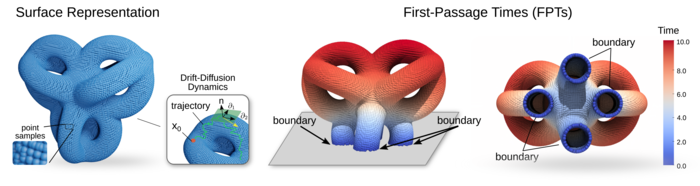
Figure 1: Path-Dependent Statistics and Geometry. (left) We develop meshless numerical methods for solving surface PDEs associated with path-dependent statistics of general drift-diffusion stochastic processes on surfaces of the form $d\mathbf{X}_{t}=\mathbf{a}(\mathbf{X}_{t})dt+\mathbf{b}(\mathbf{X}_{t})d\mathbf{W}_{t}$. Statistics include the mean First Passage Times (FPTs) where the geometry and topology may play significant roles. (middle) In FPTs, the process starts at $\mathbf{X}(0)=\mathbf{x}_{0}$ and the average time is computed for arriving at the boundary created by slicing the surface at $z=0$. The surface geometry is represented by a collection of point samples. (right) The surface colors indicate the value of the FPT to reach the boundary when starting at a location on the surface. The results shown are for surface diffusion with $\mathbf{a}(\mathbf{x})=0$ and $\mathbf{b}(\mathbf{x})=I$.

The mean First-Passage Time (FPT) is defined as

$$u(\mathbf{x}_{0})=\mathbb{E}^{\small X(0)=\mathbf{x}_{0}}\left[\tau\right],\;\;\mbox{where }\tau=\inf\{t>0\,|\,\mathbf{X}_{t}\not\in\Omega\}.$$ (1)

This gives the time $\tau$ for a particle starting at location $X(0)=\mathbf{x}_{0}\in\Omega$ to reach the boundary of the domain $\partial\Omega$. We denote by $u(\mathbf{x}_{0})$ the average value of this passage time. In Figure 1, we show the case of a curved surface with boundary defined by a cut-plane at $z=0$. The color at $\mathbf{x}$ indicates $u(\mathbf{x})$ for the mean first passage time for a diffusion on the surface starting at $\mathbf{x}$ to reach the boundary at $z=0$, see Figure 1.

We consider the general drift-diffusion dynamics constrained to a surface $\mathcal{M}$ governed by the Stochastic Differential Equations (SDEs)

$$d\mathbf{X}_{t}=\mathbf{a}(\mathbf{X}_{t})dt+\mathbf{b}(\mathbf{X}_{t})d\mathbf{W}_{t},\hskip 14.22636pt\mbox{subject to }\mathbf{X}_{t}\in\mathcal{M}.$$ (2)

The $\mathbf{a}(\mathbf{x})$ term models the local drift in the dynamics and the $\mathbf{b}(\mathbf{x})$ the local diffusivity. The $d\mathbf{W}_{t}$ denotes increments of the Weiner process. Throughout, we interpret our SDEs in terms of Ito stochastic processes [17, 6].

While in principle stochastic simulations can be used to sample trajectories for Monte-Carlo estimates of statistics, in practice this can be expensive. This arises from the need to reduce sufficiently the statistical sampling errors, which can become particularly expensive when computing statistics for many initial starting locations. Further challenges arise when there are disparate time-scales in the dynamics resulting in numerical stiffness or in rare-events that result in slow decay of the statistical errors [15, 49]. We develop alternative approaches using Dynkin’s formula and the Backward-Kolmogorov equations [17]. This relates the FPTs, and other path-dependent statistics, to elliptic PDE boundary value problems. We develop numerical methods for solving these surface PDEs.

For the stochastic process $\mathbf{X}_{t}$, we consider path-dependent statistics $u$ of the form

$$u(\mathbf{x})=\mathbb{E}^{\mathbf{x}}\left[\int_{0}^{\tau}g(\mathbf{X}_{t})dt\right]+\mathbb{E}^{\mathbf{x}}\left[f(\mathbf{X}_{\tau})\right].$$ (3)

The $g(\mathbf{x})$ allows us to assign a value to individual trajectories based on the locations they traverse inside the domain $\mathbf{x}\in\Omega$. The $f(\mathbf{x})$ allows for assigning a cost for the location where the process hits the boundary $\mathbf{x}\in\partial\Omega$. The Dynkin formula for $q(\mathbf{x})$ is given by [17]

$$\mathbb{E}^{\mathbf{x}}\left[q(\mathbf{X}_{\tau})\right]=q(\mathbf{x})+\mathbb{E}^{\mathbf{x}}\left[\int_{0}^{\tau}\mathcal{L}q(\mathbf{X}_{s})ds\right].$$ (4)

The $\mathcal{L}$ is the Infinitesimal Generator associated with the SDE in equation 2. This can be expressed as the differential operator

$$\mathcal{L}=\mathbf{a}\cdot\frac{\partial}{\partial\mathbf{x}}+\frac{1}{2}\mathbf{b}\mathbf{b}^{T}:\frac{\partial^{2}}{\partial\mathbf{x}^{2}}.$$ (5)

The $\cdot$ denotes the usual dot product with a gradient, and the $:$ denotes the Hadamard element-wise dot product (tensor contraction over indices). We take $q(\mathbf{x})=f(\mathbf{x}),\;\mathbf{x}\in\partial\Omega$ and $\mathcal{L}q(\mathbf{x})=-g(\mathbf{x}),\;\mathbf{x}\in\Omega$. After rearranging terms, we have formally $u(\mathbf{x})=q(\mathbf{x}),\;\mathbf{x}\in\bar{\Omega}$. Using this and equation 5, we can express the statistic $u$ as the solution of a surface elliptic PDE. This gives the PDE boundary-value problem of the form

$$\mathcal{L}u=-g,\,\,\mathbf{x}\in\Omega\,\,\;\;u=f,\,\,\mathbf{x}\in\partial\Omega,$$ (6)

where $\mathcal{L}$ is given in equation 5. We require throughout $f\in C_{0}^{2}(\partial\Omega)$ and $g\in C_{0}^{2}(\Omega)$.

In the case with $f=0$ and $g=-1$, we obtain the mean First-Passage Times (FPTs)

$$u(\mathbf{x})=\mathbb{E}^{\mathbf{x}}\left[\tau\right],\;\;\tau=\inf\{t>0|\mathbf{X}_{t}\neq\Omega\}.$$ (7)

This is the amount of time on average it takes for the drift-diffusion process starting at location $\mathbf{x}$ to hit the boundary of the domain $\partial\Omega$.

To compute these and other path-dependent statistics for stochastic processes constrained to surfaces, we develop solvers for the surface PDEs of equation 6. We show how these methods can be used to investigate the roles played by geometry and the drift-diffusion dynamics in the statistics of equation 3.

1.1 Stochastic Processes and Drift-Diffusion Dynamics on Surfaces

We formulate descriptions for Brownian motion and other more general stochastic processes on surfaces. We express the surface drift-diffusion dynamics using the notation $d\mathbf{X}_{t}=\mathbf{a}dt+\mathbf{b}d\mathbf{W}_{t}.$ The $\mathbf{a}=\mathbf{a}(\mathbf{x})\in\mathbb{R}^{n}$ and $\mathbf{b}=\mathbf{b}(\mathbf{x})\in\mathbb{R}^{n\times m}$. The $\mathbf{X}_{t}\in\mathbb{R}^{n}$ defines the location in terms of the ambient embedding space. In the embedding space we assume the drift $\mathbf{a}$ is in the tangent plane at each point $\mathbf{a}(\mathbf{x})\in T\mathcal{M}_{\mathbf{x}}$ and that the range of the diffusion tensor $\mathbf{b}$ is in the tangent space $\mbox{range}(\mathbf{b})\subset T\mathcal{M}_{\mathbf{x}}$. As a result, the null-space of $\mathbf{b}^{T}$ includes the space of vectors orthogonal to the tangent space $T\mathcal{M}_{\mathbf{x}}$. This has the consequence that $\mathbf{b}\mathbf{b}^{T}$ has a null-space of vectors orthogonal to the tangent space. This also has the range of vectors that are at most spanned by $\mathbf{b}$ in the tangent space, see Figure 1.

In modeling systems, it is often convenient to specify the drift and diffusion using the embedding space representations of $\mathbf{a}$ and $\mathbf{b}$. In numerical methods, and when performing other practical calculations, it is often convenient to express the dynamics using local coordinate charts $\mathbf{q}=(q_{1},q_{2})$ with embedding map $\mathbf{x}=\boldsymbol{\sigma}(q_{1},q_{2})$. It will be convenient to have ways to convert between these types of descriptions. In local coordinate charts, the drift-diffusion dynamics can be expressed as

$$d\mathbf{q}_{t}=\boldsymbol{\alpha}dt+\boldsymbol{\beta}d\tilde{\mathbf{W}}_{t},$$ (8)

where $\boldsymbol{\alpha}(\mathbf{q})\in\mathbb{R}^{2}$ and $\boldsymbol{\beta}(\mathbf{q})\in\mathbb{R}^{2\times\tilde{m}}$ with $\tilde{m}$ the number of noise sources.

These descriptions are connected through the embedding map $\boldsymbol{\sigma}$ given by $\mathbf{X}=\boldsymbol{\sigma}(\mathbf{q})$. We use the Ito Lemma [17] to connect the dynamics in the embedding space with those in the local coordinate chart to obtain

$$d\mathbf{X}_{t} = \left[\alpha^{a}+\frac{1}{2}\Gamma_{ij}^{a}\boldsymbol{\beta}^{i}\boldsymbol{\beta}^{j,T}\right]\boldsymbol{\sigma}_{q^{a}}dt+\boldsymbol{\sigma}_{q^{a}}\boldsymbol{\beta}^{a}d\tilde{\mathbf{W}}_{t}.$$ (9)

The $\Gamma_{ij}^{a}$ are the Christoffel symbols of the surface [19, 7]. We take $\boldsymbol{\beta}^{a}\in\mathbb{R}^{2}$ to be a row vector and $d\tilde{\mathbf{W}}_{t}\in\mathbb{R}^{2}$ to be a column vector. When these combine they give a scalar for each of the coordinate components. We also use the notational conventions that $\partial_{q^{a}}=\partial\boldsymbol{\sigma}/\partial q^{a}=\boldsymbol{\sigma}_{q^{a}}$ and that repeated indices sum. We can use $\{\partial_{q^{a}}\}_{a}$ to represent the dynamics of $\mathbf{X}_{t}$ in the surrounding embedding space. We discuss further details on how to compute these terms from the surface geometry in Appendix A.

We obtain relations between descriptions using the expressions for the dynamics in the embedding space $\mathbb{R}^{3}$ and the dynamics expressed in the coordinates $\mathbf{q}$. These can be summarized as

$$\mathbf{b}\mathbf{b}^{T}=\boldsymbol{\beta}^{a}\boldsymbol{\beta}^{b,T}\partial_{q^{a}}\partial_{q^{b}}^{T}=\boldsymbol{\beta}^{a}\boldsymbol{\beta}^{b,T}\boldsymbol{\sigma}_{q^{a}}\boldsymbol{\sigma}_{q^{b}}^{T},\hskip 17.07182pta^{c}=g^{cb}\langle\mathbf{a},\boldsymbol{\sigma}_{q^{b}}\rangle_{g},\hskip 17.07182pt\alpha^{c}=a^{c}-\frac{1}{2}\Gamma_{ab}^{c}\boldsymbol{\beta}^{a}\boldsymbol{\beta}^{b,T}.$$ (10)

The $\boldsymbol{\beta}^{a}\boldsymbol{\beta}^{b,T}$ is a scalar, since $\boldsymbol{\beta}^{c}$ is a row vector. The $\langle\cdot,\cdot\rangle_{g}$ denotes the inner-product in the embedding space. The $a^{c}$ is useful so that we can represent the vector as $\mathbf{a}=a^{c}\boldsymbol{\sigma}_{q^{c}}$. We still subscript with $g$ even in the embedding space to highlight that this corresponds to the metric inner-product when using a coordinate chart. In practice, this is computed readily if we represent the vectors in the ambient space as the usual Euclidean inner-product between vectors.

While there are many possible choices of the noise terms $\boldsymbol{\beta}$ and $\mathbf{b}$ consistent with these equations, each of them are weakly equivalent since they have the same marginal probability densities. For convenience, we make the specific choice

$$\mathbf{b}=\boldsymbol{\sigma}_{q^{a}}\boldsymbol{\beta}^{a}.$$ (11)

This can be verified to satisfy the relations above.

The $\sigma_{q^{a}}$ is a column vector and $\boldsymbol{\beta}^{a}$ is a row vector so that $\mathbf{b}$ is a $2\times 2$ matrix. We choose also for our driving Brownian motion here $W_{t}=\tilde{W}_{t}$ with $m=\tilde{m}=2$. With this correspondence, we also can express $\boldsymbol{\beta}^{a}$ in terms of $\mathbf{b}$ as

$$\boldsymbol{\sigma}_{q^{b}}^{T}\mathbf{b}=\boldsymbol{\sigma}_{q^{b}}^{T}\boldsymbol{\sigma}_{q^{a}}\boldsymbol{\beta}^{a}=g_{ab}\boldsymbol{\beta}^{a}.$$ (12)

This can be solved using the inverse metric tensor as

$$\boldsymbol{\beta}^{c}=g^{cb}\boldsymbol{\sigma}_{q^{b}}^{T}\mathbf{b}.$$ (13)

The $\boldsymbol{\sigma}_{q^{b}}^{T}$ is a row vector, $\mathbf{b}$ is a matrix, and this yields the row vector $\boldsymbol{\beta}^{c}$.

We can substitute this in equation 10 to relate the coordinate chart drift and diffusion terms to the embedding space quantities as

$$\boldsymbol{\beta}^{c}=g^{cb}\boldsymbol{\sigma}_{q^{b}}^{T}\mathbf{b},\;\;a^{c}=g^{cb}\langle\mathbf{a},\partial_{q^{b}}\rangle_{g},\;\;\alpha^{c}=a^{c}-\frac{1}{2}\Gamma_{ab}^{c}\boldsymbol{\beta}^{a}\boldsymbol{\beta}^{b,T}.$$ (14)

The Infinitesimal Generator $\mathcal{L}$ for the surface drift-diffusion process in equation 5 can be expressed in the local coordinate chart as

$$\mathcal{L}u=\alpha^{c}\frac{\partial u}{\partial q^{c}}+\frac{1}{2}\boldsymbol{\beta}^{c}\boldsymbol{\beta}^{d,T}\frac{\partial^{2}u}{\partial q^{c}\partial q^{d}}.$$ (15)

In practice, this is used to compute the action of $\mathcal{L}$ on $u$ when evaluating terms in the surface PDEs in equation 6.

We remark that a convenient feature of these calculations is that in the final expressions no derivatives of the drift and diffusion coefficients were needed. This is particularly helpful on complicated surfaces for practical calculations. For modeling and simulation in practice, we use the convention for the data structures that $\mathbf{a}$ is given as a vector field on the point cloud. We also specify that $\mathbf{b}$ is given in terms of components $\mathbf{b}[1]$,$\mathbf{b}[2]$,$\mathbf{b}[3]$, where $\mathbf{b}[i]$ is the $i^{th}$ column of the matrix. In this way, we can represent readily the tensors $\mathbf{a},\mathbf{b}$ and terms needed in the calculations of $\mathcal{L}$ using equations 14 and 15 when solving equation 6.

2 GMLS Solvers for Surface Partial Differential Equations (PDEs)

To obtain first passage times and other path-dependent statistics, we need numerical methods for solving the elliptic surface PDEs in equation 6. This requires approximation of the surface geometry and associated differential operators arising in equations 6, 14, and 15. This poses challenges given the high-order derivatives required of geometric quantities such as the local surface curvature and metric tensor. We address this by developing meshless approaches based on Generalized Moving Least Squares (GMLS) [23, 36]. We use this to obtain high-order approximations for geometric quantities associated with the local surface geometry. In meshless methods, a collection of point samples is used to represent the manifold geometry and at these locations the surface scalar and vector fields, see Figures 1 and 2. We develop GMLS approaches for estimating both the local geometry and surface differential operators which are used to build collocation methods for the surface PDEs.

2.1 Generalized Moving Least Squares (GMLS) Approximation

The manifold is represented as a point cloud $\{x_{i}\}_{i=1}^{N}$ from which we need to approximate associated differential operators and geometric quantities. Generalized Moving Least Squares (GMLS) approximates operators of the underlying surface fields by solving a collection of local least-squares problems [23, 36]. Given at each $\mathbf{x}_{i}$ a finite dimensional Banach space $\mathbb{V}$ and dual space $\mathbb{V}^{*}$, an approximation in $\mathbb{V}^{*}$ is sought for a target operator $\tau_{\mathbf{x}_{i}}[u]$. The $\tau_{\mathbf{x}_{i}}\in\mathbb{V}^{*}$ and $u(\mathbf{x})\in\mathbb{V}$ for $\mathbf{x}\in\Omega\subset\mathbb{R}^{d}$ where $\Omega$ is a compact domain. In practice, we take $\mathbb{V}=\mathbb{V}_{n}$ to be the collection of multinomials up to total degree $n$. To relate $u\in\mathbb{V}$ to a representative $p^{*}\in\mathbb{V}_{n}$, we consider a collection of probing linear functionals $\Lambda=\{\lambda_{j}\}_{j=1}^{N}$ that serve to characterize $u$ by $\Lambda[u]=(\lambda_{1}[u],\lambda_{2}[u],\ldots,\lambda_{N}[u])$. We construct the approximation $p^{*}$ by solving the $\ell^{2}$-optimization problem

$$p^{*}=\arg\min_{p\in\mathbb{V}_{n}}\sum_{j=1}^{N}\left(\lambda_{j}[u]-\lambda_{j}[p]\right)^{2}\omega(\lambda_{j},\tau_{x_{i}}).$$ (16)

The $\omega(\lambda_{j},\tau_{x_{i}})$ provides weights characterizing the importance of the particular sampling function $\lambda_{j}$ in estimating $\tau_{x_{j}}$. For example, we can take $\lambda_{j}=\delta(x-x_{j})$ with $\lambda_{j}[u]=u(x_{j})$ and we can take $\omega(\lambda_{j},\tau_{x_{i}})=\omega(x_{j}-x_{i})$ to be a function that decays as the distance increases between $x_{j}$ and $x_{i}$. We can further take $\omega=\omega(\|x_{j}-x_{i}\|)$ to be a radial function that decays to zero when $r>\epsilon$. In practice, we use $\omega(\|x_{j}-x_{i}\|)=\left(1-\|x_{j}-x_{i}\|/\epsilon\right)_{+}^{p}$ where $\left(\cdot\right)_{+}=\max(\cdot,0)$.

Consider the basis functions $\Phi=\{\phi_{i}\}_{i=1}^{d_{n}}$ for $\mathbb{V}_{n}$ so that $\mathbb{V}_{n}=\mbox{span}\{\phi_{1},\phi_{2},\ldots,\phi_{d_{n}}\}$ with $d_{n}=\dim\mathbb{V}_{n}$. Any function $p\in\mathbb{V}_{n}$ now can be expressed as

$$p(\mathbf{x})=\Phi^{T}\mathbf{a}=\sum_{i=1}^{d_{n}}a_{i}\phi_{i}(\mathbf{x}).$$ (17)

Let $\tau[\Phi]$ denote a vector where the components are the target operator acting on each of the basis elements. For the the target operator $\tau$, we obtain the GMLS approximation $\tilde{\tau}$ by considering how $\tau$ acts on the optimal reconstruction $p^{*}=\Phi^{T}\mathbf{a}^{*}$ of $u$,

$$\tilde{\tau}[u]:=\tau[p^{*}]=\tau[\Phi]^{T}\mathbf{a}^{*}.$$ (18)

Conditions ensuring the existence of solutions to equation 16 depend primarily on the unisolvency of $\Lambda$ over $\mathbb{V}$ and distribution of the point samples $\{\mathbf{x}_{i}\}$. For theoretical results related to GMLS see [36, 23]. GMLS has been primarily used to obtain approximations of constant coefficient linear differential operators [23].

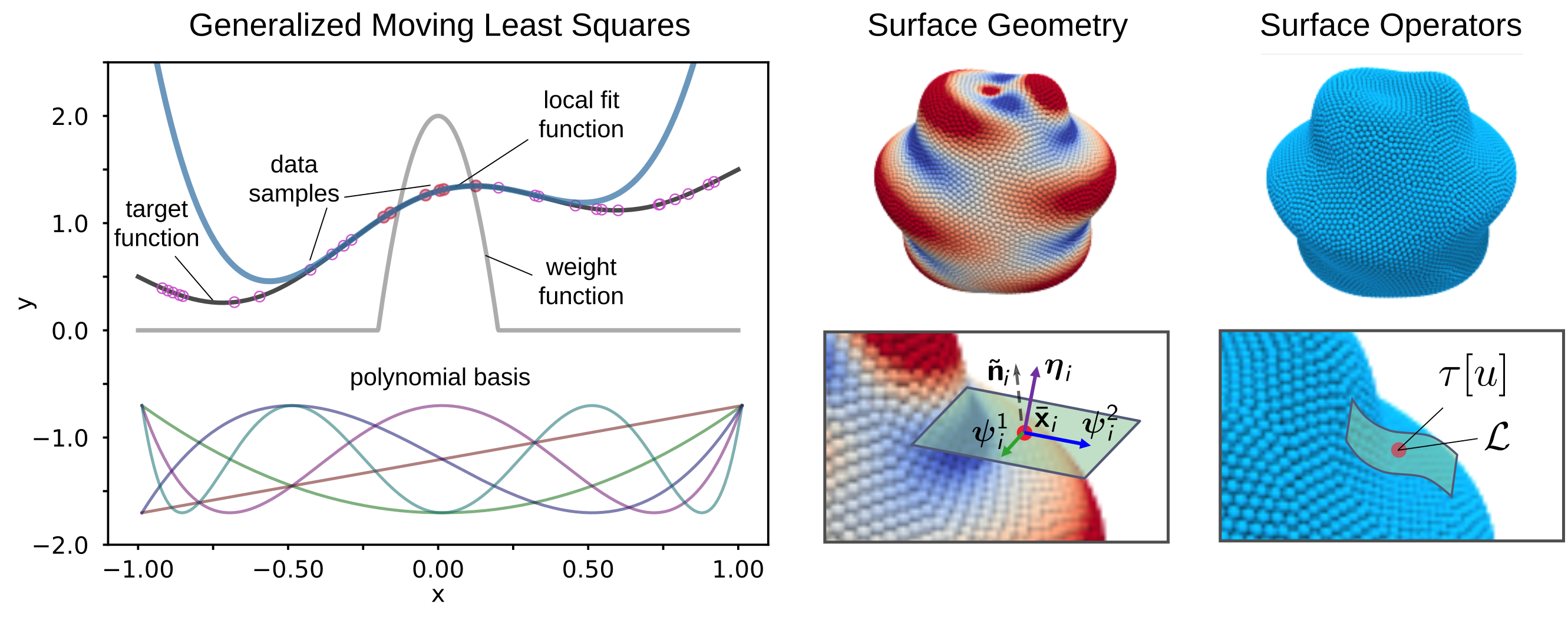
Figure 2: Generalized Moving Least Squares (GMLS) on Surfaces. (left) We approximate the geometry and the action of operators $\tau[u]$ on general surfaces using Generalized Moving Least Squares (GMLS). To approximate a target function $u(\mathbf{x})$ in the neighborhood of a given point $\mathbf{x}^{*}$, GMLS uses the data samples $\{(\mathbf{x}_{j},u(\mathbf{x}_{j}))\}_{j=1}^{m}$, a collection of probing functionals $\{\lambda_{k}[u]\}$, and weights to localize the fit $w(\mathbf{x}^{*},\mathbf{x}_{j})$. These are used to fit locally a function $p^{*}=p^{*}(\mathbf{x})=p^{*}(\mathbf{x};\mathbf{x}^{*})\in\mathbb{V}$. Multivariate polynomials of finite degree are used for the function space $\mathbb{V}$. (middle) Operators are approximated by locally solving related least-squares problems using equations 16 and 18. To handle the geometry at $\mathbf{x}^{*}$, Principle Component Analysis (PCA) is performed using local points to obtain an approximate tangent plane. Geometric quantities are estimated by using GMLS to fit locally the surface in the Monge-Gauge and approximating the related differential operators. Shown is the GMLS estimate of the Gaussian curvature on the surface. (right) The geometric results are used further in conjunction with the GMLS approach to estimate the action of the surface differential operators $\tau[u]=\mathcal{L}u$. Expressions for obtaining geometric quantities in terms of the local surface coordinates are given in Appendix A.

For our first-passage time problems, the target operators are technically non-linear given their dependence on the geometry of the underlying manifold which also must be estimated from the point cloud. We handle this using a two stage approximation approach. In this first stage, we use the point cloud to estimate two basis vectors $\psi_{1}$ and $\psi_{2}$ for the local tangent plane using Principle Component Analysis (PCA) [2, 18]. We use these basis vectors to construct a local coordinate chart $(q_{1},q_{2})$. In this chart, we fit a function $p^{*}\in\mathbb{V}$ to the local point cloud to obtain a Monge-Gauge [19] representation of the surface $(q_{1},q_{2},p^{*}(q_{1},q_{2}))$. We use GMLS to estimate target geometric quantities of interest, such as the local Gaussian curvature or high-order derivatives. In the second stage, we use the estimated geometric quantities to specify the target operators $\tau[u]$ for the fields $u$. We then use again GMLS to obtain an approximation of $\tilde{\tau}$ and to compute numerically the target operator values at $\mathbf{x}_{i}$. We have used related procedures for solving hydrodynamic equations on manifolds in [71]. We illustrate this approximation approach in Figure 2.

2.2 Numerical Methods for Solving the Surface PDEs

To compute numerically the first passage times, we develop solvers for the elliptic PDE boundary value problems given in equation 6. This is organized by representing the $f$ and $g$ function inputs and the $\mathbf{a}$ and $\mathbf{b}$ fields specifying the drift-diffusion dynamics. To avoid complications with local coordinate charts, we numerically represent all input data globally using the ambient embedding space coordinates $\mathbf{x}\in\mathbb{R}^{3}$. The $\mathbf{a}\in\mathbb{R}^{3}$ with only the tangential components playing a role in practice. Similarly, the $\mathbf{b}$ tensor is represented by three vector fields $\mathbf{b_{1}}$, $\mathbf{b_{1}}$, and $\mathbf{b_{3}}$. We use labels on the point cloud to determine which regions are to be considered interior to $\Omega$ and which are part of the boundary of $\partial\Omega$. We only require $f$ to be evaluated on $\partial\Omega$, while $g$ must return reliable values for all $\mathbf{x}\in\Omega$.

We use our GMLS methods in section 2.1 to estimate the surface geometric quantities and the action of the operator in equation 6. This allows us to construct at each $\mathbf{x}_{i}$ an equation for relating $\mathcal{L}u(\mathbf{x}_{i})=-g(\mathbf{x}_{i})$. This provides our collocation method for determining $u(\mathbf{x}_{i})$. Let $[\tilde{u}]_{i}=u(\mathbf{x}_{i})$ and $[\tilde{g}]_{i}=g(\mathbf{x}_{i})$. Collecting these equations together gives a sparse linear system $A\tilde{\mathbf{u}}=\tilde{\mathbf{g}}.$ We solve this large sparse linear system using GMRES with algebraic multigrid (AMG) preconditioning using Trilinos [24]. Our solvers have been implemented within a framework for GMLS problems using the Compadre library and PyCompadre [67]. The toolkit provides domain decomposed distributed vector representation of fields as well as global matrix assembly. The capability of the library were also extended for our surface geometry calculations by implementing symbolically generated target operators. Our methods also made use of the iterative block solvers of (Belos [34]), block preconditioners of (Teko) and the AMG preconditioners of (MueLu [50, 47]) within the Trilinos software framework [24]. The framework facilitates developing a scalable implementation of our methods providing ways to use sparse data structures, parallelization, and hardware accelerations.

3 Convergence Results

We investigate the convergence of our GMLS solvers developed in section 2. The target operators that arise in the surface PDE boundary-value problems involve a non-linear approximation. This arises from the coupling between the contributions to the error from the differential terms of the surface operators and the GMLS estimations used for the surface geometry.

3.1 Surface Geometries for Validation Studies

We perform studies using four different surface geometries: (i) ellipsoid, (ii) radial manifold I, (iii) radial manifold II, and (iv) torus. We label these as Manifold A–D, see Figure 3. We study convergence as the surface point sampling is refined. We take each refinement to have approximately four times the number of points as the previous level. This aims to have the fill distance $h$ halve under each refinement.

The manifolds can be described by the following implicit equations. Manifold A is an ellipsoid defined by the equation ${x^{2}}/{a^{2}}+{y^{2}}/{b^{2}}+z^{2}=s_{0}^{2}$ with $a=1.2,b=1.2,s_{0}^{2}=1$. Manifold B is a radial manifold defined in spherical coordinates by $(\theta,\phi,r(\theta,\phi)$ where $r(\theta,\phi)=1+r_{0}\sin(3\phi)\cos(\theta)$ with $r_{0}=0.1$. Manifold C is a radial manifold defined in spherical coordinates by $(\theta,\phi,r(\theta,\phi)$ where $r(\theta,\phi)=1+r_{0}\sin(7\phi)\cos(\theta)$ with $r_{0}=0.1$. Manifold D is a torus defined by the equation $(s_{1}^{2}-\sqrt{x^{2}+y^{2}})^{2}+z^{2}=s_{2}^{2}$ with $s_{1}^{2}=0.7,s_{2}^{2}=0.3$. Each of the manifolds shown are represented by quasi-uniform point sets with approximately $n=10^{4}$ samples. For quasi-uniform sampling we expect the fill-distance $h$ to scale as $h\sim 1/\sqrt{n}$. We report our results throughout using the notation $\bar{h}^{-1}=\sqrt{n}$. Additional information on the number $n$ used in samplings can be found in Appendix B.

In our first passage time calculations, unless indicated otherwise, we generate the boundary $\partial\Omega$ as the points at $z=0$. In practice, we treat any points with $|z|<4\times 10^{-2}$ as boundary points. This serves to thicken the boundary region and at points $\mathbf{x}_{i}$ near the boundary $\partial\Omega$ helps achieve unisolvency in the local least-squares problems.

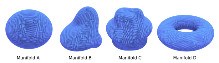
Figure 3: Point Sample Representations of the Surfaces.

3.2 Test Fields and Manufactured Solutions

We study the accuracy of the our GMLS approximations of the surface operators by investigating their action on test fields $\hat{\mathbf{u}}(\mathbf{x})$. We generate $u$ by using smooth functions $\hat{\mathbf{u}}(x,y,z)$ parameterized in the embedding space $\mathbb{R}^{3}$. By the smoothness of the surface manifolds $\mathcal{M}$, evaluation at $\mathbf{x}\in\mathcal{M}$ gives a smooth surface field $u$. More formally, this corresponds to using the inclusion map $\iota:\mathbb{R}^{3}\xhookrightarrow{}\mathcal{M}$ to obtain $\mathbf{u}(\mathbf{x})=\iota_{\mathbf{x}}\hat{\mathbf{u}}(\cdot)$. We also use this inclusion map approach to generate test surface drift tensors $\mathbf{a}$ and diffusion tensors $\mathbf{b}$ for the stochastic process $\mathbf{X}_{t}$ arising in equation 2 and 5.

For our validation studies, we generate test fields $u$ for the Manifolds A–D using $\mathbf{u}(\mathbf{x})=z(x^{4}+y^{4}-6x^{2}y^{2})$, which is an extension of a degree $5$ Spherical Harmonic to $\mathbb{R}^{3}$. For the drift-diffusion tensors for Manifold A, we use

$$\mathbf{a}_{A}=y\tilde{\boldsymbol{\sigma}}_{1}+xz\tilde{\boldsymbol{\sigma}}_{1},\;\;\;\mathbf{b}_{A}=\begin{bmatrix}xz\tilde{\boldsymbol{\sigma}}_{1}+y^{2}\tilde{\boldsymbol{\sigma}}_{2},xyz\tilde{\boldsymbol{\sigma}}_{1}+\cos(y^{2})\tilde{\boldsymbol{\sigma}}_{2},z\tilde{\boldsymbol{\sigma}}_{1}+(y^{3}+x)\tilde{\boldsymbol{\sigma}}_{2}\end{bmatrix}.$$ (19)

The $\tilde{\boldsymbol{\sigma}}_{1},\tilde{\boldsymbol{\sigma}}_{2}$ provide a local orthogonal tangent basis at every point on the Manifold A. In practice in our numerical calculations, this does not need to be smooth in $\mathbf{x}$ and we construct these as convenient using our local tangent plane approximation and Gram-Schmidt orthogonalization [31].

For the Manifolds B and C, we use for the drift-diffusion tensors tangential projections of the vector fields in $\mathbb{R}^{3}$ given by

$$\mathbf{a}_{B,C}=\begin{bmatrix}y,\;xz,\;x^{2}yz\end{bmatrix}^{T},\,\,\,\,\,\,\mathbf{b}_{B,C}=\begin{bmatrix}(xz,xyz,z),\;(y^{2},\cos(y^{2}),y^{3}+x),\;(x^{2}+y,e^{-z},e^{y})\end{bmatrix}^{T}.$$ (20)

For Manifold D, we use drift-diffusion tensors

$$\mathbf{a}_{D}=y\boldsymbol{\sigma}_{u}+xz\boldsymbol{\sigma}_{v},\;\;\;\mathbf{b}_{D}=\begin{bmatrix}\sin(xy)\boldsymbol{\sigma}_{u}+y^{2}\boldsymbol{\sigma}_{v},xyz\boldsymbol{\sigma}_{u}+\cos(y^{2})\boldsymbol{\sigma}_{v},e^{z}\boldsymbol{\sigma}_{u}+(y^{3}+x)\boldsymbol{\sigma}_{v}\end{bmatrix}.$$ (21)

The $\boldsymbol{\sigma}_{u},\boldsymbol{\sigma}_{v}$ provide a basis for the tangent space smooth in $\mathbf{x}$ given by the directional derivatives of the global parameterization $\boldsymbol{\sigma}(u,v)$ of the torus [19]. We characterize the accuracy of the GMLS approximation $\tilde{L}$ of the surface operators $\mathcal{L}$ using the $\ell^{2}$-error

$$\epsilon_{op}^{2}\left(\tilde{L}\right) = \left\|\tilde{L}u-\mathcal{L}u\right\|_{n,2}^{2}=\frac{1}{n}\sum_{i=1}^{n}\left(\tilde{L}u(\mathbf{x}_{i})-\mathcal{L}u(\mathbf{x}_{i})\right)^{2}.$$ (22)

In these studies, we evaluate to high precision the action of the operators $\mathcal{L}$ by symbolic calculations using SymPy [58]. In general, we emphasize that such calculations of expressions symbolically can be prohibitive. Using this approach, we investigate the accuracy of the GMLS approximation of the operator for each of the manifolds. We use the approximation spaces with multivariate polynomials of degree $m\in\{2,4,6\}$. These results are reported in Tables 1– 3.

3.3 Results of Convergence Studies

We performed convergence studies for the Manifolds A–D shapes in Figure 3 with the test fields $u$ and drift-diffusion tensors $\mathbf{a},\mathbf{b}$ discussed in Section 3.2. As the manifold resolution is refined, we study the convergence of the GMLS approximations of the surface operators. For the approximation spaces $\mathbb{V}$, we use multivariate polynomials of degree $m\in\{2,4,6\}$. We estimate the convergence rates using the log-log slope of the error $\epsilon_{op}$ as the fill distance parameter $h$ is varied between levels of refinement. We report these results in Tables 1– 3.

We find in our empirical results that when using GMLS with multinomial spaces of degree $m$ to evaluate the elliptic PDEs operator $\mathcal{L}$ of order $k$, we obtain convergence results of order $m$. We remark that the standard theory does not apply for our surface operators, since there are non-linearities from the coupling between the surface geometry and the differential terms in the operator. Our results are suggestive that our surface operator approximations achieve results exhibiting a trend consistent with simpler differential operators approximated by GMLS [36]. This suggests our methods are resolving the surface geometric contributions with sufficient precision to minimize their contributions to the error. Since the operator $\mathcal{L}$ is of differential order $k=2$ we use throughout approximating polynomial spaces of at least degree $m\geq k\geq 2$.

	Manifold A		Manifold B		Manifold C				Manifold D
h	$\ell_{2}$-error	Rate	$\ell_{2}$-error	Rate	$\ell_{2}$-error	Rate		h	$\ell_{2}$-error	Rate
0.1	2.6503e-02	-	3.6072e-02	-	1.1513e-02	-		.08	8.1920e-03	-
0.05	5.8961e-03	2.14	8.3322e-03	2.11	2.3778e-03	2.27		.04	1.8071e-03	2.21
0.025	1.4951e-03	1.97	2.1451e-03	1.95	6.3865e-04	1.90		.02	4.3928e-04	2.06
0.0125	3.5399e-04	2.07	5.1159e-04	2.06	1.6225e-04	1.98		.01	1.0461e-04	2.05

Table 1: GMLS Convergence Rates for $\mathcal{L}$. For our GMLS methods using approximation spaces based on multivariate polynomials of degree $m=2$, we find convergence rate of $\sim 2^{nd}\mbox{order}$.

	Manifold A		Manifold B		Manifold C				Manifold D
h	$\ell_{2}$-error	Rate	$\ell_{2}$-error	Rate	$\ell_{2}$-error	Rate		h	$\ell_{2}$-error	Rate
0.1	5.8394e-03	-	2.5843e-02	-	5.5971e-03	-		.08	2.5936e-03	-
0.05	2.0355e-04	4.78	1.1594e-03	4.48	3.7890e-04	3.88		.04	1.0359e-04	4.72
0.025	1.1382e-05	4.14	8.2945e-05	3.80	1.9628e-05	4.27		.02	5.4028e-06	4.30
0.0125	6.6746e-07	4.08	5.1207e-06	4.01	1.4226e-06	3.79		.01	3.0733e-07	4.11

Table 2: GMLS Convergence Rates for $\mathcal{L}$. For our GMLS methods using approximation spaces based on multivariate polynomials of degree $m=4$, we find convergence rate of $\sim 4^{th}\mbox{order}$.

	Manifold A		Manifold B		Manifold C				Manifold D
h	$\ell_{2}$-error	Rate	$\ell_{2}$-error	Rate	$\ell_{2}$-error	Rate		h	$\ell_{2}$-error	Rate
0.1	1.8032e-05	-	2.0087e-03	-	2.1854e-03	-		.08	2.7306e-04	-
0.05	2.3775e-07	6.16	5.4584e-05	5.21	1.1625e-04	4.24		.04	2.6141e-06	6.81
0.025	4.3492e-09	5.75	1.4770e-06	5.20	1.5943e-06	6.20		.02	7.4551e-08	5.18
0.0125	6.4443e-11	6.06	1.9655e-08	6.22	3.1347e-08	5.68		.01	1.6423e-09	5.47

Table 3: GMLS Convergence Rates for $\mathcal{L}$. For our GMLS methods using approximation spaces based on multivariate polynomials of degree $m=6$, we find convergence rate of $\sim 6^{th}\mbox{order}$.

4 Results for First Passage Times on Surfaces

For first passage times on surfaces, we investigate the roles played by the geometry, drift dynamics, and spatial-dependence of diffusivity. For our studies, we consider the general surface Langevin dynamics

$$d\mathbf{X}_{t}=-\frac{1}{\gamma}\nabla_{\mathbf{X}}U(\mathbf{X})dt+\sqrt{2D}\mathbf{I}d\mathbf{W}_{t}$$ (23)

$$\mbox{subject to }\mathbf{X}_{t}\in\mathcal{M}.\hskip 73.97733pt$$

The dynamics are expressed here in the embedding space $\mathbf{X}_{t}\in\mathbb{R}^{3}$ and constrained to be within the curved surface $\mathcal{M}$. We could also express these dynamics using local coordinate charts on the surface as discussed in Section 1.1. The $U$ is the potential energy, $\gamma$ the friction coefficient, $D={K_{B}T}/{\gamma}$ the diffusivity, and $K_{B}{T}$ the thermal energy with $K_{B}$ the Boltzmann constant and $T$ the temperature [14]. In terms of the drift-diffusion tensors, $\mathbf{a}(\mathbf{X}_{t})={\gamma}^{-1}\nabla_{\mathbf{X}}U(\mathbf{X}),\;\;\mathbf{b}(\mathbf{X}_{t})=\sqrt{2D}\mathbf{I}$.

4.1 Role of Drift in Mean First Passage Times: Double-Well Potential

Using our methods to capture drift in the surface dynamics, we study the role that can be played by surface potentials in influencing stochastic trajectories and the first passage time. We consider the case of a double-well potential $U$ on a surface which from the conservative force $F=-\nabla_{X}U$ in equation 23 introduces a drift into the dynamics influencing the mean first passage time. We consider geometries $\Omega$ described by the truncated torus, parameterized by

$$\mathbf{X}(u,v)=\begin{bmatrix}\cos(u)(.7+.3\cos(v)),\;\sin(u)(.7+.3\cos(v)),\;.3\sin(v)\end{bmatrix}^{T},\,\,u\in\left[\frac{\pi}{4},\frac{7\pi}{4}\right],\;\;v\in\left[0,2\pi\right).$$

The double-well potential $U$ is generated using the parameterization $(u,v)$ as

$$U(\mathbf{x})=k\sin^{2}(u);\;\;\mathbf{x}=\mathbf{X}(u,v).$$ (24)

We study how the mean first passage time changes as we vary the energy barrier $k=\tilde{k}\cdot k_{B}T$ with $\tilde{k}\in\{0.0,0.05,0.1,0.5,1.0,2.0,5.0\}.$ The case $\tilde{k}=0.0$ serves as our baseline case with no drift. The energy minimum occurs at $u=\pi$ and has energy barriers at $u={\pi}/{2}$ and $u={3\pi}/{2}$ near the boundaries at $u={\pi}/{4}$ and $u={7\pi}/{4}$. We report the results of the first passage times starting at the specific locations $X_{i}$ given by

$$\mathbf{X}_{0}:\left(u,v\right)=\left(\pi,0\right)\;\mathbf{X}_{1}:\left(u,v\right)=\left(\pi,\frac{\pi}{2}\right)\;\mathbf{X}_{2}:\left(u,v\right)=\left(\pi,\pi\right)$$

$$\mathbf{X}_{3}:\left(u,v\right)=\left(\frac{\pi}{2},0\right)\;\mathbf{X}_{4}:\left(u,v\right)=\left(\frac{\pi}{2},\frac{\pi}{2}\right)\;\mathbf{X}_{5}:\left(u,v\right)=\left(\frac{\pi}{2},\pi\right)$$

$$\mathbf{X}_{6}:\left(u,v\right)=\left(\frac{\pi}{3},0\right)\;\mathbf{X}_{7}:\left(u,v\right)=\left(\frac{\pi}{3},\frac{\pi}{2}\right)\;\mathbf{X}_{8}:\left(u,v\right)=\left(\frac{\pi}{3},\pi\right).$$

We report our results in Figure 4.

In our studies the starting locations $X_{0},X_{1},X_{2}$ are at the minimum of the potential energy $U$. From these locations each trajectory must surmount at least one of the energy barriers to reach the boundary. This results in the largest first passage times. We find as the energy barrier is increased $k\gtrsim k_{B}T$ there is approximately exponential increase in the first passage times. This is in agreement with theory for first passage times involving energy barriers based on asymptotic analysis using Kramer’s approximation [6]. Our numerical methods allow for computing the full solution $u(\mathbf{x})$ of equation 3, including first passage times, over a wide range of regimes $k\ll k_{B}T$, $k\sim k_{B}T$, and $k\gg k_{B}T$, and when starting at locations that are not only at the potential energy minimum, see Figure 4.

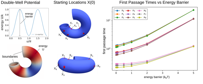
Figure 4: FPTs with Drift-Diffusion Dynamics in Double-Well Potentials. (left) Double-well potential $U$ on the surface of equation 24 influencing the drift of the stochastic dynamics in 23. (middle) The starting locations for first passage times with $\mathbf{X}(0)=\mathbf{X}_{i}$. (right) First passage times from the selected starting points as the strength of the energy barrier $k$ of the double-well potential is varied. The locations $X_{0},X_{1},X_{2}$ start at the minimum of the potential energy and exhibit the longest first passage times. In this case the diffusion must surmount at least one of the energy barriers to reach the boundary. As the energy barrier is increased the first passage times increase, most rapidly when $k\gtrsim k_{B}T$, and with an exponential trend in agreement with Kramer’s theory [6].

4.2 Role of Diffusion in Mean First Passage Times: Spatially-Dependent Diffusivities

We study the role of spatially-dependent heterogeneous diffusivities $b=b(\mathbf{X})$ in first passage times. We consider the surface geometry $\Omega$ obtained from the truncated torus

$$\mathbf{X}(u,v)=\begin{bmatrix}0.4\sin(v),\;\sin(u)(1+0.4\cos(v)),\;-\cos(u)(1+0.4\cos(v))\end{bmatrix}^{T},\;\;u\in\mathcal{U}(z=0,v),v\in\left[0,2\pi\right).$$

This geometry is obtained by slicing the torus at $z=0$. This defines the boundary $\partial\Omega$ and for the parameterization $(u,v)$ a range $\mathcal{U}$ for $u$ that depends on each value of $v$. We consider the spatially-dependent diffusivity

$$\mathbf{b}(\mathbf{x})=\sqrt{2D(\mathbf{x})}\mathbf{I}=\sqrt{2D_{0}}\left(1-c\,\exp\left({\frac{-\|\mathbf{x}-\mathbf{x}_{c}\|^{2}}{r^{2}}}\right)\right)\mathbf{I},$$ (25)

$$\mathbf{x}_{c}:\left(u_{c},v_{c}\right)=\left(\frac{3\pi}{4},\frac{\pi}{2}\right),\;\;\;\;r\geq 0,\;0\leq c<1.$$ (26)

This corresponds in equation 23 to $D=D(\mathbf{x}),\gamma=\gamma(\mathbf{x}),$ and zero drift with $U=0$ so $\mathbf{a}(\mathbf{x})=0$. The exponential is centered at $\mathbf{x}_{c}$ with decay over length-scale $r$ and influence amplitude $c$. For $r$ sufficiently small the variations in diffusivity will occur primarily inside the domain $\Omega$ in a localized region $\|\mathbf{x}-\mathbf{x}_{c}\|\lesssim 3r$. The diffusivity elsewhere will be approximately constant $\sim D$. We consider for our initial starting locations

$$\mathbf{X}_{0}:\left(u,v\right)=\left(\pi,0\right)\;\mathbf{X}_{1}:\left(u,v\right)=\left(\pi,\frac{\pi}{2}\right)\;\mathbf{X}_{2}:\left(u,v\right)=\left(\pi,\pi\right)$$

$$\mathbf{X}_{3}:\left(u,v\right)=\left(\frac{3\pi}{4},0\right)\;\mathbf{X}_{4}:\left(u,v\right)=\left(\frac{3\pi}{4},\frac{\pi}{2}\right)\;\mathbf{X}_{5}:\left(u,v\right)=\left(\frac{3\pi}{4},\pi\right)$$

$$\mathbf{X}_{6}:\left(u,v\right)=\left(\frac{5\pi}{4},0\right)\;\mathbf{X}_{7}:\left(u,v\right)=\left(\frac{5\pi}{4},\frac{\pi}{2}\right)\;\mathbf{X}_{8}:\left(u,v\right)=\left(\frac{5\pi}{4},\pi\right).$$

We study the role of spatially-dependent diffusivity in two cases: (i) when the depth $c$ is varied while leaving the area scale $r$ fixed, and (ii) when the area scale $r$ is varied while leaving the depth $c$ fixed. We use throughout the baseline parameters $c=0.9$ and $r=0.5$. We show the geometry and solution for a typical spatially dependent diffusivity in Figure 5. We report our results in Figure 6.

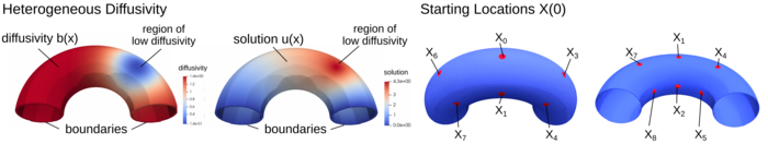
Figure 5: Spatially Dependent Diffusivities. (left) The heterogeneous spatially dependent diffusivity $b(\mathbf{x})$ in equation 25. (left-middle) The solution $u(\mathbf{x})$ for the first passage time problem of equation 6. (right-middle), (right) The starting locations $\mathbf{X}(0)=\mathbf{X}_{i}$. We report results of studies in Figure 6.

We find varying the spatial extent $r$ of the diffusivity plays a particularly strong role in the first passage times. The underlying mechanisms are different than the double-well potential. When a trajectory approaches $\mathbf{x}_{c}$ the motion of the stochastic process slows down significantly as a result of the smaller diffusivity. There is no barrier for $\mathbf{X}_{t}$ to approach such regions but once within this region exhibits a type of temporary trapping behavior from the slow diffusion. We see from Figure 5, such a region influences the first passage time over a much larger range than the direct variations in $b(\mathbf{x})$ given the high probability of a large fraction of trajectories encountering this trapping region even when a modest distance away. We see increases in $r$ have a strong influence on increasing the first passage times, see Figure 6. We also see in the limit that the localized diffusivity $b(\mathbf{x})$ approaches zero, even a relatively small probability of encountering this region can result in a large first passage time. We see this increasing influence as $c$ approaches one, see Figure 6.

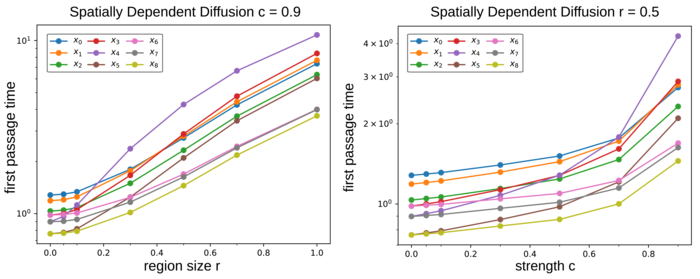
Figure 6: FPTs for Spatially Dependent Diffusivities. (left) The first passage times for the spatially dependent diffusivity $b(\mathbf{x})$ in equation 25 when varying the size $r$ of the region of low diffusivity. (right) The first passage times when increasing the strength $c$ of the diffusivity reduction in equation 25.

4.3 Role of Geometry in Mean First Passage Times: Neck-Shaped Domains

We show how our methods can be used to investigate how the shape of the curved surface influences first passage times. In these studies, we consider purely diffusive dynamics. This corresponds to the case with $U=0$ with zero drift $\mathbf{a}(\mathbf{x})=0$ and a spatially homogeneous diffusivity $\mathbf{b}(\mathbf{x})=\sqrt{2D_{0}}I$ in equation 23. For the geometry we use a surface of revolution with an adjustable shape that forms a neck region near the bottom at $z=0$, see Figure 7. This geometry is generated by considering first a cylinder of radius $r_{0}$ and height $h=0.05$ which is capped at the top by a sphere. We then use a radial profile $r(z)$ to connect the spherical cap with the bottom of the cylinder of radius $r_{0}$ at $z=0$. For this purpose, we use a bump function $r(z)=(1-0.4b)+0.4b\exp\left({1-\frac{b^{2}}{b^{2}-b+.05-z)^{2}}}\right)$. For $z\in[0.05,b+0.05]$, we choose $b$ so that this has arc-length ${\pi}/{2}$, and the final radius $r_{0}$ at $z=0$. This serves to smoothly connect the unit hemisphere cap to the bottom of the cylinder with radius $r_{0}$. This ensures the geodesic distance from $X(0)=X_{i}$ to the boundary is always the same as we vary the shapes, see Figure 7. We report our results in Figure 8.

We find as the neck region becomes smaller it acts as a hindrance for trajectories to reach the boundary and first passage times increase. From the log-log plot we see that the first passage time appears over many radii to follow a power-law trend $\bar{\tau}\sim r^{\alpha}$ with values for $\alpha$ respectively for $X(0)=X_{0},X_{1},X_{2}$ having $\alpha\approx 0.427,0.484,0.893$. As the radius tends to $0$ we see the first passage time diverges. We see for points further from the boundary the first passage times are longer as would be expected. However, as the neck region becomes small, we see smaller differences occur between points $X_{0},X_{1}$ starting at points above the neck region, compared to the point $X_{3}$ starting within the neck region. This indicates that as the radius shrinks the neck region increasingly acts as a hindrance for reaching the boundary. Interesting, we also see that starting at $X_{3}$ also has FPTs that significantly increase, since as $r_{0}\rightarrow 0$ an increasingly large fraction of trajectories will leave the neck region before encountering the boundary and then must also overcome the hindrance similar to starting at $X_{0},X_{1}$. We can characterize this mechanism by using a reaction-coordinate and notion of free energy (entropy contributions) arising from the constricting geometry.

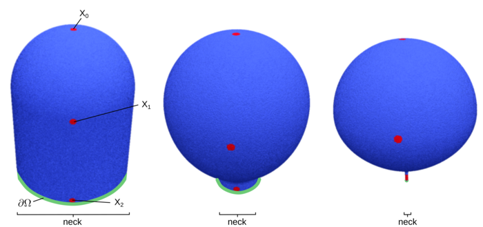
Figure 7: Neck Geometries for First Passage Time Studies. For the FPT studies when varying the geometry of the neck region, we show the select starting locations $\mathbf{X}(0)=\mathbf{X}_{i}$ (red points). On the left we show the largest neck domain which does not present a geometric bottleneck for reaching the $\partial\Omega$ at $z=0$. On the right, we show the smallest neck region which presents a significant geometric bottleneck potentially inhibiting diffusion in reaching $z=0$. The geometries used in these studies were designed so that as the neck width is varied the geodesic distance from the starting points remains constant to reach the boundary $\partial\Omega$ at $z=0$.

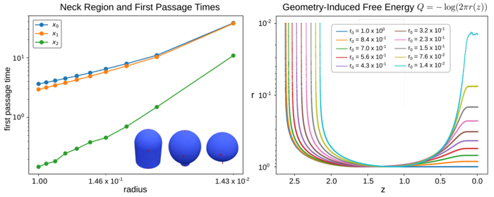
Figure 8: FPTs Dependence on the Neck Geometry. (left) The first passage time as the neck radius $r$ becomes small. We see as the neck becomes narrower (towards the right) the geometry of the manifold restricts the diffusion and reaching the boundary becomes more difficult. The $r$ indicates the narrowest radius of the shape. (right) The shape acts to give a geometrically induced free energy $Q(z)=-log(2\pi r(z))$ for the dynamics when projecting to the $z$-axis. We see as the neck radius $r$ narrows (towards the right) the geometry creates an increasingly large free-energy barrier and increases the first-passage times.

Given the radial symmetry we can project the stochastic dynamics onto the $z$-component as an effective reaction-coordinate for reaching the boundary at $z=0$. This provides a statistical mechanics model [14] where the shape of the manifold gives an effective free energy having entropic contributions proportional to $Q(z)=-\log(2\pi r(z))$. This contributes to an effective mean-force for $Z_{t}$ yielding the drift $a(z)=-\partial Q/\partial z=-Q^{\prime}(z)$. This suggests the radially-averaged stochastic dynamics $dZ_{t}=-Q^{\prime}(Z_{t})dt+C\,dW_{t}.$ From this perspective, the drift-diffusion process $Z_{t}$ must cross the geometrically-induced energy barrier $Q(z)$ to reach the boundary at $z=0$. Similar to our results on double-well potentials, this could be studied analytically with asymptotic Kramer’s theory [6]. Our numerical methods allow for capturing directly these effects and we see as the neck narrows this significantly increases the first passage times. This correlates well with how the effective free energy barrier for $Z_{t}$ increases with the shape change, see Figure 8. Our results show how geometric effects captured by our methods can provide mechanisms that influence significantly the behaviors of stochastic processes and their first passage times.

Conclusions

We have developed numerical methods for computing the mean First Passage Times and related path-dependent statistics of stochastic processes on surfaces of general shape and topology. We formulated descriptions of Brownian motion and general drift-diffusion processes on surfaces. Using Dynkin’s formula and Backward-Kolmogorov equations of these processes, we formulated and solved associated elliptic PDE boundary value problems on curved surfaces. We developed our numerical methods using Generalized Moving Least Squares (GMLS) to approximate the local surface geometry and the action of surface differential operators. Using this discretization approach we introduced collocation methods and solvers for the associated linear systems of equations. For a variety of surface shapes, we showed that our methods converge with high-order accuracy in capturing the geometry and PDE solutions. For mean First Passage Times, we showed how our methods can be used to investigate the roles of the surface geometry, drift dynamics, and spatially dependent diffusivities. The solvers and approaches we have developed also can be used more generally to compute other path-dependent statistics and solutions to elliptic boundary-value problems on surfaces of general shape.

Appendix

Appendix A Monge-Gauge Surface Parameterization

In the Monge-Gauge we parameterize locally a smooth surface in terms of the tangent plane coordinates $u,v$ and the height of the surface above this point as the function $h(u,v)$. This gives the embedding map

$$\mathbf{x}(u,v)=\boldsymbol{\sigma}(u,v)=(u,v,h(u,v)).$$ (27)

We can use the Monge-Gauge equation 27 to derive explicit expressions for geometric quantities. The derivatives of $\boldsymbol{\sigma}$ provide a basis $\partial_{u},\partial_{v}$ for the tangent space as

$$\partial_{u}=\boldsymbol{\sigma}_{u}(u,v) = (1,0,h_{u}(u,v))$$ (28)

$$\partial_{v}=\boldsymbol{\sigma}_{v}(u,v) = (0,1,h_{v}(u,v)).$$ (29)

The first fundamental form $\mathbf{I}$ (metric tensor) and its inverse $\mathbf{I}^{-1}$ (inverse tensor) are given by

$$\mathbf{I}=\begin{bmatrix}g_{uu}&g_{uv}\\ g_{vu}&g_{vv}\end{bmatrix}=\begin{bmatrix}\boldsymbol{\sigma}_{u}\cdot\boldsymbol{\sigma}_{u}&\boldsymbol{\sigma}_{u}\cdot\boldsymbol{\sigma}_{v}\\ \boldsymbol{\sigma}_{v}\cdot\boldsymbol{\sigma}_{u}&\boldsymbol{\sigma}_{v}\cdot\boldsymbol{\sigma}_{v}\end{bmatrix}=\begin{bmatrix}1+h_{u}(u,v)^{2}&h_{u}h_{v}(u,v)\\ h_{u}(u,v)h_{v}(u,v)&1+h_{v}(u,v)^{2}\end{bmatrix}.$$ (30)

and

$$\mathbf{I}^{-1}=\begin{bmatrix}g^{uu}&g^{uv}\\ g^{vu}&g^{vv}\end{bmatrix}=\frac{1}{1+h_{u}^{2}+h_{v}^{2}}\begin{bmatrix}1+h_{v}^{2}&-h_{u}h_{v}\\ -h_{u}h_{v}&1+h_{u}^{2}\end{bmatrix}.$$ (31)

We use throughout the notation for the metric tensor $\mathbf{g}=\mathbf{I}$ interchangeably. For notational convenience, we use the tensor notation for the metric tensor $g_{ij}$ and for its inverse $g^{ij}$. These correspond to the first fundamental form and its inverse as

$$g_{ij}=\left[\mathbf{I}\right]_{i,j},\hskip 8.5359ptg^{ij}=\left[\mathbf{I}^{-1}\right]_{i,j}.$$ (32)

For the metric tensor $\mathbf{g}$, we also use the notation $|g|=\det(\mathbf{g})$ and have that

$$\sqrt{|g|}=\sqrt{\det(\mathbf{I})}=\sqrt{1+h_{u}^{2}+h_{v}^{2}}=\|\mathbf{\sigma}_{u}(u,v)\times\mathbf{\sigma}_{v}(u,v)\|.$$ (33)

The provides the local area element as $dA_{u,v}=\sqrt{|g|}dudv$.

The Christoffel symbols of the second kind were used in our derivations of Brownian motion and more general stochastic drift-diffusion dynamics on surfaces. In the general case, the Christoffel symbols are given by

$$\Gamma^{k}_{ij}=\partial_{j}\boldsymbol{\sigma}_{i}\cdot\boldsymbol{\sigma}_{k}.$$ (34)

In the case of the Monge-Gauge $\boldsymbol{\sigma}(u,v)=(u,v,h(u,v)$, this can be expressed as

$$\Gamma^{k}_{ij}=\frac{h_{ij}h_{k}}{\sqrt{|g|}}=\frac{h_{ij}h_{k}}{\sqrt{1+h_{u}^{2}+h_{v}^{2}}}.$$ (35)

To compute quantities associated with curvature of the manifold, we construct the Weingarten map [19]. This can be expressed as

$$\mathbf{W}=\mathbf{I}^{-1}\mathbf{II}.$$ (36)

The Gaussian curvature $K$ can be expressed in the Monge-Gauge as

$$K(u,v)=\det\left(\mathbf{W}(u,v)\right)=\frac{h_{uu}h_{vv}-h_{uv}^{2}}{(1+h_{u}^{2}+h_{v}^{2})^{2}}.$$ (37)

For further discussions on the differential geometry of manifolds and computation of surface operators see [19, 7, 16, 71].

Appendix B Sampling Resolution of the Manifolds

We provide a summary of the sampling resolution $h$ used for each of the manifolds in Table 4. We refer to $h$ as the target fill distance. For each of the manifolds and target spacing $h$, we achieve a nearly uniform collection of the points (quasi-uniform samplings) using DistMesh [22]. In practice, we have found this yields a point spacing with neighbor distances varying by about $\approx\pm 30\%$ relative to the target distance $h$. We summarize for each of the manifolds how this relates to the number of sample points $n$ in Table 4. Robustness studies for related solvers have been carried out when applying perturbations to such point samples in [71].

Refinement Level	A: h	n	B: h	n	C: h	n	D: h	n
$1$	.1	2350	.1	2306	.1	2002	.08	1912
$2$	.05	9566	.05	9206	.05	7998	.04	7478
$3$	.025	38486	.025	36854	.025	31898	.02	29494
$4$	.0125	154182	.0125	147634	.0125	127346	.01	118942

Table 4: Sampling Resolution for each of the Manifolds A–D. Relation between the target distance $h$ and the number of sample points $n$ used for each of the manifolds. In each case, the neighbor distances between the points sampled were within $\approx\pm 30\%$ of the target distance $h$.

References

- [1] Louis Bachelier “Théorie de la spéculation” In Annales scientifiques de l’École Normale Supérieure 3e série, 17 Elsevier, 1900, pp. 21–86 DOI: 10.24033/asens.476
- [2] Karl Pearson F.R.S. “LIII. On lines and planes of closest fit to systems of points in space” In The London, Edinburgh, and Dublin Philosophical Magazine and Journal of Science 2.11 Taylor & Francis, 1901, pp. 559–572 DOI: 10.1080/14786440109462720
- [3] G. Klein and Max Born “Mean first-passage times of Brownian motion and related problems” In Proceedings of the Royal Society of London. Series A. Mathematical and Physical Sciences 211.1106, 1952, pp. 431–443 DOI: 10.1098/rspa.1952.0051
- [4] Robert A Gingold and Joseph J Monaghan “Smoothed particle hydrodynamics: theory and application to non-spherical stars” In Monthly notices of the royal astronomical society 181.3 Oxford University Press Oxford, UK, 1977, pp. 375–389
- [5] Peter Lancaster and Kes Salkauskas “Surfaces generated by moving least squares methods” In Mathematics of computation 37.155, 1981, pp. 141–158
- [6] C. W. Gardiner “Handbook of stochastic methods”, Series in Synergetics Springer, 1985
- [7] R. Abraham, J.E. Marsden and T.S. Ratiu “Manifolds, Tensor Analysis, and Applications” Springer New York, 1988 URL: https://books.google.com/books?id=dWHet_zgyCAC
- [8] Derek Y. C. Chan and Donald A. McQuarrie “Mean first passage times of ions between charged surfaces” In J. Chem. Soc., Faraday Trans. 86 The Royal Society of Chemistry, 1990, pp. 3585–3595 DOI: 10.1039/FT9908603585
- [9] E.J. Kansa “Multiquadrics-A scattered data approximation scheme with applications to computational fluid-dynamics—I surface approximations and partial derivative estimates” In Computers & Mathematics with Applications 19.8, 1990, pp. 127–145 DOI: https://doi.org/10.1016/0898-1221(90)90270-T
- [10] E.J. Kansa “Multiquadrics-A scattered data approximation scheme with applications to computational fluid-dynamics—II solutions to parabolic, hyperbolic and elliptic partial differential equations” In Computers & Mathematics with Applications 19.8, 1990, pp. 147–161 DOI: https://doi.org/10.1016/0898-1221(90)90271-K
- [11] Kloeden.P.E. and E. Platen “Numerical solution of stochastic differential equations” Springer-Verlag, 1992
- [12] Wing Kam Liu, Sukky Jun and Yi Fei Zhang “Reproducing kernel particle methods” In International Journal for Numerical Methods in Fluids 20.8-9, 1995, pp. 1081–1106 DOI: https://doi.org/10.1002/fld.1650200824
- [13] Reinhard Müller, Peter Talkner and Peter Reimann “Rates and mean first passage times” In Physica A: Statistical Mechanics and its Applications 247.1, 1997, pp. 338 –356 DOI: https://doi.org/10.1016/S0378-4371(97)00390-7
- [14] L. E. Reichl “A Modern Course in Statistical Physics” John WileySons, 1998
- [15] M Newman and G Barkema “Monte carlo methods in statistical physics” Oxford University Press: New York, USA, 1999
- [16] Micheal Spivak “A Comprehensive Introduction to Differential Geometry” Publish or Perish Inc., 1999
- [17] B. Oksendal “Stochastic Differential Equations: An Introduction” Springer, 2000
- [18] Trevor Hastie, Robert Tibshirani and Jerome Friedman “Elements of Statistical Learning”, Springer Series in Statistics New York, NY, USA: Springer New York Inc., 2001
- [19] A. Pressley “Elementary Differential Geometry” Springer, 2001 URL: https://books.google.com/books?id=UXPyquQaO6EC
- [20] Sidney Redner “A Guide to First-Passage Processes” Cambridge University Press, 2001 DOI: 10.1017/CBO9780511606014
- [21] Martin D Buhmann “Radial basis functions: theory and implementations” Cambridge university press, 2003
- [22] Per-Olof Persson and Gilbert Strang “A Simple Mesh Generator in MATLAB” In SIAM Review 46.2 SIAM, 2004, pp. 329–345
- [23] Holger Wendland “Scattered data approximation” Cambridge university press, 2004
- [24] Michael A. Heroux, Roscoe A. Bartlett, Vicki E. Howle, Robert J. Hoekstra, Jonathan J. Hu, Tamara G. Kolda, Richard B. Lehoucq, Kevin R. Long, Roger P. Pawlowski, Eric T. Phipps, Andrew G. Salinger, Heidi K. Thornquist, Ray S. Tuminaro, James M. Willenbring, Alan Williams and Kendall S. Stanley “An Overview of the Trilinos Project” In ACM Trans. Math. Softw. 31.3 New York, NY, USA: ACM, 2005, pp. 397–423 DOI: 10.1145/1089014.1089021
- [25] John B. Greer, Andrea L. Bertozzi and Guillermo Sapiro “Fourth Order Partial Differential Equations on General Geometries” In J. Comput. Phys. 216.1 San Diego, CA, USA: Academic Press Professional, Inc., 2006, pp. 216–246 DOI: 10.1016/j.jcp.2005.11.031
- [26] Russ Tedrake, Katie Byl and JE Pratt “Probabilistic stability in legged systems: Metastability and the mean first passage time (FPT) stability margin” In arXiv Citeseer, 2006
- [27] Jérôme Callut and Pierre Dupont “Learning Partially Observable Markov Models from First Passage Times” In Proceedings of the 18th European Conference on Machine Learning, ECML ’07 Warsaw, Poland: Springer-Verlag, 2007, pp. 91–103 DOI: 10.1007/978-3-540-74958-5˙12
- [28] Thomas-Peter Fries and Ted Belytschko “Convergence and stabilization of stress-point integration in mesh-free and particle methods” In International Journal for Numerical Methods in Engineering 74.7 Wiley Online Library, 2008, pp. 1067–1087
- [29] Steven J. Ruuth and Barry Merriman “A simple embedding method for solving partial differential equations on surfaces” In Journal of Computational Physics 227.3, 2008, pp. 1943–1961 DOI: https://doi.org/10.1016/j.jcp.2007.10.009
- [30] J. Hull “Options, Futures and Other Derivatives”, Prentice Hall finance series Pearson/Prentice Hall, 2009 URL: https://books.google.com/books?id=sEmQZoHoJCcC
- [31] Richard L. Burden and Douglas Faires “Numerical Analysis” Brooks/Cole Cengage Learning, 2010
- [32] Bengt Fornberg and Erik Lehto “Stabilization of RBF-generated finite difference methods for convective PDEs” In Journal of Computational Physics 230.6 Elsevier, 2011, pp. 2270–2285
- [33] Shingyu Leung, John Lowengrub and Hongkai Zhao “A grid based particle method for solving partial differential equations on evolving surfaces and modeling high order geometrical motion” In Journal of Computational Physics 230.7, 2011, pp. 2540 –2561 DOI: https://doi.org/10.1016/j.jcp.2010.12.029
- [34] Eric Bavier, Mark Hoemmen, Sivasankaran Rajamanickam and Heidi Thornquist “Amesos2 and Belos: Direct and iterative solvers for large sparse linear systems” In Scientific Programming 20.3, 2012
- [35] Natasha Flyer, Erik Lehto, Sébastien Blaise, Grady B Wright and Amik St-Cyr “A guide to RBF-generated finite differences for nonlinear transport: Shallow water simulations on a sphere” In Journal of Computational Physics 231.11 Elsevier, 2012, pp. 4078–4095
- [36] D. Mirzaei, R. Schaback and M. Dehghan “On generalized moving least squares and diffuse derivatives” In IMA Journal of Numerical Analysis 32.3, 2012, pp. 983–1000 DOI: 10.1093/imanum/drr030
- [37] Cécile Piret “The Orthogonal Gradients Method: A Radial Basis Functions Method for Solving Partial Differential Equations on Arbitrary Surfaces” In J. Comput. Phys. 231.14 San Diego, CA, USA: Academic Press Professional, Inc., 2012, pp. 4662–4675 DOI: 10.1016/j.jcp.2012.03.007
- [38] Edward J. Fuselier and Grady B. Wright “A High-Order Kernel Method for Diffusion and Reaction-Diffusion Equations on Surfaces” In Journal of Scientific Computing 56.3, 2013, pp. 535–565 DOI: 10.1007/s10915-013-9688-x
- [39] Gutiérrez “American option valuation using first-passage densities” In Quantitative Finance 13.11 Routledge, 2013, pp. 1831–1843 DOI: 10.1080/14697688.2013.794387
- [40] Jian Liang and Hongkai Zhao “Solving partial differential equations on point clouds” In SIAM Journal on Scientific Computing 35.3 SIAM, 2013, pp. A1461–A1486
- [41] Jian Liang and Hongkai Zhao “Solving partial differential equations on point clouds” In SIAM Journal on Scientific Computing 35.3 SIAM, 2013, pp. A1461–A1486
- [42] Colin B. Macdonald, Barry Merriman and Steven J. Ruuth “Simple computation of reaction-diffusion processes on point clouds.” In Proceedings of the National Academy of Sciences of the United States of America 110, 2013, pp. 9209–14 URL: https://www.pnas.org/content/110/23/9209
- [43] Thibaud Taillefumier and Marcelo O. Magnasco “A phase transition in the first passage of a Brownian process through a fluctuating boundary with implications for neural coding” In Proceedings of the National Academy of Sciences 110.16 National Academy of Sciences, 2013, pp. E1438–E1443 DOI: 10.1073/pnas.1212479110
- [44] E. Ben-Naim and P. L. Krapivsky “First Passage in Conical Geometry and Ordering of Brownian Particles” In First-Passage Phenomena and Their Applications World Scientific, 2014, pp. 252–276 DOI: 10.1142/9789814590297˙0011
- [45] Rémy Chicheportiche and Jean-Philippe Bouchaud “Some Applications of First-Passage Ideas to Finance” In First-Passage Phenomena and Their Applications World Scientific, 2014, pp. 447–476 DOI: 10.1142/9789814590297˙0018
- [46] T. Chou and M. R. D’Orsogna “First Passage Problems in Biology” In First-Passage Phenomena and Their Applications World Scientific, 2014, pp. 306–345 DOI: 10.1142/9789814590297˙0013
- [47] Jonathan J. Hu, Andrey Prokopenko, Christopher M. Siefert, Raymond S. Tuminaro and Tobias A. Wiesner “MueLu multigrid framework”, http://trilinos.org/packages/muelu, 2014
- [48] Remy Kusters and Cornelis Storm “Impact of morphology on diffusive dynamics on curved surfaces” In Phys. Rev. E 89 American Physical Society, 2014, pp. 032723 URL: https://link.aps.org/doi/10.1103/PhysRevE.89.032723
- [49] Ava J. Mauro, Jon Karl Sigurdsson, Justin Shrake, Paul J. Atzberger and Samuel A. Isaacson “A First-Passage Kinetic Monte Carlo method for reaction–drift–diffusion processes” In Journal of Computational Physics 259, 2014, pp. 536 –567 DOI: https://doi.org/10.1016/j.jcp.2013.12.023
- [50] Andrey Prokopenko, Jonathan J. Hu, Tobias A. Wiesner, Christopher M. Siefert and Raymond S. Tuminaro “MueLu User’s Guide 1.0”, 2014
- [51] Cenk Oguz Saglam and Katie Byl “First Passage Value” In arXiv, 2014 arXiv:1412.6704 [cs.SY]
- [52] O Bénichou, T Guérin and R Voituriez “Mean first-passage times in confined media: from Markovian to non-Markovian processes” In Journal of Physics A: Mathematical and Theoretical 48.16 IOP Publishing, 2015, pp. 163001 DOI: 10.1088/1751-8113/48/16/163001
- [53] Varun Shankar, Grady B. Wright, Robert M. Kirby and Aaron L. Fogelson “A Radial Basis Function (RBF)-Finite Difference (FD) Method for Diffusion and Reaction–Diffusion Equations on Surfaces” In Journal of Scientific Computing 63.3, 2015, pp. 745–768 DOI: 10.1007/s10915-014-9914-1
- [54] Nicholas F. Polizzi, Michael J. Therien and David N. Beratan “Mean First-Passage Times in Biology.” In Israel journal of chemistry 56, 2016, pp. 816–824
- [55] Khem Raj Ghusinga, John J. Dennehy and Abhyudai Singh “First-passage time approach to controlling noise in the timing of intracellular events” In Proceedings of the National Academy of Sciences National Academy of Sciences, 2017 DOI: 10.1073/pnas.1609012114
- [56] C. Hohenegger, R. Durr and D.M. Senter “Mean first passage time in a thermally fluctuating viscoelastic fluid” In Journal of Non-Newtonian Fluid Mechanics 242, 2017, pp. 48 –56 DOI: https://doi.org/10.1016/j.jnnfm.2017.03.001
- [57] Alan E. Lindsay, Andrew J. Bernoff and Michael J. Ward “First Passage Statistics for the Capture of a Brownian Particle by a Structured Spherical Target with Multiple Surface Traps” In Multiscale Modeling & Simulation 15.1, 2017, pp. 74–109 DOI: 10.1137/16M1077659
- [58] Aaron Meurer, Christopher P. Smith, Mateusz Paprocki, Ondřej Čertík, Sergey B. Kirpichev, Matthew Rocklin, AMiT Kumar, Sergiu Ivanov, Jason K. Moore, Sartaj Singh, Thilina Rathnayake, Sean Vig, Brian E. Granger, Richard P. Muller, Francesco Bonazzi, Harsh Gupta, Shivam Vats, Fredrik Johansson, Fabian Pedregosa, Matthew J. Curry, Andy R. Terrel, Štěpán Roučka, Ashutosh Saboo, Isuru Fernando, Sumith Kulal, Robert Cimrman and Anthony Scopatz “SymPy: symbolic computing in Python” In PeerJ Computer Science 3, 2017, pp. e103 DOI: 10.7717/peerj-cs.103
- [59] Ka Chun Cheung and Leevan Ling “A kernel-based embedding method and convergence analysis for surfaces PDEs” In SIAM Journal on Scientific Computing 40.1 SIAM, 2018, pp. A266–A287
- [60] S. Debnath, L. Liu and G. Sukhatme “Solving Markov Decision Processes with Reachability Characterization from Mean First Passage Times” In 2018 IEEE/RSJ International Conference on Intelligent Robots and Systems (IROS), 2018, pp. 7063–7070 DOI: 10.1109/IROS.2018.8594383
- [61] Denis S. Grebenkov, Ralf Metzler and Gleb Oshanin “Strong defocusing of molecular reaction times results from an interplay of geometry and reaction control” In Communications Chemistry 1.1, 2018, pp. 96 URL: https://doi.org/10.1038/s42004-018-0096-x
- [62] A. Petras, L. Ling and S.J. Ruuth “An RBF-FD closest point method for solving PDEs on surfaces” In Journal of Computational Physics 370, 2018, pp. 43 –57 DOI: https://doi.org/10.1016/j.jcp.2018.05.022
- [63] Varun Shankar, Akil Narayan and Robert M. Kirby “RBF-LOI: Augmenting Radial Basis Functions (RBFs) with Least Orthogonal Interpolation (LOI) for solving PDEs on surfaces” In Journal of Computational Physics 373, 2018, pp. 722 –735 DOI: https://doi.org/10.1016/j.jcp.2018.07.015
- [64] Varun Shankar and Grady B. Wright “Mesh-free semi-Lagrangian Methods for Transport on a Sphere Using Radial Basis Functions” In J. Comput. Phys. 366.C San Diego, CA, USA: Academic Press Professional, Inc., 2018, pp. 170–190 DOI: 10.1016/j.jcp.2018.04.007
- [65] Marino Arroyo Alejandro Torres-Sanchez “Approximation of tensor fields on surfaces of arbitrary topology based on local Monge parametrizations” In arXiv, 2019 URL: https://arxiv.org/abs/1904.06390
- [66] Adam Kells, Zsuzsanna É. Mihálka, Alessia Annibale and Edina Rosta “Mean first passage times in variational coarse graining using Markov state models” In The Journal of Chemical Physics 150.13, 2019, pp. 134107 DOI: 10.1063/1.5083924
- [67] Paul Kuberry, Peter Bosler and Nathaniel Trask “Compadre Toolkit”, 2019 DOI: 10.11578/dc.20190411.1
- [68] Vahid Mohammadi, Mehdi Dehghan, Amirreza Khodadadian and Thomas Wick “Generalized moving least squares and moving kriging least squares approximations for solving the transport equation on the sphere” In arXiv, 2019 URL: https://arxiv.org/abs/1904.05831
- [69] Joerg Kuhnert Pratik Suchde “A Fully Lagrangian Meshfree Framework for PDEs on Evolving Surfaces” In arXiv, 2019
- [70] Junhong Xu, Kai Yin and Lantao Liu “Reachable Space Characterization of Markov Decision Processes with Time Variability”, 2019 arXiv:1905.09342 [cs.RO]
- [71] B.J. Gross, N. Trask, P. Kuberry and P. J. Atzberger “Meshfree methods on manifolds for hydrodynamic flows on curved surfaces: A Generalized Moving Least-Squares (GMLS) approach” In Journal of Computational Physics 409 Elsevier, 2020 URL: https://doi.org/10.1016/j.jcp.2020.109340
- [72] Nathaniel Trask and Paul Kuberry “Compatible meshfree discretization of surface PDEs” In Computational Particle Mechanics 7.2, 2020, pp. 271–277 URL: https://doi.org/10.1007/s40571-019-00251-2
- [73] Patrick D. Tran, Thomas A. Blanpied and Paul J. Atzberger “Drift-Diffusion Dynamics and Phase Separation in Curved Cell Membranes and Dendritic Spines: Hybrid Discrete-Continuum Methods”, 2021 arXiv:2110.00725 [physics.bio-ph]