Learning Noise Transition Matrix from Only Noisy Labels
via Total Variation Regularization

Abstract

Many weakly supervised classification methods employ a noise transition matrix to capture the class-conditional label corruption. To estimate the transition matrix from noisy data, existing methods often need to estimate the noisy class-posterior, which could be unreliable due to the overconfidence of neural networks. In this work, we propose a theoretically grounded method that can estimate the noise transition matrix and learn a classifier simultaneously, without relying on the error-prone noisy class-posterior estimation. Concretely, inspired by the characteristics of the stochastic label corruption process, we propose total variation regularization, which encourages the predicted probabilities to be more distinguishable from each other. Under mild assumptions, the proposed method yields a consistent estimator of the transition matrix. We show the effectiveness of the proposed method through experiments on benchmark and real-world datasets.

[name=Theorem]theorem

1 Introduction

Can we learn a correct classifier based on possibly incorrect examples? The study of classification in the presence of label noise has been of interest for decades (Angluin & Laird, 1988) and is becoming more important in the era of deep learning (Goodfellow et al., 2016). This issue can be caused by the use of imperfect surrogates of clean labels produced by annotation techniques for large-scale datasets such as crowdsourcing and web crawling (Fergus et al., 2005; Jiang et al., 2020). Unfortunately, without proper regularization, deep models could be more vulnerable to overfitting the label noise in the training data (Arpit et al., 2017; Zhang et al., 2017), which affects the classification performance adversely.

Background.

Early studies on learning from noisy labels can be traced back to the random classification noise (RCN) model for binary classification (Angluin & Laird, 1988; Long & Servedio, 2010; Van Rooyen et al., 2015). Then, RCN has been extended to the case where the noise rate depends on the classes, called the class-conditional noise (CCN) model (Natarajan et al., 2013). The multiclass case is of central interest in recent years (Patrini et al., 2017; Goldberger & Ben-Reuven, 2017; Han et al., 2018a; Xia et al., 2019; Yao et al., 2020), where multiclass labels $Y$ flip into other categories ${\widetilde{Y}}$ according to probabilities described by a fixed but unknown noise transition matrix ${\bm{T}}$, where ${\bm{T}}_{ij}=p({\widetilde{Y}}=j|Y=i)$. In this work, we focus on the multiclass CCN model. Other noise models are discussed in Appendix A.

Methodology.

The unknown noise transition matrix in CCN has become a hurdle. In this work, we focus on a line of research that aims to estimate the transition matrix from noisy data. With a consistently estimated transition matrix, consistent estimation of the clean class-posterior is possible (Patrini et al., 2017). To estimate the transition matrix, earlier work mainly relies on a given set of anchor points (Liu & Tao, 2015; Patrini et al., 2017; Yu et al., 2018), i.e., instances belonging to the true class deterministically. With anchor points, the transition matrix becomes identifiable based on the noisy class-posterior. Further, recent work has attempted to detect anchor points in noisy data to mitigate the lack of anchor points in real-world settings (Xia et al., 2019; Yao et al., 2020).

Nevertheless, even with a given anchor point set, these two-step methods of first estimating the transition matrix and then using it in neural network training face an inevitable problem — the estimation of the noisy class-posterior. The estimation error could be high due to the overconfidence of neural networks (Guo et al., 2017; Hein et al., 2019; Rahimi et al., 2020) (see also Appendix B).

In this work, we present an alternative methodology that does not rely on the error-prone estimation of the noisy class-posterior. The key idea is as follows: Note the fact that the noisy class-posterior vector is given by the product of the noise transition matrix ${\bm{T}}$ and the clean class-posterior vector ${\bm{p}}$: $\rm={\bm{T}}^{\mathsf{T}}{\bm{p}}$. However, in the reverse direction, the decomposition of the product is not always unique, so ${\bm{T}}$ and ${\bm{p}}$ are not identifiable from . Thus, without additional assumption, existing methods for estimating ${\bm{T}}$ from could be unreliable. However, if ${\bm{p}}$ has some characteristics, e.g., ${\bm{p}}$ is the “cleanest” among all the possibilities, then ${\bm{T}}$ and ${\bm{p}}$ become identifiable and it is possible to construct consistent estimators. Concretely, we assume that anchor points exist in the dataset to guarantee the identifiability, but we do not need to explicitly model or detect them (Section 3.2).

Further, note that the mapping ${\bm{p}}\mapsto{\bm{T}}^{\mathsf{T}}{\bm{p}}$ is a contraction over the probability simplex relative to the total variation distance (Del Moral et al., 2003). That is, the “cleanest” ${\bm{p}}$ has the property that pairs of ${\bm{p}}$ are more distinguishable from each other. Based on this motivation, we propose total variation regularization to find the “cleanest” ${\bm{p}}$ and consistently estimate ${\bm{T}}$ simultaneously (Section 4.1).

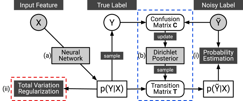
Figure 1: An illustration of the proposed method. Our model has two modules: (a) a neural network for predicting ${\bm{p}}(Y|X)$; and (b) a Dirichlet posterior for the noise transition matrix ${\bm{T}}$, whose concentration parameters are updated using the confusion matrix obtained during training. The learning objective in Eq. 12 also contains two parts: (i) the usual cross entropy loss for classification from noisy labels in Eq. 5; and (ii) a total variation regularization term for the predicted probability in Eq. 10.

Our contribution.

In this paper, we study the class-conditional noise (CCN) problem and propose a method that can estimate the noise transition matrix and learn a classifier simultaneously, given only noisy data. The key idea is to regularize the predicted probabilities to be more distinguishable from each other using the pairwise total variation distance. Under mild conditions, the transition matrix becomes identifiable and a consistent estimator can be constructed.

Specifically, we study the characteristics of the class-conditional label corruption process and construct a partial order within the equivalence class of transition matrices in terms of the total variation distance in Section 3, which motivates our proposed method. In Section 4.1, we present the proposed total variation regularization and the theorem of consistency (Section 4.1). In Section 4.2, we propose a conceptually novel method based on Dirichlet distributions for estimating the transition matrix. Overall, the proposed method is illustrated in Fig. 1.

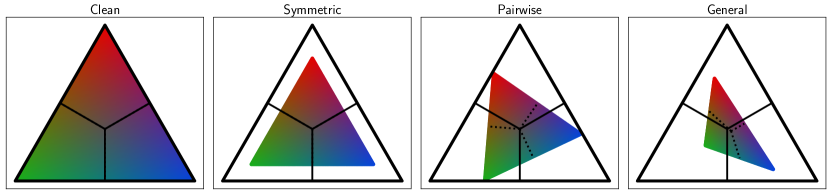
Figure 2: Illustrations of the noise transition matrix as a linear transformation $\Delta\to{\mathrm{Conv}}({\bm{T}})$ when $K=3$, including symmetric, pair flipping, and general noises. The outer black triangle is the simplex $\Delta$ and the inner colored triangle is the convex hull ${\mathrm{Conv}}({\bm{T}})$. Solid lines are the decision boundaries of argmax and dotted lines are the ones after the transformation. Note that different transition matrices affect the decision boundary differently. Adding symmetric noise does not change the decision boundary.

2 Problem: Class-Conditional Noise

In this section, we review the notation, assumption, and related work in learning with class-conditional noise (CCN).

2.1 Noisy Labels

Let $X\in{\mathcal{X}}$ be the input feature, and $Y\in\{1,\dots,K\}$ the true label, where $K$ is the number of classes. In fully supervised learning, we can fit a discriminative model for the conditional probability $p(Y|X)$ using an i.i.d. sample of $(X,Y)$-pairs. However, observed labels may be corrupted in many real-world applications. Treating the corrupted label as correct usually leads to poor performance (Arpit et al., 2017; Zhang et al., 2017). In this work, we explicitly model this label corruption process. We denote the noisy label by ${\widetilde{Y}}\in\{1,\dots,K\}$. The goal is to predict $Y$ from $X$ based on an i.i.d. sample of $(X,{\widetilde{Y}})$-pairs.

2.2 Class-Conditional Noise (CCN)

Next, we formulate the class-conditional noise (CCN) model (Natarajan et al., 2013; Patrini et al., 2017).

In CCN, we have the following assumption:

$$p({\widetilde{Y}}|Y,X)=p({\widetilde{Y}}|Y).$$ (1)

That is, the noisy label ${\widetilde{Y}}$ only depends on the true label $Y$ but not on $X$. Then, we can relate the noisy class-posterior $p({\widetilde{Y}}|X)$ and the clean class-posterior $p(Y|X)$ by

$$\textstyle p({\widetilde{Y}}|X)=\sum_{Y=1}^{K}p({\widetilde{Y}}|Y)p(Y|X).$$ (2)

Note that the clean class-posterior $p(Y|X)$ can be seen as a vector-valued function ${\bm{p}}(Y|X=x):{\mathcal{X}}\to\Delta^{K-1}\vcentcolon=[p(Y=1|X=x),\ldots,p(Y=K|X=x)]^{\mathsf{T}}$, and so can the noisy class-posterior $p({\widetilde{Y}}|X)$. Also, $p({\widetilde{Y}}|Y)$ can be written in matrix form: ${\bm{T}}\in{\mathcal{T}}\subset[0,1]^{K\times K}$ with elements ${\bm{T}}_{ij}=p({\widetilde{Y}}=j|Y=i)$ for $i,j\in\{1,\ldots,K\}$, where ${\mathcal{T}}$ is the set of all full-rank row stochastic matrices. Here, ${\bm{T}}$ is called a noise transition matrix. Then, with the vector and matrix notation, Eq. 2 can be rewritten as

$${\bm{p}}({\widetilde{Y}}|X)={\bm{T}}^{\mathsf{T}}{\bm{p}}(Y|X).$$ (3)

Note that multiplying ${\bm{T}}$ is a linear transformation from the simplex $\Delta$ to the convex hull ${\mathrm{Conv}}({\bm{T}})$ induced by rows of ${\bm{T}}$, which is illustrated in Fig. 2.

In the context of learning from noisy labels, we further assume ${\bm{T}}$ to be diagonally dominant in the sense that ${\bm{T}}_{ii}>{\bm{T}}_{ij}$ for $i\neq j$. Although this formulation can be also used for learning from complementary labels, where ${\bm{T}}_{ii}=0$ or ${\bm{T}}_{ii}<{\bm{T}}_{ij}$ for $i\neq j$ (Ishida et al., 2017; Yu et al., 2018).

2.3 Learning with Known Noise Transition Matrix

If the ground-truth noise transition matrix ${\bm{T}}$ is known, ${\bm{p}}(Y|X)$ is identifiable based on observations of ${\bm{p}}({\widetilde{Y}}|X)$, which means that different ${\bm{p}}(Y|X)$ must generate distinct ${\bm{p}}({\widetilde{Y}}|X)$. Therefore, we can consistently recover ${\bm{p}}(Y|X)$ by estimating ${\bm{p}}({\widetilde{Y}}|X)$ using the relation in Eq. 3 (Patrini et al., 2017; Yu et al., 2018). However, if ${\bm{T}}$ and ${\bm{p}}(Y|X)$ are both unknown, then they are both partially identifiable because there could be multiple observationally equivalent ${\bm{T}}$ and ${\bm{p}}(Y|X)$ whose product equals ${\bm{p}}({\widetilde{Y}}|X)$. Thus, it is impossible to estimate both ${\bm{T}}$ and ${\bm{p}}(Y|X)$ from ${\bm{p}}({\widetilde{Y}}|X)$ without any additional assumption.

Concretely, let ${\widehat{{\bm{p}}}}(Y|X;W)$ parameterized by $W\in{\mathcal{W}}$ be a differentiable model for the true label, and ${\widehat{{\bm{T}}}}\in{\mathcal{T}}$ be an estimator for the noise transition matrix. We consider a sufficiently large function class of ${\widehat{{\bm{p}}}}(Y|X;W)$ that contains the ground-truth ${\bm{p}}(Y|X)$, i.e., $\exists W^{*}\in{\mathcal{W}},{\widehat{{\bm{p}}}}(Y|X;W^{*})={\bm{p}}(Y|X)\textnormal{ a.e.}$ In practice, we use an expressive deep neural network (Goodfellow et al., 2016) as ${\widehat{{\bm{p}}}}(Y|X;W)$.

Then, let us consider the expected Kullback–Leibler (KL) divergence as the learning objective:

$$L_{0}(W,{\widehat{{\bm{T}}}})\vcentcolon=\operatorname*{\mathbb{E}}_{X\sim p(X)}\left[D_{\mathrm{KL}}\left({\bm{p}}({\widetilde{Y}}|X)\;\middle\|\;{\widehat{{\bm{T}}}}^{\mathsf{T}}{\widehat{{\bm{p}}}}(Y|X;W)\right)\right],$$ (4)

which is related to the expected negative log-likelihood or the cross-entropy loss in the following way:

$$L(W,{\widehat{{\bm{T}}}}) \vcentcolon=\operatorname*{\mathbb{E}}_{X,{\widetilde{Y}}\sim p(X,{\widetilde{Y}})}\left[-\log({\widehat{{\bm{T}}}}_{{\widetilde{Y}}}^{\mathsf{T}}{\widehat{{\bm{p}}}}(Y|X;W))\right]$$ (5)

$$=L_{0}(W,{\widehat{{\bm{T}}}})+H({\widetilde{Y}}|X),$$ (6)

where the second term $H({\widetilde{Y}}|X)$ is the conditional entropy of ${\widetilde{Y}}$ given $X$, which is a constant w.r.t. $W$ and ${\widehat{{\bm{T}}}}$. Note that $L(W,{\widehat{{\bm{T}}}})$ is minimized if and only if $L_{0}(W,{\widehat{{\bm{T}}}})=0$.

When $L(W,{\widehat{{\bm{T}}}})$ is empirically estimated and optimized based on a finite sample of $(X,{\widetilde{Y}})$-pairs, we can ensure that ${\widehat{{\bm{T}}}}^{\mathsf{T}}{\widehat{{\bm{p}}}}(Y|X){\xrightarrow{\mathrm{d}}}{\bm{T}}^{\mathsf{T}}{\bm{p}}(Y|X)$ as the sample size increases, but we can not guarantee that ${\widehat{{\bm{p}}}}(Y|X){\xrightarrow{\mathrm{d}}}{\bm{p}}(Y|X)$ due to non-identifiability. The latter holds only when the ground-truth ${\bm{T}}$ is used as ${\widehat{{\bm{T}}}}$ (Patrini et al., 2017).

2.4 Learning with Unknown Noise Transition Matrix

In real-world applications, the ground-truth ${\bm{T}}$ is usually unknown. Some existing two-step methods attempted to transform this problem to the previously solved one by first estimating the noise transition matrix and then using it in neural network training. Since it is rare to have both clean labels $Y$ and noisy labels ${\widetilde{Y}}$ for the same instance $X$, several methods are proposed to estimate ${\bm{T}}$ from only noisy data.

Existing methods usually rely on a separate set of anchor points (Liu & Tao, 2015; Patrini et al., 2017; Yu et al., 2018; Xia et al., 2019; Yao et al., 2020), which are defined as follows:

Definition 1 (Anchor point).

An instance $x$ is called an anchor point for class $i$ if $p(Y=i|X=x)=1$.

Based on an anchor point $x$ for class $i$, we have

$${\bm{p}}({\widetilde{Y}}|X=x)={\bm{T}}^{\mathsf{T}}{\bm{p}}(Y|X=x)={\bm{T}}_{i}.$$ (7)

Thus, we can first estimate ${\bm{p}}({\widetilde{Y}}|X)$ and then calculate the value on anchor points to obtain an estimate of ${\bm{T}}$. However, if we cannot find such anchor points in real-world datasets easily, the aforementioned method can not be applied.

A workaround is to detect anchor points from all noisy data, assuming that they exist in the dataset. Further revision of the transition matrix before (Yao et al., 2020) or during (Xia et al., 2019) the second stage of training can be adopted to improve the performance.

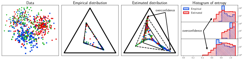
Figure 3: An example of overconfident predictions yield from neural networks. Notation: • Shape: true labels • Color: observed labels • Location in the simplex: ground-truth/estimated probabilities • Solid triangle: convex hull ${\mathrm{Conv}}({\bm{T}})$ • Dashed triangle: convex hull of an estimated transition matrix • Vertices of the triangle: anchor points . Without knowing ${\bm{T}}$ and the constraint that ${\bm{p}}({\widetilde{Y}}|X)$ should be within ${\mathrm{Conv}}({\bm{T}})$, a neural network trained with noisy labels tends to output high-confident (low-entropy) predictions outside of ${\mathrm{Conv}}({\bm{T}})$. Therefore, ${\bm{T}}$ may be poorly estimated based on the overconfident noisy class-posterior.

Nevertheless, such two-step methods based on anchor points face an inevitable problem — the estimation of the noisy class-posterior ${\bm{p}}({\widetilde{Y}}|X)$ using possibly over-parameterized neural networks trained with noisy labels. We point out that the estimation error could be high in this step because of the overconfidence problem of deep neural networks (Guo et al., 2017; Hein et al., 2019). If no revision is made, errors in the first stage may lead to major errors in the second stage.

Figure 3 illustrates an example of the overconfidence. As discussed in Section 2.2, ${\bm{p}}({\widetilde{Y}}|X)$ should be within the convex hull ${\mathrm{Conv}}({\bm{T}})$. However, without knowing ${\bm{T}}$ and this constraint, a neural network trained with noisy labels tends to output overconfident probabilities that are outside of ${\mathrm{Conv}}({\bm{T}})$. Note that over-parameterized neural networks trained with clean labels could also be overconfident and several re-calibration methods are developed to alleviate this issue (Guo et al., 2017; Kull et al., 2019; Hein et al., 2019; Rahimi et al., 2020). However, in Appendix B we demonstrate that estimating the noise class-posterior causes a significantly worse overconfidence issue than estimating the clean one. Consequently, transition matrix estimation may suffer from poorly estimated noisy class-posteriors, which leads to performance degradation.

In contrast to existing methods, our proposed method only uses the product ${\widehat{{\bm{T}}}}^{\mathsf{T}}{\widehat{{\bm{p}}}}(Y|X)$ as an estimate of ${\bm{p}}({\widetilde{Y}}|X)$ and never estimates ${\bm{p}}({\widetilde{Y}}|X)$ directly using neural networks.

3 Motivation

In this section, we take a closer look at the class-conditional label corruption process and construct an equivalence class and a partial order for the noise transition matrix, which motivates our proposed method. Concretely, we show that the contraction property of the stochastic matrices leads to a partial order of the transition matrices, which can be used to find the “cleanest” clean class-posterior.

3.1 Transition Matrix Equivalence

Recall that ${\mathcal{T}}$ is the set of full-rank row stochastic matrices, which is closed under multiplication. Based on this, we first define an equivalence relation of an ordered pair of transition matrices induced by the product:

Definition 2 (Transition matrix equivalence).

$$({\bm{U}},{\bm{V}})\sim({\bm{U}}^{\prime},{\bm{V}}^{\prime})\Leftrightarrow{\bm{U}}{\bm{V}}={\bm{U}}^{\prime}{\bm{V}}^{\prime}.$$

The corresponding equivalence class with a product ${\bm{W}}$ is denoted by $[{\bm{W}}]$. Specially, for the identity matrix ${\bm{I}}$, $[{\bm{I}}]$ contains pairs of permutation matrices $({\bm{P}},{\bm{P}}^{-1})$; for a non-identity matrix ${\bm{W}}$, $[{\bm{W}}]$ contains at least two distinct elements $({\bm{W}},{\bm{I}})$ and $({\bm{I}},{\bm{W}})$ and possibly infinitely many other elements.

Now, consider the equivalence class $[{\bm{T}}]$ for the ground-truth noise transition matrix ${\bm{T}}$ in our problem. Then, any element $({\bm{U}},{\bm{V}})\in[{\bm{T}}]$ corresponds to a possible optimal solution of Eq. 5: ${\widehat{{\bm{T}}}}={\bm{V}}$ and ${\widehat{{\bm{p}}}}(Y|X;W)={\bm{U}}^{\mathsf{T}}{\bm{p}}(Y|X)$, given that such a parameter $W$ exists. Among possibly infinitely many possibilities, only $({\bm{I}},{\bm{T}})$ is of our central interest. However, it is possible to get infinitely many other wrong ones, such as $({\bm{T}},{\bm{I}})$, which corresponds to a model that predicts the noisy class-posterior and chooses the transition matrix to be the identity matrix ${\bm{I}}$.

3.2 Transition Matrix Decomposition

Next, consider the reverse direction: if we obtain an optimal solution of Eq. 5, ${\widehat{{\bm{T}}}}$ and ${\widehat{{\bm{p}}}}(Y|X)$, is there a ${\bm{U}}$ such that ${\widehat{{\bm{p}}}}(Y|X)={\bm{U}}^{\mathsf{T}}{\bm{p}}(Y|X)$? The answer is yes if there are anchor points for each class in the dataset, which can be proved using the following theorem: [Transition matrix decomposition] For two row stochastic matrices ${\bm{W}},{\bm{V}}\in{\mathcal{T}}$, if $\forall{\bm{p}}\in\Delta$, $\exists{\bm{q}}\in\Delta$, s.t. ${\bm{W}}^{\mathsf{T}}{\bm{p}}={\bm{V}}^{\mathsf{T}}{\bm{q}}$, then $\exists$ a row stochastic matrix ${\bm{U}}\in{\mathcal{T}}$, s.t. ${\bm{W}}={\bm{U}}{\bm{V}}$ and $\forall{\bm{p}}\in\Delta$, ${\bm{q}}={\bm{U}}^{\mathsf{T}}{\bm{p}}$.

Proof.

Let ${\bm{p}}$ be ${\bm{e}}_{i}$ and denote the corresponding ${\bm{q}}$ by ${\bm{q}}_{i}$ for $i=1,\dots,K$. Then ${\bm{U}}=[{\bm{q}}_{1},\dots,{\bm{q}}_{K}]^{\mathsf{T}}$. ∎

Here, ${\bm{e}}_{i}$ is the $i$-th standard basis and ${\bm{p}}(Y|X=x)={\bm{e}}_{i}$ means that $x$ is an anchor point for the class $i$. Consequently, we can derive that if there are anchor points for each class in the dataset, given an estimated transition matrix ${\widehat{{\bm{T}}}}$ and an estimated clean class-posterior ${\widehat{{\bm{p}}}}(Y|X)$ from an optimal solution of Eq. 5, we know that there is an implicit row stochastic matrix ${\bm{U}}$ such that ${\widehat{{\bm{p}}}}(Y|X)={\bm{U}}^{\mathsf{T}}{\bm{p}}(Y|X)$. In other words, the estimate ${\widehat{{\bm{p}}}}(Y|X)$ may still contain class-conditional label noise, which is described by ${\bm{U}}$.

We point out that the existence of anchor points is a sufficient but not necessary condition for the existence of the ${\bm{U}}$ above. If anchor points do not exist, we may or may not find such a ${\bm{U}}$. Also note that we will not try to detect anchor points from noisy data.

More importantly, we have no intention of estimating ${\bm{U}}$ explicitly. In this work, we only use the fact that there is a one-to-one correspondence between optimal solutions of Eq. 5 and elements in the equivalence class $[{\bm{T}}]$ under the above assumption. Based on this fact, we can study the equivalence class $[{\bm{T}}]$ or the properties of the implicit ${\bm{U}}$ instead, which is easier to deal with.

3.3 Transition Matrix as a Contraction Mapping

Next, we attempt to break the equivalence introduced above by examining the characteristics of this consecutive class-conditional label corruption process.

We start with the definition of the total variation distance $d_{\mathrm{TV}}(\cdot,\cdot)$ between pairs of categorical probabilities:

$$d_{\mathrm{TV}}({\bm{p}},{\bm{q}})\vcentcolon=\frac{1}{2}\lVert{\bm{p}}-{\bm{q}}\rVert_{1},$$ (8)

where $\lVert\cdot\rVert_{1}$ denotes the $\ell_{1}$ norm. Then, from the theory of Markov chains, we know that the mapping $\Delta\to{\mathrm{Conv}}({\bm{U}})$ defined by ${\bm{p}}\mapsto{\bm{U}}^{\mathsf{T}}{\bm{p}}$ is a contraction mapping over the simplex $\Delta$ relative to the total variation distance (Del Moral et al., 2003), which means that $\forall{\bm{U}}\in{\mathcal{T}},\forall{\bm{p}},{\bm{q}}\in\Delta$,

$$d_{\mathrm{TV}}({\bm{U}}^{\mathsf{T}}{\bm{p}},{\bm{U}}^{\mathsf{T}}{\bm{q}})\leq d_{\mathrm{TV}}({\bm{p}},{\bm{q}}).$$ (9)

3.4 Transition Matrix Partial Order

Finally, based on this contraction property of the stochastic matrices, we can introduce a partial order induced by the total variation distance within the equivalence class $[{\bm{T}}]$:

Definition 3 (Transition matrix partial order).

$$({\bm{U}},{\bm{V}})\preceq({\bm{U}}^{\prime},{\bm{V}}^{\prime})\Leftrightarrow$$

$$\forall{\bm{p}},{\bm{q}}\in\Delta,d_{\mathrm{TV}}({\bm{U}}^{\mathsf{T}}{\bm{p}},{\bm{U}}^{\mathsf{T}}{\bm{q}})\leq d_{\mathrm{TV}}({\bm{U}}^{\prime\mathsf{T}}{\bm{p}},{\bm{U}}^{\prime\mathsf{T}}{\bm{q}}).$$

Note that $({\bm{I}},{\bm{T}})$ is the unique greatest element because of Eq. 9. Despite the fact that there could be incomparable elements, we may gradually increase the total variation to find $({\bm{I}},{\bm{T}})$. Then, with the help of this partial order, it is possible to estimate both ${\bm{p}}(Y|X)$ and ${\bm{T}}$ simultaneously, which is discussed in the following section.

4 Proposed Method

In this section, we present our proposed method. Overall, the proposed method is illustrated in Fig. 1.

Summarizing our motivation discussed in Section 3, we found that if anchor points exist in the dataset, estimating both the transition matrix ${\bm{T}}$ and the clean class-posterior ${\bm{p}}(Y|X)$ by training with the cross-entropy loss in Eq. 5 results in a solution in the form ${\widehat{{\bm{p}}}}(Y|X)={\bm{U}}^{\mathsf{T}}{\bm{p}}(Y|X)$, where ${\bm{U}}$ is an unknown transition matrix (Section 3.2). Then, we pointed out that the stochastic matrices have the contraction property shown in Eq. 9 so that the “cleanest” clean class-posterior has the highest pairwise total variation defined in Eq. 8. Based on this fact, we can regularize the predicted probabilities to be more distinguishable from each other to find the optimal solution, as discussed below.

4.1 Total Variation Regularization

First, we discuss how to enforce our preference of more distinguishable predictions in terms of the total variation distance. We start with defining the expected pairwise total variation distance:

$$R(W) \vcentcolon=\operatorname*{\mathbb{E}}_{x_{1}\sim p(X)}\operatorname*{\mathbb{E}}_{x_{2}\sim p(X)}[d_{\mathrm{TV}}({\widehat{{\bm{p}}}}_{1},{\widehat{{\bm{p}}}}_{2})],$$ (10)

$$\textnormal{ where }{\widehat{{\bm{p}}}}_{i} \vcentcolon={\widehat{{\bm{p}}}}(Y|X=x_{i};W),\quad i=1,2.$$

Note that this data-dependent term depends on $X$ but not on $Y$ nor on ${\widetilde{Y}}$.

Then, we adopt the learning objective in the KL-divergence form in Eq. 4, combine it with the expected pairwise total variation distance in Eq. 10, and formulate our approach in the form of constrained optimization, as stated in the following theorem: [Consistency] Given a finite i.i.d. sample of $(X,{\widetilde{Y}})$-pairs of size $N$, where anchor points (Definition 1) for each class exist in the sample, let ${\widetilde{L}}_{0}(W,{\widehat{{\bm{T}}}})$ and ${\widetilde{R}}(W)$ be the empirical estimates of $L_{0}(W,{\widehat{{\bm{T}}}})$ in Eq. 4 and $R(W)$ in Eq. 10, respectively. Assume that the parameter space ${\mathcal{W}}$ is compact. Let $(W^{\circ},{\widehat{{\bm{T}}}}^{\circ})$ be an optimal solution of the following constrained optimization problem:

$$\max_{W}{\widetilde{R}}(W)\textnormal{ s.t. }{\widetilde{L}}_{0}(W,{\widehat{{\bm{T}}}})=0.$$ (11)

Then, ${\widehat{{\bm{T}}}}^{\circ}$ is a consistent estimator of the transition matrix ${\bm{T}}$; and ${\widehat{{\bm{p}}}}(Y|X;W^{\circ}){\xrightarrow{\mathrm{d}}}{\bm{p}}(Y|X)\textnormal{ a.e.}$ as $N\to\infty$. The proof is given in Appendix C. Informally, we make use of Section 3.2, the property of the KL-divergence, and the contraction property of the transition matrix.

In practice, the constrained optimization in Eq. 11 can be solved via the following Lagrangian (Kuhn et al., 1951):

$$\mathcal{L}(W,{\widehat{{\bm{T}}}})\vcentcolon={\widetilde{L}}_{0}(W,{\widehat{{\bm{T}}}})-\gamma{\widetilde{R}}(W),$$ (12)

where $\gamma\in{\mathbb{R}}_{>0}$ is a parameter controlling the importance of the regularization term. We call such a regularization term a total variation regularization. This Lagrangian technique has been widely used in the literature (Cortes & Vapnik, 1995; Kloft et al., 2009; Higgins et al., 2017; Li et al., 2021). When the total variation regularization term is empirically estimated and optimized, we can sample a fixed number of pairs to reduce the additional computational cost.

4.2 Transition Matrix Estimation

Next, we discuss the estimation of the transition matrix ${\bm{T}}$. In contrast to existing methods (Patrini et al., 2017; Xia et al., 2019; Yao et al., 2020), we adopt a one-step training procedure to obtain both ${\widehat{{\bm{p}}}}(Y|X)$ and ${\widehat{{\bm{T}}}}$ simultaneously.

Gradient-based estimation.

First, note that the learning objective Eq. 12 is differentiable w.r.t. ${\widehat{{\bm{T}}}}$. As a baseline, it is sufficient to use gradient-based optimization for ${\widehat{{\bm{T}}}}$. In practice, we apply softmax to an unconstrained matrix in ${\mathbb{R}}^{K\times K}$ to ensure that ${\widehat{{\bm{T}}}}\in{\mathcal{T}}$. Then, ${\widehat{{\bm{T}}}}$ is estimated by optimizing $\mathcal{L}(W,{\widehat{{\bm{T}}}})$ using stochastic gradient descent (SGD) or its variants (e.g., Kingma & Ba (2015)).

Dirichlet posterior update.

The additional total variation regularization term Eq. 10 is irrelevant to ${\widehat{{\bm{T}}}}$ so we are free to use other optimization methods besides gradient-based methods. To capture the uncertainty of the estimation of ${\bm{T}}$ during different stages of training, we propose an alternative derivative-free approach that uses Dirichlet distributions to model ${\bm{T}}$. Concretely, let the posterior of ${\bm{T}}$ be

$$\widehat{{\bm{T}}}_{i}\sim\mathrm{Dirichlet}({\bm{A}}_{i})\quad(i=1,\dots,K),$$ (13)

where ${\bm{A}}_{i}\in{\mathbb{R}}_{>0}^{K}$ is the concentration parameter. Denote the confusion matrix by ${\bm{C}}\in{\mathbb{N}}_{\geq 0}^{K\times K}$, where its element ${\bm{C}}_{ij}$ is the number of instances that are predicted to be ${\widehat{Y}}=i$ via sampling ${\widehat{Y}}\sim{\widehat{{\bm{p}}}}(Y|X;W)$ but are labeled as ${\widetilde{Y}}=j$ in the noisy dataset. In other words, we use a posterior of $p({\widetilde{Y}}|{\widehat{Y}})$ to approximate $p({\widetilde{Y}}|Y)$ during training.

Then, inspired by the closed-form posterior update rule for the Dirichlet-multinomial conjugate (Diaconis & Ylvisaker, 1979):

$${\bm{A}}^{(\mathrm{posterior})}={\bm{A}}^{(\mathrm{prior})}+{\bm{C}}^{(\mathrm{observation})},$$ (14)

we update the concentration parameters ${\bm{A}}$ during training using the confusion matrix ${\bm{C}}$ via the following update rule:

$${\bm{A}}\leftarrow\beta_{1}{\bm{A}}+\beta_{2}{\bm{C}},$$ (15)

where ${\bm{\beta}}=(\beta_{1},\beta_{2})$ are fixed hyperparameters that control the convergence of ${\bm{A}}$. We initialize ${\bm{A}}$ with an appropriate diagonally dominant matrix to reflect our prior knowledge of noisy labels. For each batch of data, we sample a noise transition matrix $\widehat{{\bm{T}}}$ from the Dirichlet posterior and use it in our learning objective in Eq. 12.

The idea is that the confusion matrix ${\bm{C}}$ at any stage during training is a crude estimator of the true noise transition matrix ${\bm{T}}$, then we can improve this estimator based on information obtained during training. Because at earlier stage of training, this estimator is very crude and may be deviated from the true one significantly, we use a decaying factor $\beta_{1}$ close to $1$ (e.g., $0.999$) to let the model gradually “forget” earlier information. Meanwhile, $\beta_{2}$ controls the variance of the Dirichlet posterior during training, which is related to the learning rate and batch size. At early stages, the variance is high so the model is free to explore various transition matrices; as the model converges, the estimation of the transition matrix also becomes more precise so the posterior would concentrate around the true one.

Table 1: Accuracy ($\%$) on the MNIST, CIFAR-10, and CIFAR-100 datasets. We reported “mean (standard deviation)” of $10$ trials.

		(a) Clean	(b) Symm.	(c) Pair	(d) Pair2	(e) Trid.	(f) Rand.
MNIST	MAE	$98.72(0.09)$	$98.00(0.14)$	$91.46(7.40)$	$89.79(6.11)$	$96.22(3.87)$	$34.07(31.98)$
	CCE	$\mathbf{99.21(0.04)}$	$98.13(0.16)$	$94.70(0.64)$	$94.86(0.67)$	$96.78(0.22)$	$95.68(1.31)$
	GCE	$99.12(0.06)$	$98.41(0.12)$	$93.79(1.04)$	$94.06(0.63)$	$96.60(0.14)$	$96.28(0.93)$
	Forward	$\mathbf{99.18(0.05)}$	$98.00(0.24)$	$94.37(1.00)$	$94.84(0.53)$	$96.54(0.29)$	$95.95(1.49)$
	T-Revision	$\mathbf{99.20(0.06)}$	$98.01(0.14)$	$94.19(0.78)$	$95.24(0.74)$	$96.76(0.15)$	$96.62(0.70)$
	Dual-T	$99.16(0.05)$	$\mathbf{98.58(0.12)}$	$\mathbf{99.06(0.07)}$	$\mathbf{99.03(0.06)}$	$\mathbf{99.04(0.05)}$	$\mathbf{98.79(0.17)}$
	TVG	$99.16(0.06)$	$\mathbf{98.55(0.09)}$	$94.26(0.59)$	$95.42(0.44)$	$97.78(0.56)$	$97.67(0.84)$
	TVD	$\mathbf{99.18(0.07)}$	$\mathbf{98.56(0.08)}$	$\mathbf{99.09(0.08)}$	$\mathbf{99.00(0.07)}$	$\mathbf{99.03(0.08)}$	$\mathbf{98.82(0.11)}$
CIFAR10	MAE	$66.47(4.76)$	$57.23(4.15)$	$44.29(2.23)$	$42.43(1.66)$	$43.43(2.69)$	$26.95(5.45)$
	CCE	$\mathbf{91.87(0.19)}$	$75.71(0.57)$	$65.54(0.66)$	$65.23(0.85)$	$76.07(0.61)$	$70.44(1.98)$
	GCE	$89.25(0.17)$	$\mathbf{83.68(0.29)}$	$71.49(1.18)$	$69.66(0.57)$	$82.14(0.41)$	$78.07(2.16)$
	Forward	$\mathbf{91.87(0.15)}$	$76.18(0.63)$	$65.42(0.92)$	$65.65(1.11)$	$76.41(0.50)$	$70.86(2.19)$
	T-Revision	$91.72(0.18)$	$75.51(0.59)$	$65.49(0.97)$	$65.70(0.66)$	$76.18(0.80)$	$71.22(1.62)$
	Dual-T	$\mathbf{91.75(0.18)}$	$82.85(0.42)$	$80.86(1.03)$	$79.61(1.20)$	$\mathbf{88.11(0.28)}$	$84.33(2.11)$
	TVG	$91.61(0.14)$	$82.60(0.38)$	$\mathbf{89.78(0.16)}$	$\mathbf{88.36(0.24)}$	$\mathbf{88.07(0.25)}$	$\mathbf{86.19(0.52)}$
	TVD	$91.00(0.13)$	$83.03(0.24)$	$88.47(0.29)$	$86.96(0.35)$	$87.44(0.16)$	$\mathbf{85.86(0.46)}$
CIFAR100	MAE	$11.23(1.02)$	$7.89(0.67)$	$6.94(1.11)$	$6.60(0.74)$	$7.45(0.55)$	$7.15(0.98)$
	CCE	$\mathbf{70.58(0.29)}$	$42.94(0.47)$	$44.00(0.71)$	$41.37(0.27)$	$46.55(0.54)$	$42.41(0.48)$
	GCE	$57.10(0.85)$	$48.66(0.58)$	$45.27(0.85)$	$43.67(0.94)$	$50.98(0.33)$	$48.66(0.63)$
	Forward	$\mathbf{70.58(0.28)}$	$44.32(0.64)$	$44.17(0.57)$	$42.07(0.55)$	$47.48(0.40)$	$43.15(0.53)$
	T-Revision	$\mathbf{70.47(0.26)}$	$46.52(0.57)$	$44.08(0.42)$	$42.01(0.52)$	$47.59(0.60)$	$45.33(0.40)$
	Dual-T	$\mathbf{70.56(0.28)}$	$55.92(0.60)$	$46.22(0.72)$	$44.74(0.65)$	$61.68(0.51)$	$57.92(0.50)$
	TVG	$70.02(0.30)$	$\mathbf{57.33(0.42)}$	$45.68(0.85)$	$44.38(0.72)$	$54.23(0.53)$	$\mathbf{59.85(0.61)}$
	TVD	$69.93(0.21)$	$52.54(0.45)$	$\mathbf{56.02(0.82)}$	$\mathbf{49.18(0.53)}$	$\mathbf{62.45(0.44)}$	$53.95(0.47)$

Table 2: Average total variation ($\times 100$) on the MNIST, CIFAR-10, and CIFAR-100 datasets. We reported “mean (standard deviation)” of $10$ trials.

		(a) Clean	(b) Symm.	(c) Pair	(d) Pair2	(e) Trid.	(f) Rand.
MNIST	Forward	$\mathbf{0.00(0.00)}$	$34.14(3.03)$	$39.71(0.15)$	$41.98(0.82)$	$38.33(0.93)$	$30.45(2.16)$
	T-Revision	$0.03(0.02)$	$32.94(3.22)$	$39.87(0.08)$	$41.50(0.50)$	$38.39(1.34)$	$29.35(1.85)$
	Dual-T	$0.12(0.02)$	$7.12(0.99)$	$3.90(0.66)$	$3.59(0.58)$	$3.11(0.88)$	$10.63(0.90)$
	TVG	$2.36(0.01)$	$\mathbf{1.47(0.13)}$	$39.29(0.03)$	$32.17(0.93)$	$14.11(5.21)$	$7.33(4.25)$
	TVD	$2.06(0.12)$	$1.96(0.17)$	$\mathbf{2.12(0.21)}$	$\mathbf{2.12(0.10)}$	$\mathbf{1.92(0.11)}$	$\mathbf{2.13(0.22)}$
CIFAR-10	Forward	$\mathbf{0.00(0.00)}$	$47.63(0.35)$	$39.09(0.28)$	$41.70(0.32)$	$35.63(0.81)$	$45.52(0.65)$
	T-Revision	$0.03(0.03)$	$43.05(0.36)$	$39.13(0.22)$	$40.80(0.30)$	$34.82(0.67)$	$43.05(0.52)$
	Dual-T	$0.81(0.04)$	$\mathbf{2.99(0.23)}$	$19.37(0.45)$	$16.84(0.61)$	$4.60(0.31)$	$8.80(1.57)$
	TVG	$0.64(0.01)$	$3.17(0.19)$	$\mathbf{1.56(0.13)}$	$\mathbf{2.16(0.22)}$	$\mathbf{1.94(0.18)}$	$\mathbf{2.24(0.26)}$
	TVD	$7.87(0.10)$	$6.90(0.18)$	$8.46(0.17)$	$8.70(0.24)$	$7.06(0.14)$	$7.98(0.38)$
CIFAR-100	Forward	$\mathbf{0.00(0.00)}$	$48.62(0.11)$	$39.81(0.03)$	$43.57(0.04)$	$40.92(0.07)$	$49.06(0.10)$
	T-Revision	$0.46(0.05)$	$31.58(0.46)$	$39.45(0.03)$	$42.77(0.06)$	$40.01(0.09)$	$39.49(0.26)$
	Dual-T	$3.10(0.08)$	$17.10(0.18)$	$33.26(0.20)$	$33.79(0.26)$	$\mathbf{23.56(0.43)}$	$22.59(0.23)$
	TVG	$1.59(0.02)$	$\mathbf{13.11(0.10)}$	$37.79(0.30)$	$38.83(0.34)$	$30.80(0.51)$	$\mathbf{16.47(0.18)}$
	TVD	$21.98(0.11)$	$26.46(0.15)$	$\mathbf{29.47(0.26)}$	$\mathbf{31.34(0.30)}$	$23.86(0.22)$	$35.37(0.30)$

5 Related Work

In addition to methods using the noise transition matrix explicitly and two-step methods detecting anchor points from noisy data (Patrini et al., 2017; Yu et al., 2018; Xia et al., 2019; Yao et al., 2020) introduced in Sections 1 and 2, in this section we review related work in learning from noisy labels in a broader sense.

First, in CCN, is it possible to learn a correct classifier without the noise transition matrix? Existing studies in robust loss functions (Ghosh et al., 2017; Zhang & Sabuncu, 2018; Wang et al., 2019; Charoenphakdee et al., 2019; Ma et al., 2020; Feng et al., 2020; Lyu & Tsang, 2020; Liu & Guo, 2020) showed that it is possible to alleviate the label noise issue even without estimating the noise rate/transition matrix, under various conditions such as the noise being symmetric (the RCN model in binary classification (Angluin & Laird, 1988)). Further, it is proven that the accuracy metric itself can be robust (Chen et al., 2021). However, if the noise is heavy and complex, robust losses may perform poorly. This motivates us to evaluate our method under various types of label noises beyond the symmetric noise.

Another direction is to learn a classifier that is robust against label noise, including training sample selection (Malach & Shalev-Shwartz, 2017; Jiang et al., 2018; Han et al., 2018b; Wang et al., 2018; Yu et al., 2019; Wei et al., 2020; Mirzasoleiman et al., 2020; Wu et al., 2020) that selects training examples during training, learning with rejection (El-Yaniv & Wiener, 2010; Thulasidasan et al., 2019; Mozannar & Sontag, 2020; Charoenphakdee et al., 2021) that abstains from using confusing instances, meta-learning (Shu et al., 2019; Li et al., 2019), and semi-supervised learning (Nguyen et al., 2020; Li et al., 2020). These methods exploit the training dynamics, characteristics of loss distribution, or information of data itself instead of the class-posteriors. Then, the CCN assumption in Eq. 1 might not be needed but accordingly these methods usually have limited consistency guarantees. Moreover, the computational cost and model complexity of these methods could be higher.

For the CCN model and noise transition matrix estimation, recently, the idea of solving the class-conditional label noise problem using a one-step method was concurrently used by Li et al. (2021), aiming to relax the anchor point assumption. They adopt a different approach based on the characteristics of the noise transition matrix, instead of the properties of the clean class-posterior used in our work. Li et al. (2021) has the advantage that their assumption is weaker than ours. However, the additional term on the transition matrix might be incompatible with derivative-free optimization, such as the Dirichlet posterior update method proposed in our work.

6 Experiments

In this section, we present experimental results to show that the proposed method achieves lower estimation error of the transition matrix and consequently better classification accuracy for the true labels, confirming Section 4.1.

6.1 Benchmark Datasets

We evaluated our method on three image classification datasets, namely MNIST (LeCun et al., 1998), CIFAR-10, and CIFAR-100 (Krizhevsky, 2009). We used various noise types besides the common symmetric noise and pair flipping noise.

Concretely, noise types include: (a) (Clean) no additional synthetic noise, which serves as a baseline for the dataset and model (b) (Symm.) symmetric noise $50\%$ (Patrini et al., 2017) (c) (Pair) pair flipping noise $40\%$ (Han et al., 2018b) (d) (Pair²) a product of two pair flipping noise matrices with noise rates $30\%$ and $20\%$. Because the multiplication of pair flipping noise matrices is commutative, it is guaranteed to have multiple ways of decomposition of the transition matrix (e) (Trid.) tridiagonal noise (see also Han et al., 2018a), which corresponds to a spectral of classes where adjacent classes are easier to be mutually mislabeled, unlike the unidirectional pair flipping (f) (Rand.) random noise constructed by sampling a Dirichlet distribution and mixing with the identity matrix to a specified noise rate . See Appendix E for details.

Methods.

We compared the following methods: (1) (MAE) mean absolute error (Ghosh et al., 2017) as a robust loss (2) (CCE) categorical cross-entropy loss (3) (GCE) generalized cross-entropy loss (Zhang & Sabuncu, 2018) (4) (Forward) forward correction (Patrini et al., 2017) based on anchor points detection (5) (T-Revision) transition-revision (Xia et al., 2019) where the transition matrix is further revised during the second stage of training (6) (Dual-T) dual-T estimator (Yao et al., 2020) that uses the normalized confusion matrix to correct the transition matrix (7) (TVG) total variation regularization with the gradient-based estimation of ${\bm{T}}$ (8) (TVD) the one with the Dirichlet posterior update .

Models.

For MNIST, we used a sequential convolutional neural network (CNN) and an Adam optimizer (Kingma & Ba, 2015). For both CIFAR-10 and CIFAR-100, we used a residual network model ResNet-18 (He et al., 2016) and a stochastic gradient descent (SGD) optimizer with momentum (Sutskever et al., 2013).

Hyperparameters.

For the gradient-based estimation, we initialized the unconstrained matrix with diagonal elements of $\log(0.5)$ and off-diagonal elements of $\log(0.5/(K-1))$, so after applying softmax the diagonal elements are $0.5$. For the Dirichlet posterior update method, we initialized the concentration matrix with diagonal elements of $10$ for MNIST and $100$ otherwise and off-diagonal elements of $0$. We set ${\bm{\beta}}=(0.999,0.01)$ and $\gamma=0.1$. We sampled $512$ (the same as the batch size) pairs in each batch to calculate the pairwise total variation distance. Other hyperparameters are provided in Appendix E.

Evaluation metrics.

In addition to the test accuracy, we reported the average total variation to evaluate the transition matrix estimation, which is defined as follows:

$$\frac{1}{K}\sum_{i=1}^{K}d_{\mathrm{TV}}({\bm{T}}_{i},{\widehat{{\bm{T}}}}_{i})=\frac{1}{K}\sum_{i=1}^{K}\frac{1}{2}\sum_{j=1}^{K}\left\lvert{\bm{T}}_{ij}-{\widehat{{\bm{T}}}}_{ij}\right\rvert\in[0,1].$$

Results.

We ran $10$ trials for each experimental setting and reported “mean (standard deviation)” of the accuracy and average total variation in Tables 1 and 2, respectively. Outperforming methods are highlighted in boldface using one-tailed t-tests with a significance level of $0.05$.

In Table 1, we observed that the proposed methods performs well in terms of accuracy. Note that a baseline method Dual-T also showed superiority in some settings, which sheds light on the benefits of using the confusion matrix. However, as a two-step method, their computational cost is at least twice ours. In Table 2, we can confirm that in most settings, our methods have lower estimation error of the transition matrix than baselines, sometimes by a large margin. For better reusability, we fixed the initial transition matrix/concentration parameters across all different noise types. If we have more prior knowledge about the noise, a better initialization may further improve the performance.

Table 3: Accuracy ($\%$) on the Clothing1M dataset.

CCE	Forward	T-Revision	Dual-T	TVD
$69.91$	$69.96$	$69.97$	$70.67$	$71.65$

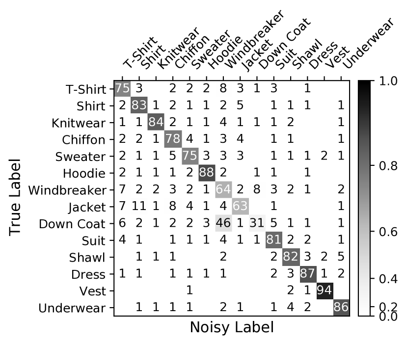
Figure 4: Estimated transition matrix ($\times 100$) on Clothing1M.

6.2 Real-World Dataset

We also evaluated our method on a real-world noisy label dataset, Clothing1M (Xiao et al., 2015). Unlike some previous work that also used a small set of clean training data (Patrini et al., 2017; Xia et al., 2019), we only used the $1M$ noisy training data. We followed previous work for other settings such as the model and optimization. We implemented data-parallel distributed training on $64$ NVIDIA Tesla P100 GPUs by PyTorch (Paszke et al., 2019). See Appendix E for details.

Results.

In Table 3, we reported the test accuracy. The transition matrix estimated by our proposed method was plotted in Fig. 4.

We can see that our method outperformed the baselines in terms of accuracy, which demonstrated the effectiveness of our method in real-world settings. Although there is no ground-truth transition matrix for evaluation, we can observe the similarity relationship between categories from the estimated transition matrix, which itself could be of great interest. For example, if two categories are relatively easy to be mutually mislabeled, they may be visually similar; if one category can be mislabeled as another, but not vice versa, we may get a semantically meaningful hierarchy of categories. Further investigation is left for future work.

7 Conclusion

We have introduced a novel method for estimating the noise transition matrix and learning a classifier simultaneously, given only noisy data. In this problem, the supervision is insufficient to identify the true model, i.e., we have a class of observationally equivalent models. We address this issue by finding characteristics of the true model under realistic assumptions and introducing a partial order as a regularization. As a result, the proposed total variation regularization is theoretically guaranteed to find the optimal transition matrix under mild conditions, which is reflected in experimental results on benchmark datasets.

Appendix A Beyond Class-Conditional Noise

In this section, we provide an overview of several selected noise models.

As introduced in Section 1, early studies focused on the most simple case — the random classification noise (RCN) model for binary classification (Angluin & Laird, 1988; Long & Servedio, 2010; Van Rooyen et al., 2015), where binary labels are flipped independently with a fixed noise rate $\displaystyle\rho\in[0,0.5)$. Here, $\displaystyle Y,{\widetilde{Y}}\in\{\pm 1\}$ and $\displaystyle\rho=p({\widetilde{Y}}=-1|Y=+1)=p({\widetilde{Y}}=-1|Y=+1)$. Then, still for binary classification, the class-conditional noise (CCN) model (Natarajan et al., 2013) extended the RCN model to the case where the noise rate depends on the class: $\displaystyle\rho_{+1}=p({\widetilde{Y}}=-1|Y=+1)$, $\displaystyle\rho_{-1}=p({\widetilde{Y}}=+1|Y=-1)$, $\displaystyle\rho_{+1}+\rho_{-1}<1$. These noise models are special cases of the multiclass CCN model (Patrini et al., 2017; Goldberger & Ben-Reuven, 2017; Han et al., 2018a; Xia et al., 2019; Yao et al., 2020), which is the main focus of our work.

A more general framework for learning with label noise is the mutual contamination (MC) model (Scott et al., 2013; Blanchard & Scott, 2014; du Plessis et al., 2014; Menon et al., 2015; Lu et al., 2019), where examples of each class are drawn separately. That is, $\displaystyle p(X|Y)$ is corrupted but not $\displaystyle p(Y|X)$. Consequently, the marginal distribution of data may not match the true marginal distribution. It is known that CCN is a special case of MC (Menon et al., 2015). For the binary case, there is a related problem of the transition matrix estimation, called mixture proportion estimation (MPE) (du Plessis et al., 2014; Scott, 2015; Ramaswamy et al., 2016), which has more technical difficulties. Our method may not work well in the MC setting because it explicitly relies on the i.i.d. assumption.

Further, the instance-dependent noise (IDN) model (Menon et al., 2018; Cheng et al., 2020; Berthon et al., 2021) has been assessed to only a limited extent but is of great interest recently. IDN still explicitly models the label corruption process as CCN bu removes the CCN assumption in Eq. 1. Therefore, the noise transition matrix could be instance-dependent and thus harder to estimate. In other words, $\displaystyle{\bm{T}}$ is not a fixed matrix anymore but a matrix-valued function of the instance $\displaystyle{\bm{T}}(X):{\mathcal{X}}\to{\mathcal{T}}$. Owing to its complexity, IDN has not been investigated extensively.

One simple way is to estimate the matrix-valued function $\displaystyle{\bm{T}}(X)$ and the clean class-posterior $\displaystyle p(Y|X)$ directly, assuming a certain level of smoothness of $\displaystyle{\bm{T}}(X)$ (Goldberger & Ben-Reuven, 2017). However, there is no theoretical guarantee and the estimation error could be very high. Another direction is to restrict the problem so we could provide some theoretical guarantees under certain conditions (Menon et al., 2018; Cheng et al., 2020). It is also a promising way to approximate IDN using a simpler dependency structure (Xiao et al., 2015; Xia et al., 2020), which works well in practice. Our method may also serve as a practical approximation of IDN without theoretical guarantee, which is reflected in the experiment on the Clothing1M dataset (Section 6). The use of regularization techniques in our work may inspire practical algorithm design for IDN.

Learning from noisy labels has a rich literature and there are several other noise models, e.g., capturing the uncertainty of labels without explicitly modeling the label corruption process. Although they are out of scope of our discussion.

Appendix B Overconfidence in Neural Networks

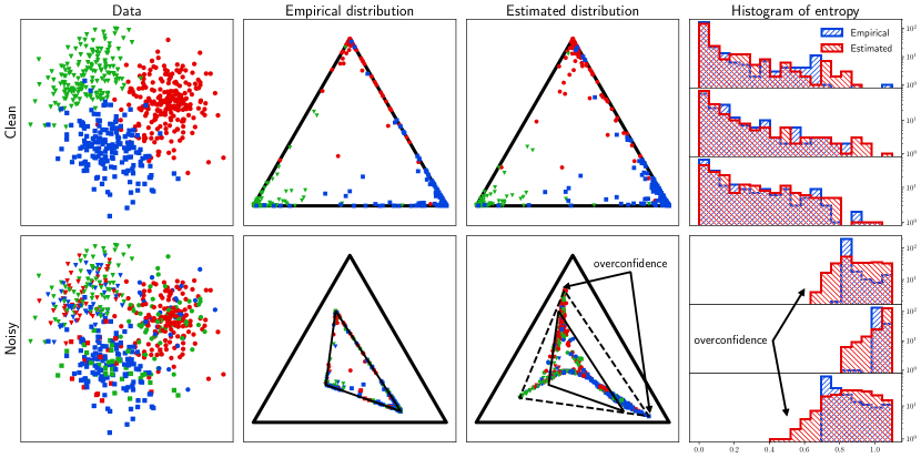
Figure 5: An example of overconfident predictions yield from neural networks, comparing the clean/noisy class-posterior estimation. See Fig. 3 for the notation.

In this section, we discuss the overconfidence phenomenon in neural networks, which is partially presented in Section 2.4.

In neural network training, if we only care the classification accuracy, the overconfidence is not a problem. We could use any classification-calibrated loss (Bartlett et al., 2006; Tewari & Bartlett, 2007), which only guarantees that the accuracy (0-1 risk) is asymptotically optimal. The class-posterior might not be recovered from the output of the classifier.

However, the transition matrix estimation based on anchor points (Patrini et al., 2017; Xia et al., 2019) — the method shown in Section 2.4 — heavily relies on a confidence-calibrated estimation of the noisy class-posterior using neural networks. The overconfidence issue of possibly over-parameterized neural networks has been discovered, and several re-calibration methods are developed to alleviate this issue (Guo et al., 2017; Kull et al., 2019; Hein et al., 2019; Rahimi et al., 2020).

In learning with class-conditional label noise, we can demonstrate that estimating the noise class-posterior causes a significantly worse overconfidence issue than estimating the clean class-posterior. Fig. 5 shows a comparison between the clean class-posterior estimation and the noisy class-posterior estimation (also shown in Fig. 3). We used a Gaussian mixture with $\displaystyle 3$ components as the training data, a $\displaystyle 3$-layer multilayer perceptron (MLP) with hidden layer size of $\displaystyle 32$ and rectified linear unit (ReLU) activations as the model, and an Adam optimizer (Kingma & Ba, 2015) with batch size of $\displaystyle 64$ and learning rate of $\displaystyle 1\text{\times}{10}^{-3}$.

As discussed in Section 2.2, $\displaystyle{\bm{p}}({\widetilde{Y}}|X)$ should be within the convex hull $\displaystyle{\mathrm{Conv}}({\bm{T}})$. However, without knowing $\displaystyle{\bm{T}}$ and this constraint, a neural network trained with noisy labels tends to output overconfident probabilities that are outside of $\displaystyle{\mathrm{Conv}}({\bm{T}})$. The lack of the constraint $\displaystyle{\mathrm{Conv}}({\bm{T}})$ aggravates the overconfidence problem and might make it harder to re-calibrate the confidence. Consequently, transition matrix estimation may suffer from poorly estimated noisy class-posteriors, which leads to performance degradation of the aforementioned two-step methods.

This is the motivation of using the product $\displaystyle{\widehat{{\bm{T}}}}^{\mathsf{T}}{\widehat{{\bm{p}}}}(Y|X)$ as an estimate of $\displaystyle{\bm{p}}({\widetilde{Y}}|X)$ and avoiding estimating $\displaystyle{\bm{p}}({\widetilde{Y}}|X)$ directly using neural networks. However, it is important to note that the neural network may still suffer from the overconfidence issue, especially after we enforce the predicted probabilities to be more distinguishable from each other in terms of the pairwise total variation distance. In such a case, if the confidence of $\displaystyle{\bm{p}}(Y|X)$ is needed to make decisions, post-hoc re-calibration methods can be applied (Guo et al., 2017; Kull et al., 2019; Hein et al., 2019; Rahimi et al., 2020). Nevertheless, if we only use the accuracy as the evaluation metric, the overconfidence issue in the clean class-posterior estimation is much less harmful than it in the noisy class-posterior estimation, which affects the transition matrix estimation significantly.

Appendix C Proof

In this section, we provide the proof of Section 4.1: See 4.1

First, recall Section 3.2: See 3.2

and the definitions of $\displaystyle L_{0}(W,{\widehat{{\bm{T}}}})$ and $\displaystyle R(W)$:

$$\displaystyle L_{0}(W,{\widehat{{\bm{T}}}}) \displaystyle\vcentcolon=\operatorname*{\mathbb{E}}_{X\sim p(X)}\left[D_{\mathrm{KL}}\left({\bm{p}}({\widetilde{Y}}|X)\;\middle\|\;{\widehat{{\bm{T}}}}^{\mathsf{T}}{\widehat{{\bm{p}}}}(Y|X;W)\right)\right],$$ (4)

$$\displaystyle R(W) \displaystyle\vcentcolon=\operatorname*{\mathbb{E}}_{x_{1}\sim p(X)}\operatorname*{\mathbb{E}}_{x_{2}\sim p(X)}[d_{\mathrm{TV}}({\widehat{{\bm{p}}}}_{1},{\widehat{{\bm{p}}}}_{2})],\textnormal{ where }{\widehat{{\bm{p}}}}_{i}\vcentcolon={\widehat{{\bm{p}}}}(Y|X=x_{i};W),\quad i=1,2.$$ (10)

Also, recall that we considered a sufficiently large function class of $\displaystyle{\widehat{{\bm{p}}}}(Y|X;W)$ that contains the ground-truth $\displaystyle{\bm{p}}(Y|X)$, i.e., $\displaystyle\exists W^{*}\in{\mathcal{W}},{\widehat{{\bm{p}}}}(Y|X;W^{*})={\bm{p}}(Y|X)\textnormal{ a.e.}$ Although there could be a set of $\displaystyle W^{*}$ satisfying this condition, without loss of generality, we assume that $\displaystyle W^{*}$ is unique.

Denote the set of $\displaystyle W$ and $\displaystyle{\widehat{{\bm{T}}}}$ s.t. $\displaystyle L_{0}(W,{\widehat{{\bm{T}}}})=0$ by $\displaystyle({\mathcal{W}}\times{\mathcal{T}})_{0}\subset{\mathcal{W}}\times{\mathcal{T}}$. By definition, $\displaystyle(W^{*},{\bm{T}})\in({\mathcal{W}}\times{\mathcal{T}})_{0}$.

Then, we have the following lemmas:

Lemma 1.

$\displaystyle\forall(W,{\widehat{{\bm{T}}}})\in({\mathcal{W}}\times{\mathcal{T}})_{0}$, $\displaystyle\exists{\bm{U}}\in{\mathcal{T}}$, $\displaystyle{\bm{p}}({\widetilde{Y}}|X)={\bm{T}}^{\mathsf{T}}{\bm{p}}(Y|X)={\widehat{{\bm{T}}}}^{\mathsf{T}}{\widehat{{\bm{p}}}}(Y|X;W)={\widehat{{\bm{T}}}}^{\mathsf{T}}({\bm{U}}^{\mathsf{T}}{\bm{p}}(Y|X))\textnormal{ a.e.}$

Proof.

This is the due to the identity of indiscernibles property of the KL-divergence and Section 3.2. ∎

Lemma 2.

$\displaystyle\forall(W,{\widehat{{\bm{T}}}})\in({\mathcal{W}}\times{\mathcal{T}})_{0}$, $\displaystyle R(W)\leq R(W^{*})$.

Proof.

This is a direct consequence of Lemma 1, the contraction Eq. 9, and our assumption of the existence of $\displaystyle W^{*}$:

$$\displaystyle R(W) \displaystyle=\operatorname*{\mathbb{E}}_{x_{1}\sim p(X)}\operatorname*{\mathbb{E}}_{x_{2}\sim p(X)}[d_{\mathrm{TV}}({\widehat{{\bm{p}}}}(Y|X=x_{1};W),{\widehat{{\bm{p}}}}(Y|X=x_{2};W))]$$ (16)

$$\displaystyle=\operatorname*{\mathbb{E}}_{x_{1}\sim p(X)}\operatorname*{\mathbb{E}}_{x_{2}\sim p(X)}[d_{\mathrm{TV}}({\bm{U}}^{\mathsf{T}}{\bm{p}}(Y|X=x_{1}),{\bm{U}}^{\mathsf{T}}{\bm{p}}(Y|X=x_{2}))]$$ (17)

$$\displaystyle\leq\operatorname*{\mathbb{E}}_{x_{1}\sim p(X)}\operatorname*{\mathbb{E}}_{x_{2}\sim p(X)}[d_{\mathrm{TV}}({\bm{p}}(Y|X=x_{1}),{\bm{p}}(Y|X=x_{2}))]$$ (18)

$$\displaystyle=\operatorname*{\mathbb{E}}_{x_{1}\sim p(X)}\operatorname*{\mathbb{E}}_{x_{2}\sim p(X)}[d_{\mathrm{TV}}({\widehat{{\bm{p}}}}(Y|X=x_{1};W^{*}),{\widehat{{\bm{p}}}}(Y|X=x_{2};W^{*}))]=R(W^{*}).$$ (19)

∎

Lemma 3.

$\displaystyle\sup_{W\in{\mathcal{W}}}\left\lvert R(W)-{\widetilde{R}}(W)\right\rvert{\xrightarrow{\mathrm{p}}}0$ and $\displaystyle\sup_{\begin{subarray}{c}W\in{\mathcal{W}}\\ {\widehat{{\bm{T}}}}\in{\mathcal{T}}\end{subarray}}\left\lvert L_{0}(W,{\widehat{{\bm{T}}}})-{\widetilde{L}}_{0}(W,{\widehat{{\bm{T}}}})\right\rvert{\xrightarrow{\mathrm{p}}}0$ as $\displaystyle N\to\infty$.

Proof.

This is due to the i.i.d. assumption, the compactness of $\displaystyle{\mathcal{W}}$ and $\displaystyle{\mathcal{T}}$, the continuity of $\displaystyle R(W)$ and $\displaystyle L_{0}(W,{\widehat{{\bm{T}}}})$, and the uniform law of large numbers. ∎

Finally, by the definition and Lemma 3, we have $\displaystyle\mathbb{P}\left[L_{0}(W^{\circ},{\widehat{{\bm{T}}}}^{\circ})=0\right]\to 1$, and by Lemmas 2 and 3, we have $\displaystyle W^{\circ}\to W^{*}$ as $\displaystyle N\to\infty$. Therefore, $\displaystyle{\widehat{{\bm{p}}}}(Y|X;W^{\circ}){\xrightarrow{\mathrm{d}}}{\bm{p}}(Y|X)\textnormal{ a.e.}$, which means that the corresponding $\displaystyle{\bm{U}}{\xrightarrow{}}{\bm{I}}$ and thus $\displaystyle{\widehat{{\bm{T}}}}^{\circ}{\xrightarrow{}}{\bm{T}}$ as $\displaystyle N\to\infty$. $\displaystyle\blacksquare$

Appendix D Intuition

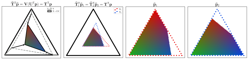
Figure 6: The intuition behind the theoretical results.

In this section, we discuss the intuition behind our theoretical results.

Given the only constraint of $\displaystyle{\bm{p}}({\widetilde{Y}}|X)={\widehat{{\bm{T}}}}^{\mathsf{T}}{\widehat{{\bm{p}}}}(Y|X)$, a feasible $\displaystyle{\widehat{{\bm{T}}}}$ can be any matrix that satisfies

$$\forall x\in{\mathcal{X}},{\bm{p}}({\widetilde{Y}}|X=x)\in{\mathrm{Conv}}({\widehat{{\bm{T}}}}),$$ (20)

and we can find $\displaystyle{\widehat{{\bm{p}}}}(Y|X)$ accordingly, if the function class is sufficiently large. This is the partial identifiability problem. On the other hand, in real-world problems, we hope that the clean class-posterior $\displaystyle{\bm{p}}(Y|X)$ is the “cleannest”, so at least

$$\nexists{\bm{S}}\in{\mathcal{T}},\textnormal{ s.t. }{\bm{p}}(Y|X)={\bm{S}}^{\mathsf{T}}{\bm{p}}^{\prime}(Y|X).$$ (21)

Otherwise, $\displaystyle{\bm{p}}({\widetilde{Y}}|X)=({\bm{S}}{\bm{T}})^{\mathsf{T}}{\bm{p}}^{\prime}(Y|X)$ also holds and $\displaystyle{\bm{p}}^{\prime}(Y|X)$ might be a better solution. Thus, we become less ambitious, ignore all intermediate possible solutions and only aim to find the “cleannest” one.

However, there could be multiple “cleannest” ones in this sense. An example is illustrated in Fig. 6. There could be $\displaystyle{\widehat{{\bm{T}}}}_{1}$, $\displaystyle{\widehat{{\bm{T}}}}_{2}$, and $\displaystyle{\widehat{{\bm{p}}}}_{1}(Y|X)$, $\displaystyle{\widehat{{\bm{p}}}}_{2}(Y|X)$, such that

$${\bm{p}}({\widetilde{Y}}|X)={\widehat{{\bm{T}}}}_{1}^{\mathsf{T}}{\widehat{{\bm{p}}}}_{1}(Y|X)={\widehat{{\bm{T}}}}_{2}^{\mathsf{T}}{\widehat{{\bm{p}}}}_{2}(Y|X),$$ (22)

and both $\displaystyle{\widehat{{\bm{p}}}}_{1}(Y|X)$ and $\displaystyle{\widehat{{\bm{p}}}}_{2}(Y|X)$ satisfy the condition above. In this sense, we still cannot distinguish $\displaystyle{\widehat{{\bm{p}}}}_{1}(Y|X)$ and $\displaystyle{\widehat{{\bm{p}}}}_{2}(Y|X)$. Either of them can be the true clean class-posterior.

To avoid such cases, in this work, we made the assumption that anchor points exist, i.e., there are instances for each class that we are absolutely sure which class they belong to. Such instances are considered prototypes of each class, and we believe that they exist in many real-world noisy datasets. In this way, we can guarantee the uniqueness of the “cleannest” clean class-posterior and the transition matrix, and consequently construct consistent estimators to find them, as explained in this paper.

If anchor points for all classes do not exist, the proposed algorithm may still work in practice but there is no theoretical guarantee yet. As mentioned in Section 5, Li et al. (2021) aims to relax the anchor point assumption. From the perspective of the geometric property of the transition matrix, it is possible to solve this problem in a weaker condition, which is, however, not the focus of this work.

Appendix E Experiments

In this section, we provide missing details of the experimental settings used in Section 6.

E.1 Benchmark Datasets

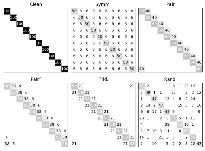
Figure 7: Synthetic transition matrices ($\displaystyle\times 100$) used in our experiments when $\displaystyle K=10$ (MNIST and CIFAR-10). The random noise matrix (Rand.) is an example while other matrices are fixed.

Data.

We used the MNIST, CIFAR-10, and CIFAR-100 datasets. The MNIST dataset contains $\displaystyle 28\times 28$ grayscale images in $\displaystyle 10$ classes. The size of the training set is $\displaystyle 60000$ and the size of the test set is $\displaystyle 10000$. The CIFAR-10 and CIFAR-100 datasets contain $\displaystyle 32\times 32$ colour images in $\displaystyle 10$ classes and in $\displaystyle 100$ classes, respectively. The size of the training set is $\displaystyle 50000$ and the size of the test set is $\displaystyle 10000$.

Data preprocessing.

For MNIST, We did not use any data augmentation. For CIFAR-10 and CIFAR-100, we used random crop and random horizontal flip. We added synthetic label noise into the training sets. The test sets were not modified. Overall, the transition matrices are plotted in Fig. 7. More specifically, we used:

1. (Clean) no additional synthetic noise, which serves as a baseline for the dataset and model.

2. (Symm.) symmetric noise with noise rate $\displaystyle 50\%$ (Patrini et al., 2017).

3. (Pair) pair flipping noise with noise rate $\displaystyle 40\%$ (Han et al., 2018b).

4. (Pair²) a product of two pair flipping noise matrices with noise rates $\displaystyle 30\%$ and $\displaystyle 20\%$. Because the multiplication of pair flipping noise matrices is commutative, it is guaranteed to have multiple ways of decomposition of the transition matrix, e.g., $\displaystyle{\bm{T}}_{\mathrm{pair}}(30\%){\bm{T}}_{\mathrm{pair}}(20\%)={\bm{T}}_{\mathrm{pair}}(20\%){\bm{T}}_{\mathrm{pair}}(30\%)$. The overall noise rate is $\displaystyle 44\%$.

5. (Trid.) tridiagonal noise (see also Han et al., 2018a), which corresponds to a spectral of classes where adjacent classes are easier to be mutually mislabeled, unlike the unidirectional pair flipping. It can be implemented by two consecutive pair flipping transformations in the opposite direction. We used $\displaystyle{\bm{T}}_{\mathrm{pair}}(30\%){\bm{T}}_{\mathrm{pair}}(30\%)^{\mathsf{T}}$ in the experiment. The overall noise rate is $\displaystyle 42\%$. Strictly, the matrix is not a tridiagonal matrix in the conventional sense because $\displaystyle{\bm{T}}_{1,K}$ and $\displaystyle{\bm{T}}_{K,1}$ are non-zero.

6. (Rand.) random noise constructed by sampling a Dirichlet distribution and mixing with the identity matrix to a specified noise rate. The higher the concentration parameter of the Dirichlet distribution is, the more uniform the off-diagonal elements of the transition matrix are. We used $\displaystyle 0.5$ in the experiment. Then, we mixed the sampled matrix with the identity matrix linearly to make the overall noise rate $\displaystyle 50\%$. The transition matrix is sampled for each trial.

Models.

For MNIST, we used a sequential convolutional neural network with the following structure: Conv2d(channel=$\displaystyle 32$) $\displaystyle\times 2$, Conv2d(channel=$\displaystyle 64$) $\displaystyle\times 2$, MaxPool2d(size=$\displaystyle 2$), Linear(dim=$\displaystyle 128$), Dropout(p=$\displaystyle 0.5$), Linear(dim=$\displaystyle 10$). The kernel size of convolutional layers is $\displaystyle 3$, and rectified linear unit (ReLU) is applied after the convolutional layers and linear layers except the last one. For both CIFAR-10 and CIFAR-100, we used a ResNet-18 model (He et al., 2016).

Optimization.

For MNIST, we used an Adam optimizer (Kingma & Ba, 2015) with batch size of $\displaystyle 512$ and learning rate of $\displaystyle 1\text{\times}{10}^{-3}$. The model was trained for $\displaystyle 2000$ iterations ($\displaystyle 17.07$ epochs) and the learning rate decayed exponentially to $\displaystyle 1\text{\times}{10}^{-4}$. For CIFAR-10 and CIFAR-100, we used a stochastic gradient descent (SGD) optimizer with batch size of $\displaystyle 512$, momentum of $\displaystyle 0.9$, and weight decay of $\displaystyle 1\text{\times}{10}^{-4}$. The learning rate increased from $\displaystyle 0$ to $\displaystyle 0.1$ linearly for $\displaystyle 400$ iterations and decreased to $\displaystyle 0$ linearly for $\displaystyle 3600$ iterations ($\displaystyle 4000$ iterations/$\displaystyle 40.96$ epochs in total).

For the gradient-based estimation, we used an Adam optimizer (Kingma & Ba, 2015). The learning rate increased from $\displaystyle 0$ to $\displaystyle 5\text{\times}{10}^{-3}$ linearly for $\displaystyle 400$ iterations and creased to $\displaystyle 0$ linearly for the rest iterations. This is helpful because at earlier stage, the model was not sufficiently trained yet and changing the transition matrix too much may destabilize the training of the model.

We tuned hyperparameters using grid search on a small experiment and fixed them in all experimental settings. For better reusability, we assumed that we are noise-agnostic and did not fine-tune hyperparameters for each noise type. If we have more prior knowledge about the noise, a better initialization may further improve the performance.

Infrastructure.

The experiments were conducted on NVIDIA Tesla P100 GPUs. We used a single GPU for MNIST and data-parallel on $\displaystyle 2$ GPUs for CIFAR-10 and CIFAR-100.

Results.

In addition to the accuracy and average total variation presented in Tables 1 and 2, we also provide the heat maps of the estimated transition matrices in Figs. 8, 9 and 10. Extremely small numbers are hided for better demonstration.

We can observe that our proposed method, especially the Dirichlet posterior update method, usually has better estimation of the transition matrix under various noise types. Dual-T (Yao et al., 2020) also performs well in some settings, which is also reflected in Table 2.

E.2 Clothing1M

Data.

Clothing1M (Xiao et al., 2015) is a real-world noisy label dataset. It contains $\displaystyle 47570$ clean training images, $\displaystyle 1\text{\times}{10}^{6}$ ($\displaystyle 1M$) noisy training images, $\displaystyle 14313$ clean validation images, and $\displaystyle 10526$ clean test images in $\displaystyle 14$ classes. We only used the noisy training data and clean test data.

Model and optimization.

We followed previous work (Patrini et al., 2017; Xia et al., 2019). We used a ResNet-50 model (He et al., 2016) pretrained on ImageNet and a SGD optimizer with momentum of $\displaystyle 0.9$, weight decay of $\displaystyle 1\text{\times}{10}^{-3}$, and batch size of $\displaystyle 32$. We trained the model on $\displaystyle 64$ GPUs for $\displaystyle 5000$ iterations ($\displaystyle 10.24$ epochs in total). The learning rate was $\displaystyle 1\text{\times}{10}^{-3}$ for the first half and $\displaystyle 1\text{\times}{10}^{-4}$ for the second half.

Other hyperparameters.

We initialized the concentration matrix with diagonal elements of $\displaystyle 1$ and off-diagonal elements of $\displaystyle 0$. We set $\displaystyle{\bm{\beta}}=(0.999,0.01)$ and $\displaystyle\gamma=0.1$.

Infrastructure.

We implemented data-parallel distributed training on $\displaystyle 64$ NVIDIA Tesla P100 GPUs by PyTorch (Paszke et al., 2019). The average runtime is about $\displaystyle 15$ (without SyncBatchNorm) to $\displaystyle 25$ (with SyncBatchNorm) minutes.

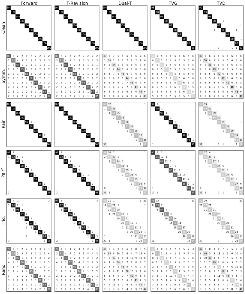
Figure 8: Estimated transition matrices ($\displaystyle\times 100$) on MNIST.

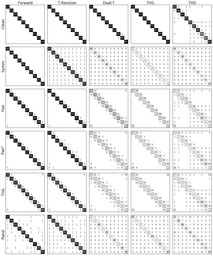
Figure 9: Estimated transition matrices ($\displaystyle\times 100$) on CIFAR10.

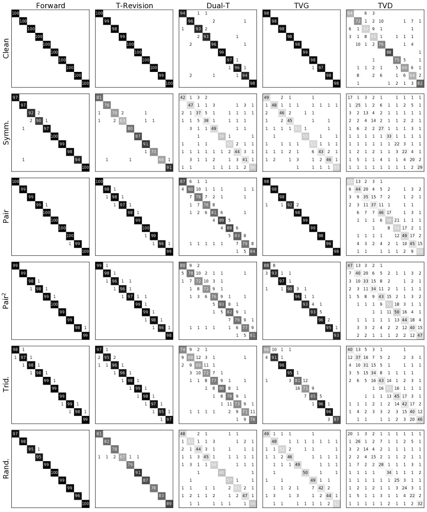
Figure 10: Estimated transition matrices ($\displaystyle\times 100$) on CIFAR100 (first $\displaystyle 10$ classes).

References

- Angluin & Laird (1988) Angluin, D. and Laird, P. Learning from noisy examples. Machine Learning, 2(4):343–370, 1988.
- Arpit et al. (2017) Arpit, D., Jastrzębski, S., Ballas, N., Krueger, D., Bengio, E., Kanwal, M. S., Maharaj, T., Fischer, A., Courville, A., Bengio, Y., et al. A closer look at memorization in deep networks. In Proceedings of the 34th International Conference on Machine Learning, 2017.
- Bartlett et al. (2006) Bartlett, P. L., Jordan, M. I., and McAuliffe, J. D. Convexity, classification, and risk bounds. Journal of the American Statistical Association, 101(473):138–156, 2006.
- Berthon et al. (2021) Berthon, A., Han, B., Niu, G., Liu, T., and Sugiyama, M. Confidence scores make instance-dependent label-noise learning possible. In Proceedings of the 38th International Conference on Machine Learning, 2021.
- Blanchard & Scott (2014) Blanchard, G. and Scott, C. Decontamination of mutually contaminated models. In Artificial Intelligence and Statistics, pp. 1–9, 2014.
- Charoenphakdee et al. (2019) Charoenphakdee, N., Lee, J., and Sugiyama, M. On symmetric losses for learning from corrupted labels. In Proceedings of the 36th International Conference on Machine Learning, pp. 961–970, 2019.
- Charoenphakdee et al. (2021) Charoenphakdee, N., Cui, Z., Zhang, Y., and Sugiyama, M. Classification with rejection based on cost-sensitive classification. In Proceedings of the 38th International Conference on Machine Learning, 2021.
- Chen et al. (2021) Chen, P., Ye, J., Chen, G., Zhao, J., and Heng, P.-A. Robustness of accuracy metric and its inspirations in learning with noisy labels. In Proceedings of the Thirty-Fifth AAAI Conference on Artificial Intelligence, 2021.
- Cheng et al. (2020) Cheng, J., Liu, T., Ramamohanarao, K., and Tao, D. Learning with bounded instance-and label-dependent label noise. In Proceedings of the 37th International Conference on Machine Learning, pp. 1789–1799, 2020.
- Cortes & Vapnik (1995) Cortes, C. and Vapnik, V. Support-vector networks. Machine learning, 20(3):273–297, 1995.
- Del Moral et al. (2003) Del Moral, P., Ledoux, M., and Miclo, L. On contraction properties of markov kernels. Probability theory and related fields, 126(3):395–420, 2003.
- Diaconis & Ylvisaker (1979) Diaconis, P. and Ylvisaker, D. Conjugate priors for exponential families. The Annals of statistics, pp. 269–281, 1979.
- du Plessis et al. (2014) du Plessis, M. C., Niu, G., and Sugiyama, M. Analysis of learning from positive and unlabeled data. In Advances in neural information processing systems, pp. 703–711, 2014.
- El-Yaniv & Wiener (2010) El-Yaniv, R. and Wiener, Y. On the foundations of noise-free selective classification. Journal of Machine Learning Research, 11(5), 2010.
- Feng et al. (2020) Feng, L., Shu, S., Lin, Z., Lv, F., Li, L., and An, B. Can cross entropy loss be robust to label noise? In Proceedings of the Twenty-Ninth International Joint Conference on Artificial Intelligence, pp. 2206–2212, 2020.
- Fergus et al. (2005) Fergus, R., Fei-Fei, L., Perona, P., and Zisserman, A. Learning object categories from Google’s image search. In Tenth IEEE International Conference on Computer Vision, volume 2, pp. 1816–1823, 2005.
- Ghosh et al. (2017) Ghosh, A., Kumar, H., and Sastry, P. Robust loss functions under label noise for deep neural networks. In Proceedings of the Thirty-First AAAI Conference on Artificial Intelligence, pp. 1919–1925, 2017.
- Goldberger & Ben-Reuven (2017) Goldberger, J. and Ben-Reuven, E. Training deep neural-networks using a noise adaptation layer. In International Conference on Learning Representations, 2017.
- Goodfellow et al. (2016) Goodfellow, I., Bengio, Y., Courville, A., and Bengio, Y. Deep learning. MIT press Cambridge, 2016.
- Guo et al. (2017) Guo, C., Pleiss, G., Sun, Y., and Weinberger, K. Q. On calibration of modern neural networks. In Proceedings of the 34th International Conference on Machine Learning, pp. 1321–1330, 2017.
- Han et al. (2018a) Han, B., Yao, J., Niu, G., Zhou, M., Tsang, I., Zhang, Y., and Sugiyama, M. Masking: A new perspective of noisy supervision. In Advances in Neural Information Processing Systems, pp. 5836–5846, 2018a.
- Han et al. (2018b) Han, B., Yao, Q., Yu, X., Niu, G., Xu, M., Hu, W., Tsang, I., and Sugiyama, M. Co-teaching: Robust training of deep neural networks with extremely noisy labels. In Advances in Neural Information Processing Systems, pp. 8527–8537, 2018b.
- He et al. (2016) He, K., Zhang, X., Ren, S., and Sun, J. Deep residual learning for image recognition. In Proceedings of the IEEE conference on computer vision and pattern recognition, pp. 770–778, 2016.
- Hein et al. (2019) Hein, M., Andriushchenko, M., and Bitterwolf, J. Why ReLU networks yield high-confidence predictions far away from the training data and how to mitigate the problem. In Proceedings of the IEEE Conference on Computer Vision and Pattern Recognition, pp. 41–50, 2019.
- Higgins et al. (2017) Higgins, I., Matthey, L., Pal, A., Burgess, C., Glorot, X., Botvinick, M., Mohamed, S., and Lerchner, A. beta-VAE: Learning basic visual concepts with a constrained variational framework. In International Conference on Learning Representations, 2017.
- Ishida et al. (2017) Ishida, T., Niu, G., Hu, W., and Sugiyama, M. Learning from complementary labels. In Advances in neural information processing systems, pp. 5639–5649, 2017.
- Jiang et al. (2018) Jiang, L., Zhou, Z., Leung, T., Li, L.-J., and Fei-Fei, L. MentorNet: Learning data-driven curriculum for very deep neural networks on corrupted labels. In Proceedings of the 35th International Conference on Machine Learning, pp. 2304–2313, 2018.
- Jiang et al. (2020) Jiang, L., Huang, D., Liu, M., and Yang, W. Beyond synthetic noise: Deep learning on controlled noisy labels. In Proceedings of the 37th International Conference on Machine Learning, pp. 4804–4815, 2020.
- Kingma & Ba (2015) Kingma, D. P. and Ba, J. Adam: A method for stochastic optimization. In 3rd International Conference on Learning Representations, 2015.
- Kloft et al. (2009) Kloft, M., Brefeld, U., Sonnenburg, S., Laskov, P., Müller, K., and Zien, A. Efficient and accurate -norm multiple kernel learning. In Advances in Neural Information Processing Systems, pp. 997–1005, 2009.
- Krizhevsky (2009) Krizhevsky, A. Learning multiple layers of features from tiny images, 2009.
- Kuhn et al. (1951) Kuhn, H., Tucker, A., et al. Nonlinear programming. In Proceedings of the Second Berkeley Symposium on Mathematical Statistics and Probability. The Regents of the University of California, 1951.
- Kull et al. (2019) Kull, M., Nieto, M. P., Kängsepp, M., Silva Filho, T., Song, H., and Flach, P. Beyond temperature scaling: Obtaining well-calibrated multi-class probabilities with dirichlet calibration. In Advances in neural information processing systems, pp. 12316–12326, 2019.
- LeCun et al. (1998) LeCun, Y., Bottou, L., Bengio, Y., and Haffner, P. Gradient-based learning applied to document recognition, 1998.
- Li et al. (2019) Li, J., Wong, Y., Zhao, Q., and Kankanhalli, M. S. Learning to learn from noisy labeled data. In Proceedings of the IEEE/CVF Conference on Computer Vision and Pattern Recognition, pp. 5051–5059, 2019.
- Li et al. (2020) Li, J., Socher, R., and Hoi, S. C. DivideMix: Learning with noisy labels as semi-supervised learning. In International Conference on Learning Representations, 2020.
- Li et al. (2021) Li, X., Liu, T., Han, B., Niu, G., and Sugiyama, M. Provably end-to-end label-noise learning without anchor point. In Proceedings of the 38th International Conference on Machine Learning, 2021.
- Liu & Tao (2015) Liu, T. and Tao, D. Classification with noisy labels by importance reweighting. IEEE Transactions on pattern analysis and machine intelligence, 38(3):447–461, 2015.
- Liu & Guo (2020) Liu, Y. and Guo, H. Peer loss functions: Learning from noisy labels without knowing noise rates. In Proceedings of the 37th International Conference on Machine Learning, pp. 6226–6236, 2020.
- Long & Servedio (2010) Long, P. M. and Servedio, R. A. Random classification noise defeats all convex potential boosters. Machine learning, 78(3):287–304, 2010.
- Lu et al. (2019) Lu, N., Niu, G., Menon, A. K., and Sugiyama, M. On the minimal supervision for training any binary classifier from only unlabeled data. In International Conference on Learning Representations, 2019.
- Lyu & Tsang (2020) Lyu, Y. and Tsang, I. W. Curriculum loss: Robust learning and generalization against label corruption. In International Conference on Learning Representations, 2020.
- Ma et al. (2020) Ma, X., Huang, H., Wang, Y., Romano, S., Erfani, S., and Bailey, J. Normalized loss functions for deep learning with noisy labels. In Proceedings of the 37th International Conference on Machine Learning, pp. 6543–6553, 2020.
- Malach & Shalev-Shwartz (2017) Malach, E. and Shalev-Shwartz, S. Decoupling “when to update” from “how to update”. In Advances in Neural Information Processing Systems, pp. 960–970, 2017.
- Menon et al. (2015) Menon, A., Van Rooyen, B., Ong, C. S., and Williamson, B. Learning from corrupted binary labels via class-probability estimation. In Proceedings of the 32nd International Conference on Machine Learning, pp. 125–134, 2015.
- Menon et al. (2018) Menon, A. K., Van Rooyen, B., and Natarajan, N. Learning from binary labels with instance-dependent noise. Machine Learning, 107(8-10):1561–1595, 2018.
- Mirzasoleiman et al. (2020) Mirzasoleiman, B., Cao, K., and Leskovec, J. Coresets for robust training of deep neural networks against noisy labels. In Advances in Neural Information Processing Systems, 2020.
- Mozannar & Sontag (2020) Mozannar, H. and Sontag, D. Consistent estimators for learning to defer to an expert. In International Conference on Machine Learning, pp. 7076–7087, 2020.
- Natarajan et al. (2013) Natarajan, N., Dhillon, I. S., Ravikumar, P. K., and Tewari, A. Learning with noisy labels. In Advances in neural information processing systems, pp. 1196–1204, 2013.
- Nguyen et al. (2020) Nguyen, D. T., Mummadi, C. K., Ngo, T. P. N., Nguyen, T. H. P., Beggel, L., and Brox, T. SELF: Learning to filter noisy labels with self-ensembling. In International Conference on Learning Representations, 2020.
- Paszke et al. (2019) Paszke, A., Gross, S., Massa, F., Lerer, A., Bradbury, J., Chanan, G., Killeen, T., Lin, Z., Gimelshein, N., Antiga, L., et al. PyTorch: An imperative style, high-performance deep learning library. In Advances in neural information processing systems, pp. 8026–8037, 2019.
- Patrini et al. (2017) Patrini, G., Rozza, A., Krishna Menon, A., Nock, R., and Qu, L. Making deep neural networks robust to label noise: A loss correction approach. In Proceedings of the IEEE Conference on Computer Vision and Pattern Recognition, pp. 1944–1952, 2017.
- Rahimi et al. (2020) Rahimi, A., Shaban, A., Cheng, C.-A., Hartley, R., and Boots, B. Intra order-preserving functions for calibration of multi-class neural networks. In Advances in Neural Information Processing Systems, 2020.
- Ramaswamy et al. (2016) Ramaswamy, H., Scott, C., and Tewari, A. Mixture proportion estimation via kernel embeddings of distributions. In Proceedings of The 33rd International Conference on Machine Learning, pp. 2052–2060, 2016.
- Scott (2015) Scott, C. A rate of convergence for mixture proportion estimation, with application to learning from noisy labels. In Proceedings of the Eighteenth International Conference on Artificial Intelligence and Statistics, pp. 838–846, 2015.
- Scott et al. (2013) Scott, C., Blanchard, G., and Handy, G. Classification with asymmetric label noise: Consistency and maximal denoising. In Proceedings of the 26th Annual Conference on Learning Theory, pp. 489–511, 2013.
- Shu et al. (2019) Shu, J., Xie, Q., Yi, L., Zhao, Q., Zhou, S., Xu, Z., and Meng, D. Meta-Weight-Net: Learning an explicit mapping for sample weighting. In Advances in Neural Information Processing Systems, 2019.
- Sutskever et al. (2013) Sutskever, I., Martens, J., Dahl, G., and Hinton, G. On the importance of initialization and momentum in deep learning. In International conference on machine learning, pp. 1139–1147, 2013.
- Tewari & Bartlett (2007) Tewari, A. and Bartlett, P. L. On the consistency of multiclass classification methods. Journal of Machine Learning Research, 8(May):1007–1025, 2007.
- Thulasidasan et al. (2019) Thulasidasan, S., Bhattacharya, T., Bilmes, J., Chennupati, G., and Mohd-Yusof, J. Combating label noise in deep learning using abstention. In International Conference on Machine Learning, pp. 6234–6243, 2019.
- Van Rooyen et al. (2015) Van Rooyen, B., Menon, A., and Williamson, R. C. Learning with symmetric label noise: The importance of being unhinged. In Advances in Neural Information Processing Systems, pp. 10–18, 2015.
- Wang et al. (2018) Wang, Y., Liu, W., Ma, X., Bailey, J., Zha, H., Song, L., and Xia, S.-T. Iterative learning with open-set noisy labels. In Proceedings of the IEEE Conference on Computer Vision and Pattern Recognition, pp. 8688–8696, 2018.
- Wang et al. (2019) Wang, Y., Ma, X., Chen, Z., Luo, Y., Yi, J., and Bailey, J. Symmetric cross entropy for robust learning with noisy labels. In Proceedings of the IEEE International Conference on Computer Vision, pp. 322–330, 2019.
- Wei et al. (2020) Wei, H., Feng, L., Chen, X., and An, B. Combating noisy labels by agreement: A joint training method with co-regularization. In Proceedings of the IEEE/CVF Conference on Computer Vision and Pattern Recognition, pp. 13726–13735, 2020.
- Wu et al. (2020) Wu, P., Zheng, S., Goswami, M., Metaxas, D., and Chen, C. A topological filter for learning with label noise. In Advances in Neural Information Processing Systems, 2020.
- Xia et al. (2019) Xia, X., Liu, T., Wang, N., Han, B., Gong, C., Niu, G., and Sugiyama, M. Are anchor points really indispensable in label-noise learning? In Advances in Neural Information Processing Systems, pp. 6838–6849, 2019.
- Xia et al. (2020) Xia, X., Liu, T., Han, B., Wang, N., Gong, M., Liu, H., Niu, G., Tao, D., and Sugiyama, M. Part-dependent label noise: Towards instance-dependent label noise. In Advances in Neural Information Processing Systems, 2020.
- Xiao et al. (2015) Xiao, T., Xia, T., Yang, Y., Huang, C., and Wang, X. Learning from massive noisy labeled data for image classification. In Proceedings of the IEEE conference on computer vision and pattern recognition, pp. 2691–2699, 2015.
- Yao et al. (2020) Yao, Y., Liu, T., Han, B., Gong, M., Deng, J., Niu, G., and Sugiyama, M. Dual T: Reducing estimation error for transition matrix in label-noise learning. In Advances in Neural Information Processing Systems, 2020.
- Yu et al. (2018) Yu, X., Liu, T., Gong, M., and Tao, D. Learning with biased complementary labels. In Proceedings of the European Conference on Computer Vision (ECCV), pp. 68–83, 2018.
- Yu et al. (2019) Yu, X., Han, B., Yao, J., Niu, G., Tsang, I., and Sugiyama, M. How does disagreement help generalization against label corruption? In Proceedings of the 36th International Conference on Machine Learning, pp. 7164–7173, 2019.
- Zhang et al. (2017) Zhang, C., Bengio, S., Hardt, M., Recht, B., and Vinyals, O. Understanding deep learning requires rethinking generalization. In International Conference on Learning Representations, 2017.
- Zhang & Sabuncu (2018) Zhang, Z. and Sabuncu, M. Generalized cross entropy loss for training deep neural networks with noisy labels. In Advances in neural information processing systems, pp. 8778–8788, 2018.